
Submitted:
17 April 2025
Posted:
19 April 2025
You are already at the latest version
Abstract
This paper offers educational insight into the Dirac equation, examining its historical context and contrasting it with the earlier Schrödinger and Klein-Gordon (KG) equations. The comparison highlights their Lorentz transformation symmetry and potential probabilistic interpretations. We explicitly solve the free-particle dynamics in Dirac's model, revealing the emergence of negative-energy solutions. This discussion examines the Dirac Sea Hypothesis and explores the solutions' inherent helicity. Additionally, we demonstrate how the Dirac equation accounts for spin and derive the Pauli equation in the non-relativistic limit. The Foldy-Wouthuysen transformation reveals how the equation incorporates spin-orbit interaction and other relativistic effects, ultimately leading to the fine structure of hydrogen. A section on relativistic covariant notation is included to emphasize the invariance of the Dirac equation, along with more refined formulations of both the KG and Dirac equations. Designed for undergraduate students interested in the Dirac equation, this resource provides a historical perspective without being purely theoretical. Our approach underscores the significance of a pedagogical method that combines historical and comparative elements to profoundly understand the role of the Dirac equation in modern physics.
Keywords:
Relativisitc equation
; spin
; positron
1. Introduction
The Dirac equation, conceived by Paul Dirac in 1928 [1,2], is one of the cornerstones of contemporary physics, merging the principles of special relativity and quantum mechanics. This equation not only predicts antiparticles but also contains the Pauli equation in the non-relativistic limit, consequently incorporating the concept of spin. Revered as a milestone in scientific history [3], it is also distinguished by its beauty, as highlighted by Wilczek [4]: “Of all the equations of physics, perhaps the most magical is the Dirac equation”. Moreover, the applications of Dirac theory span various domains, including Quantum Field Theory [5,6], Material Science [7,8], and Cosmology [9,10].
Beyond its mathematical and physical significance, the equation garners attention outside academia, prominently featured in scientific dissemination materials [11,12]. This widespread coverage underscores its emblematic importance within modern physics. However, despite its stature, Dirac’s model often remains unexplored in undergraduate studies. Hence, our proposal aims to bridge this gap by presenting a didactic introduction to the equation, not claiming to make an original contribution to Relativistic Quantum Mechanics or to the History of Physics while doing so.
Similar efforts have been undertaken [3,13,14], and our aim is to complement them by emphasizing the historical context coupled with the comparison between the wave equations. Keeping in mind the didactic purpose of this work, we have included information beyond the wave equations, such as a historical preamble and insights and anecdotes from Dirac throughout the article. While this may seem tangential, we believe these additional details, besides arousing the reader’s curiosity, may provide a deeper understanding of the nuances of the man who formulated the equation.
This work is intended for undergraduate students who are fascinated by the subject, but are not content with a purely conceptual approach. Instead, we utilize mathematical tools commonly taught in the early years of graduation, ensuring that the article remains accessible without posing significant challenges. We instructively present key concepts of quantum mechanics to the less familiar reader, aiming to do so smoothly and contextually to avoid boring the more experienced reader. For instances requiring more formal computation, we strive to clarify the steps explicitly, accompanied by further recommended readings to aid comprehension. Consciously, we have chosen not to use the Dirac-Braket notation, as it is typically not employed in the initial encounters with quantum mechanics. Exceptions are made in the Appendix A, where the notation significantly facilitates the discussion regarding the dimension of the Dirac matrices, and in SubSection 6.2, where detailed calculations would be quite extensive.
Furthermore, we seek to fill a gap in references that address the incongruity between the Schrödinger equation and the relativity [3,15,16]. Surprisingly, even Relativistic Quantum Mechanics books [17,18] may lack this discussion, usually starting the detailed analysis from the Klein-Gordon (KG) equation onward. To tackle this issue, we choose to demonstrate the equation’s non-invariance using a simple one-dimensional Lorentz transformation, a key principle from Relativity Theory, explained as in introductory Modern Physics classes [19]. We carry out this invariance test using the same methodology as the KG equation so that the contrast between the models is favored. This direct comparison between the wave equations is intensified so that the reader can perceive the distinctive characteristics of each equation. Reference [20] is an inspiration in this regard, as it draws an analogous comparison between the models but is restricted to the more complex case of atoms resembling hydrogen.
Moreover, we make use of covariant relativistic notation to highlight, in a non-rigorous fashion, the invariance of the Dirac equation and present more insightful versions of both the KG and Dirac equations. We presume that the reader, interested in the Dirac equation, has encountered its more refined form expressed through this notation. Consequently, we contend that learning the relativistic covariant notation is beneficial and fosters a deeper understanding of the equation.
2. Historical Preamble
The development of the Dirac equation is intricately connected to the progression of quantum mechanics and Dirac’s professional journey. This section explores the historical context of quantum theory leading to the introduction of wave mechanics, as we believe that understanding the scope of quantum physics prior to introducing the initial wave equation is vital to understanding the significance of the Schrödinger equation. Recommended supplementary readings include [21], which highlights Born’s influence during this era and elaborates further on matrix mechanics, and [22], which concentrates on Dirac’s role before the formulation of his equation.
On 21 September 1925, Werner Heisenberg published an exploratory article titled Quantum-theoretical re-interpretation of kinematic and mechanical relations [23] in response to discrepancies between experimental observations and theoretical predictions regarding the spectral lines of the hydrogen emission spectrum [24,208]. In this work, a significant transition was signaled, moving away from the Old Quantum Mechanics period. This era included major breakthroughs in quantum physics between 1900 and 1925, including the de Broglie hypothesis, the Pauli exclusion principle, and the Bohr-Sommerfeld atom model [25,28]. Despite successes, the Old Quantum Mechanics exhibited methodological gaps, relying on an amalgamation of hypotheses, principles, and theorems [24]. While Bohr endeavored to reconcile spectral line discrepancies through his correspondence principle, Heisenberg diverged from such approaches and classical methods, choosing instead to ground his theory on measurable observables. Fundamentally, he departed from non observable quantities within the quantum scope. For example, instead of using the position of an electron traversing an orbit, one should utilize the probability amplitude of the particle undergoing a transition from state n to state m [21]. Based on this reasoning, he formulates his well-known multiplication rule, by which two observables, such as and , are multiplied to form a new observable , which represents a combination of the original observables
A broad discussion of the mathematics of this topic is found in [24]. However, computing the product (1) in reverse order, that is, and , generally produces a different combination, so that . Remarkably, this differs from the classical theory, where the product of two quantities (c-numbers), a and b is independent of the order, i.e., .
In Heisenberg’s algebraic framework, Born identified matrix properties, a subject rarely utilized in physics until then [24,218]. Consequently, one would infer that Heisenberg’s observables, representing physical quantities in quantum mechanics, took the form of matrices. Born, along with Jordan, devised what would become known as matrix mechanics in their 1925 publication, "On Quantum Mechanics" [26], received merely six days after the publication of Heisenberg’s article in the same scientific journal Zeitschrift für Physik. By applying the Heisenberg rule, they successfully derived the canonical commutation relation in matrix form [21]
where h is Planck’s constant, is the unity matrix in dimensions and and are matrices or observables. This asserts that it is impossible for states to measure both a definite position and momentum simultaneously, a realization that is one of the foundations of quantum mechanics. In November 1926, a follow-up to the initial paper [27], this time co-authored by Heisenberg, was published. This publication further established the principles of matrix mechanics with greater thoroughness and detail, and Born famously called it the "three-man paper".
Dirac, in turn, noticed an initially perplexing relation in Heisenberg’s article that, weeks later, would lead to his first publication in quantum mechanics: the non-commutation between certain pairs of physical quantities [16]. This relationship underwent a period of contemplation before Dirac, on a Sunday in October 1925, linked it to the Poisson brackets [28,28], which are crucial components of Hamiltonian formalism in Classical Mechanics. In December 1925, The Fundamental Equations of Quantum Mechanics [29] is published, wherein, without using Heisenberg products or matrix properties, it was established the commutation relation
where x and p are what would soon be called operators, or, in Dirac terms, "q-numbers", and J.s is the reduced Planck’s constant. Here
is the commutator between x and p, which, when associated with Poisson brackets, illustrates a connection between quantum theory and the Hamiltonian formalism that Dirac aimed to achieve. Dirac’s aspiration originated from his conviction that classical equations retained their validity, although they needed alterations in their inherent mathematical properties . The process of quantizing classical theories, just as Dirac did with Poisson brackets, is called canonical quantization.
Despite the independent deduction of this relationship, Dirac’s work was well received. He was only 23 years old and still a student at Cambridge, so Born would remark: “The name Dirac was completely unknown to me. The author seemed to be a young man, but everything was perfect in his way and admirable” [30]. Moreover, by offering a more coherent theoretical framework, matrix theory was notably strong as Pauli employed matrix mechanics to derive the Balmer formula for hydrogen atom spectra [31] – albeit with the aid of supplementary assumptions [32]. However, the theory of Heisenberg, Born and Jordan was not immune to criticism: there were problems with respect to the physical interpretation of the theory, as well as a difficulty in defining a stationary state [32]. Furthermore, there was a lack of familiarity with the mathematics involved and the concepts adopted. For instance, Fermi only attained a comprehensive understanding of quantum theory through Schrödinger’s wave mechanics [24]. The timeline in Figure 1, presented out of scale, illustrates some of the most crucial events within the scope of this article.
3. Schrödinger Equation
In the first semester of 1926, while Dirac was pursuing his Ph.D., Erwin Schrödinger published four works on wave mechanics [33,34,35,36], all titled Quantization as an eigenvalue problem. Schrödinger’s initial goal was to derive an equation for de Broglie’s matter waves and, to this end, he used Hamilton’s optical-mechanics analogy [24,37]. He proposed that classical mechanics represents a specific instance within the broader scope of mechanics, encompassing microscopic scenarios, a parallel to geometric optics within the wider domain of optics. Consequently, classical equations were as ineffective for quantum problems as geometric optics for wavelike problems. Therefore, it was necessary to establish wave mechanics akin to physical optics, with the wave equation replacing classical equations of motion. In hindsight, this approach reflects Dirac’s convictions about the connections of quantum mechanics with the relations in classical physics, as discussed in the preceding section.
The derivation of the Schrödinger equation presented here emphasizes some important aspects regarding the quantization framework, which will be revisited throughout the reading. We commence with the classical relationship between energy E and momentum,
where m is the mass of the classical particle and the potential energy, depending on both the position vector and time t. Schrödinger proposed the following substitutions [38]
The relations above are a clear example of canonical quantization. Replacements (6) and (7) symbolize an important step in quantum mechanics: the transition of quantities to operators, which are specific kinds of linear transformation present in linear algebra. Replacing the aforementioned operators in (5) we obtain
where is the Laplacian differential operator
In Eq. (8), the operators appear on both sides, acting on the states to acquire physical significance. For now, the state undergoing the action of operators is the function . By applying both sides of (8) to the state , we obtain
a linear partial differential equation, which is referred to as time-dependent Schrödinger equation. The function is precisely the solution of this differential equation, a complex valued function of the position and time associated with the matter wave.
In quantum mechanics, the operator linked to energy is termed Hamiltonian, denoted as H from now onward, while E will be used to represent an energy quantity – occasionally replaced by its corresponding operator (6). Besides being proportional to the time derivative, the Hamiltonian can be formulated in terms of other operators, depending on the specific model under consideration. For Eq. (10), it can be represented as
Thus, the Hamiltonian is defined in such a way that it enables us to express Eq. (10) as
which is applicable, as we will see later, to other models beyond the Schrödinger one, and for this reason, it is called generalized Schrödinger equation.
The relationship between eigenvalues and quantum-mechanical operators is distinctive, enabling the derivation of concrete physical outcomes. When an operator is applied to a specific quantum state, defined by a given eigenfunction, the result is the same state multiplied by a scalar. The eigenvalue approach of Schrödinger consists precisely in applying this aforementioned relation, using the Hamiltonian extracted from his equation as an operator and making it act on the state , that is, an eigenfunction of H. The eigenvalues arise as solutions to the equation
By employing this method, Schrödinger notably succeeded in deriving the energy levels that correspond to Bohr’s non-relativistic model for the Hydrogen atom. Schödinger [36] had an electrodynamic interpretation of his wave equation, assuming that the square modulus of was a function of the charge distribution. However, in June 1926, Born introduced his probabilistic interpretation [16,39,260], considering the square modulus of as a probability density
where is always positive. Later in this section, when we discuss the free particle, we will exemplify this interpretation.
By manipulating (10), its conjugate, and (14), we can derive the equation of continuity
where is the probability current, defined as
where we leave the position and time variables of implicit.
Within the frameworks of Electromagnetism and Fluid Dynamics, Eq. (15) represents the principle of charge conservation and the conservation of fluid mass, respectively. Concerning the Schrödinger equation, it signifies conservation of probability. It is natural to wonder how wave mechanics fits in with matrix mechanics. In his third article [35], Schrödinger established that wave mechanics implies some concepts from matrix mechanics. John von Neumann, only in 1929, formally demonstrated the equivalence between matrix mechanics and wave mechanics, based on a functional analysis theorem [24,273].
An essential solution of the Schrödinger equation pertinent to this study involves a free particle. In this scenario, the differential equation allows for a solution resembling a plane wave, akin to the solution found in Maxwell’s equations within a vacuum
If we consider the one-dimensional and time-independent case, with the associated particle confined in a box of length L, the Schrödinger equation admits sinusoidal solutions , as illustrated in Figure 2, with positions A, B, and C taken as examples. According to the magnitude of the squared modulus (112), it can be observed that the decreasing order of probability for these positions is A, C, and B. The reader more familiar with quantum mechanics recognizes that, due to the probabilistic interpretation, the integration of over the length of the box (from to ) yields unity. This procedure, commonly found in textbook problems, usually seeks to identify the normalization constant of the specified wave function. The energy eigenvalues for this case are obtained through the equation
from where we extract what seems to be a prerequisite, but later we will discover that it is not: positive definite energy eigenvalues.
The scientific community received the Schrödinger equation with enthusiasm, and prominent personalities such as Fritz London, Charles Darwin, and Enrico Fermi were among those who welcomed it. Its emergence was almost reassuring in the context of the departure from classical methods advocated by the newer generation of physicists [4,110]. At the Munich Conference in the summer of 1926, most participants aligned themselves with wave mechanics to the detriment of matrix mechanics [32].
On the other hand, Dirac had an initial aversion to Schrödinger’s equation [16,287], since he had already developed his own methodology to address quantum problems involving the aforementioned q-numbers. However, he gradually accepted the Schrödinger equation as a complement to his theory and applied wave mechanics to problems with many particles [40]; in the same paper, he introduced his transformation theory. One characteristic of this theory is that it generalizes Born’s probabilistic interpretation of the Schrödinger equation [41].
The merits of the Schrödinger wave equation are vast and are widely covered in the literature [42,43,44,45]. Planck would say that “plays the same role in modern physics as the equations established by Newton, Lagrange, and Hamilton in classical mechanics” [46,30]. However, for the purposes of this article, we will address its limitations.
Feynman asserted that the Schrödinger equation is "capable of explaining all atomic phenomena, except those involving magnetism and relativity" [44,439]. This prompts the question: why does the equation not conform to relativity? A physical model is considered compatible with relativity when it remains invariant under Lorentz transformation, a linear transformation that converts coordinates from one reference frame to another, moving at a constant speed relative to the first, replacing the Galilean transformation of Newtonian physics. This transformation serves as a tool to assess whether a given equation aligns with the principles of relativity. A notable example of invariance is found in the solution of Maxwell’s equations for a vacuum (17), where the orders of spatial (Laplacian) and temporal derivatives are equal. On the other hand, equation (10), due to the different orders of derivatives, intuitively suggests a lack of “equality” between space and time as proposed by Einstein’s theory; this is the brief explanation provided by the majority of textbooks [3,15,16].
We will demonstrate that intuition is correct through a somewhat informal one-dimensional deduction. Therefore, we consider that in a reference frame , our wave function is , and in a reference frame moving with constant speed v relative to , the wave function is . Figure 3 illustrates the reference frames, and the Lorentz transformation, in this case, tells us how the position (x and ) and the time (t and ) in the two reference frames are related.
The structure of the equation must remain unchanged during a coordinate transformation to maintain the covariance of the physical laws governed by it. The solutions in different reference frames assume distinct functional forms which justify our writing of . We start with the Schrödinger equation for the wave function in the reference frame O in the form
and perform the transformation from to searching for the equation that satisfies for the potential . The one-dimensional Lorentz transformation in this case is
where is the Lorentz factor
Analyzing the Schrödinger equation (10), it is clear that to find the equation satisfied by , we must first write and in terms of and . Applying the chain rule, we have
The second derivative as a function of x is, again with the chain rule
Repeating the same procedure as above for the first order derivative of t, we obtain
We will not consider the second derivative of time in Schrödinger equation for now, but we will deduce the expression as it will be useful throughout the next section
One can use Eqs. (24) and (26) into the electromagnetic wave equation, Eq. (17), considering the one-dimensional case, and see that it is truly invariant. On the other hand, doing the same in Eq. (10) we have
Thus, comparing with Eq. (19), it becomes evident that the Schrödinger equation is not invariant under Lorentz transformation. Therefore, it is not proper when applied to relativistic particles.
Someone might wonder, out of interest, how the equation remains valid in a non-relativistic parallel scenario: Is it invariant under Galilean transformation? In a one-dimensional Galilean transformation, the relation between position and time in the two reference frames is given by
so that the first-order spatial derivative is
and the second order is
Furthermore, the time derivative is
Inserting Eqs. (31) and (32) into Eq. (10), we obtain
which can be written as
The second term on the right-hand side of Eq. (34) indicates that the Schrödinger equation is not invariant under the Galilean transformation. It is necessary to add a phase so that the wave function remains consistent [48], and the probabilities do not change [49].
Initially, Schrödinger himself attempted to derive a valid relativistic equation, but was unsuccessful in calculating the energy eigenvalues [24,258] according to the experimentally successful Sommerfeld energy levels, derived from the quantization of the relativistic Bohr atom. The Sommerfeld expression [50] for the energy eigenvalues of the hydrogen atom is
where c means the speed of light in vacuum, is the fine structure constant, n corresponds to the principal quantum number and k represents the azimuthal quantum number. Sommerfeld’s relativistic correction is associated with the splitting of hydrogen spectral lines, known as the fine structure of hydrogen.
In Eq. (35), Schrödinger obtained and instead of and k, respectively [3]. However, it is known that this error is due to the non incorporation of electron spin into the equation [24,258]. Schrödinger eventually informed Dirac that he had developed a relativistic wave equation, but it was unable to reproduce the Sommerfeld formula. In particular, Dirac displayed a noteworthy perspective, stating that the colleague should have maintained confidence in his “beautiful relativistic theory”, even if it was inconsistent with accurate experimental data [28]. A more in-depth discussion of this aspect of Schrödinger’s theory can be found in [51].
4. Klein-Gordon Equation
During 1926, a possible relativistic wave equation was derived by at least seven authors: Klein [52], Schrödinger [36], Fock [53], Donder, Dungen [54], Kudar [55] and Gordon [56]. Priority in the nomenclature is given to Oscar Klein, who proposed the equation in April 1926, while Fock provided a more intricate exploration of relativistic wave mechanics [3]. We will follow the more direct derivation, starting from the relativistic relation between energy E and linear momentum , expressed as
where the potential energy is taken as zero and m refers to the rest mass. We can replace both E and quantities in Eq. (36) by operators the operator in Eqs. (6) and (7), so that we obtain
that we can apply the both sides to to arrive at the equation
which can be written as
Moreover, employing the d’Alembertian operator and the constant , equation (39) can be put in the form
which is called scalar wave equation or Klein-Gordon equation (KG from now on). There is another way to write it, using relativistic covariant notation and natural units, which we will show later.
The KG equation aims to adhere to the principles of relativity, prompting an initial assessment of its conformity from this perspective. Notably, one aspect that immediately draws attention is the similarity between equation (39) and the electric field wave equation (17) – in fact, one can obtain the former from the latter, as shown by [57,58]. Furthermore, we analyze the orders of the space and temporal derivatives, and we see that they are equal: this leads to the intuition that the KG equation is invariant under a Lorentz transformation. A parallel analysis, akin to our examination of the Schrödinger equation, is now applied to the one-dimensional form of the KG equation, i.e.,
in which we incorporate Eqs. (24) and (25), we arrive at
so that we rewrite it as
where we can employ the definition of the Lorentz factor (22), so that
demonstrating that the KG equation remains invariant under Lorentz transformation.
Another crucial aspect of the KG equation is investigating its applicability in physical systems, particularly considering the range of problems that can be addressed with the Schrödinger equation. Therefore, applying the KG equation to a simple system and testing its validity is only fair. For instance, as an elementary problem, let us analyze the energy eigenvalues of a free particle. Taking Eq. (39) and simplifying it, we have
which is expected to have plane-wave solutions with a time dependency of the type and a spatial dependence of the type , so that
where N is a normalization constant and · symbolizes the scalar product. Equation (46) is a solution of Eq. (45) if
which includes both positive and negative energy eigenvalues. This may seem counterintuitive, but it is now understood that negative energy solutions are valid. However, when the concept of antiparticles was unknown, this posed an obstacle to accepting the KG equation. In the next section, we will discuss this intriguing aspect, which arises as a solution to the free particle.
Additionally, an important aspect to study is how the probability density . It is desirable that be conserved and positive definite in this model, as it happens in the Schrödinger equation. In this manner, we obtain the following equation for the probability density
where we note that, although it is a preserved quantity, is not positive definite, unlike Eq. (14). This posed an immediate challenge as it complicated the probabilistic interpretation of the wave function. Nevertheless, we now know that the correct interpretation is that is a probability charge density [42,482].
Initially, the KG equation was considered the correct relativistic generalization of wave mechanics: It possessed the inherent elegance of symmetry and, thus, was invariant under the Lorentz transformation. Schrödinger himself would use it in subsequent approaches to the Compton effect, a phenomenon that encompasses relativistic effects. However, despite its mathematical appeal, its applications were limited compared to the Schrödinger equation, especially considering the lack of widely accepted explanations for negative energies. This meant that, even though some physicists believed that the problem of relativistic generalization was already solved with the KG equation, the quest for a more suitable wave equation persisted. However, it should be noted that in quantum field theory, the KG equation finds validity for pions, which are spinless particles [6]. Additionally, it is instructive to note that in the non-relativistic limit, the KG equation reduces to the Schrödinger equation [59].
5. Pauli Equation
An important event in the search for a relativistic wave equation was the discovery of spin, initially believed to be intrinsically relativistic. The first indication of spin’s existence arose from the Stern-Gerlach (SG) experiment [60], where an atomic beam of silver was subjected to an inhomogeneous magnetic field. Silver’s 47th electron’s magnetic moment approximates the atom’s magnetic moment because of its specific structure. If the electron behaved classically, its magnetic moment would exhibit a continuous range of values, resulting in a Gaussian pattern after passing through the magnetic field. However, in the SG experiment, deviations were observed for all atoms, with detection occurring in two preferential regions, as illustrated in Figure 4. This suggested that the magnetic moment of the electron had only two directions, a phenomenon which Sommerfeld interpreted as evidence of space quantization [24,131].
Pauli began the study of this paradigm by examining the hyperfine structure of the hydrogen atom, proposing that the nucleus possesses an angular momentum that does not simply “disappear” [61]. In November 1925, Dutch physicists Uhlenbeck and Goudsmit expanded this notion by offering a more thorough explanation of this novel quantum property [62]. They introduced a new quantum number associated with an extra degree of freedom connected to the electron’s magnetic moment, called spin. This quantum number had two observable states in the SG experiment: spin up and spin down. The recognition of spin highlighted its essential role in quantum theory.
First, let us discuss how the Schrödinger equation deals with electromagnetic interactions by writing it as a function of as
We address electromagnetic interactions involving an electron by introducing the canonical momentum
and performing the following substitutions, which is called minimal coupling,
where e represents the elementary charge, is magnetic vector potential and is the scalar electric potential. Performing the substitutions and in the absence of a potential we rewrite Eq. (49) as
This final result does not take the spin into account.
In 1927, Wolfgang Pauli [63] approached this problem: he introduced ad hoc, a term in (53). This term accounted for the interaction between the particle’s spin and an external electromagnetic field, leading to the derivation of what came to be known as the Pauli equation, which is given by
where is a vector synthesizing the Pauli matrices,
understood as operators associated with spin. In this equation, is a two-component wave function [64,340] – a mathematical entity called a spinor represented by a column matrix with two components. Incorporating the spinor into the wave function is a direct consequence of the binary nature of spin. Consequently, the solutions of the Pauli equation involve two differential equations, as opposed to one in the case of the Schrödinger equation. In this work, we will not go into the formal aspects of the spinor, which can be found in [65].
Employing the identity
into Eq. (54), we can rewrite the Pauli equation in a way that will be more useful throughout the article
where is the magnetic field. In the context of our discussion, the significance of the Pauli equation must be underscored. By incorporating spin, even if forcefully, into the Schrödinger wave function, his model became the most accurate representation of an electron interacting with an electromagnetic field under a non-relativistic regime.
Another physicist who worked extensively with spin was Charles Darwin, who, in 1927, managed to extend Schrödinger’s theory to encompass spin and, in this way, derive the anomalous Zeeman effect [66,67]. Even so, both Pauli and Darwin failed to integrate special relativity and quantum mechanics. In his article [63], Pauli acknowledged that his model was provisional and that a definitive theory required invariance under Lorentz transformation.
6. Dirac Equation
Dirac, dissatisfied with the KG equation, believed that a linear relativistic wave equation could be developed in terms of the temporal derivative. This conviction arose from transformation theory [16,288], a concept to which he and Jordan contributed, aimed at generalizing both matrix and wave mechanics [24,307]. Upon comparing the Schrödinger equation with the KG equation, it is apparent that the Schrödinger equation fulfills this criterion, whereas the KG equation does not. To understanding why this linearity is vital in the development of quantum theory, see [68,69,233]. Dirac expressed his strong preference for transformation theory with his statement: “The transformation theory had become my darling. I was not interested in considering any theory that would not fit my darling” [70] as cited in [16,289]. Notably, since the Dirac equation is of utmost importance for this article, the steps concerning it will be elaborated upon in greater detail, with a deeper exploration of specific topics compared to the earlier models. The derivation presented here emphasizes Dirac’s initial insight, while a more didactic derivation can be found in [71] and more explicitly detailed in [13].
Thus, while “playing with the equations” [16,290], Dirac obtained
We can rewrite Eq. (58) as
Dirac claimed that both he and Pauli derived those matrices independently [16,290].
How can we generalize Eq. (59) to four, instead of three, components of the momentum? This consideration was made with special relativity in mind, where a vector quantity has three spatial and one temporal components. It should be noted that, from now on, to refer generically to the indices of the physical quantities with four components , we will use Greek letters, while we use Latin indices only for the spatial or components. This choice was made with relativistic covariant notation in mind to avoid confusion in Section 7.
In the case of momentum, the fourth component can be intuited by dimensional analysis through Eq. (36), so that . Dividing (36) by and incorporating the time component, we have
then, we take the square root and consider only the positive signal so that
It was desired to obtain, now with the four components of momentum, a relation similar to Eq. (59). Thus,
where Dirac conjectured the coefficients that multiplied the momentum components. We can compare Eq. (61) with Eq. (62) and reach the conclusion
Now, we must ask ourselves what these coefficients are. To find out, we square Eq. (63) and compare it with Eq. (60). The following conditions are met for these coefficients,
The equality in the last line represents the anticommutation property of the gamma matrices, and the nullity of the anticommutator means that the coefficients are not numbers, since for two nonzero numbers z and w, . Initially, Dirac believed that the Pauli matrices would fulfill this role, since they obey the anticommutation relation. However, he needed four matrices instead of three, which led to gamma matrices, whose minimal dimension is (see Appendix A). Typically, these matrices are named Dirac gamma matrices, and denotes them, yet we resisted using this notation to prevent confusion with the Lorentz factor. Any matrix that satisfies the algebra in Eq. (64) can be used; however, the most usual representation for the study of the dynamics of the model is the Dirac representation, in which they are
which we can be simplified by using the Pauli’s matrices
with . We can rewrite Eq. (63) multiplying both sides by c and manipulating it in such a way that
where we employ the definition of , so that
which is an unusual way of writing the Dirac equation. We can rewrite the Dirac equation making the definitions
where the and matrices obey
and are called Dirac matrices. In the Dirac representation, we can write the matrices simply as
Multiplying (68) by from the left and remembering the condition from (64), we obtain
which we can rewrite using the scalar product between and as
Using the operator in Eq. (6), we have
Operators, however, must act on a state. Thus applying Eq. (74) on a state we obtain the Dirac equation
An intriguing story from this era, as detailed in [22], deserves attention. When visiting Bohr’s institute, the Danish physicist questioned Dirac about his ongoing research. Dirac replied that he was trying to compute the square root of a matrix, a claim that certainly puzzled Bohr. What would captivate Bohr even more was learning—only after the groundbreaking papers on the relativistic wave equation were published—that Dirac was endeavoring to find the square root of the identity matrix.
Like the KG equation, there is an alternative way to express Eq. (75), using covariant relativistic notation. However, (75) proves to be efficient when analyzing the dynamics of the problems discussed here. The additional noteworthy point is that , due to the dimensions of and , is a four-component spinor referred to as a bispinor or Dirac spinor
where are the spinor components and we omitted variables in it to simplify the notation. It is crucial to note that the components of represent wave functions but do not correspond to the four relativistic dimensions. Instead, they introduce new degrees of freedom for the particle, a consequence of the simultaneous linearity in time and space. The nature of these new components will be clarified by studying the dynamics of free particles.
From comparison with Eq. (12), we obtain the Dirac Hamiltonian
from which we conclude that, for H to be Hermitian, the matrices and must be Hermitian also, that is, they are equal to their conjugate transposes: and .
As we did with the previous wave equations, let us analyze the conformity of the Dirac equation under the principles of relativity. Replacing the momentum with its respective operator, we have
Thus, we observe that the temporal and spatial derivatives are both linear and, therefore, have the same order. Hence, stating that the Dirac equation is invariant under the Lorentz transformation is reasonable. For now, we will accept this argument as true and take for granted the invariance of the Dirac equation. However, in the next section, we will revisit this discussion and provide a proof for this characteristic.
Just as we did with the KG equation, let us analyze the case of free particles. Firstly, we consider a particle at rest. Although it is a restricted case, it will provide us with the necessary insight regarding the allowed energy values. We employ the Dirac equation with , so that
or in its matricial form
The solutions for this set of differential equations is seen to be
where normalization factors are currently disregarded.
The first two expressions align with the anticipated outcomes for a free-particle scenario, as suggested by the negative sign in the exponent. However, as we will explore in the subsequent case, the two lower components deviate from the expected behavior and are associated with negative energy.
Now, let us examine the example of a particle confined to the z axis, possessing a momentum of magnitude p. We expect a solution in the form
where u represents bispinors,
and the energy. Thus, taking into account the dynamics only in z direction the Dirac, we have
or equivalently using the matricial form of and , we obtain
The above equation can be decoupled into a two sets of two coupled equations, that is,
We can isolate in the first pair of equations to obtain
which we can reinserted into Eq. (86) to obtain the free particle for energy,
In this way, in a manner similar to the KG equation, we obtain negative-energy eigenvalues. This was initially demonstrated by Klein [72] in 1929 when he found that the Dirac equation allows transitions from positive to negative energy eigenvalues. Initially, there were efforts to eliminate negative energy solutions [3]. However, with each attempt proving unsuccessful, these results appeared to be more inherent in the theory. In fact, in November 1929, Klein and Nishina [73], considering transitions to negative energies, derived the Compton scattering formula.
After some confusion [16,348], Dirac managed to formulate a coherent interpretation of this problem using the Pauli exclusion principle [74]. He conjectured a sea of negative energy, referred to as Dirac Sea, in which all the negative-energy states are filled, thus preventing an electron transition to negative energy. According to Dirac’s idea, a “hole” in this sea could behave like a particle with positive charge. Initially, Dirac speculated that the particle associated with the "hole" was the proton. This belief stemmed from the prevailing notion at the time that there were only two elementary particles in nature. However, as pointed out by Oppenheimer [75], the presence of a proton in this sea of negative energy would lead to annihilation and the release of energy in the form of photons, which means, in a practical sense, the instability of matter. Weyl [76], employing the symmetry in the Maxwell and Dirac equations, pointed out that the mass of the hole would have to be the same as the electron. In response to these critiques, Dirac stated, in an article published in 1931 [77], that if there is a hole, it represents a new, experimentally unknown particle with the same mass of the electron but opposite charge – an “antielectron”, so to speak. Today, this particle has been experimentally confirmed and is known as the positron. Therefore, the new degree of freedom observed in the bispinor arises precisely from the antiparticle associated with the particle. The energy diagram in Figure 5 illustrates the concept of the Dirac Sea.
It is worth mentioning the Feynman-Stueckelber interpretation for negative energies [78,79], where negative energy solutions are interpreted as positive energy particles moving backward in time. Reference [43] discusses the study of the free particle with non-zero momentum, keeping this interpretation in mind.
To deepen our understanding of the meaning of negative energy, we can build spinors for free particles. Since the components of the Dirac spinor can be freely selected, we focus on the configuration that provides the most straightforward physical insights. Thus, we represent the Dirac spinor as a two-component spinor
where each component is a two-row matrix such that
and, similarly, for u,
where and correspond to the upper part of the Dirac spinors and and correspond to the lower part.
For an energy , we can make (and ). As a consequence of this choice and according to Eq. (86), we obtain
such that
In the non-relativistic limit (), we have the predominance of the upper component , over the lower component . If, still for , we impose (and ), so that
once again, we observe that in the non-relativistic limit, there is a predominance of the upper component of the spinor over the lower one. In other words, for positive energies and in the non-relativistic regime, the upper components of the Dirac spinor, as well as exhibits dominance over the lower components.
On the other hand, if we take the negative energy , we can set (hence ), resulting in
Furthermore, if we impose, still for , (consequently ), we find
Analyzing Eqs. (96) and (97), we find that in the non-relativistic limit, for negative energies, the lower component of the Dirac spinor has predominance over the upper component .
In other words, in the non-relativistic limiting case, it only requires a degree of freedom in the spinor, just like in the Pauli equation. That degree of freedom is associated with the spin of the particle in the case of positive energy and with the spin of the antiparticle in the case of negative energy. However, in the case of the Dirac equation, the spin arises spontaneously from the bispinor.
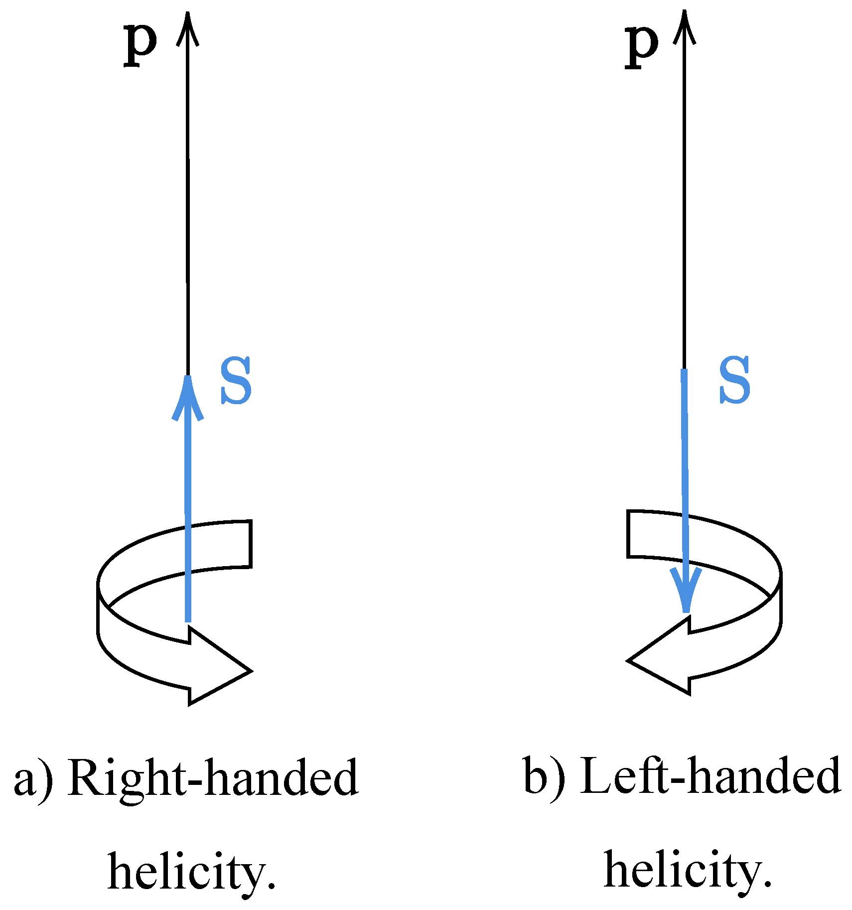
We will now study the manifestation of spin in the Dirac equation by analyzing the helicity of the possible solutions in the free particle. We can express the four bispinors that satisfy the Dirac equation and arise from our arbitrary choices. For positive energies, we have
while for negative energies
where the upper indices are linked to the sign of the energy and the lower ones are associated with the helicity. The calculation of the normalization factor N will be performed subsequently, following the discussion on the probabilistic interpretation of the Dirac equation.
Inserting Eqs. (98) and (99) into Eq. (82), we can obtain the solutions associated with each bispinor, which are given by
One may ponder whether it is permissible to discard negative-energy solutions, deeming them physically unacceptable. The answer to that is in the negative, as a quantum system requires a complete set of linearly independent states, and positive-energy solutions alone do not suffice. For the same reason, we cannot attempt to construct solutions solely with positive-energy bispinors, i.e., assuming , as this would result in dependent bispinors.
In Eqs. (98) and (99), the lower subscripts R and L were not properly explained. These subscripts are associate with the inherent helicity associated with each bispinor. To explore this characteristic, we must discuss the notion of operators again. In contemporary quantum mechanics, operators can be represented by matrices operating on states, represented by column matrices. We can leverage this notation to facilitate our interpretation.
For the spin operator , it is expressed as
where
When the operator acts on a state, it performs a measurement of spin, providing information concerning the spin of the given state. Similarly, when the Hamiltonian operator H acts on a state, it extracts information about the energy, for instance whether it is positive or negative. Hence, it becomes imperative to define a helicity operator, which, when acting on a state, provides information about the helicity of the corresponding state. This operator is expressed as
where the inner product represents the projection of spin onto the momentum. Therefore, when and are orthogonal, their inner product is zero.
The behavior of , in the case of free particle movement restricted to z is
that is, the projection of onto is precisely the component of the spin. We have for , according to Eq. (102),
so that the helicity operator measures the helicity of the solutions by the sign, positive or negative, of the elements along its diagonal when applied to a given state. For instance, for the state , we find
where the negative sign denotes negative helicity, commonly known as left-handed helicity. Applying the helicity operator to a positive, or right-handed, helicity solution would result in the constant () being multiplied by a positive sign. The distinct sign and its associated helicity confer the spin attribute to the respective solution. It is worth noting that we employ for simplicity in this example, but the same helicity would hold for since what holds significance is the sign acquired during the measurement process. Thus, the exponential term in does not affect the outcome of the measurement.
In summary, the action of the helicity operator provides information regarding the connection between momentum and spin. Positive helicity indicates parallel alignment between spin projection and momentum, while negative helicity signifies anti-parallel alignment. In the context of a free particle moving exclusively in the z direction, the projected spin component is precisely the spin in the z direction. By convention, we denote that right-handed helicity corresponds to spin up in this direction, whereas left-handed helicity corresponds to spin down.
Applying the helicity operator, as represented by Eq. (104), to the expressions given by Eqs. (98) and (99), leads to different helicities for both positive and negative energy solutions. For the positive energy solution , the result is right-handed helicity, while for , it yields left-handed helicity, as illustrated earlier. In the context of the non-relativistic limit, where the upper components have dominance, the coefficients and correspond to spin up and spin down, respectively. However, in the negative energy scenario, the application of (104) projects the right-handed helicity onto and the left-handed helicity onto . In the non-relativistic limit, and correspond to spin up and spin down, respectively.
Figure 6.
Illustrated depiction of helicity. In the left panel a) the alignment of momentum and spin in the same direction resulting in positive helicity, or right-handedness. Conversely, in the right panel b) the opposing directions of momentum and spin lead to negative helicity, or left-handedness. Adapted from Ref. [18].
Given that positive energy pertains to particles and negative energy pertains to antiparticles, we may put aside brevity in favor of a more explanatory notation of the solutions for a free particle. In the following, we will adopt the notation found in (100), applying our findings collectively to the states.
For didactic purposes, let us consider the following scenario: we are in possession of a free particle solution , but we do not know if it corresponds to a particle or antiparticle, nor its spin. However, we know that the state is associated with a electron or a positron. The process of discovering these two pieces of information is carried out through measurements, with energy H and helicity operators. This process is illustrated in Figure 7. Suggested as supplementary reading, the reference [80] provides an explicit derivation of solutions for the case of a free particle in three dimensions.
Having covered the energy of the free particle, the next step involves testing the continuity equation to determine whether the density can be defined as positive. We initiate this process by multiplying (78) by the conjugate transpose of , , obtaining
that we take the conjugate transpose as
Subtracting Eq. (109) from Eq. (108), we have
where we used the Hermitian property of and . Employing the product rule, we rewrite Eq. (110) as
Comparing the above equation with the continuity equation we conclude that
where is clearly positive definite since it is the sum of the squares of the magnitudes of the components of , which allow us to have an probability interpretation for . Furthermore, the probability current is defined as
It is common to use the notation resulting in
We can interpret Eq. (112) as the probability of finding a given particle in a certain region. If we consider a single particle restricted to a volume V, we rewrite it as
that we can use to calculate the normalization factor N of the free particle solutions. Taking the bispinor in Eq. (100) associated with as an example, we compute
where we isolate N to find the expression
which is the same normalization factor as the other solutions to the free particle problem.
The elucidation of plane wave solutions and their admissible negative energies, along with a viable probabilistic interpretation, underscores the strong aspects of Dirac’s model. However, the question remains: Does the Dirac equation derive the Pauli equation in the non-relativistic scenario?
6.1. Electromagnetic Interactions in the Non-Relativistic Limit
In this subsection, we will examine how the Dirac equation behaves in the presence of electromagnetic interactions within the non-relativistic limit, precisely with the aim of derive the Pauli equation. We start by incorporating the minimal coupling into Dirac Hamiltonian, as given in Eq. (52). This results in
Thus, applying H on , we obtain
where is an energy eigenvalue described as
where K is the kinetic energy, is the electric potential energy and is the rest energy. We can write this eigenvalue equation in its matrix form as
from which we can extract a system of two equations as follows. From the lower equation, we have
which can be approximated to
since, for positive energies, the kinetic and electric energy are much smaller than in the non-relativistic limit. Similarly, we can write the upper equation as
where , is the non-relativistic energy, that is, the total energy excluding the rest energy. Replacing Eq. (124) into Eq. (125), we obtain
Using the identity related to the the Pauli matrices products, we obtain
where we can rewrite the vector product by applying it to , i.e,
so that, Eq. (127) becomes
which is, precisely, the Pauli equation [see Eq. (57)] In this manner, it can be stated that the Pauli equation represents the non-relativistic limit of the Dirac equation, and the emergence of the Pauli matrices, linked to the spin, is a natural outcome of Dirac’s theory. In particular, the term represents the magnetic moment of the electron, incorporating the gyromagnetic ratio factor of , which had previously been assumed ad hoc.
6.2. Foldy-Wouthuysen Transformation
Another, more sophisticated, and general method for testing the non-relativistic limit of the Dirac equation exists. This approach is known as the Foldy-Wouthuysen (FW) transformation [81], introduced by Leslie Foldy and Siegfried Wouthuysen (and later generalized by Caze [82]), and we will delve into it in this subsection. Costella and McKellen argue that it is only through this method that a significant classical limit is achieved with respect to particles and antiparticles [83]. We have chosen to highlight this procedure because of its historical importance and the broad range of relevant applications. For instance, deriving the Dirac equation in a rotating frame must reduce to the Pauli equation in a rotating frame in the non-relativistic limit [84]. Additionally, we can connect the final result obtained with the FW transformation into the Dirac Hamiltonian with the Sommerfeld equation [see Eq. (35)] and the fine structure of hydrogen.
However, to accomplish this, we utilize a more demanding mathematical framework. Therefore, it is natural for a reader who has not encountered difficulties thus far to encounter them now. Furthermore, we will carry out this procedure in the case of interaction with an electromagnetic field. We will not delve into every step of the calculations due to their length, but this derivation can be found in more detail in the refs. [17,18].
As we saw in the free particle solution, the positive (negative) energy solutions have a large (small) components. The main concept of the FW transformation is to utilize this characteristic of the Dirac equation as a foundation for a new representation. For this purpose, the concept of parity is used.
An operator or matrix is even (odd) if it commutes (anti-commutes) with the parity matrix. In practice, an odd operator connects elements of opposite parity, while an even operator connects elements of similar parity. In the relativistic scenario, we can consider the example of the Dirac matrix , which “connects” - in this case, couples - the elements of positive and negative energy of the bispinor. On the other hand, the matrix is even, since it does not couple the positive and negative energy elements. Thus, we can rewrite the Dirac Hamiltonian as
where is the odd part of the Dirac Hamiltonian and is the even part. Thus,
Due to the parity property, we have the following relations:
Previously, we noted that our goal is to eliminate the odd component from the Hamiltonian, as it links the upper and lower sections of the bispinor. To achieve this, we apply a transformation in the Hamiltonian, ensuring that in the resulting form the odd component is no longer present. To do this, we define the operator
and during the derivation we perform unitary transformations of the type
where we have assumed that the field, and consequently, the vector potential and the Hamiltonian are time-independent. This unitary transformation is a FW transformation. The above equation should be understood in the light of a power series, using the Baker-Hausdorff lemma
where is the commutator between the operators L and A. Therefore, Eq. (134) becomes
when we consider terms up to the order of . We calculate the commutators separately, up to the desired order employing Eq. (132) as follows
For the odd part, it suffices to include terms up to the order of , and hence the third term in Eq. (139) can be neglected. In this way, we can rewrite Eq. (136) as
Now, considering that raised to even powers and are even, there are still odd terms in the equation. Therefore, we can rewrite it as
Thus, we write
The next step consists in applying the operator
so that the Hamiltonian in Eq. (141), after undergoing a second FW transformation, becomes
The third term in the above equation is odd, so it is necessary to perform a third FW transformation so that we obtain
where is given by
Using the relation and , with calculations similar to those applied in the previous subsection, we obtain
Taking the case of positive energy, we can replace and with their upper blocks
Thus, we obtain
The first three terms above represent the expansion of the kinetic energy , describing the increase in mass in the relativistic case. The next pair of terms is associated with magnetic dipole and electrostatic energy. Subsequently, the next two terms describe the spin-orbit (SO) interaction. For a spherically symmetric potential, we have . Additionally, we can write
so that the SO can be written as
Finally, The last term in Eq. (151) is called Darwin term, and it is associated with a purely relativistic effect, the Zitterbewegung effect, which translates to "trembling motion of the electron" from German, as coined by Schrödinger [85]. This steams from the interference between the positive- and negative-energy eigenstates.
In this new representation, the Hamiltonian contains terms from the Pauli equation, added to the relativistic terms and the SO interaction. The presence of these latter terms revisits an aspect mentioned earlier: the fine structure of hydrogen.
As mentioned previously, Schrödinger encountered difficulties in deriving Sommerfeld’s formula through his relativistic approach. If the Dirac equation indeed proves to be the suitable equation for describing quantum and relativistic phenomena, then Eq. (35) should be deducible from it. Initially, Dirac utilized a first-order approximation method akin to Pauli’s earlier approach. However, in 1928, Darwin [86] and Gordon [87] successfully obtained an exact solution, showcasing that the experimentally successful result of old quantum theory could be derived from a more formal representation.
Dirac published his theory in two papers, [1,2], the first of which was published in February. The effect of Dirac’s theory of the electron was revolutionary in quantum mechanics. Rosenfeld would call it a “miracle, an absolute marvel” [3]. From one of the biggest initial obstacles of the Dirac equation, the allowed negative energies came one of its greatest triumphs: the prediction of antiparticles. In 1931, as mentioned, Dirac conjectured an antiparticle to fill the sea of negativity, but there was no experimental proof. In 1933, however, Anderson [88] experimentally proved the existence of positrons, solidifying the Dirac equation as the most accurate equation for representation of spin 1/2 particles, a notion that endures in Relativistic Quantum Mechanics to this day.
7. Relativistic Covariant Notation
This section presents natural units and relativistic covariant notation as alternative approaches to express the KG and Dirac equations. Utilizing these methods will enable a more straightforward classification of how equations transform under Dirac transformations. Even though natural units and relativistic notation can be used separately, we opt to use them together here to improve the practical utility of the equations discussed. As mentioned in the Introduction, we aim to enhance the experience of exploring the KG and Dirac equations through these notations.
In natural units, physical constants serve as the units of associated physical quantities. Although this approach may appear arbitrary, its implications become evident in the expressions of various physical quantities. The speed of light , for example, can be used as a natural unit of speed, so that a speed of becomes , or , simply. Therefore, v becomes a dimensionless parameter, which we usually designate . Time, elementarily defined as , is measured in distance units. For the purposes of this work, we will use, in addition to , the normalized Planck constant . Using this we can write the KG (39) and the Dirac equation (78) respectively as
As mentioned earlier, in relativity, we deal with four dimensions: one temporal and three spatial, which can be interpreted as four components of a vector. Physical quantities composed of these four components are termed four vectors. We implicitly utilize this concept when discussing momentum, even though, at that point, we were not employing the covariant notation. There are two types of four-vectors: contravariant and covariant; this classification stems from differential geometry and will not be explored in this work. A generic contravariant four-vector is denoted by an upper index, being expressed as
where represents the three spatial components. We can write, following the most common notation,
where the Greek indices () run through and the Latin indices () go through . A contravariant four-vector has a dual covariant four-vector, symbolized with the lower index
where is the metric tensor in Minkowski space, suitable for special relativity, and expressed in covariant components as
In Eq. (158), we used Einstein sum notation,
where the repeated index symbolizes summation. Making the summation explicit and incorporating the chosen metric, is expressed as
A relevant operation with four-vectors is the inner product, exclusively applicable between a contravariant and a covariant four-vectors. Consider a generic covariant four-vector . The inner product between and is defined as
or, more specifically, in the case of as
Having defined the basic properties of the relativistic covariant notation, we can employ it to define physical quantities as four-vectors. The contravariant four-vector position is
with the inner product expressed as
The definition of the position contravariant four-vector allows us to write the four-gradient operator
which is covariant, even with the positive sign in the spatial coordinates. The contravariant dual is then defined as
with the inner product written as
We can also define a four-moment, in covariant form as
with the inner product expressed as
associated with the energy of a relativistic particle (36).
Now, let us employ the techniques outlined to rewrite and study the KG and Dirac equations from an alternative perspective. By substituting (168) into (154), we can express the KG equation as
In addition to providing an alternative way to write the equations, the relativistic covariant notation facilitates the analysis of invariance under Lorentz transformations. This happens because the equations expressed in this notation have the property of transforming predictably when the aforementioned transformations are applied. Instead of conducting a proper Lorentz transformation, which would involve introducing additional concepts, we will confine our analysis to a mathematical argument grounded in the space-time interval, whose definition will be introduced shortly.
When assessing the invariance of the Dirac equation under Lorentz transformations, we invoked the symmetry between time and space dictated by relativity, as evidenced by the derivative orders. This rationale is reinforced by the non-invariance of the Schrödinger equation (with time as a first-order derivative and space as a second-order derivative) and the invariance of the KG equation (featuring second-order derivatives in both time and space). An alternative route to the same conclusion involves considering the space-time interval , defined as
must be invariant [89,5]. Consequently, it can be inferred that the combination of derivatives, expressed in covariant notation as , remains constant when transitioning between inertial frames of reference.
Upon examination of equation (171), the presence of the inner product between the derivatives (168) and of the mass m becomes evident. The mass, being the rest mass, remains constant and does not alter with a change of reference frame. Furthermore, as we have just established, the inner product is invariant. Consequently, utilizing covariant relativistic notation allows for an immediate recognition of the invariance of the KG equation under Lorentz transformations.
Multiplying (155) by by the left and rewriting it with covariant notation results in
where we identify an inner product between the four-vector and the derivative (166), so that
where we again identify the mass and an inner product. The product in question is not directly related to the space-time interval (172), and its invariance cannot be assumed immediately. It is imperative to demonstrate that the inner product within the Dirac equation remains invariant. To establish this, we will extend our proof to encompass any pair of contravariant and covariant four-vectors, aiming to generalize the result for both the KG and Dirac equations. To commence, we initiate a one-dimensional Lorentz transformation, akin to equations (20) and (21), on two arbitrary four-vectors.
where in natural units. The other components remain the same, so the inner product after the Lorentz transformation is
where we use (22), which leads to
Here, we observe that the inner product between any two four-vectors remains constant, consequently ensuring the constancy of the Dirac equation. This observation also extends to the KG equation.
Furthermore, if one wishes to write the Dirac equation even more bluntly, Feynman notation, where , is employed, so that
To conclude the comparison between the equations, we present Table 1, aiming to encapsulate the most relevant characteristics of the models presented in this work.
8. Conclusions
In this work, we provided an introduction to the Dirac equation, placing particular emphasis on the historical context of its conception. In this context, we conducted comparisons with the Schrödinger and KG equations, focusing on their invariance under Lorentz transformations and energy eigenvalues.
We started with a historical preamble, illustrating that, in the 1920s: i) Physics was effervescent, marked by new discoveries in quantum mechanics, ii) a consensus on a consistent methodology had not yet been reached, and iii) Dirac was deeply involved in both previous aspects, actively contributing to the construction of the new physics. Moreover, we outlined features of matrix mechanics and underscored the significance of Dirac’s canonical quantization, which was found to be applicable in other instances in this study.
The natural course was to present wave mechanics as an alternative to matrix mechanics. Schrödinger’s equation enabled many physicists [32] to have a more practical view of quantum mechanics and, from it, Born was able to extract a probabilistic interpretation that originated from the density being positive definite. Furthermore, Schrödinger managed to solve the problem of the eigenvalues for the hydrogen atom, deriving the non-relativistic hydrogen spectra – a feat that matrix mechanics had not been able to accomplish without ad hoc hypotheses. However, Schrödinger equation is not invariant under the Lorentz transformation; it does not fit into relativity. We show its non-invariance explicitly, with a one-dimensional Lorentz transformation and without relativistic notation.
Subsequently, we introduced the KG equation. Initially conceived as a wave equation compatible with relativity principles, it fulfills this purpose by remaining invariant under Lorentz transformations. However, upon delving into the dynamics of the model for a free particle, we demonstrated that it permits solutions with negative energies. Moreover, the second-order time derivative impeded defining a density as positive, consequently preventing a probabilistic interpretation. Consequently, its physical applications were limited then, especially considering the lack of knowledge about spinless particles. The consideration of spin prompts us to focus on the subsequent wave equation: the Pauli equation.
Spin, the electron’s new degree of freedom, emerged to explain the quantization detected in SG’s experiment. Pauli forcibly inserted spin into Schrödinger’s equation, replacing the wave function with a spinor – a two-component column matrix – and including his matrices. Pauli successfully derived a precise equation applicable to the non-relativistic regime through this approach. Nevertheless, Pauli was unable to make progress regarding the integration of quantum mechanics and relativity.
Finally, we introduced the Dirac equation, marking the concluding chapter of the narrative we aimed to tell. Dirac, dissatisfied with the KG equation as the relativistic wave equation due to the second-order time derivative that hindered a probabilistic interpretation, sought a more fitting solution in line with his transformation theory. We presented a deduction of the equation from an elegant result found by Dirac, discussing the emergence of the matrices and the bispinor as evidence of yet another degree of freedom beyond the spin. It is noteworthy how matrices, seldom employed in Physics until the advent of matrix mechanics, arise naturally as inherent to the Dirac equation.
We encountered negative energy solutions once again after solving the dynamics for a free particle at rest. The deeper investigation into the physical significance of these energies unfolds when considering the case of a moving particle, where we have observed that the two upper components of the bispinor correspond to the particle, associated with positive energy, while the lower components correspond to an entity linked with negative energy. We commented on how Dirac’s conjecture, his sea of negative energy, explains this result and postulates, through a “hole” in the sea, the existence of an antiparticle. Helicity serves as an auxiliary means of interpreting these outcomes: Positive (right-handed) and negative (left-handed) helicity are imposed, respectively, on the first and second components of the upper part of the bispinor in the case of positive energy. For negative energy, the third component of the bispinor exhibits right-hand helicity, while the fourth component displays left-hand helicity. We have used these types of helicity to discern the spin of the solutions that emerge from the free-particle problem, just as we employed the sign of energy to differentiate between the particle and the antiparticle.
By analyzing the continuity equation for Dirac’s equation, we establish that the density is positive definite, allowing for a probabilistic interpretation. This characteristic, at the time, underscored the primacy of the Dirac equation over the KG equation. Additionally, we demonstrated that, in the non-relativistic limit, the Dirac equation yields the Pauli equation, naturally yielding the magnetic spin ratio. Furthermore, we commented on how the model manages to derive the Sommerfeld formula exactly. In this context, we have shown that terms associated with relativistic corrections and spin-orbit interaction appear by employing the FW transformation. Finally, we use relativistic covariant notation to show more concise forms of the KG and Dirac equations and, utilizing four-vectors, the invariance of Dirac’s model.
We recommend further reading of [14], which informatively elucidates how the initial incongruity between the Schrödinger equation and relativity gives rise to Quantum Field Theory (QFT) and underscores the pivotal role played by the Dirac equation in facilitating this transition.
Acknowledgments
This work was partially supported by the Brazilian agencies Conselho Nacional de Desenvolvimento Científico e Tecnológico (CNPq) and Instituto Nacional de Ciência e Tecnologia de Informação Quântica (INCT-IQ). It was also financed by the Coordenação de Aperfeiçoamento de Pessoal de Nível Superior (CAPES, Finance Code 001). F.M.A. acknowledges CNPq Grant No. 314594/2020-5. E.O.S. acknowledges CNPq Grant 306308/2022-3, FAPEMA Grants APP-12256/22 and UNIVERSAL-06395/22.
Appendix A. The Dimension of the Dirac Matrices
In this section, we discuss the dimension of Dirac matrices, utilizing the bra(c)ket notation introduced by Paul Dirac. Here, a ket represents a state and can be expressed as a vector within a specific Hilbert space. Every ket has a corresponding bra , representing the same state but originating from a Hilbert space dual to the ket’s space. Multiplying a ket by its corresponding bra yields
We start the discussion on the dimension of Dirac matrices from the assumption that we do not know any representation for and , only the algebra of the anticommutators (70) and
a relation that can be obtained by recalling the definition (69) and that (64). From the squaring of as functions of , as indicated in (69), we can similarly infer a relationship for , leading to
Through their anticommutator (70), we can write , so that (A3) becomes
Moreover, we have (64) and (A2), so that
Furthermore, we take and as Hermitian for being part of the Hamiltonian H (77).
To advance the discussion, we must analyze the diagonal elements of the matrices, a task we will undertake by employing the trace. The trace of a matrix A
is given by the sum of the elements on its diagonal
Interestingly, the trace does not change if we multiply the matrix A by a unitary matrix U on the right and by the respective conjugate transpose unitary matrix on the left
But, as they are Hermitian, therefore and , and we have the condition (A2), the matrices and are considered unitary, such that
Using (A8) for , multiplied the other component of and its conjugate transpose, and , such that
where we can use the anticommutation relation (70), concluding that , and that the trace is
Nevertheless, the product between the components in j is equal to the unit (A5) such that
which is only satisfied if the trace of is null
Repeating the same process for the matrix, we obtain
Now, let us analyze the action of on a state , which is an eigenstate of and, consequently, has the following eigenvalue relationship
where is the eigenvalue associated with .
Making the inner product between two of these eigenstates, as in (A1), we find
where we can insert , since they are equal to unity (A5), applying them individually on the states, obtaining
from where we conclude that
given that the eigenvalues of a Hermitian matrix are real. Another way to calculate the trace of a given matrix is precisely through its eigenvalues
where we use the index l to avoid confusion with the index i from the matrix . However, since the trace of is zero, the number of elements on the main diagonal and the dimension of the matrix must be even, and the same can be said for . For a dimension, the three Pauli matrices satisfy the anti-commutation relation (70). However, since Dirac needed four matrices, the minimum dimension for and is . Naturally, according to (69), the dimension of the gamma matrices is also .
References
- P. A. M. Dirac, Proc. R. Soc. Lond. A 117, 610 (1928a). [CrossRef]
- P. A. M. Dirac, Proc. R. Soc. Lond. A 118, 351 (1928b). [CrossRef]
- H. Kragh, Arch. Hist. Exact Sci. 24, 31 (1981). [CrossRef]
- G. Farmelo, It Must Be Beautiful: Great Equations Of Modern Science (Granta Books, 2002).
- A. Zee, Quantum field theory in a nutshell, 2nd ed. (Princeton University Press, 2010).
- T. Ohlsson, Relativistic Quantum Physics: From Advanced Quantum Mechanics to Introductory Quantum Field Theory (Cambridge University Press, 2011). [CrossRef]
- A. H. C. Neto, F. A. H. C. Neto, F. Guinea, N. M. R. Peres, K. S. Novoselov, and A. K. Geim, Rev. Mod. Phys. 81, 109 (2009). [CrossRef]
- K. S. Novoselov, A. K. K. S. Novoselov, A. K. Geim, S. V. Morozov, D. Jiang, M. I. Katsnelson, I. V. Grigorieva, S. V. Dubonos, and A. A. Firsov, Nature 438, 197 (2005). [CrossRef]
- E. Corchero, Astrophys. Space Sci. 275, 259 (2001). [CrossRef]
- I. Tutusaus, B. Lamine, A. Dupays, and A. Blanchard, Astron. Astrophys. 602, A73 (2017). [CrossRef]
- PBS Space Time, Anti-Matter and Quantum Relativity | Space Time (2017).
- Ciência Todo Dia, Ciência todo dia: Ondas gravitacionais: O que são e como são detectadas.
- A. Smirnov and A. J. D. F. Jr., Rev. Bras. Ens. Fis. 38, (2016). [CrossRef]
- R. Thibes, Rev. Bras. Ens. Fis. 44, (2022). [CrossRef]
- G. Rajasekaran, Resonance 8, 59 (2003). [CrossRef]
- A. Pais, Inward Bound, 1st ed., Vol. 1 (Oxford University Press, 1988). [CrossRef]
- J. D. Bjorken and S. D. Drell, Relativistic Quantum Mechanics (McGraw-Hill Book Company, 1964).
- W. Greiner, Relativistic Quantum Mechanics. Wave Equations, 3rd ed. (Springer Berlin, Heidelberg, 2000). [CrossRef]
- P. A. Tipler and R. Llewellyn, Modern Physics, 6th ed. (W. H. Freeman, 2012).
- A. A. Levy, Am. J. Phys. 53, 454 (1985). [CrossRef]
- J. Bernstein, Am. J. Phys. 73, 999 (2005). [CrossRef]
- K. Gottfried, Am. J. Phys. 79, 261 (2011). [CrossRef]
- W. Heisenberg, Z. Phys. 33, 879 (1925). [CrossRef]
- M. Jammer, The Conceptual Development of Quantum Mechanics, 2nd ed. (American Institute of Physics, 1989).
- A. Pais, Subtle Is the Lord: The Science and the Life of Albert Einstein, 1st ed. (Oxford University Press, 1982).
- M. Born and P. Jordan, Z. Phys. 34, 858 (1925). [CrossRef]
- M. Born, W. Heisenberg, and P. Jordan, Z. Phys. 35, 557 (1926). [CrossRef]
- K. Helge, Dirac: A Scientific Biography, 1st ed. (Cambridge University Press, 1990).
- P. A. M. Dirac, Proc. R. Soc. Lond. A 109, 642 (1925). [CrossRef]
- M. Born, My Life: Recollections of a Nobel Laureate (Scribner, 1978).
- W. Pauli, Z. Phys. 36, 336 (1926). [CrossRef]
- M. Beller, Isis 74, 469 (1983). [CrossRef]
- E. Schrödinger, Ann. Phys. (Berl.) 384, (1926a). [CrossRef]
- E. Schrödinger, Ann. Phys. (Berl.) 384, (1926b). [CrossRef]
- E. Schrödinger, Ann. Phys. (Berl.) 385, (1926c). [CrossRef]
- E. Schrödinger, Ann. Phys. (Berl.) 186, (1926d). [CrossRef]
- J. Quaglio, Rev. Bras. Ens. Fis. 43, (2021). [CrossRef]
- E. Schrödinger, Ann. Phys. (Berl.) 384, 734 (1926e). [CrossRef]
- M. Born, Z. Phys. 38, 803 (1926). [CrossRef]
- P. A. M. Dirac, Proc. R. Soc. Lond. A 112, 661 (1926). [CrossRef]
- P. A. M. Dirac, Proc. R. Soc. Lond. A 113, 621 (1927). [CrossRef]
- J. J. Sakurai and J. Napolitano, Modern Quantum Mechanics, 3rd ed. (Cambridge University Press, 2020). [CrossRef]
- D. J. Griffiths and D. F. Schroeter, Introduction to Quantum Mechanics (Cambridge University Press, 2018). [CrossRef]
- R. P. Feynman, R. B. Leighton, and M. Sands, The Feynman Lectures on Physics, Vol. III: The New Millennium Edition: Quantum Mechanics, 50th ed., Vol. 3 (Basic Books, 2013).
- R. Eisberg and R. Resnick, Quantum Physics of Atoms, Molecules, Solids, Nuclei, and Particles, 2nd ed. (John Wiley & Sons, 1985).
- M. Planck, The Universe in the Light of Modern Physics, 1st ed. (Norton, 1931).
- S. T. Thornton and J. B. Marion, Classical Dynamics of Particles and Systems, 5th ed. (Brooks/Cole, 2004).
- H. Padmanabhan and T. Padmanabhan, Phys. Rev. D 84, 085018 (2011). [CrossRef]
- D. Home, Conceptual Foundations of Quantum Physics: An Overview from Modern Perspectives (Springer US, 1997). [CrossRef]
- A. Sommerfeld, Ann. Phys. (Berl.) 356, 1 (1916). [CrossRef]
- K. Barley, J. Vega-Guzmán, A. Ruffing, and S. K. Suslov, Phys.-Uspekhi (2021). [CrossRef]
- O. Klein, Z. Phys. 37, 895 (1926). [CrossRef]
- V. Fock, Z. Phys. 39, 226 (1926). [CrossRef]
- T. de Donder and F. H. van den Dungen, C. R. Acad. Sci. 183, 22 (1926).
- J. Kudar, Ann. Phys. (Berl.) 81, (1926). [CrossRef]
- W. Gordon, Z. Phys. 40, 117 (1926). [CrossRef]
- O. A. Tretyakov and O. Akgun, Prog. Electromagn. Res. 105, 171 (2010). [CrossRef]
- K. Elgaylani, M. Abd Allah, K. Haroun, M. Eisa, and A. Al Amer, Int. J. Phys. Sci. 2, 015 (2014).
- H. Fesbach and F. Villars, Rev. Mod. Phys. 30, 24 (1958). [CrossRef]
- O. Stern and W. Gerlach, Z. Phys. 9, 349 (1922). [CrossRef]
- W. Pauli, Sci. Nat. 12, 741 (1924). [CrossRef]
- G. E. Uhlenbeck and S. A. Goudsmit, Sci. Nat. 13, 953 (1925). [CrossRef]
- W. Pauli, Z. Phys. 43, 601 (1927). [CrossRef]
- W. Greiner, Quantum Mechanics: An Introduction, 3rd ed. (Springer Berlin Heidelberg, 1994). [CrossRef]
- W. L. Bade and H. Jehle, Rev. Mod. Phys. 25, 714 (1953). [CrossRef]
- C. G. Darwin, Proc. Roy. Soc. A116, 227 (1927a). [CrossRef]
- C. G. Darwin, Proc. R. Soc. Lond. A 115, 1 (1927b). [CrossRef]
- E. P. Wigner, Group Theory and its Application to the Quantum Mechanics of Atomic Spectra (Academic Press Inc., 1959).
- V. Bargmann, J. Math. Phys. 5, 862 (1964). [CrossRef]
- P. A. M. Dirac, Soviet Physics Uspekhi 22, 648. [CrossRef]
- B. Thaller, The Dirac Equation (Springer Berlin Heidelberg, 1992). [CrossRef]
- O. Klein, Z. Phys. 53, 157 (1929). [CrossRef]
- O. Klein and Y. Nishina, Z. Phys. 52, 853 (1929). [CrossRef]
- P. A. M. Dirac, Proc. R. Soc. Lond. A 126, 360 (1930). [CrossRef]
- J. R. Oppenheimer, Phys. Rev. 35, 562 (1930). [CrossRef]
- H. Weyl, Z. Phys. 56, 330 (1929). [CrossRef]
- P. Dirac, Proc. R. Soc. Lond. A 133, 60 (1931). [CrossRef]
- R. P. Feynman, Phys. Rev. 74, 939 (1948). [CrossRef]
- E. C. G. Stueckelberg, Helv. Phys. Acta 15, 23 (1942).
- S. M. Neamtan, Am. J. Phys. 20, 450 (1952). [CrossRef]
- L. L. Foldy and S. A. Wouthuysen, Phys. Rev. 78, 29 (1950). [CrossRef]
- K. M. Case, Phys. Rev. 95, 1323 (1954). [CrossRef]
- J. P. Costella and B. H. J. McKellar, Am. J. Phys. 63, 1119 (1995). [CrossRef]
- M. Matsuo, J. Ieda, E. Saitoh, and S. Maekawa, Phys. Rev. B 84, 104410 (2011). [CrossRef]
- E. Schrödinger, Sitz. Preuss. Akad. Wiss. Phys.-Math. Kl. 24, 418 (1930).
- C. G. Darwin, Proc. R. Soc. Lond. A 118, 654 (1928). [CrossRef]
- W. Gordon, Z. Phys. 48, 11 (1928). [CrossRef]
- C. D. Anderson, Phys. Rev. 43, 491 (1933). [CrossRef]
- L. D. Landau, The classical theory of fields, Vol. 2 (Elsevier, 2013).
Figure 1.
Not to scale timeline concerning the most relevant events for this work.
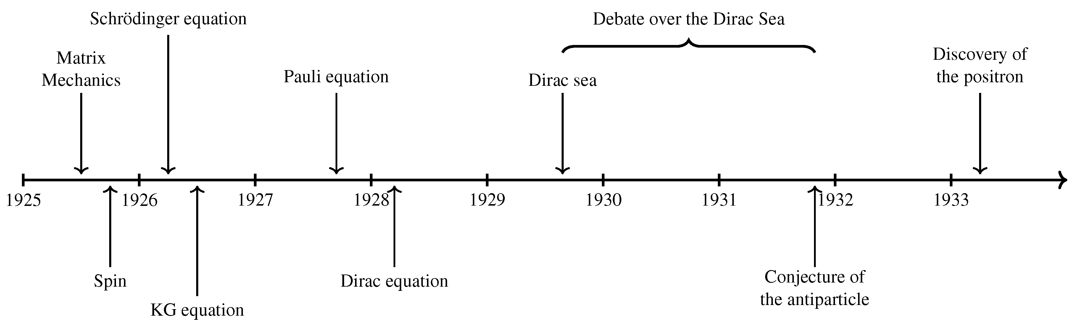
Figure 2.
Schematic representation of and for the scenario of a particle in a box of length L, a simple solution to the Schrödinger equation. Adapted from Ref. [19,233].
Figure 2.
Schematic representation of and for the scenario of a particle in a box of length L, a simple solution to the Schrödinger equation. Adapted from Ref. [19,233].
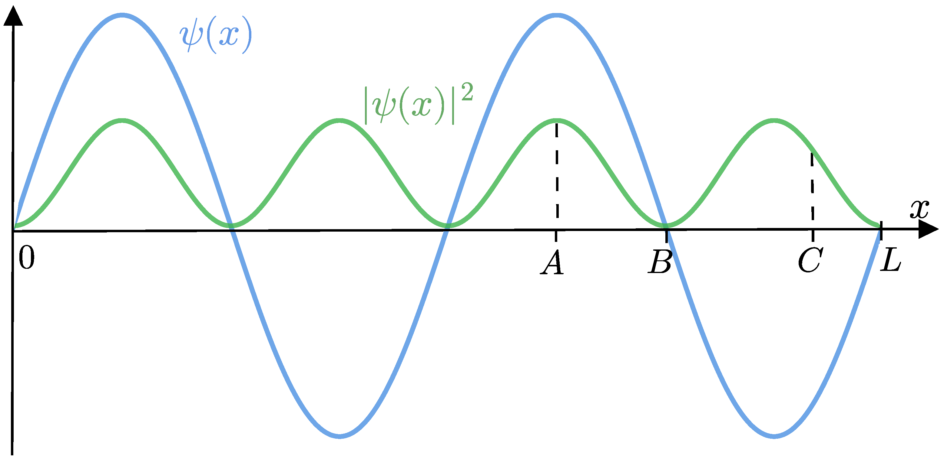
Figure 3.
The inertial frames and . Adapted from Ref. [47].
Figure 3.
The inertial frames and . Adapted from Ref. [47].
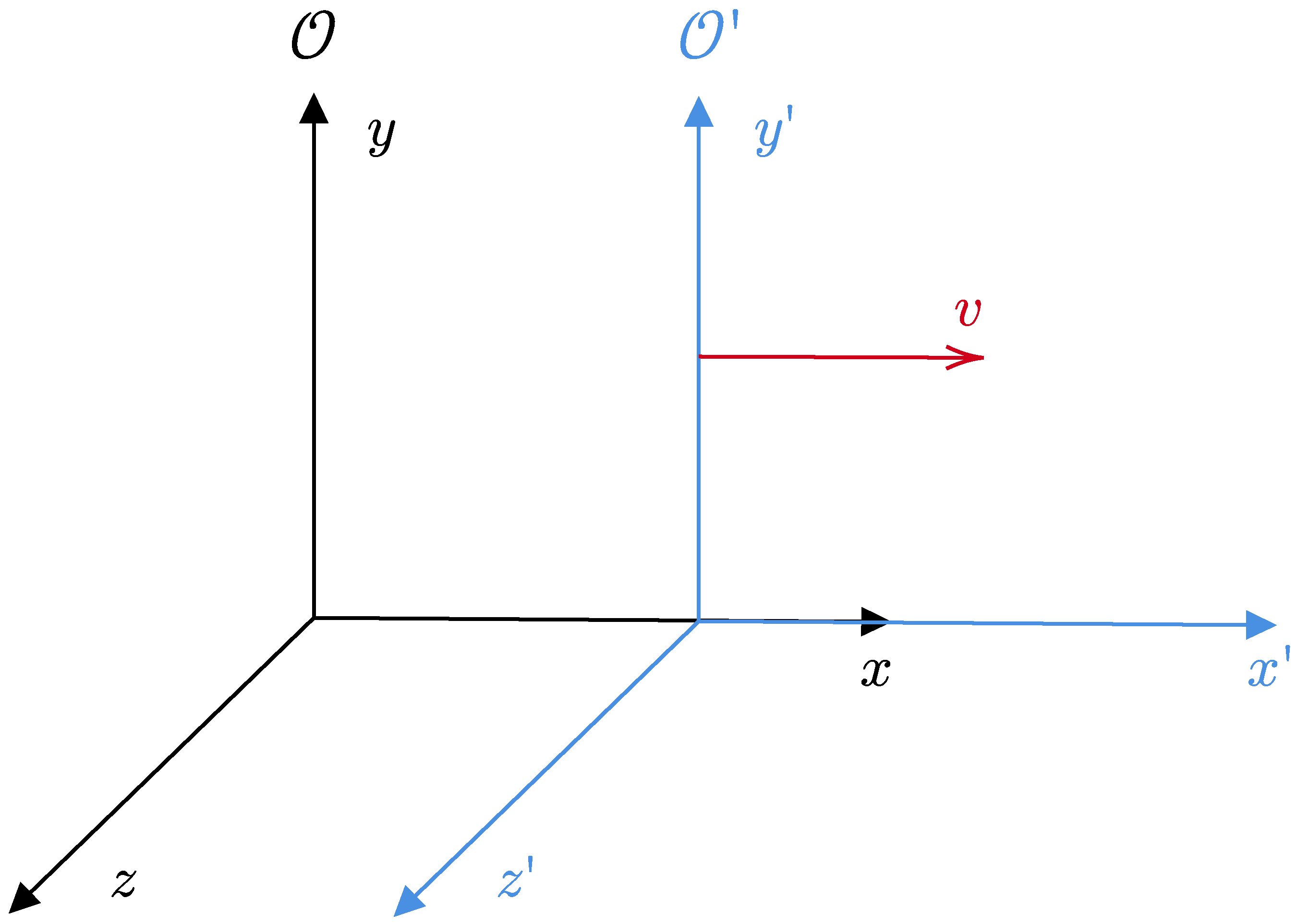
Figure 4.
SG experiment illustrated schematically. The beam of silver atoms is expelled from the furnace, passes through a collimator, and is subjected to a heterogeneous magnetic field . In the detector, two preferential regions are perceived. Adapted from Ref. [42,2].
Figure 4.
SG experiment illustrated schematically. The beam of silver atoms is expelled from the furnace, passes through a collimator, and is subjected to a heterogeneous magnetic field . In the detector, two preferential regions are perceived. Adapted from Ref. [42,2].
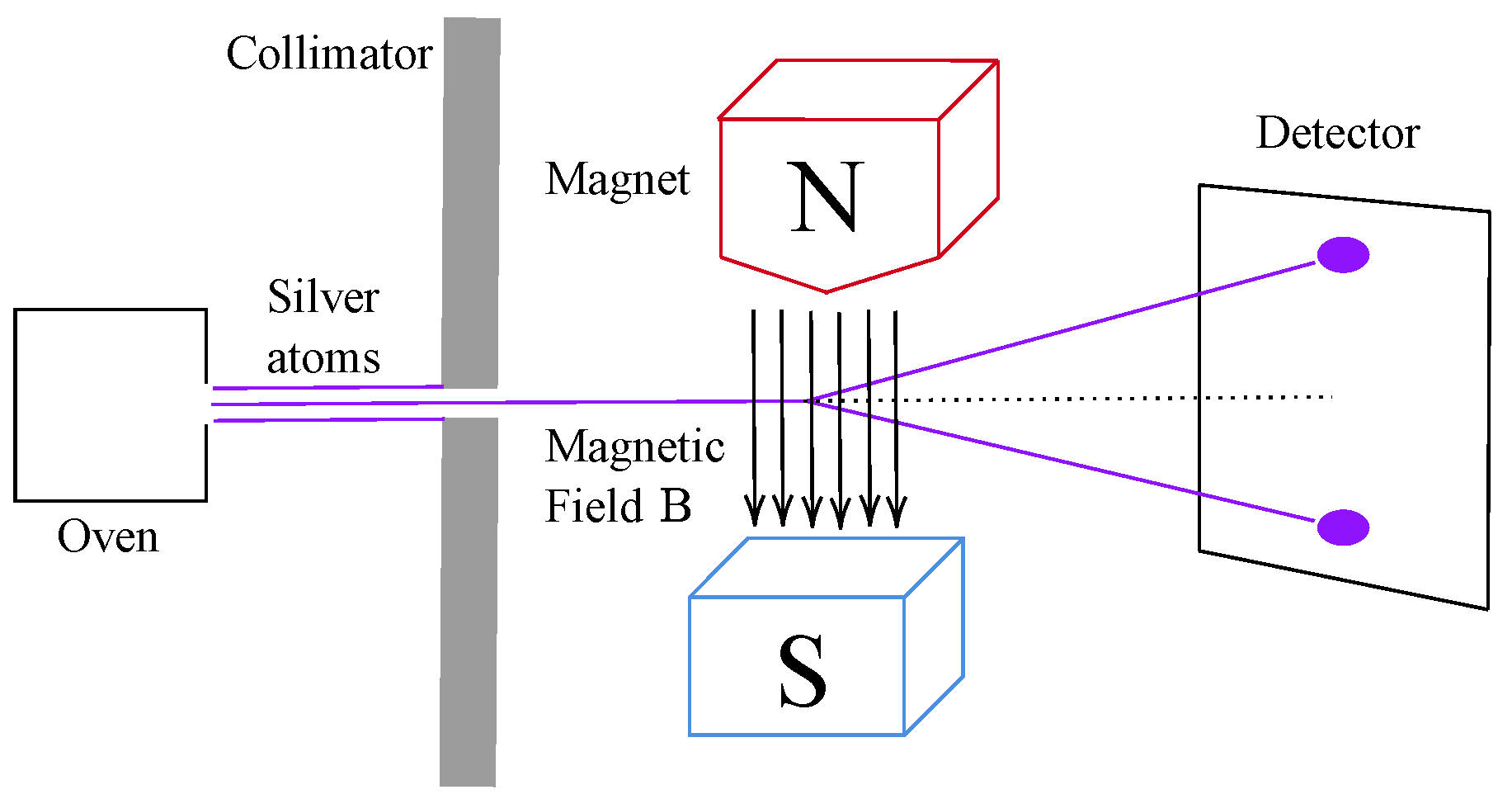
Figure 5.
Dirac equation’s energy diagram. Adapted from Ref. [42].
Figure 5.
Dirac equation’s energy diagram. Adapted from Ref. [42].
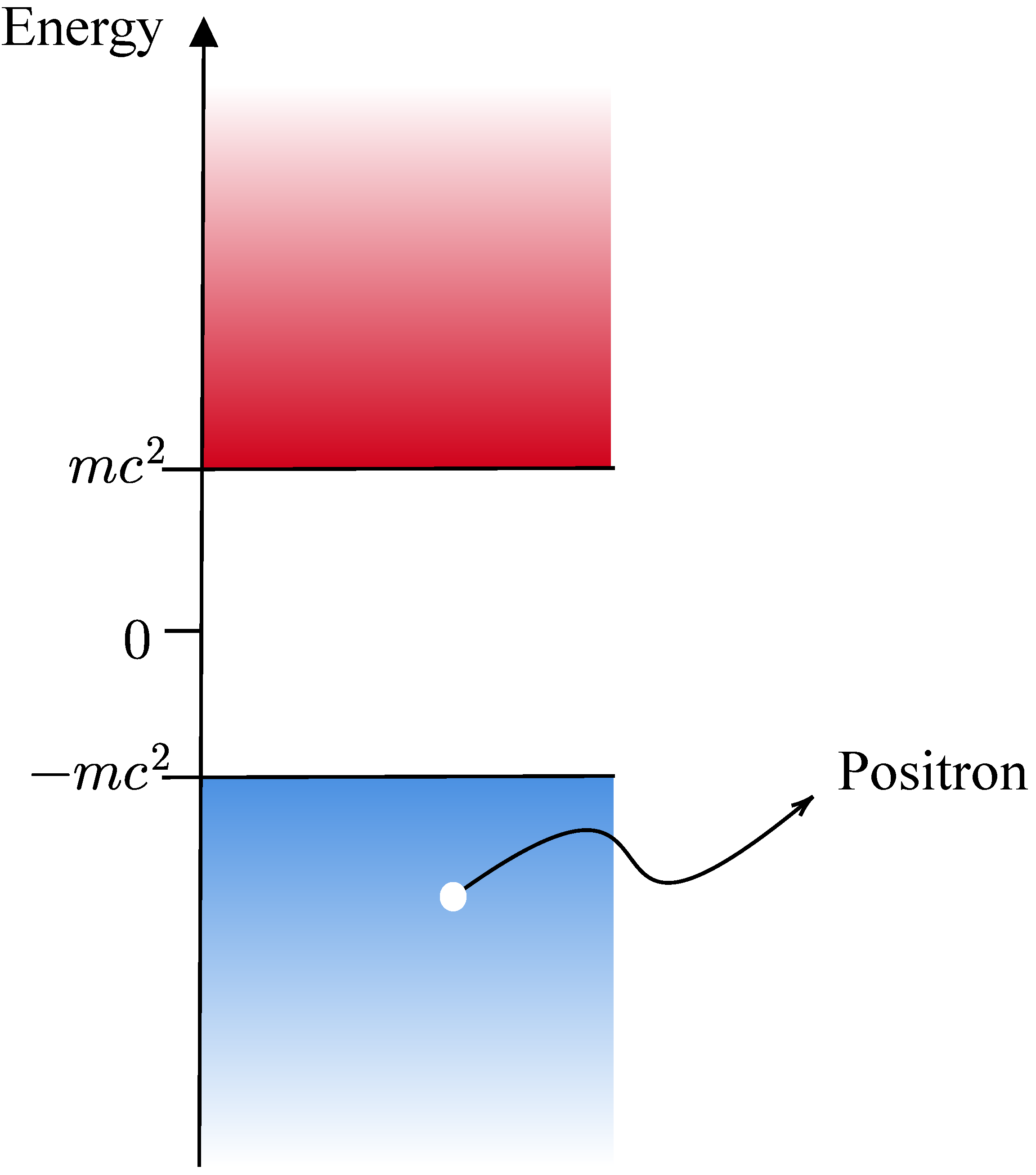
Figure 7.
Illustration of the measurement energy and helicity of a given solution of the free particle situation. The measurement is performed on a state for which we initially do not know the sign of the energy or the type of helicity.
Figure 7.
Illustration of the measurement energy and helicity of a given solution of the free particle situation. The measurement is performed on a state for which we initially do not know the sign of the energy or the type of helicity.
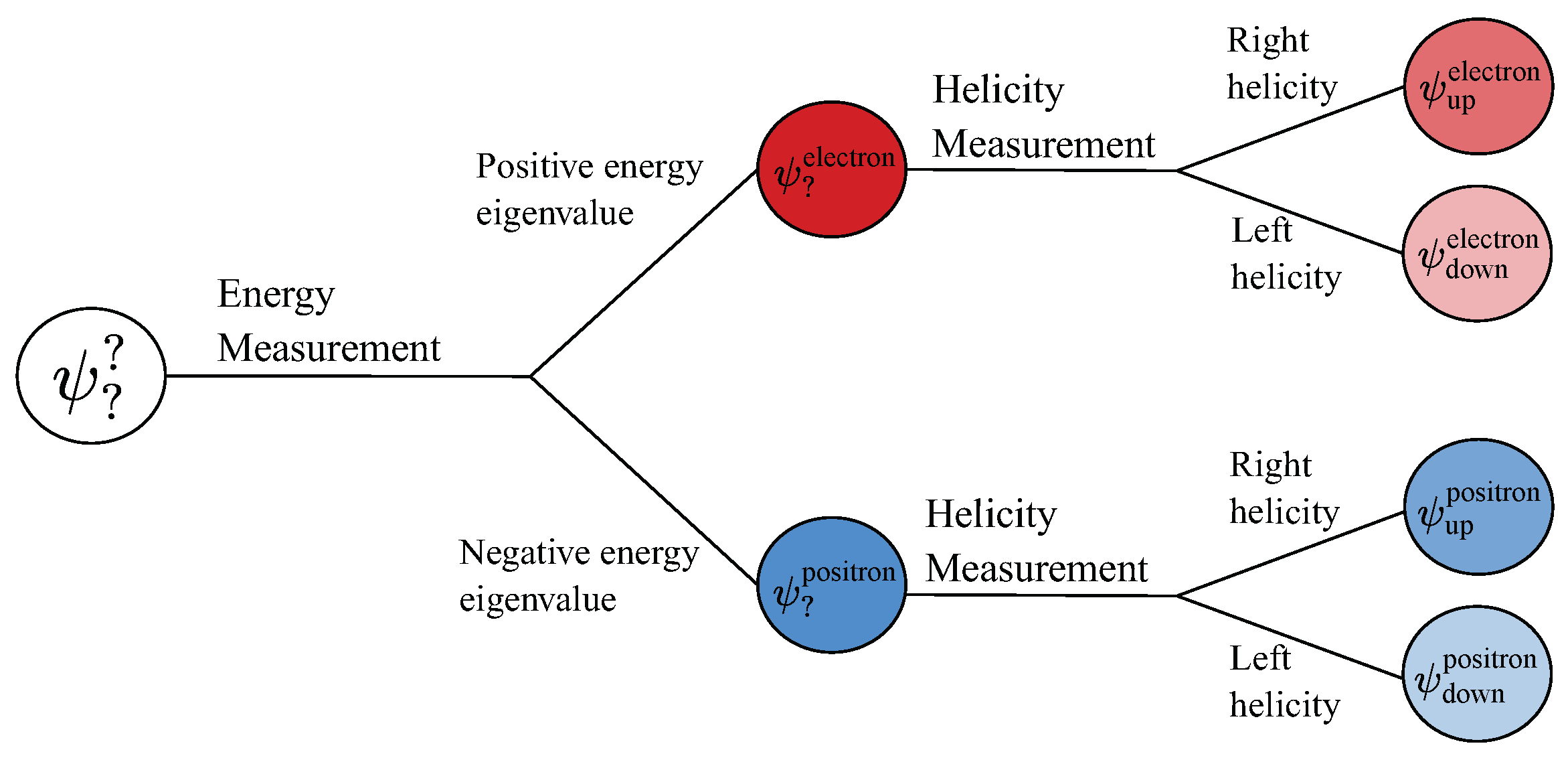

Table 1.
Table comparing the Schrödinger, KG, and Dirac equations regarding the aspects addressed in this article.
Table 1.
Table comparing the Schrödinger, KG, and Dirac equations regarding the aspects addressed in this article.
| Feature | Schrödinger | Klein-Gordon | Dirac |
|---|---|---|---|
| Equation | |||
| Energy | Only positive eigenvalues. | Both positive and negative energies are allowed. | Both positive and negative energies are allowed. |
| Probabilistic interpretation | Viable, since . | Not viable since is not positive definite. | Viable, since . |
| Relativity | Not-invariant under Lorentz transformation. | Invariant under Lorentz transformation. | Invariant under Lorentz transformation. |
| Spin | Does not contain spin. | Does not contain spin. | Contains the spin. |
Disclaimer/Publisher’s Note: The statements, opinions and data contained in all publications are solely those of the individual author(s) and contributor(s) and not of MDPI and/or the editor(s). MDPI and/or the editor(s) disclaim responsibility for any injury to people or property resulting from any ideas, methods, instructions or products referred to in the content. |
© 2025 by the authors. Licensee MDPI, Basel, Switzerland. This article is an open access article distributed under the terms and conditions of the Creative Commons Attribution (CC BY) license (http://creativecommons.org/licenses/by/4.0/).
Copyright: This open access article is published under a Creative Commons CC BY 4.0 license, which permit the free download, distribution, and reuse, provided that the author and preprint are cited in any reuse.


