
Submitted:
11 April 2025
Posted:
14 April 2025
You are already at the latest version
Abstract
This paper examines the relationship between stock prices, energy prices and climate policy uncertainty using 11 sectoral stocks in the US market. Evidence confirms that rising prices of energy commodities positively affect not only the energy & oil sector stocks but also create spillover effects across other sectors. Notably, all sectoral stocks, except those in real estate, show resilience to increases in crude oil and gasoline, suggesting potential hedging benefits. The findings reveal that sectoral stock returns are generally negatively affected by several types of uncertainty, including climate policy uncertainty, economic policy uncertainty, and oil price uncertainty, as well as energy & environmental regulation induced equity market volatility and the energy uncertainty index. These adverse effects hold across sectors, with few exceptions. Evidence reveals that the feedback effect between climate policy uncertainty changes and oil price changes produces an adverse impact on stock returns. Omitting these uncertainty factors from analyses could lead to biased estimates in the relationship between stock and energy prices.
Keywords:
uncertainty hypothesis
; energy uncertainties
; sectoral stock returns
; climate policy uncertainty
; oil prices
1. Introduction
This study is motivated by two empirical research streams on the US sectoral stocks: the first is whether changes in oil-related prices constitute an information content in explaining the US stock performance; the second is whether recently developed uncertainty indices can shed more light on the measure of risk and returns in the sectoral markets. Turning to the first stream of inquiry, this strand finds that an increase in oil prices has a positive impact on oil related stocks [1,2]. Sadorsky [3] reports that a rise in Canadian oil price factor leads to a higher stock returns in Canadian oil & gas industry. Boyer and Filion [4] further support that an increase in oil prices has a positive effect on the oil & gas stock prices in the Canadian market. Nandha and Faff [5] document that a rise in oil prices has a significant effect on stock returns in all sectors except the mining and oil & gas industries.
Hamilton [6] observes that a rise in oil prices has a significant impact on U.S. economic recessions for the postwar periods. Hwang and Kim [7] also find that oil price shocks lead to stock market variations in U.S. recessions. The evidence is consistent with the findings by Jones and Kaul [8], who find stock returns are negatively related to oil price rises. Literature along this line has been established in connecting the impact of oil prices to macroeconomic activities. It follows that an increase in oil prices can raise production costs and reduce household consumption, leading to lower demand for goods and services and, consequently, lower profits. The negative oil-return and stock return relationship is tied to the nature of the unpredictability of changes in oil prices and shocks to the underlying oil supply and demand as argued by Kilian [9], Kilian and Park [10] and Kang et al. [11]. As a result, the analysis of the oil-stock relationship depends on the way in which negative news affects changing economic expectations, market conditions and attitudes toward risk for future oil consumption.
As mentioned previously, the second stream of inquiry concerns what is the best measure of risk to explain the risk-oil return relation in the energy-oil sector based on recently developed indices of measuring uncertainty [12,13,14]. An empirical study by Diaz et al. [15] demonstrates that increased oil price volatility negatively affects G7 stock markets, while accounting for a structural break in 1986 identified in previous research. Liu et al. [16] show that oil price volatility causes a negative influence on stock returns. Behera and Rath [17] use G20 countries as their sample to examine the interconnectedness between crude oil prices and stock returns and confirm that volatility spillover exists from average oil prices to individual stock returns. Le and Luong [18] also find that in the US oil price and investor sentiment are net transmitters of shocks, and the stock market return is the net recipient.
However, Alsalman [19] examines the impact of oil price uncertainty on U.S. real stock returns by using a bivariate GARCH-in-mean VAR model and finds that oil price volatility does not have a statistically significant effect on U.S. stock returns. The absence of an uncertainty effect can potentially be attributed to companies' tendency to hedge against oil price fluctuations [19]. Another reason is that the GARCH-M model per se is merely based on a time series analysis by exploiting the historical pattern to predict the conditional variance in explaining stock returns. Thus, the GARCH-M model is incapable of exploring the driving forces behind the price volatility. However, using the econometric approach such as GARCH family models in fact excludes other information by merely focusing on price factors and would be more likely to commit a missing variable problem.
Recent empirical studies indicate that oil price shocks and economic policy uncertainty (EPU) are two major drivers of macroeconomic disturbance and financial market volatility [11,20]. Adekoya et al. [21] compare the impacts of EPU, VIX and OVX (Crude Oil Volatility index) on the stock returns of energy stocks and find that EPU has a stronger influence. The studies on how uncertainties shape the stock markets [22,23,24] document that EPU has a negative effect on stock returns. Moreover, Batten et al. [25] and Lin and Bai [26] show that the oil price has a negative response to the EPU. Liu et al. [16] uncover that the negative impact of oil volatility on stock returns is more profound as EPU interacts with the oil volatility, forming a nonlinear impact.
Despite its validity for using the concept of uncertainty, the information content of EPU mainly reflects a macroeconomic effect [6] rather than providing a direct measure of energy-specific uncertainty. Firstly, in light of recent advances in textual analysis for measuring uncertainties, that have motivated this paper to examine sectoral stock returns by utilizing energy-specific uncertainty factors. These include equity market volatility calibrated to energy and regulation, [27]; oil price uncertainty, OPU [13] and energy uncertainty index, EUI [14] and change in climate policy uncertainty, CPU [28]. These indices are constructed by using methodology proposed by Baker et al. [29] in measuring Economic Policy Uncertainty (EPU). A special feature of these uncertainty indices reflects news of forward-looking information collected, compiled, and reported by journalists. By incorporation of these uncertainty indices into the model, it allows us to verify the impact on the investor behavior and industrial reaction and hence to stock prices.
Secondly, this study examines alternative measures of energy prices and evaluates their impact on stock returns. While oil price, is commonly used in the empirical analysis, little attention has been given to the uses of alternative prices, such as gasoline price, , in modeling the test equation.
Third, the key argument that the interaction between changes in oil prices and climate policy uncertainty (CPU) was excluded from the model specification. An increase in oil prices often reflects an advancement in economic activity, which is associated with a higher demand for fuel combustion, thereby leading to increased greenhouse gas (GHG) emissions and rising global temperatures. As a result, changes in CPU are likely to be implemented to control emissions. Therefore, the interaction between changes in CPU and changes in oil prices is likely to affect stock returns. This gap should be addressed in literature.
The attempt of this study is to combine both uncertainty factors and energy related price changes into a framework to examine 11 sectoral stock returns in the US market. As a result, the model is more encompassing of using a set of key arguments in explaining stock returns. This study achieves several empirical findings. First, evidence shows that stock returns in the energy sector are negatively correlated with EUI and CPU. This negative relationship also holds in other sectors, suggesting that increases in uncertainty generally have an adverse effect on sectoral stock returns. Minor exceptions include positive signs in the Utility, Technology, Telecommunication or Real Estates sectors, implying that high uncertainty from energy-related sources can be hedged by the stocks in these sectors. These results are robust when real stock returns and excess stock returns are respectively used as the dependent variables in the analysis.
Second, the change in CPU on stock returns are nonlinear. This study finds evidence that the interacting term from change in CPU and oil price change on stock returns is significantly negative with a time lag. The exception is the Real Estate sector, which exhibit a positive sign. The negative effect of the interacting terms suggests a damage effect can arise from the feedback between CPU and oil price change.
Third, the model exhibits various performances with respect to different sectors. It is apparent that the uncertainty factors more effectively explain the stock returns in the Energy & Oil and Industrial sectors, which rely heavily on energy and oil as production inputs. In contrast, the impacts of uncertainties on the stock returns in the Utility, Technology, Telecommunication and Real Estates sectors are minimal.
Fourth, evidence consistently shows that the change in climate policy uncertainty reveals a negative effect on all sectoral stock returns, reflecting a market phenomenon that an increase in climate policy uncertainty will result in damaging losses to economic activity and the added costs of carbon that lead to jeopardizing the future stock performance.
Fifth, the changes in energy related commodity prices, including and , have significantly positive effects in explaining sectoral stock returns. The energy sector appears to be more sensitive and profoundly affected by the changes compared to other sectors. This means that with a few exceptions, companies in these sectors have the ability to pass energy prices to their stock price appreciation, implying a relative low demand elasticity with respect to upward shifts in prices in most sectors. The exception is the Real Estate sector, where the stock returns are negatively related to a rise in gasoline prices and insignificant to oil prices. The robust results are achieved by using different energy prices to explain stock returns. 1
Sixth, the stock returns during the 2008 global financial crisis and the 2020-2021 COVID-19 pandemic exhibited significant downturns. The use of dummy variables to account for these periods helps mitigate estimation biases [30,31].
The remainder of this paper is organized as follows. Section 2 provides a brief review of the literature on the relationship between stock returns and their determinants. Section 3 introduces a GED-GARCH model to examine these relationships. Section 4 describes the data and related variables in this study. Section 5 presents the estimated equations and robustness tests. Section 6 offers further evidence by examining the direct changes in climate policy uncertainty and indirect effect on stock returns. Section 7 summarizes the paper and discusses its implications.
2. Literature Review
A substantial amount of literature has been devoted to investigating the relationship between stock returns and oil price changes. Sadorsky [32] applies an unrestricted VAR model with GARCH effects to examine the U.S. monthly data and shows a significant correlation between oil price changes and aggregate stock returns. Sadorsky [3] and Boyer and Filion [4] report that increases in oil prices positively affect the stock returns of Canadian oil and gas companies. El-Sharif et al. [33] examine the relationship between oil price changes and stock returns in the UK oil and gas sector, finding a significant positive correlation. However, for the non-oil and gas sectors, the link between stock returns and oil price changes is weak. Hammoudeh and Li [1] show that oil price growth leads to a rise in the stock returns of the oil-exporting countries and US oil-sensitive industries. Ramos and Veiga [34] show that oil prices have a positive influence on market returns of the oil and gas industry around the world. Agarwalla et al. [35] discover that crude oil price has a significant positive influence on India stock price. 2
Contrasting evidence, however, is also present in the literature. For instance, Kling [36] finds that crude oil price increases lead to stock market declines. Jones and Kaul [8] use a cash flow dividend valuation model and yield negative relationships between stock returns and oil price changes in the U.S. and Canada. However, evidence from the U.K. and Japanese markets is not impressive. Park and Ratti [37] demonstrate that oil price shocks have a negative effect on oil stock returns in the U.S. and 13 European oil-importing countries. Maghyereh and Awartani [38] use a GARCH-M in VAR model and emphasize that oil uncertainty is a vital factor in determining stock returns. Their findings indicate that oil uncertainty significantly affects real stock returns negatively, concluding that there is a negative and significant relation between oil price uncertainty and real stock returns in all countries under consideration.
Evidence also shows mixed results regarding the relationship between stock returns and oil price changes due to different price sensitivity in different sectors or during different business conditions. In their analysis of sectoral stocks, Faff and Brailsford [39] find significant positive oil price sensitivity in the Oil and Gas and Diversified Resources industries, but significant negative sensitivity in the Paper and Packaging, and Transport industries. Nandha and Faff [5] analyze 35 DataStream global industry indices and conclude that increases in oil prices negatively affect equity returns across all sectors, except for mining, and oil & gas industries. Cong et al. [40] investigate Chinese data using a vector autocorrelation model and report that oil price changes do not produce a significant impact on sectoral stock returns except for manufacturing index and some oil companies. Using a bivariate VAR-GARCH-in-mean model, Caporable et al. [41] analyze Chinese sectoral stocks and find that oil price volatility generally boosts stock returns during demand-side shocks, except in the Consumer Services, Financials, and Oil & Gas sectors. However, during supply-side shock periods, the Financials and Oil & Gas sectors show negative reactions to oil price risk.
Lee and Chiou [42] examine the relationship between WTI oil prices and S&P 500 stock returns and report that during the time of significant volatility in oil prices, unexpected rises in oil prices cause a negative impact on the S&P500 returns. Syed and Zwick [43] examine the impact of a structural break on the relationship between oil prices and stock returns. Using September 2008 as a dividing date, they find that this relationship changed significantly after the date. Evidence indicates a negative relationship between the two variables before the breakpoint date, which shifts to a positive relationship afterward. This finding suggests that while oil prices significantly affect economic activity, the nature of this relationship depends on prevailing macroeconomic conditions. Atif et al. [44] investigate the performance during the era of pandemic and find that causality from oil to stocks increased during the outbreak of COVID-19. Although both oil-exporting and oil-importing countries are affected in a similar way, oil price changes have a larger impact on oil-exporting countries.
Liu et al. [16] investigate the relationship between economic policy uncertainty, oil price volatility and stock market returns across 25 countries. Their findings reveal that oil price volatility adversely affects stock returns, with this negative effect aggravates by a rise in economic policy uncertainty (EPU). The study also indicates that oil-exporting countries are more significantly affected by oil price volatility compared to oil-importing countries. Additionally, the research highlights the critical role of crises in influencing the relation between oil price volatility and stock returns. Behera and Rath [17] examine the interconnectedness between crude oil prices and stock returns based on G20 countries and confirm that volatility spillover exists from average oil prices to individual stock returns.
Having recognized that the negative signs are attributable to oil shocks, oil price volatility, crisis shocks or heightened EPU, researchers then advance their studies to the creation of their specific energy-related uncertainty indices. For instance, Baker et al. [27] construct energy and regulation induced volatility by using newspaper count on the correlation between energy policy change and equity market volatility (, and petroleum price induced equity policy uncertainty (). Following the same methodology as Baker et al. [27,29], Abiad and Qureshi [13] construct an oil price uncertainty (OPUt) index. This news based OPU index spikes around important historical events, such as the oil price shock of the 1970s and the supply glut of the 1980s. Alternatively, Dang et al. [14] develops an energy uncertainty index, EUIt, based on the text analysis of monthly country reports from the Economist Intelligence Unit. This index measures energy market uncertainties across 28 developed and developing countries. The efficacy of the EUI is evaluated by the vector autoregression model. Dang et al. [14] claim that EUIt appears to respond strongly to oil shocks, and the index spikes during uncertainty events such as the global financial crisis, the European debt crisis, the COVID-19 pandemic, and the Russia-Ukraine conflict.
Further, Gavriilidis [28] follows the text-based methodology [29] and searches for articles in eight leading US newspapers to construct the Climate Policy Uncertainty index (CPUI). He and Zhang [45] employ this index to assess the stock return predictability of the oil industry and demonstrate that CPU is a significant predictor of future oil industry stock returns. A study by Diaz-Rainey et al. [46] indicates that climate policy risks lead to an upward shift in transition risks in the oil sector and renewable energy competitiveness, resulting in a decrease in profits for U.S. non-renewable energy industries. Fried et al. [47] find evidence that climate policy risk reduces the expected return of fossil capital relative to clean capital, shifting the economy towards cleaner production. Using a Bayesian time-varying parameter VAR model. Tedeschi et al. [48] examine the effect of the climate policy uncertainty on European stock prices and find that the CPU shock produces a positive impact on clean energy stock prices. Xiao and Liu [49] test the CPU effect as well as the other uncertainty variables such as economic policy uncertainty (EPU) [23] and equity market volatility (EMV) conducted by Dutta et al. [50] on stock markets; their evidence shows that CPU has a more profound effect in triggering oil market fears in recent years.
The availability of these energy related uncertainty indices motivates us to examine the relationships between energy stock returns and different energy related uncertainty indices. Furthermore, to assess the direct short-term impact of energy prices on stock returns, the test equation will examine the changes in crude oil and gasoline prices on stock returns. As a result, this study provides a comprehensive model that incorporates general economic policy uncertainty EPUt and energy specific measures of uncertainties, including (), OPUt , EUIt and CPUt as well as changes in energy commodity price, ( or , into a unify framework. A successful empirical report will not only provide insights to better understand the risk-return relationship in the energy industry but also offer information for advising investors on portfolio management.
3. The Model
This section presents a generalized uncertainty hypothesis in which uncertainty is based on a covariance between state variable and equity market volatility. The model is generally expressed as follows:
where is the nominal stock return and represents a vector of uncertainty factors for category i, which includes: , referring to economic policy uncertainty, equity market volatility calibrated to energy policy change, oil price uncertainty, and energy uncertainty index. Substituting these elements into Equation (1) yields:
he conventional approach suggests that , , Equation (2) indicates that stock returns have a negative association with economic policy uncertainty (), energy induced equity market volatility, , oil price uncertainty () and energy uncertainty index ( We also control for economic shocks from the 2008 global financial crisis and the 2020 COVID-19 pandemic by employing a dummy variable, which is assigned a value of one during the event dates and zero at all other times. The selection of these explanatory variables is grounded in recent empirical studies and aims to offer new insights into the behavioral relationship while mitigating the impact of influential observations as noted by Cheema et al. [31].
We characterize the error term , where is an innovation term following a specified density; is the conditional variance, which is assumed to follow an asymmetric-GARCH (AGARCH) process [51] given by3:
Equation (3) is specified as the threshold GARCH model, which is designed to capture the more profound impact () that a rise in negative news from the lagged shock () has on volatility when compared with the effect created by a normal positive effect.4 I(.) is an indicator function. The innovation term is assumed to follow a generalized error distribution (GED) as stock prices often exhibit a fat tail noted by Nelson [52] (1991), which is written as:
where and represent the conditional variance and the shape parameter of the GED, respectively. The GED is good at dealing with leptokurtotic issues in analyzing asset return series, and is, therefore, a more popular approach to model the stock price series [23].
4. Data Selection and Description
The data in this study covers sectors such as Energy & Oil (ENGY), Basic Materials (BMAT), Consumer Discretionary (CDIS), Consumer Staples (CSTP), Financials (FINA), Health Care (HLTH), Industrials (INDU), Real Estate (RLES), Technology (TECH), Telecommunications (TELE), and Utilities (UTLI). The stock indices are the total return index (RI in Datastream), including dividends, interest, and rights offerings over a given month. Stock returns are calculated by taking the difference of the natural logarithms of RI index, and then multiplying by 100. Monthly data for sectoral stock price indices and commodity price indices covering the period from January 1997 through December 2023. These stock indices are obtained from the DataStream database. The uncertainty data are downloaded from The Economic Policy Uncertainty Index [29].
The Economic Policy Uncertainty (EPU) index and equity market volatility are derived from a database [27,29]. Baker et al. [27,29] developed the Economic Policy Uncertainty (EPU) index using content from over 2,000 U.S. newspapers, focusing on the terms 'economic,' 'policy,' 'uncertainty,' and their variant. Baker et al. [27] also introduce a newspaper-based Equity Market Volatility (EMV) tracker, which correlates with the Implied Volatility Index (VIX). To construct the Energy and Environmental Regulation EMV tracker, which is calibrated to energy policy, Baker et al. [27] specify the following terms: 'economic,' 'economy,' and 'financial' for 'E'; 'stock market,' 'equity,' 'equities,' and 'Standard and Poors' (including variants) for 'M'; and 'volatility,' 'volatile,' 'uncertain,' 'uncertainty,' 'risk,' and 'risky' for 'V'. The formula for assessing the importance of Energy and Environmental Regulation EMV Tracker in equity market volatility during month t is given, which is defined as:
Table 1 provides a summary of stock returns across different sectors in the US market for the period from February 1997 to December 2023. It shows that average returns range from 0.398 in TELE to 0.894 in TECH, with median values from 0.688 in ENGY to 1.535 in TECH. Standard deviations show the CSTP sector as the least risky at 3.818, compared to TECH’s highest risk at 7.407. The Jarque-Bera (JB) statistics, which range from 19.7 in the Health sector (HLTH) to 720.7 in the Real Estate sector (RLES), clearly reject the assumption of normality across all sectors. This is evident from the statistics' significant values, which greatly exceed the critical threshold of 5.99 at the 5% significance level with 2 degrees of freedom. This rejection of the null hypothesis supports the appropriateness of applying the GED-AGRCH model in estimations.
Table 2 reports the sectoral correlations in the US market. For instance, the correlations with the ENGY sector range from 0.37 (TELE) to 0.68 (BMAT) and are statistically significant. In fact, the correlations among other sectors are also high, ranging from 0.27 (TECH & UTLI) to 0.85 (INDU & CODI), with the coefficients being highly significant.
This study employs several measures for proxy the uncertainty in the energy sector, including EPU, EMV calibrated to energy policy (EMVE), oil price uncertainty (OPU), and energy uncertainty index (EUI). Figure 1 provides a time series plots of these uncertainty indices. The volatility/uncertainty series reaches top by OPU (76.92), which follows by EPU_US (63.86). The figures show that EPU_US spike in May 2020 (503.96), and OPU in June 2008 (390.43).5 The correlations between these series are not obvious from the chart. Table 3 provides correlation analysis. It is apparent that, with exceptions of the correlations between EPU & EMV_ENGY, EPU & OPU, and EPU&CPU, the correlations for other pairs are low, indicating that each uncertainty factor does not share much common information. However, the series of CPU is nonstationary and taking a first difference in natural logarithm denoted by is relevant. Thus, including along with other uncertainty variables simultaneously into a test equation may enhance the explanation of stock returns without suffering the multicollinearity problem.
5. Empirical Evidence
5.1. Empirical Results
The estimates of Equation (2) in conjunction to Equations (3) and (4) by adding dummy variable from 2008-09 global financial crisis (GFC) and the 2019-20 infectious disease (ID) known as COVID-19 applying GED-GARCH procedure are reported in Table 4.6 The values in the first row are the estimated coefficients, while the values in the second row are the z-statistics. The estimates reveal several empirical results. First, the estimated coefficients of EPUt range from -1.000 (CDIS) to -4.947 (RLES) and are statistically significant at the 1% level. The negative coefficient of EPU indicates a harmful effect on stock markets as a rise in EPU. This effect stems from an increase in EPU that adds uncertainty to business operation and thereby delays business production. The results are consistent with the studies of [16,23,29], they show that uncertainty shocks impede macroeconomic activity and private investment. This deterioration in the investment decision would cause firms’ future cash flows to fall, leading to a dip in stock returns.
Second, the coefficients of are negative and highly significant. The negative sign of the coefficient reflects a market behavior that shocking news emerging from energy regulation induced equity market volatility leads to deteriorating market expectations. Fears of a worsening in the stock market are likely to induce traders to sell their stocks, which leads to a decline in returns. The evidence is consistent with the result reported by Chiang [58].
Third, the evidence indicates that the OPUt has a negative effect on the stock returns across different sectors, with the only exception being the Utility sector. This negative effect is expected, as a rise in OPUt impacts not only household consumption but also firms' real option decisions [53]. The resulting delay in investment decisions can lead to setbacks in production and declines in stock prices. The results are in line with the findings of Abiad and Qureshi [13].
For a rational investor, the focus of investments is more likely on the real stock return, which is measured by subtracting the inflation rate from the nominal stock return, . The test equation can be rewritten as:
Table 5 reports the estimates of Equation (6) by employing the real stock return as dependent variable. The test results produce very comparable results. That is, coefficients of , , and are all negative and statistically significant, with minor exceptions in the sectors of RLES, TECH and TELE.
For mean-variance investors, excess returns are expected if an investment is played on a risky asset such as stocks vs. fixed income. To address this issue, the excess stock return, which subtracts the risk-free interest rate (one-month Treasury bill rate) from the stock return, is used as the dependent variable. Table 6 reports the estimates using excess stock return (- as the dependent variable for estimating each sector’s equation. The estimated results are robust, as the statistics demonstrate that the performance across different sectors produce very comparable qualitative results. It appears that the RLES and UTIL sectors are more sensitive to the measure of dependent variable. However, the test results afford us to conclude that, in general, the, , and have significant adverse effects on stock returns, with only a couple of cases involving an unexpected sign. Evidence shows that the coefficients of TECH and TELE sectors for thevariable are positive, which can be used to hedge against the rise in uncertainty due to less weight is placed on the energy use in its operations.
5.2. Evidence of Energy Price Changes
5.2.1. Impact of Energy Uncertainty Index and Crude Oil Price Changes
In the above analyses, the impact of energy-related prices on stock returns is excluded. A frequently raised question is whether a rise in energy commodity prices will positively affect stock prices. Economically, this effect depends on how the commodity prices in different sectors respond to input prices when using energy, which in turn depends on the price elasticity and the substitutability of energy alternatives. In the econometric sense, it may be contingent on the magnitude of correlations. To examine the parametric effect, we introduce the change of crude oil price expressed in natural logarithm () into the model. Thus, the regression model can be expressed as:
The estimates reported in Table 7 and Table 8 reflect the inclusion of changes in oil prices as new ingredients.7 The estimates in Table 7 are based on the West Texas Intermediate (WTI) to measure . A similar result is achieved by using the Brent crude oil price (not reported). Several points are worthy of noting. First, the four major uncertainty variables, including, , and , consistently produce comparable results for both the estimated coefficients and the responding significant levels, suggesting that the test equations are not significantly disturbed by the addition of new price change variables. Furthermore, the negative coefficients indicate that energy uncertainty tends to produce adverse effects on the stocks. However, the coefficients of in UTLI and the slopes of in TECH and TELE sectors are present positive signs, suggesting their capacity to hedge against energy uncertainties. Note that the simultaneous significance of uncertainty factors measured by, , and also implies that there is no redundant information and that they broadly cover different dimensions of explanatory power in describing sectoral stock returns, as reflected by the low correlation among these uncertainty variables.
Second, the coefficients of are positive and statistically significant, except in the RLES sector, which shows statistically insignificant. The positive coefficients for suggest that oil-related companies can immediately account for the price effect on their current and future cash flows based on the present value model [8]. The finding is consistent with the study by El-Sharif et al. [33], which examines the relationship between oil price changes and stock returns in the UK oil and gas sector. They report that the relationship between the two variables is significantly positive. Our evidence shows that stock price returns can absorb a rise in oil prices in their commodity prices and turn out to be profitable. Part of reasons is that the demand elasticity for oil is relatively lower that renders the profit rise even the price is higher [34].
Third, all coefficients of dummy variables are negative and statistically significant, except for those in the FINA and RLES sectors which are positive. This finding suggests that the inclusion of the dummy variable for controlling the unusual observations helps to mitigate the bias arising from sharp disturbance of the time series in estimations.
5.2.2. Robustness Checks for Using Gasoline Price Changes
In this section, we conduct robustness tests by replacing energy induced EMV () with petroleum markets policy induced EMV (); at the same time, the is replaced by which is the change in gasoline price expressed in natural logarithm. The estimates with these adjustments in explanatory variables are reported in Table 8. There are two key findings. First, with respect to the coefficients of , , and , the statistics consistently display comparable results for both the estimated coefficients and the significance level as that shown in Table 7. Note that the findings of negative relation of the petroleum markets uncertainty and stock returns are consistent with the result reported by Kang et al. [11]. The coefficients of in the UTIL sector and EUIt in the TECH & TELE sectors exhibit opposite signs, as reported in Table 7. The evidence clearly indicates that the parameters are stable across different uses of explanatory variables.

Table 8.
Estimates of US sectoral stock returns respond to various measures of uncertainties and gasoline price changes.
Table 8.
Estimates of US sectoral stock returns respond to various measures of uncertainties and gasoline price changes.
| Sector | C | Dum | |||||||||
| ENGY | 2.852 | -0.009 | -0.830 | -0.005 | -0.012 | 0.166 | -3.310 | 18.554 | 0.196 | 0.905 | 0.18 |
| 10.28 | -6.94 | -2.29 | -4.19 | -2.91 | 18.69 | -1.89 | 0.20 | 0.18 | 2.69 | ||
| BMAT | 4.376 | -0.013 | -0.418 | -0.013 | -0.009 | 0.097 | -6.668 | 18.660 | 0.787 | 0.729 | 0.10 |
| 22.17 | -8.34 | -8.53 | -21.47 | -5.89 | 10.65 | -3.05 | 0.46 | 0.67 | 1.87 | ||
| CDIS | 2.401 | -0.002 | -0.523 | -0.005 | -0.023 | 0.021 | -6.932 | 12.282 | 0.298 | 0.939 | 0.01 |
| 13.21 | -1.90 | -1.88 | -9.81 | -4.55 | 3.76 | -12.51 | 0.19 | 0.34 | 4.09 | ||
| CSTP | 2.034 | -0.003 | -0.167 | -0.001 | -0.025 | 0.016 | -2.666 | 7.128 | 0.183 | 0.861 | 0.04 |
| 12.87 | -5.52 | -1.87 | -6.46 | -9.45 | 2.22 | -4.35 | 0.14 | 0.22 | 0.97 | ||
| FINA | 4.439 | -0.009 | -2.087 | -0.012 | -0.021 | 0.001 | -0.661 | 20.733 | 1.829 | 0.789 | 0.05 |
| 12.01 | -4.34 | -4.47 | -7.75 | -2.71 | 6.21 | -2.40 | 0.41 | 0.57 | 2.60 | ||
| HLTH | 2.010 | -0.001 | -1.731 | -0.002 | -0.006 | 0.021 | -3.185 | 9.398 | 0.196 | 0.869 | 0.04 |
| 21.35 | -2.19 | -7.83 | -3.46 | -1.70 | 6.14 | -3.86 | 0.20 | 0.26 | 1.62 | ||
| INDU | 3.840 | -0.008 | -1.802 | -0.009 | -0.006 | 0.055 | -4.566 | 12.448 | 0.835 | 0.727 | 0.08 |
| 12.07 | -4.29 | -3.64 | -6.58 | -4.04 | 8.36 | -1.81 | 0.46 | 0.75 | 1.92 | ||
| RLES | 4.433 | -0.005 | -3.661 | -0.003 | -0.044 | -0.007 | -0.169 | 4.428 | 0.276 | 0.800 | 0.03 |
| 22.17 | -3.29 | -6.63 | -5.71 | -7.84 | -2.79 | -1.84 | 0.61 | 0.88 | 3.58 | ||
| TECH | 2.550 | -0.008 | -1.337 | -0.011 | 0.024 | 0.068 | -3.022 | 7.175 | 0.776 | 0.746 | 0.04 |
| 7.25 | -2.54 | -7.82 | -5.92 | 2.96 | 10.15 | -1.99 | 0.48 | 0.82 | 2.80 | ||
| TELE | 0.426 | 0.000 | -2.431 | -0.002 | 0.024 | 0.012 | -1.368 | 102.064 | 7.611 | 0.813 | 0.00 |
| 1.73 | 2.33 | -6.06 | -3.59 | 5.34 | 2.84 | -0.62 | 0.23 | 0.43 | 1.83 | ||
| UTIL | 1.665 | -0.003 | -0.287 | 0.005 | -0.035 | 0.032 | -2.808 | 11.938 | 1.527 | 0.795 | 0.05 |
| 9.64 | -2.30 | -7.22 | 8.98 | -7.89 | 4.78 | -2.87 | 0.34 | 0.57 | 2.32 |
Notes: the dependent variable is stock return for sector i ( Independent variables are: Economic policy uncertainty (EPU), petroleum markets policy induced stock market volatility (EMVG), Oil price uncertainty (OPU), energy uncertainty index (EUI) and changes in gasoline price, . Sector i refers to Energy & Oil (ENGY), Basic Materials (BMAT), Consumer Discretionary (CDIS), Consumer Staples (CSTP), Financials (FINA), Health Care (HLTH), Industrials (INDU), Real Estate (RLES), Technology (TECH), Telecommunications (TELE), and Utilities (UTLI). For each model, the first row reports the estimated coefficients, the second row contains the estimated z-statistics. The critical values of z-distribution at the 1%, 5%, and 10% levels of significance are 2.58, 1.96, and 1.65, respectively. The 0.000 denotes a very small number. is the adjusted R-squared for the coefficient of determination.
Second, the coefficients for the in Table 8 are positive and maintain a high level of significance for 10 out of 11 sectors. However, the RLES sector exhibits a negative sign, indicating incompetence to hedge against the inflation in gasoline prices. This suggests that a rise in gasoline prices tends to yield a harmful effect on the portfolio holders of the RLES sector. Yet, the evidence indicates a positive association between stock returns and changes in gasoline prices for most sectors are consistent with the market condition that is commonly correlated with other economic variables. Bernanke [59] provides a plausible explanation of the tendency for stocks and gasoline prices to move together is that both are reacting to a common factor, namely, a softening of global aggregate demand, which hurts both corporate profits and demand for gasoline.
6. Evidence of Climate Policy Changes
6.1. Direct Effect from Climate Policy Changes
This section conducts an empirical investigation by using changes in climate policy uncertainty () to replace , emphasizing the impact of climate change risk on stock returns. The is used because the original form of CPUt is nonstationary. Additionally, the dummy variable is replaced with two volatile variables to capture the unusual market conditions, including the equity market volatility calibrated to financial crises (EMVFC,t) and infectious disease (EMVID,t) series. The estimated results by incorporating these elements are expressed as follows:
where in equation (8) is the dependent variable for sectoral stock returns. Independent variables are: change in climate policy uncertainty in natural logarithm (), energy policy regulation induced equity market volatility (EMVE,t), oil price uncertainty (), energy uncertainty index (), and changes in gasoline price ( controlling the equity market volatility calibrated to financial crises (EMVFC) and infectious disease (EMVID), respectively.
The estimates are reported in Table 9. The coefficients of are negative and statistically significant across different sectors. The negative sign is consistent with our expectation that a rise in climate policy uncertainty has a significant impact on energy volatility, and hence the equity market volatility that can produce fears and lower stock returns. The negative effect observed across different sectors can also be explained using a valuation model that the net present value is negative as discounting the future income streams less the costs from reducing emissions and social costs of carbon [60]. The evidence is consistent with the finding that a spillover effect of climate uncertainty on business production or household consumption as causes uncertainty and financial instability that negatively affect economic activity [61,62]. This is in line with Dutta et al. [50] that CPUt has a profound effect in triggering oil market fears and causing spillovers to other sectors. Moreover, these negative effects can be reinforced by unexpected climate-influenced sentiments, which can have an impact on decision-making and hence stock returns as emphasized by Schulte-Huermann [63].
Evidence shows that estimated coefficient for is positive and highly significant, indicating that when gasoline prices rise, stock prices also increase. This is primarily attributable to the fact that rising gasoline prices are often interpreted as a sign of a healthy economy with an increase in demand, which can positively influence stock market performance. This market phenomenon is consistent with the findings of Bernanke [59] and Kocaarslan and Soytas [64]. With respect to the performance of other uncertainty variables, such as
- ,, and evidence shows that the majority of these variables continually present negative signs. However, in some instances, the coefficients turn to positive, which may be attributable to spurious correlations.
6.2. Interaction Between Changes in Oil Prices and Climate Policy Changes
The impart effect was ignored in the previous section on the interaction between oil price changes and climate policy changes. An increase in oil prices is mainly due to an advancement in economic activity, which is accompanied by the production of greenhouse gases (GHGs) from the combustion of fossil fuels, thus inducing the likelihood of government intervention in reducing emissions. The impact will give rise to an adverse effect on stock returns. Thus, it is anticipated that the product term tends to have a negative effect on sectoral stocks. The estimates by incorporating into the model and replacing with are reported in Table 10.
The evidence from this table can be summarized as follows. First, the slopes of are uniformly negative and strongly significant. The negative signs are consistent with the hypothesis that a rise in climate policy uncertainty posits a fear that the government might raise taxes on the rise in emissions, which would give a downward pression on profits and hence the stock returns. Second, the coefficient of the interacting term is negative and highly significant, confirming the observation that the feedback effect between produces an adverse impact on stock returns. The only exception is the real estate sector, where the evidence is positive. The evidence also implies that is not independent of f Third, a related variable, which is energy- and environmental policy-induced volatility, exhibits a significantly negative impact on stock returns. This policy variable, , along with are consistently to present robust effects as compared with the other two variables, oil price uncertainty (OPUt) and energy uncertainty index (EUIt), since evidence in Table 10 reveals positive effects in some sectors for the latter two variables. Fourth, the coefficients of changes in oil prices continually demonstrate positive and highly significant, the evidence is consistent with the studies [5,34,65] across sectors after controlling the uncertainty factors.
The negative signs are consistent with the hypothesis that a rise in climate policy uncertainty posit a fear that the government might raise tax on the rise in emissions, what give a downward pression on profits and hence the stock returns. Second, the coefficient of the Third, a related variable, which is energy- and environmental policy-induced volatility, exhibit a significantly negative impact on stock returns. This policy variable () along with are consistently to present robust effects as compared with the other two variables - oil price uncertainty (OPUt) and energy uncertainty index (EUIt), since evidence reveals positive effects in some sectors for the latter two variables. Fourth, the coefficients of changes in oil prices continually demonstrate positive and highly significant, the evidence is consistent with the studies [5,34,65] across sectors after controlling the uncertainty factors.
7. Conclusions and Summary
This study examines sectoral stock returns in response to various measures of uncertainty using monthly data from January 1997 to December 2023. This study has achieved several important empirical findings. First, evidence shows that stock returns in energy sector are the negatively correlated with , , and this holds true for the estimations of other sectors, suggesting that these uncertainty factors adversely affect sectoral stock returns. Although both and contain elements of energy-related uncertainty, they have different informational content and appear to complement each other when explaining the stock return equations. The finding that oil price uncertainty negatively affects stock returns is consistent with the result provided by Joo and Park [66]. As expected, there are minor exceptions, and reverse signs are found in the slope of OPU in the RLES sector and in the coefficients of EUI in the TECH and TELE sectors.
Second, changes in energy-related commodity prices, including and , have a significantly positive effect in explaining sectoral stocks except in the RLSE sector. The positive coefficients of changes in energy-related prices imply that sectoral stock returns have a significant ability to hedge against upward shifts in energy-related prices. These findings are consistent with the literature [3,67,68,69]. However, this study reveals significant uncertainty factors that appear to provide incremental efficiency in explaining how sectoral factors affect stock returns.
Third, evidence derived from this study consistently shows that the coefficients of change in climate policy uncertainty
reveal negative signs; this result holds true for all sectors as investors perceive climate policy change could harm economic activity and raise costs of carbon that tend to jeopardize their future stock performance, leading to a negative response to climate policy. Further, this study finds that change in climate policy uncertainty interacts with oil price changes, reflecting government’s intention to utilize policy to curb the rising carbon emissions produced by burning fuels to advance economic activity. The interaction between changes in climate policy uncertainty and changes in oil prices caused stock prices to plummet.
Fourth, the empirical analysis identifies that extreme observations during the 2008 global financial crisis and the 2020-2021 COVID-19 pandemic periods have significant downturn effects [30]. To mitigate bias in estimations, the study employs a dummy variable approach or conditional volatility to control the two periods.
Finally, this study has practical implications. This paper identifies different uncertainty variables, which include general economic uncertainty (EPUt), energy or gasoline induced equity market volatility (EMVE,t), oil price uncertainty (OPUt), and the energy uncertainty index (EUIt), change in climate policy uncertainty ( and its interaction with oil prices, and volatilities arising from the 2008 financial crisis (EMVFC,t), as well as the 2020’s infectious diseases (EMVID,t), each has a significantly negative effect on sectoral stock returns. As a result, these uncertainty measures can be complementary in explaining the stock return equation. An important implication of this study is that the identification of these uncertainty variables should be priced in stock returns, although they serve as control variables when assessing the relationship between stock prices and energy prices. Exclusion of these uncertainty variables in testing stock-energy price relationship can cause bias in the empirical estimations.
References
- Hammoudeh, S.; Li, H. Oil sensitivity and systematic risk in oil-sensitive stock indices. J. Econ. Bus. 2005, 57, 1–21. [Google Scholar] [CrossRef]
- Filis, G.; Degiannakis, S.; Floros, C. Dynamic correlation between stock market and oil prices: The case of oil-importing and oil-exporting countries. Int. Rev. Financ. Anal. 2011, 20(3), 152–164. [Google Scholar] [CrossRef]
- Sadorsky, P. Risk factors in stock returns of Canadian oil and gas companies. Energy Econ. 2001, 23, 17–28. [Google Scholar] [CrossRef]
- Boyer, M.M.; Filion, D. Common and fundamental factors in stock returns of Canadian oil and gas companies. Energy Econ. 2007, 29, 428–453. [Google Scholar] [CrossRef]
- Nandha, M.; Faff, R. Does oil move equity prices? A global view. Energy Econ. 2008, 30, 986–997. [Google Scholar] [CrossRef]
- Hamilton, J.D. Historical oil shocks (NBER Working Paper 16790). NBER 2011. [Google Scholar]
- Hwang, I.; Kim, J. Oil price shocks and the US stock market: A nonlinear approach. J. Empir. Financ. 2021, 64, 23–36. [Google Scholar] [CrossRef]
- Jones, C.M.; Kaul, G. Oil and the stock markets. J. Finance 1996, 51, 463–491. [Google Scholar] [CrossRef]
- Kilian, L. Not all oil price shocks are alike: Disentangling demand and supply shocks in the crude oil market. Am. Econ. Rev. 2009, 99, 1053–1069. [Google Scholar] [CrossRef]
- Kilian, L.; Park, C. The impact of oil price shocks on the U.S. stock market. Int. Econ. Rev. 2009, 50, 1267–1287. [Google Scholar] [CrossRef]
- Kang, W.; de Gracia, F.P.; Ratti, R.A. Oil price shocks, policy uncertainty, and stock returns of oil and gas corporations. J. Int. Money Finance 2017, 70, 344–359. [Google Scholar] [CrossRef]
- Baker, S.R.; Bloom, N.; Davis, S.J.; Terry, S.J. Covid-induced economic uncertainty (No. w26983). NBER 2020. [Google Scholar]
- Abiad, A.; Qureshi, I.A. The macroeconomic effects of oil price uncertainty. Energy Econ. 2023, 106839. [Google Scholar] [CrossRef]
- Dang, H.-N.; Nguyen, C.P.; Lee, G.S.; Nguyen, B.Q.; Le, T.T. Measuring the energy-related uncertainty. Energy Econ. 2023, 124, 106817. [Google Scholar] [CrossRef]
- Diaz, E.M.; Molero, J.C.; de Gracia, F.P. Oil price volatility and stock returns in the G7 economies. Energy Econ. 2016, 54, 417–430. [Google Scholar] [CrossRef]
- Liu, X.; Wang, Y.; Du, W.; Ma, Y. Economic policy uncertainty, oil price volatility and stock market returns: Evidence from a nonlinear model. N. Am. J. Econ. Finance 2022, 62, 101777. [Google Scholar] [CrossRef]
- Behera, C.; Rath, B.N. The interconnectedness between crude oil prices and stock returns in G20 countries. Resour. Policy 2024, 91, 104950. [Google Scholar] [CrossRef]
- Le, T.H.; Luong, A.T. Dynamic spillovers between oil price, stock market, and investor sentiment: Evidence from the United States and Vietnam. Resour. Policy 2022, 78, 102931. [Google Scholar] [CrossRef]
- Alsalman, Z. Oil price uncertainty and the US stock market analysis based on a GARCH-in-mean VAR model. Energy Econ. 2016, 59, 251–260. [Google Scholar] [CrossRef]
- Kang, W.; Ratti, R.A. Oil shocks, policy uncertainty and stock market return. J. Int. Financ. Mark. Inst. Money 2013, 26, 305–318. [Google Scholar] [CrossRef]
- Adekoya, O.B.; Oliyide, J.A.; Kenku, O.T.; Al-Faryan, M.A.S. Comparative response of global energy firm stocks to uncertainties from the crude oil market, stock market, and economic policy. Resour. Policy 2022, 79, 103004. [Google Scholar] [CrossRef]
- Balcilar, M.; Gupta, R.; Kim, W.J.; Kyei, C. The role of economic policy uncertainties in predicting stock returns and their volatility for Hong Kong, Malaysia and South Korea. Int. Rev. Econ. Finance 2019, 59, 150–163. [Google Scholar] [CrossRef]
- Chiang, T.C. Economic policy uncertainty, risk and stock returns: Evidence from G7 stock markets. Finance Res. Lett. 2019, 29, 41–49. [Google Scholar] [CrossRef]
- Nusair, S.; Al-Khasawneh, J.A. Impact of economic policy uncertainty on stock markets of the G7 Countries: A nonlinear ARDL approach. J. Econ. Asymmetries 2022, 26, e00251. [Google Scholar] [CrossRef]
- Batten, J.A.; Kinateder, H.; Kinateder, P.G.; Wagner, N.F. Hedging stocks with oil. Energy Econ. 2021, 93, 104422. [Google Scholar] [CrossRef]
- Lin, B.; Bai, R. Oil prices and economic policy uncertainty: Evidence from global, oil importers, and exporters’ perspective. Res. Int. Bus. Finance 2021, 56, 101357. [Google Scholar] [CrossRef]
- Baker, S.R.; Bloom, N.; Davis, S.J.; Kost, K. Policy news and stock market volatility (NBER Working Paper 25720). NBER 2021. [Google Scholar]
- Gavriilidis, K. Measuring climate policy uncertainty. SSRN 2021. [Google Scholar] [CrossRef]
- Baker, S.R.; Bloom, N.; Davis, S.J. Measuring Economic Policy Uncertainty. Q. J. Econ. 2016, 131(4), 1593–1636. [Google Scholar] [CrossRef]
- Goodell, J.W. COVID-19 and finance: Agendas for future research. Finance Res. Lett. 2020, 35, 101512. [Google Scholar] [CrossRef]
- Cheema, M.A.; Faff, R.; Szulczyk, K.R. The 2008 global financial crisis and COVID-19 pandemic: How safe are the safe haven assets? Int. Rev. Financ. Anal. 2022, 83, 102316. [Google Scholar] [CrossRef]
- Sadorsky, P. Oil price shocks and stock market activity. Energy Econ. 1999, 21, 449–462. [Google Scholar] [CrossRef]
- El-Sharif, I.; Brown, D.; Burton, B.; Nixon, B.; Russell, A. Evidence on the nature and extent of the relationship between oil prices and equity values in the UK. Energy Econ. 2005, 27, 819–833. [Google Scholar] [CrossRef]
- Ramos, S.B.; Veiga, H. Risk factors in oil and gas industry returns: International evidence. Energy Econ. 2011, 33, 525–534. [Google Scholar] [CrossRef]
- Agarwalla, M.; Sahu, T.N.; Jana, S.S. Dynamics of oil price shocks and emerging stock market volatility: A generalized VAR approach. Vilakshan-XIMB J. Manag. 2021, 18, 106–121. [Google Scholar] [CrossRef]
- Kling, J.L. Oil price shocks and stock market behavior. J. Portfolio Manag. 1985, 12, 34–39. [Google Scholar] [CrossRef]
- Park, J.; Ratti, R. Oil price shocks and stock markets in the U.S. and 13 European countries. Energy Econ. 2008, 30, 2587–2608. [Google Scholar] [CrossRef]
- Maghyereh, A.; Awartani, B. Oil price uncertainty and equity returns: Evidence from oil importing and exporting countries in the MENA region. J. Financ. Econ. Policy 2016, 8(1), 64–79. [Google Scholar] [CrossRef]
- Faff, R.W.; Brailsford, T.J. Oil price risk and the Australian stock market. J. Energy Finance Dev. 1999, 4, 69–87. [Google Scholar] [CrossRef]
- Cong, R.G.; Wei, Y.M.; Jiao, J.L.; Fan, Y. Relationships between oil price shocks and stock market: An empirical analysis from China. Energy Policy 2008, 36(9), 3544–3553. [Google Scholar] [CrossRef]
- Caporable, G.M.; Ali, F.M.; Spagnolo, N. Oil price uncertainty and sectoral stock returns in China: A time-varying approach. China Econ. Rev. 2015, 34, 311–321. [Google Scholar] [CrossRef]
- Lee, Y.H.; Chiou, J.S. Oil sensitivity and its asymmetric impact on the stock market. Energy 2011, 36, 168–174. [Google Scholar] [CrossRef]
- Syed, S.A.S.; Zwick, H.S. Oil price shocks and the US stock market: Slope heterogeneity analysis. Theor. Econ. Lett. 2016, 6, 480–487. [Google Scholar] [CrossRef]
- Atif, M.; Rabbani, M.R.; Bawazir, Hawaldar, I.T.; Chebab, D.; Karim, S.; AlAbbas, A. Oil price changes and stock returns: Fresh evidence from oil exporting and oil importing countries. Cogent Econ. Finance 2022, 10(1), 2018163. [Google Scholar] [CrossRef]
- He, M.; Zhang, Y. Climate policy uncertainty and the stock return predictability of the oil industry. J. Int. Financ. Mark. Inst. Money 2022, 81, 101675. [Google Scholar] [CrossRef]
- Diaz-Rainey, I.; Gehricke, S.A.; Roberts, H.; Zhang, R. Trump vs. Paris: The impact of climate policy on US listed oil and gas firm returns and volatility. Int. Rev. Financ. Anal. 2021, 76, 101746. [Google Scholar] [CrossRef]
- Fried, S.; Novan, K.; Peterman, W.B. The macro effects of climate policy uncertainty (Finance and Economics Discussion Series 2021-018). Fed. Reserve Board 2021. [Google Scholar]
- Tedeschi, M.; Foglia, M.; Bouri, E.; Dai, P.F. How does climate policy uncertainty affect financial markets? Evidence from Europe. Econ. Lett. 2024, 234, 111443. [Google Scholar] [CrossRef]
- Xiao, J.; Liu, H. The time-varying impact of uncertainty on oil market fear: Does climate policy uncertainty matter? Resour. Policy 2023, 82, 103533. [Google Scholar] [CrossRef]
- Dutta, A.; Bouri, E.; Saeed, T. News-based equity market uncertainty and crude oil volatility. Energy 2021, 222, 119930. [Google Scholar] [CrossRef]
- Bollerslev, T. Glossary to ARCH (GARCH). In Volatility and Time Series Econometrics: Essays in Honor of Robert Engle; Bollerslev, T., Russell, J., Watson, M., Eds.; Oxford Univ. Press: Oxford, UK, 2010. [Google Scholar]
- Nelson, D. Conditional heteroskedasticity in asset returns: A new approach. Econometrica 1991, 59, 347–370. [Google Scholar] [CrossRef]
- Dixit, A.K.; Pindyck, R.S. Irreversible Investment; Princeton Univ. Press: Princeton, NJ, USA, 1994. [Google Scholar]
- Smith, R.; Narayan, P.K. What do we know about oil prices and stock returns? Int. Rev. Financ. Anal. 2018, 57, 148–156. [Google Scholar] [CrossRef]
- Degiannakis, S.; Filis, G.; Arora, V. Oil prices and stock markets. Energy J. 2018, 39, 85–130. [Google Scholar] [CrossRef]
- Bhowmik, R.; Wang, S. Stock market volatility and return analysis: A systematic literature review. Entropy 2020, 22(5), 522. [Google Scholar] [CrossRef] [PubMed]
- Ding, Z.; Granger, C.W.; Engle, R.F. A long memory property of stock market returns and a new model. J. Empir. Finance 1993, 1(1), 83–106. [Google Scholar] [CrossRef]
- Chiang, T.C. Real stock market returns and inflation: Evidence from uncertainty hypotheses. Finance Res. Lett. 2023, 53, 103606. [Google Scholar] [CrossRef]
- Bernanke, B.S. The relationship between stocks and oil prices. Brookings Commentary 2016, February 19.
- Barnett, M.; Brock, W.A.; Hansen, L.P. Pricing uncertainty induced by climate change. Rev. Financ. Stud. 2020, 33(3), 1024–1066. [Google Scholar] [CrossRef]
- Raza, S.A.; Khan, K.A.; Benkraiem, R.; Guesmi, K. The importance of climate policy uncertainty in forecasting the green, clean and sustainable financial markets volatility. Int. Rev. Financ. Anal. 2024, 91, 102984. [Google Scholar] [CrossRef]
- Kayani, U.; Sheikh, U.A.; Khalfaoui, R.; Roubaud, D.; Hammoudeh, S. Impact of climate policy uncertainty (CPU) and global energy uncertainty (EU) news on U.S. sectors: The moderating role of CPU on the EU and U.S. sectoral stock nexus. J. Environ. Manag. 2024, 366, 121654. [Google Scholar] [CrossRef]
- Schulte-Huermann, A. Impact of Weather on the Stock Market Returns of Different Industries in Germany. Junior Manag. Sci. 2020, 5, 295–311. [Google Scholar]
- Kocaarslan, B.; Ugur Soytas, U. Dynamic correlations between oil prices and the stock prices of clean energy and technology firms: The role of reserve currency (US dollar). Energy Econ. 2019, 84, 104502. [Google Scholar] [CrossRef]
- Fang, S.; Egan, P. Measuring contagion effects between crude oil and Chinese stock market sectors. Q. Rev. Econ. Finance 2018, 68, 31–38. [Google Scholar] [CrossRef]
- Joo, Y.C.; Park, S. Oil prices and stock markets: Does the effect of uncertainty change over time? Energy Econ. 2017, 61, 42–51. [Google Scholar] [CrossRef]
- Gupta, K. Oil price shocks, competition, and oil & gas stock returns – Global evidence. Energy Econ. 2016, 57, 140–153. [Google Scholar]
- Li, Q.; Cheng, K.; Yang, X. Response pattern of stock returns to international oil price shocks from the perspective of China’s oil industrial chain. Appl. Energy 2017, 185, 1821–1831. [Google Scholar] [CrossRef]
- Haykir, O.; Yagli, I.; Gok, E.D.A.; Budak, H. Oil price explosivity and stock return: Do sector and firm size matter? Resour. Policy 2022, 78, 102892. [Google Scholar] [CrossRef]
| 1 | We also estimate the model using two period lags of change in oil prices and find evidence that energy-related prices have a significant lagged effect, which is consistent with the real options behavior [53]. To save space, we do not report the results. However, the estimated tables are available upon request. |
| 2 | |
| 3 | |
| 4 | The variance equations were also estimated by using the asymmetric power GARCH model (APARCH) [57]. However, in this study’s empirical experiments, some models reveal negative R-squares due to an over parameterization problem although some information of the long memory can be achieved. For this reason, a TARCH model is maintained. |
| 5 | These figures were taken from the high points of each time series path but not reported. |
| 6 | The use of dummy variable to capture the impacts of GFC and COVTD-19 interruptions is required as Baker et al. [12] documented in their findings that the COVID-19 shock increased the VIX by about 500% from 15 January 2020 to 31 March 2020. |
| 7 | However, our interest is focusing on the contemporaneous period to avoid the over parametrization, but the current model contains more uncertainty variable instead of the VIX alone. Adding lagged effects on the explanatory variables are possible if we follow Dixit and Pindyck [53]. |
Figure 1.
Time series plots of measures of various uncertainty indices.
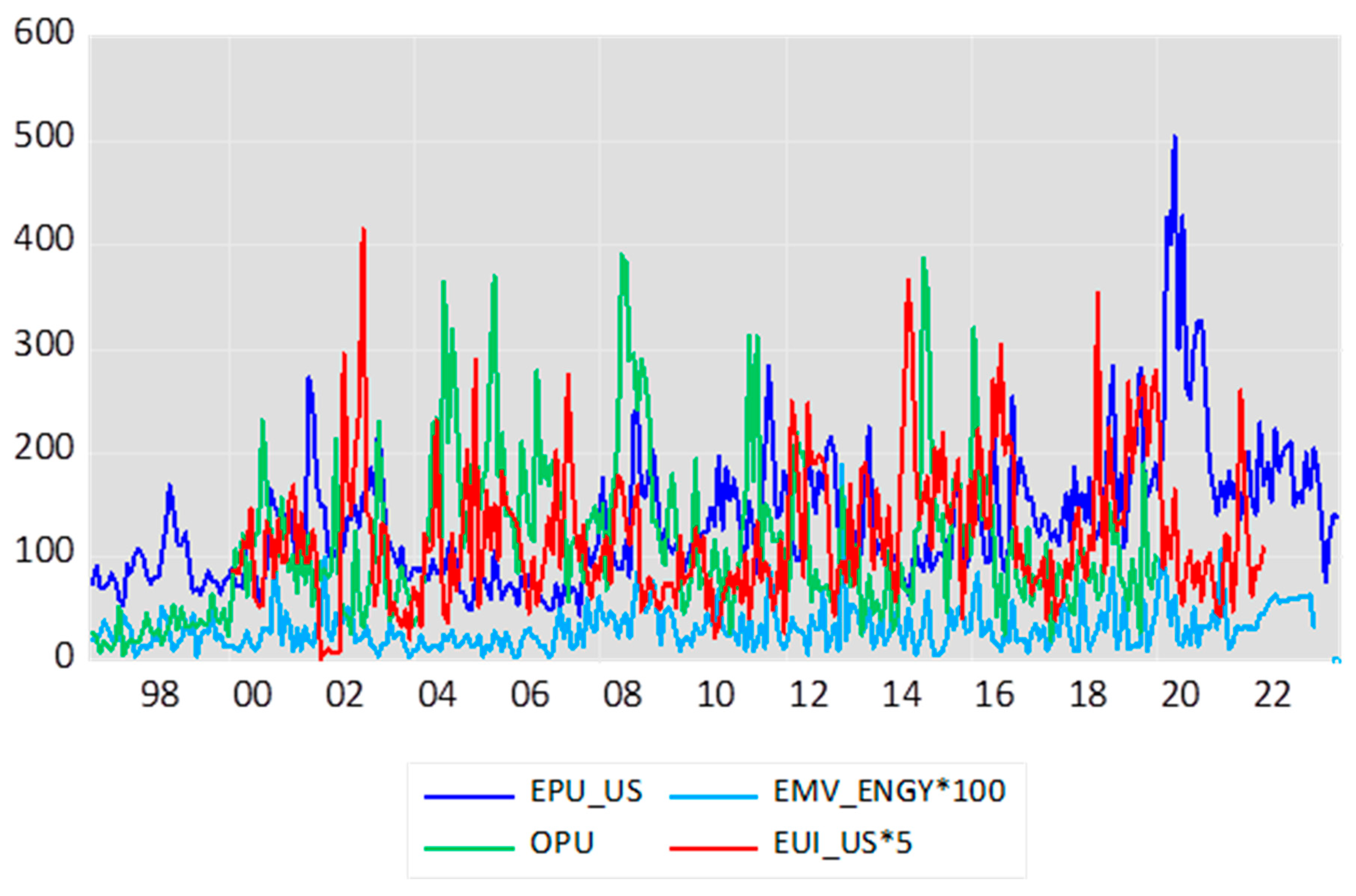
Table 1.
Summary statistics of stock returns across different sectors in the US market.
| Sector | Mean | Median | Maximum | Minimum | Std. Dev. | Skewness | Kurtosis | Jarque-Bera |
| ENGY | 0.629 | 0.688 | 28.513 | -45.502 | 6.914 | -0.760 | 9.491 | 598.2 |
| BMAT | 0.660 | 0.694 | 20.389 | -28.825 | 6.551 | -0.567 | 5.136 | 78.7 |
| CDIS | 0.787 | 1.091 | 16.608 | -17.291 | 4.908 | -0.318 | 4.252 | 26.6 |
| CSTP | 0.683 | 1.003 | 12.787 | -13.428 | 3.818 | -0.531 | 4.291 | 37.6 |
| FINA | 0.596 | 1.336 | 16.954 | -24.055 | 5.883 | -0.965 | 6.230 | 190.5 |
| HLTH | 0.773 | 1.280 | 12.821 | -13.022 | 4.079 | -0.533 | 3.573 | 19.7 |
| INDU | 0.774 | 1.261 | 15.931 | -22.608 | 5.543 | -0.567 | 4.608 | 52.1 |
| RLES | 0.668 | 1.334 | 27.404 | -36.352 | 5.967 | -1.190 | 9.920 | 720.7 |
| TECH | 0.894 | 1.535 | 19.533 | -32.333 | 7.407 | -0.676 | 4.555 | 57.1 |
| TELE | 0.398 | 1.045 | 27.492 | -17.171 | 5.650 | -0.177 | 4.714 | 41.2 |
| UTLI | 0.636 | 1.301 | 13.365 | -13.650 | 4.479 | -0.590 | 3.650 | 24.4 |
Notes: this table presents the descriptive statistics for each sectoral return, comprising monthly data from February 1997 to December 2022 (323 observations). Sectoral returns data includes Energy & Oil (ENGY), Basic Materials (BMAT), Consumer Discretionary (CDIS), Consumer Staples (CSTP), Financials (FINA), Health Care (HLTH), Industrials (INDU), Real Estate (RLES), Technology (TECH), Telecommunications (TELE), and Utilities (UTLI).
Table 2.
Correlations for sectoral returns in the US market.
| (1) | (2) | (3) | (4) | (5) | (6) | (7) | (8) | (9) | (10) | (11) | |
| (1) R_ENGY | 1 | ||||||||||
| ----- | |||||||||||
| (2) R_BMAT | 0.68 | 1 | |||||||||
| 16.61 | ----- | ||||||||||
| (3) R_CDIS | 0.50 | 0.74 | 1 | ||||||||
| 10.40 | 19.46 | ----- | |||||||||
| (4) R_CSTP | 0.43 | 0.56 | 0.64 | 1 | |||||||
| 8.55 | 12.06 | 14.90 | ----- | ||||||||
| (5) R_FINA | 0.58 | 0.72 | 0.79 | 0.64 | 1 | ||||||
| 12.77 | 18.78 | 23.47 | 14.97 | ----- | |||||||
| (6) R_HLTH | 0.42 | 0.56 | 0.67 | 0.76 | 0.67 | 1 | |||||
| 8.20 | 12.25 | 16.25 | 20.97 | 16.01 | ----- | ||||||
| (7) R_INDU | 0.62 | 0.81 | 0.85 | 0.59 | 0.82 | 0.65 | 1 | ||||
| 14.29 | 24.47 | 28.51 | 13.22 | 25.64 | 15.37 | ----- | |||||
| (8) R_RLES | 0.43 | 0.62 | 0.64 | 0.55 | 0.72 | 0.54 | 0.65 | 1 | |||
| 8.41 | 14.11 | 14.98 | 11.73 | 18.60 | 11.45 | 15.16 | ----- | ||||
| (9) R_TECH | 0.39 | 0.57 | 0.74 | 0.33 | 0.56 | 0.46 | 0.75 | 0.41 | 1 | ||
| 7.59 | 12.34 | 19.60 | 6.18 | 12.16 | 9.30 | 20.04 | 8.05 | ----- | |||
| (10) R_TELE | 0.37 | 0.48 | 0.60 | 0.47 | 0.51 | 0.46 | 0.60 | 0.36 | 0.58 | 1 | |
| 7.08 | 9.83 | 13.40 | 9.43 | 10.66 | 9.37 | 13.29 | 6.95 | 12.67 | ----- | ||
| (11) R_UTLI | 0.44 | 0.43 | 0.39 | 0.53 | 0.43 | 0.46 | 0.46 | 0.52 | 0.27 | 0.35 | 1 |
| 8.85 | 8.49 | 7.63 | 11.08 | 8.62 | 9.21 | 9.16 | 10.99 | 5.07 | 6.72 | ----- |
Notes: sectoral returns data includes Energy & Oil (R_ENGY), Basic Materials (R_BMAT), Consumer Discretionary (R_CDIS), Consumer Staples (R_CSTP), Financials (R_FINA), Health Care (R_HLTH), Industrials (R_INDU), Real Estate (R_RLES), Technology (R_TECH), Telecommunications (R_TELE), and Utilities (R_UTLI). For each variable, the first row reports the estimated correlation coefficients, the second row contains the estimated t-statistics.
Table 3.
Correlations for various measures of uncertainty.
| EPU | EMVE | OPU | EUI | CPU | |
| EPU | 1 | ||||
| ----- | |||||
| EMVE | 0.314 | 1 | |||
| 5.10 | ----- | ||||
| OPU | -0.138 | 0.114 | 1 | ||
| -2.15 | 1.77 | ----- | |||
| EUI | 0.104 | -0.057 | -0.036 | 1 | |
| 1.61 | -0.88 | -0.56 | ----- | ||
| CPU | 0.501 | 0.122 | -0.090 | 0.123 | 1 |
| 8.93 | 1.89 | -1.40 | 1.92 | ----- |
Notes: uncertainty variables include Economic policy uncertainty (EPU), Energy policy regulation induced stock market volatility (EMVE), Oil price uncertainty (OPU), energy uncertainty index and climate policy uncertainty (CPU). For each variable, the first row reports the estimated correlation coefficients, the second row contains the estimated t-statistics.
Table 4.
Estimates of US sectoral stock returns in response to EPU, EMV, OPU and EUI.
| Sector | C | ||||||||||
| ENGY | 5.090 | -0.017 | -1.082 | -0.010 | -0.027 | -0.377 | 23.055 | 0.218 | 0.903 | 0.04 | |
| 10.96 | -6.19 | -13.87 | -6.66 | -4.16 | -3.51 | 0.29 | 0.17 | 3.42 | |||
| BMAT | 5.584 | -0.018 | -0.712 | -0.016 | -0.022 | -4.132 | 23.457 | 0.610 | 0.654 | 0.07 | |
| 11.50 | -5.73 | -2.15 | -8.58 | -3.09 | -13.30 | 0.57 | 0.71 | 1.52 | |||
| CDIS | 2.691 | -0.003 | -0.520 | -0.006 | -0.026 | -7.342 | 8.657 | 0.635 | 0.803 | 0.00 | |
| 13.58 | -1.53 | -2.16 | -11.23 | -4.11 | -33.11 | 0.35 | 0.58 | 2.10 | |||
| CSTP | 2.276 | -0.004 | -0.215 | -0.001 | -0.027 | -2.930 | 7.667 | 0.233 | 0.889 | 0.04 | |
| 21.38 | -4.28 | -1.67 | -1.70 | -43.20 | -10.54 | 0.14 | 0.27 | 1.33 | |||
| FINA | 4.466 | -0.009 | -2.106 | -0.012 | -0.021 | -0.717 | 19.501 | 1.780 | 0.794 | 0.06 | |
| 12.37 | -4.19 | -4.42 | -7.62 | -2.79 | -1.14 | 0.41 | 0.59 | 2.70 | |||
| HLTH | 2.302 | -0.002 | -1.781 | -0.003 | -0.007 | -1.354 | 9.019 | 0.216 | 0.774 | 0.03 | |
| 27.71 | -2.30 | -5.08 | -6.12 | -3.35 | -1.66 | 0.25 | 0.35 | 0.99 | |||
| INDU | 4.564 | -0.012 | -2.191 | -0.011 | -0.013 | -5.249 | 4.248 | 0.417 | 0.830 | 0.07 | |
| 12.03 | -5.79 | -6.02 | -6.75 | -7.88 | -2.45 | 0.46 | 0.84 | 3.84 | |||
| RLES | 4.351 | -0.005 | -3.675 | -0.003 | -0.044 | -0.165 | 3.817 | 0.231 | 0.790 | 0.03 | |
| 11.00 | -1.98 | -9.06 | -3.01 | -5.08 | -3.28 | 0.70 | 0.95 | 3.74 | |||
| TECH | 4.072 | -0.014 | -1.228 | -0.016 | 0.021 | -0.829 | 33.830 | 0.213 | 0.757 | 0.02 | |
| 8.46 | -5.93 | -2.63 | -11.42 | 3.00 | -0.70 | 0.32 | 0.34 | 1.06 | |||
| TELE | 0.652 | 0.000 | -3.094 | 0.000 | 0.024 | -1.253 | 15.891 | 1.328 | 0.797 | 0.00 | |
| 2.30 | -35.63 | -6.40 | 14.42 | 4.18 | -0.61 | 0.34 | 0.57 | 2.35 | |||
| UTIL | 2.174 | -0.005 | -0.295 | 0.004 | -0.037 | -3.781 | 32.909 | 4.474 | 0.857 | 0.05 | |
| 9.05 | -3.18 | -17.68 | 5.22 | -7.68 | -8.41 | 0.22 | 0.49 | 2.90 | |||
Notes: the dependent variable is stock return ( Independent variables are: Economic policy uncertainty (EPU), Energy policy regulation induced stock market volatility (EMVE), Oil price uncertainty (OPU), energy uncertainty index (EUI). Sectoral data includes Energy & Oil (ENGY), Basic Materials (BMAT), Consumer Discretionary (CDIS), Consumer Staples (CSTP), Financials (FINA), Health Care (HLTH), Industrials (INDU), Real Estate (RLES), Technology (TECH), Telecommunications (TELE), and Utilities (UTLI). For each model, the first row reports the estimated coefficients, the second row contains the estimated z-statistics. The critical values of z-distribution at the 1%, 5%, and 10% levels of significance are 2.58, 1.96, and 1.65, respectively. is the adjusted R-squared for the coefficient of determination.
Table 5.
Estimates of US sectoral real stock returns in response to EPU, EMV, OPU and EUI.
| Sector | C | |||||||||
| ENGY | 4.916 | -0.017 | -0.994 | -0.010 | -0.027 | -2.593 | 27.395 | 0.171 | 0.832 | 0.05 |
| 12.25 | -7.47 | -14.20 | -5.51 | -5.15 | -1.79 | 0.26 | 0.18 | 1.43 | ||
| BMAT | 5.456 | -0.018 | -0.645 | -0.016 | -0.018 | -4.321 | 29.683 | 1.004 | 0.656 | 0.07 |
| 14.10 | -7.67 | -9.28 | -10.67 | -5.96 | -1.76 | 0.48 | 0.67 | 1.38 | ||
| CDIS | 2.499 | -0.003 | -0.564 | -0.006 | -0.025 | -7.345 | 11.841 | 0.220 | 0.921 | 0.00 |
| 14.86 | -1.71 | -2.13 | -7.99 | -4.01 | -21.52 | 0.20 | 0.32 | 2.84 | ||
| CSTP | 2.089 | -0.004 | -0.250 | -0.001 | -0.028 | -2.905 | 6.889 | 0.334 | 0.857 | 0.04 |
| 55.96 | -15.95 | -2.38 | -1.98 | -11.95 | -7.44 | 0.19 | 0.34 | 1.48 | ||
| FINA | 4.283 | -0.009 | -2.064 | -0.011 | -0.020 | -0.877 | 15.697 | 1.087 | 0.706 | 0.06 |
| 12.97 | -3.91 | -3.81 | -6.96 | -5.52 | -0.47 | 0.54 | 0.67 | 2.07 | ||
| HLTH | 4.395 | -0.012 | -2.206 | -0.010 | -0.013 | -5.212 | 5.321 | 0.494 | 0.778 | 0.07 |
| 11.27 | -4.45 | -4.10 | -6.10 | -5.34 | -2.36 | 0.52 | 0.92 | 3.13 | ||
| INDU | 4.142 | -0.005 | -3.700 | -0.003 | -0.046 | -0.113 | 4.952 | 0.304 | 0.786 | 0.03 |
| 17.95 | -3.64 | -7.54 | -7.88 | -6.48 | -6.65 | 0.62 | 0.86 | 3.29 | ||
| RLES | 3.930 | -0.013 | -1.185 | -0.016 | 0.022 | -0.301 | 7.872 | 0.698 | 0.822 | 0.02 |
| 8.46 | -4.87 | -1.88 | -9.25 | 2.58 | -1.49 | 0.42 | 0.69 | 3.55 | ||
| TECH | 0.542 | -0.001 | -4.049 | 0.004 | 0.018 | -1.094 | 7.654 | 0.875 | 0.751 | 0.01 |
| 7.38 | -3.09 | -59.94 | 15.27 | 11.10 | -2.59 | 0.42 | 0.75 | 2.51 | ||
| TELE | 1.982 | -0.005 | -0.391 | 0.004 | -0.038 | -3.485 | 11.633 | 0.774 | 0.858 | 0.05 |
| 8.81 | -3.14 | -9.67 | 4.07 | -8.63 | -4.42 | 0.30 | 0.49 | 2.77 | ||
| UTIL | 4.916 | -0.017 | -0.994 | -0.010 | -0.027 | -2.593 | 27.395 | 0.171 | 0.832 | 0.05 |
| 12.25 | -7.47 | -14.20 | -5.51 | -5.15 | -1.79 | 0.26 | 0.18 | 1.43 |
Notes: the dependent variable is real stock return (- Independent variables are: Economic policy uncertainty (EPU), Energy policy regulation induced stock market volatility (EMVE), Oil price uncertainty (OPU), energy uncertainty index (EUI). Sectoral data includes Energy & Oil (ENGY), Basic Materials (BMAT), Consumer Discretionary (CDIS), Consumer Staples (CSTP), Financials (FINA), Health Care (HLTH), Industrials (INDU), Real Estate (RLES), Technology (TECH), Telecommunications (TELE), and Utilities (UTLI). For each model, the first row reports the estimated coefficients, the second row contains the estimated z-statistics. The critical values of z-distribution at the 1%, 5%, and 10% levels of significance are 2.58, 1.96, and 1.65, respectively. is the adjusted R-squared for the coefficient of determination.
Table 6.
Estimates of US sectoral excess stock returns in response to EPU, EMV, OPU and EUI.
| Sector | C | |||||||||
| ENGY | 5.317 | -0.017 | -1.559 | -0.010 | -0.025 | -0.370 | 21.865 | 0.207 | 0.908 | 0.05 |
| 17.55 | -6.94 | -3.27 | -5.82 | -3.76 | -3.88 | 0.33 | 0.16 | 3.77 | ||
| BMAT | 6.617 | -0.020 | -1.583 | -0.016 | -0.025 | -4.207 | 38.912 | 0.873 | 0.476 | 0.09 |
| 14.31 | -6.74 | -3.92 | -9.49 | -3.20 | -6.02 | 0.65 | 0.71 | 0.83 | ||
| CDIS | 3.491 | -0.005 | -1.502 | -0.006 | -0.032 | -6.936 | 10.878 | 0.312 | 0.682 | 0.03 |
| 29.87 | -2.67 | -4.32 | -5.77 | -4.63 | -10.00 | 0.39 | 0.54 | 1.00 | ||
| CSTP | 2.818 | -0.006 | -0.335 | -0.002 | -0.031 | -2.590 | 6.484 | 0.173 | 0.832 | 0.06 |
| 8.46 | -2.97 | -2.81 | -2.39 | -9.17 | -13.64 | 0.31 | 0.24 | 1.65 | ||
| FINA | 4.305 | -0.008 | -2.742 | -0.011 | -0.017 | -0.855 | 13.373 | 0.812 | 0.697 | 0.07 |
| 10.61 | -3.17 | -5.18 | -7.56 | -3.04 | -2.17 | 0.58 | 0.66 | 1.87 | ||
| HLTH | 2.696 | -0.010 | -0.005 | -1.858 | -0.007 | 0.010 | 8.374 | 0.354 | 0.782 | 0.02 |
| 9.90 | -6.17 | -4.25 | -4.92 | -2.77 | 11.69 | 0.42 | 0.41 | 1.74 | ||
| INDU | 4.675 | -0.010 | -2.660 | -0.010 | -0.022 | -5.605 | 6.070 | 0.516 | 0.741 | 0.08 |
| 17.46 | -4.09 | -5.76 | -23.91 | -5.25 | -25.04 | 0.54 | 0.85 | 2.50 | ||
| RLES | 4.371 | -0.005 | -4.051 | -0.003 | -0.044 | 2.846 | 8.546 | 0.671 | 0.815 | 0.02 |
| 117.91 | -9.88 | -43.02 | -26.97 | -18.75 | 24.14 | 0.45 | 0.73 | 3.28 | ||
| TECH | 4.000 | -0.015 | -2.124 | -0.013 | 0.007 | -2.103 | 15.845 | 1.004 | 0.644 | 0.04 |
| 8.43 | -4.27 | -4.85 | -6.46 | 4.77 | -1.07 | 0.51 | 0.65 | 1.46 | ||
| TELE | 1.452 | -0.001 | -3.150 | -0.003 | 0.011 | -1.349 | 23.088 | 1.341 | 0.799 | 0.01 |
| 5.39 | -5.61 | -8.25 | -2.06 | 3.57 | -0.67 | 0.30 | 0.50 | 1.83 | ||
| UTIL | 1.592 | -0.004 | -0.300 | 0.004 | -0.025 | -2.230 | 14.952 | 1.067 | 0.793 | 0.03 |
| 18.81 | -4.23 | -1.39 | 5.36 | -8.79 | -1.98 | 0.31 | 0.50 | 1.77 |
Notes: the dependent variable is excess stock return (- Independent variables are: Economic policy uncertainty (EPU), Energy policy regulation induced stock market volatility (EMVE), Oil price uncertainty (OPU), energy uncertainty index (EUI). Sectoral data includes Energy & Oil (ENGY), Basic Materials (BMAT), Consumer Discretionary (CDIS), Consumer Staples (CSTP), Financials (FINA), Health Care (HLTH), Industrials (INDU), Real Estate (RLES), Technology (TECH), Telecommunications (TELE), and Utilities (UTLI). For each model, the first row reports the estimated coefficients, the second row contains the estimated z-statistics. The critical values of z-distribution at the 1%, 5%, and 10% levels of significance are 2.58, 1.96, and 1.65, respectively. is the adjusted R-squared for the coefficient of determination.
Table 7.
Estimates of US sectoral stock returns respond to various measures of uncertainties and crude oil price changes.
Table 7.
Estimates of US sectoral stock returns respond to various measures of uncertainties and crude oil price changes.
| Sector | C | Dumt | ||||||||||
| ENGY | 2.042 | -0.006 | -1.386 | -0.001 | -0.010 | 0.325 | -3.676 | 15.847 | 0.232 | 0.885 | 0.31 | |
| 7.66 | -2.97 | -3.10 | -3.48 | -11.65 | 35.96 | -2.39 | 0.17 | 0.29 | 1.71 | |||
| BMAT | 3.740 | -0.012 | -0.581 | -0.011 | -0.011 | 0.233 | -8.487 | 15.271 | 0.710 | 0.729 | 0.11 | |
| 32.98 | -8.19 | -2.39 | -9.02 | -2.36 | 16.65 | -8.34 | 0.48 | 0.68 | 1.95 | |||
| CDIS | 2.239 | 0.000 | -0.662 | -0.006 | -0.010 | 0.059 | -6.048 | 10.708 | 0.266 | 0.905 | 0.01 | |
| 28.38 | -5.96 | -2.28 | -19.68 | -6.25 | 18.51 | -27.90 | 0.20 | 0.34 | 2.32 | |||
| CSTP | 1.981 | -0.003 | -0.278 | 0.000 | -0.026 | 0.023 | -2.490 | 7.595 | 0.227 | 0.894 | 0.04 | |
| 13.32 | -2.00 | -2.64 | 6.47 | -10.67 | 3.42 | -4.04 | 0.11 | 0.26 | 1.15 | |||
| FINA | 4.157 | -0.008 | -2.089 | -0.011 | -0.018 | 0.035 | 2.647 | 12.737 | 0.713 | 0.730 | 0.01 | |
| 11.87 | -3.03 | -3.95 | -6.21 | -2.53 | 3.39 | 4.79 | 0.55 | 0.66 | 2.11 | |||
| HLTH | 2.116 | -0.002 | -1.784 | -0.003 | -0.007 | 0.018 | -1.833 | 9.766 | 0.306 | 0.897 | 0.03 | |
| 15.77 | -6.79 | -24.86 | -7.28 | -3.73 | 6.32 | -3.11 | 0.22 | 0.30 | 2.56 | |||
| INDU | 3.528 | -0.008 | -2.243 | -0.008 | -0.008 | 0.106 | -3.386 | 8.301 | 0.997 | 0.686 | 0.11 | |
| 14.66 | -3.91 | -4.34 | -26.50 | -11.69 | 16.85 | -1.33 | 0.48 | 0.87 | 1.97 | |||
| RLES | 4.235 | -0.005 | -3.768 | -0.004 | -0.044 | 0.005 | 0.146 | 12.196 | 0.680 | 0.812 | 0.03 | |
| 57.80 | -5.17 | -15.16 | -5.37 | -21.06 | 1.45 | 0.70 | 0.44 | 0.65 | 2.82 | |||
| TECH | 2.505 | -0.009 | -1.567 | -0.012 | 0.027 | 0.137 | -1.303 | 10.818 | 1.177 | 0.690 | 0.06 | |
| 6.40 | -2.94 | -2.10 | -6.28 | 4.28 | 18.19 | -0.67 | 0.44 | 0.80 | 2.05 | |||
| TELE | 0.241 | 0.001 | -2.405 | -0.001 | 0.025 | 0.032 | -1.625 | 17.915 | 1.460 | 0.754 | 0.00 | |
| 0.83 | 1.53 | -7.44 | -1.67 | 7.22 | 11.70 | -9.23 | 0.35 | 0.58 | 1.92 | |||
| UTIL | 1.868 | -0.004 | -0.379 | 0.005 | -0.036 | 0.029 | -2.985 | 10.019 | 1.207 | 0.800 | 0.05 | |
| 10.85 | -4.90 | -2.90 | 4.97 | -10.26 | 4.84 | -6.69 | 0.34 | 0.58 | 2.35 | |||
Notes: the dependent variable is stock return for sector i ( Independent variables are: Economic policy uncertainty (EPU), Energy policy regulation induced stock market volatility (EMVE), Oil price uncertainty (OPU), energy uncertainty index (EUI) and change of West Texas Intermediate (WTI) oil price in natural logarithm (. Independent variables are: Economic policy uncertainty (EPU), Energy policy regulation induced stock market volatility (EMV), Oil price uncertainty (OPU), energy uncertainty index (EUI) and changes in WTI oil price, . Sector i refers to Energy & Oil (ENGY), Basic Materials (BMAT), Consumer Discretionary (CDIS), Consumer Staples (CSTP), Financials (FINA), Health Care (HLTH), Industrials (INDU), Real Estate (RLES), Technology (TECH), Telecommunications (TELE), and Utilities (UTLI). For each model, the first row reports the estimated coefficients, the second row contains the estimated z-statistics. A similar result is achieved by using the Blent crude oil price change, . The critical values of z-distribution at the 1%, 5%, and 10% levels of significance are 2.58, 1.96, and 1.65, respectively. is the adjusted R-squared for the coefficient of determination.
Table 9.
Estimates of US sectoral stock returns respond to various measures of uncertainties and gasoline price changes.
Table 9.
Estimates of US sectoral stock returns respond to various measures of uncertainties and gasoline price changes.
| Sector | C | |||||||||||
| ENGY | 1.775 | -0.003 | -2.135 | 0.004 | -0.019 | 0.351 | -0.847 | -0.018 | 42.687 | 17.506 | 0.912 | 0.38 |
| 10.51 | -3.16 | -5.95 | 2.92 | -8.08 | 59.10 | -5.19 | -9.29 | 0.14 | 0.30 | 2.72 | ||
| BMAT | 3.199 | -0.029 | -1.342 | -0.007 | -0.005 | 0.175 | -1.791 | 0.004 | 16.311 | 0.699 | 0.698 | 0.17 |
| 11.01 | -7.63 | -2.32 | -8.61 | -0.62 | 21.35 | -10.75 | 0.55 | 0.51 | 0.73 | 1.83 | ||
| CDIS | 2.497 | -0.004 | -1.771 | -0.004 | -0.015 | 0.077 | -0.952 | 0.073 | 61.107 | 2.973 | 0.099 | 0.06 |
| 14.72 | -2.27 | -7.73 | -4.95 | -4.32 | 13.72 | -10.40 | 6.17 | 1.85 | 1.11 | 0.84 | ||
| CSTP | 2.077 | -0.001 | -1.186 | 0.001 | -0.024 | 0.059 | -0.721 | -0.014 | 7.842 | 0.181 | 0.923 | 0.05 |
| 12.70 | -3.10 | -3.07 | 1.53 | -6.14 | 14.16 | -6.97 | -1.90 | 0.08 | 0.25 | 1.25 | ||
| FINA | 4.285 | -0.014 | -3.212 | -0.009 | -0.014 | 0.074 | -1.619 | -0.010 | 10.439 | 0.996 | 0.670 | 0.12 |
| 26.56 | -5.87 | -5.77 | -13.78 | -12.68 | 11.22 | -12.07 | -1.04 | 0.56 | 0.93 | 2.17 | ||
| HLTH | 2.402 | -0.007 | -2.290 | -0.002 | -0.004 | 0.034 | -0.929 | 0.024 | 9.967 | 0.271 | 0.800 | 0.05 |
| 14.48 | -5.07 | -8.19 | -2.06 | -1.17 | 4.57 | -6.34 | 1.37 | 0.24 | 0.34 | 1.12 | ||
| INDU | 3.418 | -0.009 | -2.721 | -0.006 | -0.005 | 0.135 | -1.532 | -0.007 | 12.076 | 1.294 | 0.672 | 0.16 |
| 18.99 | -5.62 | -5.43 | -4.39 | -3.58 | 15.65 | -15.25 | -3.57 | 0.49 | 0.91 | 1.89 | ||
| RLES | 4.285 | -0.014 | -3.212 | -0.009 | -0.014 | 0.074 | -1.619 | -0.010 | 10.439 | 0.996 | 0.670 | 0.12 |
| 26.56 | -5.87 | -5.77 | -13.78 | -12.68 | 11.22 | -12.07 | -1.04 | 0.56 | 0.93 | 2.17 | ||
| TECH | 1.644 | -0.013 | -2.091 | -0.010 | 0.045 | 0.153 | -0.254 | 0.059 | 4.615 | 0.451 | 0.745 | 0.08 |
| 3.50 | -3.39 | -2.86 | -3.51 | 3.52 | 7.47 | -1.38 | 1.86 | 0.64 | 1.00 | 3.37 | ||
| TELE | 1.489 | -0.006 | -1.784 | -0.002 | 0.021 | 0.056 | -1.331 | -0.001 | 14.321 | 0.518 | 0.656 | 0.03 |
| 5.00 | -2.42 | -2.89 | -2.32 | 2.30 | 3.96 | -5.36 | -0.08 | 0.57 | 0.65 | 1.45 | ||
| UTIL | 2.251 | -0.001 | -1.150 | 0.005 | -0.030 | 0.048 | -1.482 | -0.030 | 7.406 | 0.976 | 0.795 | 0.05 |
| 9.48 | -1.99 | -3.06 | 5.10 | -6.74 | 6.16 | -8.85 | -2.97 | 0.35 | 0.63 | 2.46 |
Notes: the dependent variable is stock return for sector i ( Independent variables are: change in climate policy uncertainty in natural logarithm (), energy policy regulation induced stock market volatility (EMVE,t), oil price uncertainty (), energy uncertainty index (), and changes in gasoline price ( controlling the equity market volatility calibrated to financial crises (EMVFC) and infectious disease (EMVID). Sector i refers to Energy & Oil (ENGY), Basic Materials (BMAT), Consumer Discretionary (CDIS), Consumer Staples (CSTP), Financials (FINA), Health Care (HLTH), Industrials (INDU), Real Estate (RLES), Technology (TECH), Telecommunications (TELE), and Utilities (UTLI). For each model, the first row reports the estimated coefficients, the second row contains the estimated z-statistics. The critical values of z-distribution at the 1%, 5%, and 10% levels of significance are 2.58, 1.96, and 1.65, respectively. The 0.000 denotes a very small number. is the adjusted R-squared for the coefficient of determination.
Table 10.
Estimates of US sectoral stock returns respond to var Table 10. Estimates of US sectoral stock returns respond to various measures.
Table 10.
Estimates of US sectoral stock returns respond to var Table 10. Estimates of US sectoral stock returns respond to various measures.
| Sector | C | D-2008 | D-2020 | ||||||||||||
| ENGY | 1.263 | -0.004 | -0.003 | -2.450 | 0.002 | -0.010 | 0.373 | -4.519 | -8.436 | 19.987 | 0.279 | 0.871 | 0.37 | ||
| 7.47 | -5.19 | -17.03 | -19.71 | 1.78 | -6.76 | 41.23 | -2.84 | -9.86 | 0.28 | 0.40 | 2.26 | ||||
| BMAT | 2.521 | -0.009 | -0.002 | -1.878 | -0.008 | -0.010 | 0.206 | -8.720 | -1.454 | 18.289 | 0.705 | 0.709 | 0.16 | ||
| 12.51 | -6.77 | -10.79 | -5.84 | -6.15 | -5.95 | 16.30 | -11.38 | -1.84 | 0.49 | 0.66 | 1.70 | ||||
| CDIS | 2.024 | -0.004 | -0.001 | -1.315 | -0.004 | -0.017 | 0.077 | -7.235 | -7.726 | 13.609 | 0.258 | 0.896 | 0.04 | ||
| 19.53 | -4.58 | -9.93 | -4.46 | -8.28 | -7.50 | 9.96 | -11.62 | -5.28 | 0.21 | 0.35 | 2.21 | ||||
| CSTP | 1.608 | -0.003 | -0.001 | -0.600 | 0.002 | -0.025 | 0.049 | -3.524 | -4.450 | 8.022 | 0.243 | 0.889 | 0.07 | ||
| 21.40 | -8.75 | -9.52 | -3.04 | 9.30 | -8.42 | 6.37 | -8.39 | -2.06 | 0.12 | 0.27 | 1.22 | ||||
| FINA | 3.103 | -0.013 | -0.001 | -2.487 | -0.009 | -0.021 | 0.080 | -0.654 | -9.316 | .440 | 0.824 | 0.691 | 0.11 | ||
| 11.82 | -7.73 | -2.70 | -5.23 | -5.15 | -3.87 | 7.65 | -0.32 | -6.66 | 0.59 | 0.78 | 2.03 | ||||
| HLTH | 1.883 | -0.007 | -0.001 | -2.209 | -0.002 | -0.005 | 0.041 | -2.331 | -0.850 | 10.037 | 0.222 | 0.913 | 0.05 | ||
| 23.19 | -5.87 | -8.23 | -11.51 | -5.23 | -2.08 | 9.82 | -14.88 | -3.32 | 0.22 | 0 .23 | 3.02 | ||||
| INDU | 2.455 | -0.012 | -0.001 | -2.821 | -0.006 | -0.005 | 0.142 | -4.888 | -7.223 | 10.452 | 0.705 | 0.716 | 0.15 | ||
| 17.72 | -8.52 | -11.82 | -5.66 | -6.86 | -7.56 | 12.08 | -2.06 | -8.02 | 0.50 | 0.70 | 1.92 | ||||
| RLES | 3.292 | -0.005 | 0.001 | -3.956 | -0.001 | -0.038 | 0.057 | -0.441 | -4.192 | 11.591 | 0.820 | 0.717 | 0.05 | ||
| 19.35 | -2.31 | 2.21 | -8.61 | -0.85 | -6.04 | 5.07 | -0.14 | -4.23 | 0.56 | 0.78 | 2.14 | ||||
| TECH | 1.708 | -0.017 | -0.001 | -1.773 | -0.010 | 0.035 | 0.143 | -3.865 | 2.198 | 11.127 | 1.061 | 0.708 | 0.06 | ||
| 6.07 | -7.39 | -7.93 | -3.30 | -5.38 | 4.49 | 9.06 | -4.91 | 0.77 | 0.49 | 0.84 | 2.25 | ||||
| TELE | 0.666 | -0.006 | -0.001 | -2.093 | -0.003 | 0.023 | 0.060 | -1.869 | -2.354 | 20.258 | 1.824 | 0.726 | 0.02 | ||
| 3.47 | -8.69 | -4.64 | -5.35 | -3.48 | 3.98 | 5.17 | -7.48 | -1.27 | 0.38 | 0.57 | 1.79 | ||||
| UTIL | 1.187 | -0.002 | -10.001 | -0.790 | 0.007 | -0.032 | 0.043 | -2.513 | -5.891 | 11.945 | 0.557 | 0.858 | 0.06 | ||
| 14.78 | -9.79 | -2.12 | -2.73 | 6.99 | -16.62 | 20.28 | -2.91 | -3.02 | 0.30 | 0.45 | 2.46 | ||||
Notes: the dependent variable is stock return for sector i ( Independent variables are: change in climate policy uncertainty in natural logarithm (), interacting term energy policy regulation induced stock market volatility (EMVE,t), oil price uncertainty (), energy uncertainty index (), and changes in oil price ( controlling the equity market volatility calibrated to financial crises (EMVFC) and infectious disease (EMVID). Sector i refers to Energy & Oil (ENGY), Basic Materials (BMAT), Consumer Discretionary (CDIS), Consumer Staples (CSTP), Financials (FINA), Health Care (HLTH), Industrials (INDU), Real Estate (RLES), Technology (TECH), Telecommunications (TELE), and Utilities (UTLI). For each model, the first row reports the estimated coefficients, the second row contains the estimated z-statistics. The critical values of z-distribution at the 1%, 5%, and 10% levels of significance are 2.58, 1.96, and 1.65, respectively. The 0.000 denotes a very small number. is the adjusted R-squared for the coefficient of determination.
Disclaimer/Publisher’s Note: The statements, opinions and data contained in all publications are solely those of the individual author(s) and contributor(s) and not of MDPI and/or the editor(s). MDPI and/or the editor(s) disclaim responsibility for any injury to people or property resulting from any ideas, methods, instructions or products referred to in the content. |
© 2025 by the authors. Licensee MDPI, Basel, Switzerland. This article is an open access article distributed under the terms and conditions of the Creative Commons Attribution (CC BY) license (http://creativecommons.org/licenses/by/4.0/).
Copyright: This open access article is published under a Creative Commons CC BY 4.0 license, which permit the free download, distribution, and reuse, provided that the author and preprint are cited in any reuse.


