
Submitted:
07 April 2025
Posted:
09 April 2025
You are already at the latest version
Abstract
External fields modify the confinement potential and electronic structure in a multiple quantum well system, affecting the light-matter interaction. Here, we present a theoretical study of the modulation of the nonlinear optical response simultaneously employing an intense non-resonant laser field and an electric field. Considering four occupied subbands, we focus on a GaAs/AlGaAs symmetric multiple quantum well system with five wells and six barriers. By solving the Schrödinger equation through the finite element method under the effective mass approximation, we determine the electronic structure and the nonlinear optical response using the density matrix formalism. The laser field dresses the confinement potential while the electric field breaks the inversion symmetry. The combined effect of both fields modifies the intersubband transition energies and the overlap of the wave functions. Our results demonstrate a dynamic and adjustable control of the nonlinear optical response, opening up the possibility of designing optoelectronic devices with tunable optical properties.
Keywords:
GaAs/AlGaAs symmetric multiple quantum well system
; intersubband transition energies
; electro-optical modulation
; nonlinear optical response
1. Introduction
The control of light propagation through semiconductor heterostructures with multiple quantum wells (MQWs) has become a subject of intense research over the past decade [1,2,3,4,5,6,7,8,9]. In MQW systems, the effective coupling between wells usually arises when the structural parameters of the quantum wells are carefully modified and cause discrete localized energy levels of each well to begin to interact strongly. This interaction leads to extended states that spread over several wells rather than isolated quantized levels [10]. The above can lead to changes in the band structure that significantly alter the interaction of light with matter, leading to notable non-linear phenomena reported in experiments, such as high-harmonic generation processes including non-linear optical rectification (NOR) [11], second harmonic generation (SHG) [12], and third harmonic generation (THG) [13], which play a crucial role in modulating the emission spectrum of incident light [14]. In contrast to bulk materials, electronic confinement in MQW systems can be tailored, leading to enhanced non-linearities [15,16]. Furthermore, in MQW systems, the possibility of engineering diverse configurations enables tunable nonlinear responses with potential applications in electro-optical modulators [17,18], far-infrared detectors [19], semiconductor optical amplifiers [20], and nonlinear processes such as four-wave mixing [21].
In recent years, two approaches for modifying the nonlinear optical (NLO) properties in semiconductor heterostructures have been studied: the non-resonant intense laser (nIL) field and the electric field [22,23,24,25,26,27]. The nIL field alters quantum confinement, whereas the electric field breaks the inversion symmetry, enabling precise control over the NLO behavior. Although modifying structural parameters–such as well and barrier widths–in MQW systems has successfully generated enhanced optical nonlinearities, practical applications often require fixed quantum well dimensions. To address this, external fields offer a compelling alternative: they enable tunable control of higher-order harmonic generation while preserving the system’s structural configuration. For example, in a combined theoretical and experimental study, Miller et al. [28] report the effects of electric fields—both parallel and perpendicular to the quantum well layers—on optical absorption in GaAs/AlGaAs quantum well structures. Their results demonstrate that an electric field, whether applied parallel or perpendicular to the quantum-well layers, induces significant changes in optical absorption. Kasapoglu et al. [29] study the linear and nonlinear optical properties in a confining potential modeled from the symmetric and asymmetric harmonic-Gaussian potential of double quantum wells under the effect of an applied magnetic field. Their results show that the structural parameters allow control of the coupling between the two wells of the system, and the asymmetry parameter induces changes in the system’s selection rules. In addition, introducing a magnetic field produces blue or red shifts in the optical properties of the system. Additionally, Ozturk et al. [30] have investigated the effects of a laser field and an electric field, applied in different directions, on the intersubband optical absorption in a graded As/GaAs quantum-well structure. Their results demonstrate that the intersubband transitions depend directly on the applied external fields. Subsequent studies have exploited various approaches to modify the NLO properties, including temperature and pressure effects [31,32,33,34], magnetic fields [35], and excitonic effects [36].
It is well known that the application of an electric field on a MQW system modifies the confinement potential experienced by the electrons in the system, which can lead to the breaking of the inversion symmetry and, consequently, to an adjustment of the intersubband transition (ISBT) energies and dipole moment matrix elements (DMMEs), which are fundamental factors in the non-linear optical response of the system [37,38,39,40,41]. For example, the experimental work by Park et al. [42] presented a tunable nonlinear response resulting from the electrical modulation of an intersubband polariton metasurface composed of MQW. Other experimental studies have reported an electro-optical modulation effect of light at low voltages and speeds on the order of MHz in lithium niobate metasurfaces [43], electro-optical modulation in ring resonators [44,45], and significant second-harmonic generation as a result of a linear electro-optical effect in atomically thin 2D materials [46].
However, the nIL field induces a dressing effect on the confinement profile of the MQW system, modifying the effective potential by reducing the depth of the wells and decreasing the height of the barriers. Consequently, particle confinement is altered, leading to a shift in energy levels without changing the original symmetry of the system [47]. Sakiroglu et al. [48] demonstrated the effect of the nIL field on the non-linear optical properties of a Morse quantum well. Their results reveal shifts in the positions of the peaks in both the optical absorption coefficient and the refractive index. Furthermore, other studies indicate that the combined effects of nIL and magnetic fields can modulate the interaction forces between particles and alter the energy level [49]. Many previous studies on the NLO response in multiple quantum well systems have focused on its electrical or optical modulation. However, electro-optical modulation has received limited attention, although it is known that effective coupling between wells in MQW structures can induce strong light-matter interactions, significantly enhancing the nonlinear response.
Due to the external fields playing a determining role in tailoring the system’s NLO response, achieving independent and simultaneous tuning of both fields is highly desirable. For this purpose, it is convenient to propose a GaAs/AlGaAs semiconductor heterostructure, because of the mature fabrication techniques that allow precise control over the composition and dimensions of the wells [50]. In addition, these heterostructures feature well-defined energy levels and a bandgap that can be tuned by external fields [51].
In this contribution, we perform flexible control over the ISBT energies and DMMEs by applying the nIL and the electric fields. To this end, we theoretically investigate the effect of external fields on the electronic properties of the MQW system through optical and electrical means [Figure 1a]. We focus on a As MQW system, considering four electron subbands. Our results demonstrate that combining these external fields enables a unified electro-optical manipulation of the NLO response. Furthermore, we show that the external fields have a measurable impact on the ISBT energies and DMMEs. Finally, we present optimal configurations of the external field values that modulate the transition-energy crossings, and the manipulation of the position of the resonant peaks involved in the susceptibility coefficient, which determines the light conversion efficiency and allows dynamic and adjustable control of the NLO response.
This paper is organized as follows. In Section 2, we present the derivation of the laser-dressed potential energy for a MQW system under the influence of the nIL field and derive the expressions for the coefficients of the NLO response and the DMMEs. Section 3 defines the parameters used in our study. Section 4 presents our main results on the influence and control of the NLO response through external fields. In Section 5, we summarize our main findings.
2. Theoretical Framework
First, we outline the dressing effect of the nILF field on the confining potential. Next, we detail the derivation of the NLO response using the nonlinear susceptibility coefficients. In addition, we provide the relevant expressions for the DMMEs. We consider a symmetric MQWs system with GaAs (As) well (barrier) regions of and widths, respectively. The total length (L) of the system is the sum of 6 barriers and 5 wells. We will calculate the corresponding subband energy levels, density probability, and NLO response, such as the NOR, SHG, and THG, derived from the intersubband transitions of the MQWs under a nIL field and an electric field.
2.1. Laser Dressed Potential Energy
The time-dependent Schrödinger equation in the effective-mass approximation, under the effect of an applied external electric field and a non-resonant intense laser field, the confinement potential V changes according to the Kramers-Henneberger transformation as follows [52]:
where is the position-dependent electron effective mass, e is the absolute value of electron charge, is the electric field, and is the laser-dressed potential of the system. The quantum wells are grown along the x-axis and the external electric field lies along the growth direction, and we assume that the nIL field is polarized in the same direction. The reference frame origin is set at the geometrical center of the heterostructure.
We use the separation of variables method to obtain a 1D differential equation for the x-coordinate. In this approach, the wave function is written in terms of the wave vector and the electron coordinate in the plane (perpendicular to the growth direction of the heterostructure) . Assuming the bottom of all energy subbands, then . Therefore, by applying a Fourier expansion to the potential and using Floquet’s theory [53], while considering only a high-frequency laser field, we obtain the time-independent Schrödinger equation as follows:
where is the electron energy eigenvalue associated with the eigenfunction of the n-th subband and F is the electric field strength. A shift of is introduced in the x-coordinate to set the zero of the potential energy at that point of the structure. The second term of Equation (2) accounts for the laser-dressed potential and is written as:
In the above equation, we have replaced the explicit form of the term associated with a classical displacement of the electron under the influence of an electric field . Where is the non-resonant frequency, indicate the propagation direction of the field and , being the field strength and the laser-dressing parameter [47].
The intensity of the nIL field is determined by the laser-dressing parameter , which can be defined in terms of the time-averaged intensity of the laser field as [20]:
where c is light speed and is the permittivity of the vacuum. Following a similar procedure to the one described in Ref [54]: (i) We choose a specific amplitude in the high-intensity regime of the laser field (i.e. the laser-dressing parameter) nm. (ii) For our GaAs/AlGaAs heterostructure, the characteristic intensity at high frequencies is defined by [55], where nm is the effective Bohr radius, THz is the laser frequency, and is the relative dielectric constant at high frequencies and k is the Coulomb constant. (iii) To deal with the problem of non-uniform effective masses, we use the average effective mass approximation [56]:
and represent the effective mass corresponding to GaAs wells and AlGaAs barriers. Thus, we obtain an approximate value of the characteristic intensity at high frequencies, which is W/. (iv) Using Equation (4) for nm, we calculate a maximum intensity value, . Although the maximum value of the intensity exceeds the characteristic intensity at high frequencies, usually intensities of about are accepted in experimental procedures [57,58,59].
Finally, we solve the differential equation corresponding to the Schrödinger equation [Equation (3)] using the finite element method (FEM) implemented in the COMSOL-Multiphysics semiconductor module [60]. After determining the energy levels and corresponding wave functions, we computed the NLO properties and the relative shifts in the ISBT energies and DMMEs.
2.2. Nonlinear Optical Response
To study the NLO response, we employ a semi-classical approach. This method combines a quantum description of the interacting particle with a classical representation of the radiation field. The radiation field is modeled as monochromatic optical radiation, characterized by the electric field , which is polarized along the growth direction of the quantum wells, i.e.
where is the complex amplitude. Using the density matrix formalism and assuming a phenomenological approach to the dissipative process, the Liouville–von Neumann equation explicitly describes its time evolution via the following master equation [61]:
where is the density matrix operator, is the dipole moment operator and are the matrix terms of the phenomenological operator . The steady-state density matrix is diagonal and its elements represent the electron populations of the i-th energy levels . is the free Hamiltonian of the system in the absence of the electric field for the four subbands, and is the perturbation term that accounts for the light-matter interaction. The phenomenological operator incorporates damping effects caused by interactions between electrons and phonons and electron-electron collisions. We assume that is a diagonal matrix associated with the relaxation process and its elements are the inverse of the relaxation time that involves the |m⟩ state, with [62,63]. To simplify, we use the notation for the term .
The master equation [Equation (7)] is solved using a perturbative method, in which the system is divided into an unperturbed part and a perturbative part that introduces slight corrections to the system dynamics. This approach yields a series solution, each perturbative order adding corrections to the total evolution. Consequently, the density matrix is expanded perturbatively in terms of the electric field as:
Replacing into the Equation (7) and using the completeness relation , we have:
Here is the Kronecker delta (0 for and 1 for ). We can expand the different perturbative orders of as follows:
We assume, in the weak probe approximation, all electron population at is in the ground state, which requires that , and for . The analytical solution for the matrix elements at different perturbative orders is obtained using a procedure similar to that described in Refs. [61,62].
The electronic polarization and susceptibility coefficients are related through the light polarization degree, induced by the electric field . This relation is derived by equating terms proportional to in the polarization expansion with those obtained from the perturbative expansion of the density matrix in the steady-state response with , through the following equation [64]:
where V is the volume of the system, , , , and are the linear optical susceptibility, nonlinear optical rectification, second harmonic generation, third order linear susceptibility and third harmonic generation, respectively. This work focuses on the coefficients associated with optical rectification, second harmonic generation, and third harmonic generation.
Finally, we find the corresponding expressions per unit surface as follows:
where is the intersubband transition energy, and is the carrier density. In the above equations, the DMMEs are defined as:
where , () are the off-diagonal (on-diagonal) DMMEs, respectively. The eigenfunctions and are obtained from Equation (2).
3. System and Parameters
The system consists of a sequence of five coupled GaAs quantum wells and six As barriers, as illustrated in Figure 1b. Because of the small separation between subbands, close to optical phonon energies ( meV in GaAs), this structure exhibits short excited states lifetimes ( ps) [65]. This short lifetime of electrons in the excited subbands primarily arises from electron-phonon interactions, the dominant mechanism for energy relaxation in this system.
For the calculations, the following parameters have been used from experimental results: an Al concentration of , based on the distribution rule for the band offset between the conduction and valence bands, respectively. The barrier height is expressed as meV, where [66]. We consider well (barrier) width of 4 nm (3 nm). The effective electron mass for GaAs (AlGaAs) is (), , , , and [13,64,67,68].
4. Results and Discussion
In this section, we discuss the external field-mediated electro-optical control of the ISBT and DMMEs. To proceed systematically, we first analyze the influence of individual fields (electric and nIL) separately, followed by their combined effect. Next, we discuss cases where ISBT and wavefunction overlap are manipulated using purely electrical or optical means. Finally, we delve into the impact of simultaneous electric and laser fields on the NLO response of the MQWs system.
4.1. Influence of the External Fields on the DMMEs and the ISBT
Figure 1b shows the profile of the conduction band for a As symmetric MQW system composed of five wells and six barriers. The probability density associated with the first four states is also depicted, corresponding to eigenenergies to . Without any external field ( and ), the initial symmetric confinement potential profile results in alternating symmetric and antisymmetric parity for the wave functions. The electrons in the ground state are located to a greater extent at the central quantum well center (see blue curve), with the probability density being maximum at this point and different from zero in all the wells, which indicates that there may be tunneling of the electrons. The maximum probability density localizes in the central well due to the electrons favoring regions of minimal confinement, in agreement with theoretical expectations.
Figure 2 shows the modifications to the potential due to the presence of the nIL field and the electric field. Figure 2a shows the potential modified by a nIL field without an electric field (, black line) and the first four probability densities of the confined states. Under the presence of the nIL field, a new symmetric potential arises in the system of wells and barriers, which directly depends on the changes in the laser-dressing parameter , as shown in the figure (compare Figure 1b with Figure 2a). For nm, the number of wells is modified in the system, going from five to four effective wells; note that in the initial system, at the center position (), there was one well and the laser effect transforms this well into a barrier. Additionally, all wells become shallower and wider at the top and narrower at the bottom, leading to a noticeable separation in the energy levels. This behavior has also been previously reported by Lima et al. [69] for values of the laser parameter larger than the well width . As a result, the electrons are distributed mainly in the two central wells (see blue curve).
Figure 2b shows the potential profile modified by the effects of the electric field without the nIL field () and its corresponding probability densities. The electric field induces polarization in the system, tilts the potential, and shifts the charge distribution, breaking the inversion symmetry of the system. Due to this, the electrons experience a force that displaces them parallel to the fields and locates them in the wells on the left. Figure 2c shows the potential under the presence of both fields, the nIL ( nm) and the electric field ( kV/cm). We observe a combined effect in the modified potential: alterations in the shapes of the wells and barriers caused by the nIL field, and a tilt induced by the electric field. Note that, with the action of both fields, the MQW system undergoes a significant change in the electron confinement, which could alter its electronic and optical properties.
Figure 3a-d show the ISBT energies between the first four states as a function of the laser-dressing parameter and the electric field strength for the symmetric As MQW system illustrated in Figure 1. Note that the ISBT energies are scaled (i.e., divided by a factor of two and three , respectively), which is a direct consequence of the quantization of energy levels in confined semiconductor structures. This scaling facilitates the analysis of the optical properties discussed later in this investigation. In each panel, the curves include the first four states as functions of the aforementioned external fields, which allows for a direct observation of the ISBT energy modification induced. Figure 3a and Figure 3d show the ISBT energies as a function of the electric field. Without the nIL field [Figure 3 a], a monotonic increase in the behavior of the ISBT energies is observed with increasing electric field strength (see Table 1). Furthermore, three ISBT energy intersections occur: and , in the electric field range , kV/cm, these factors come from the denominators of the equations. () and () to obtain a maximum in the corresponding susceptibilities. The intersections result from the coincidence between ISBT energies in a specific range of electric field values. This coincidence influences the dynamics of the optical response of the system, as will be discussed later. The insets in all panels of Figure 3 show that the energies do not present crossings or anticrossings. In contrast to Figure 3a, in Figure 3c the and intersections are observed, in this case for an electric field value of kV/cm, instead of the kV/cm of panel (a). This shift towards higher energy values arises because of the modifications in the potential profile induced by the nIL field. Figure 3b shows the ISBT as a function of the laser-dressing parameter without an electric field. The increase in the laser-dressing parameter induces a monotonic increasing behavior of the ISBT energies without intersections between them. In contrast, the application of an electric field, Figure 3 d, is again responsible for the occurrence of intersections between ISBT energy pairs: and , for laser-dressing parameter values of nm.
Taking into account the effects of external fields on the ISBT energies, we can now explore the manipulation of the DMMEs through these fields. The DMMEs as a function of the electric field strength without a nIL field () and with a nIL field () are shown in Figure 4a and Figure 4c, respectively. In Figure 4a, without the nIL field, a monotonic decrease is observed in the matrix elements and as the strength of the electric field increases. For and , a non-zero value is obtained, due to the breaking of the symmetry inversion induced by the electric field, which enables transitions that were previously forbidden. With increasing electric field strength, the wave functions shift and deform, reaching at some point an optimal overlap (kV/cm) that maximizes the DMMEs and . For higher field values, distortion and excessive shifting reduce the overlap, causing the matrix elements to decrease again. In contrast, the DMMEs and shows a monotonic decrease as the electric field strength increases, suggesting a lower overlap of the wave functions. In Figure 4c, the nIL field causes the matrix elements and to decrease slightly as the electric field increases (compared to Figure 4a). For DMMEs involving the fourth state ( and ), a non-monotonic behavior is appreciable because this state, for high nIL field strengths ( nm), can be coupled to the continuum states (cyan line in Figure 2c). Furthermore, the maximum value of the matrix elements and shifts towards higher values of the electric field (kV/cm) and remains almost constant from that value onward. All this suggests that the presence of the nIL field alters the overlapping wave functions and shifts the values of the electric field where maxima occur in the DMMEs.
Figure 4b and Figure 4d show the DMMEs as a function of the laser-dressing parameter, without an electric field () and with an electric field ( kV/cm), respectively. In Figure 4b, with , a slight decrease of the matrix elements and is observed as the nIL field increases. Furthermore, and remain constant at zero (the associated lines are superimposed on the plot), indicating that the nIL field slightly alters the overlapping of the wave functions and does not break the inversion symmetry, preserving its initial selection rules. In Figure 4d, the electric field kV/cm breaks the inversion symmetry of the system and the DMMEs increase as a function of the laser-dressing parameter, reaching a maximum value for nm, and slightly decreasing from that value onwards. The reason behind this is the displacement and overlapping of the wave functions produced by the effects of both fields.
Before calculating the susceptibility coefficients, it is convenient to study how these external fields alter the NLO response in the system. These changes are, in principle, associated with the so-called geometric factors, which refer to the terms involving the product between the DMMEs in each susceptibility coefficient. Figure 5a and Figure 5b show the geometric factor , where , associated with the nonlinear optical rectification NOR [Equation ()], as a function of the electric field strength and the laser-dressing parameter, respectively. In Figure 5a, without the nIL field (solid line), it is observed that the geometric factor reaches its maximum value for an electric field of kV/cm, decreasing from that point onward as the field increases (see Table 2). With an nIL field of nm (dashed line), the maximum value shifts to higher field intensities and is reached for an electric field of kV/cm. The reason for this lies in the non-monotonic variation of the DMMEs and with the electric field, and their product reaches a maximum value in the ranges where both are relatively large (see Figure 4a). Figure 5b demonstrates that, in the absence of an electric field (solid line), the geometric factor remains zero when varying the laser-dressing parameter because the nIL field does not break the inversion symmetry of the system so that the term involving the matrix elements and is zero (see Figure 4b). In contrast, in the presence of an electric field (dashed line), a non-monotonic behavior is observed in the curve associated with the geometric factor, reaching its maximum value for a nIL field of nm.
Figure 6a and Figure 6b show the geometric factor , associated with second harmonic generation (SHG) [Equation ()], as a function of the electric field strength and the laser-dressing parameter, respectively. In Figure 6a, in the absence of the nIL field (solid line), it is observed that the geometric factor reaches its maximum value for an electric field of kV/cm. On the other hand, when applying an nIL field to the system (dashed line), a reduction is observed for the maximum values, in addition to a shift towards an electric field value of kV/cm. Figure 6b manifests that in the absence of an electric field, the geometric factor remains constant at zero by varying the laser-dressing parameter because the matrix element requires the inversion symmetry breaking induced by the electric field (see Figure 4b).
Figure 7a and Figure 7b show the geometric factor , associated with third harmonic generation (THG) [Equation (15)], as a function of the electric field strength and the laser-dressing parameter, respectively. In comparison to the geometric factors discussed above, this does not require the electric field-induced inversion symmetry breaking, due to the alternating symmetry and antisymmetric parity of the wavefunctions; therefore, the matrix elements involved are non-zero as a function of the external fields, as shown in Figure 4. In Figure 7a, the geometric factor exhibits a monotonic decreasing behavior as the intensity of the electric field increases, both in the absence of the nIL field (solid line) and in the presence of nIL field (dashed line). The main difference lies in the maximum values reached in kV/cm by this factor in the presence of the nIL field, while without this field, the maximum value is lower, with a more pronounced decrease as the electric field strength increases. Figure 7b shows the curves of the geometric factor as a function of the nIL field; in the absence of an electric field (solid line), this factor remains nearly constant for a laser-dressing parameter ranging from 0 to nm. For larger values of the laser-dressing parameter, the geometric factor decreases monotonically. When an electric field of kV/cm is applied, the opposite behavior is observed, i.e., the geometric factor monotonically increases for nm, being rather constant for lower values.
4.2. External Fields Control Nonlinear optical response
Figure 8 shows the NOR coefficient () as a function of the incident photon energy for different values of the electric field strength and the nIL field. Panel (a) of this figure shows that in the absence of the nIL field (), the peak associated with the NOR coefficient reaches its maximum value when kV/cm. As the electric field increases, this peak experiences a blueshift, and its maximum value decreases. The energy shift is due to the energy of the intersubband transition , involved in the NOR coefficient [Equation (12)], which exhibits a monotonic increasing behavior (black line in Figure 3a). The above indicates that the increase in the electric field generates a separation between the intersubband levels, shifting the resonance peak towards higher energies. Additionally, the decrease in the maximum value occurs because the electric field alters the shape and position of the quantum state wave functions, thereby modifying their overlap. This effect is illustrated by the solid line in Figure 5a, which shows that the geometric factor reaches a maximum value at approximately kV/cm before decreasing as the field increases. Finally, it is important to note that for , the NOR peak is zero since the electric field is required to generate the non-linear response of the system.
For comparison with panel (a), panel (b) of Figure 8 illustrates the NOR coefficient as a function of the incident photon energy for the same four electric field strength values, but in the presence of the nIL field ( nm). The first remark when looking at panels (a) and (b) is that the magnitude of the maximum value reached by the NOR coefficient in kV/cm is lower in the presence of the nIL field. Under this setup, a blueshift in the NOR peak and an increase in its maximum value for kV/cm; however, from that value, the maximum value decreases. The reason for this blueshift is that, under the influence of the nIL field, the geometric factor associated with the NOR (see Figure 5a, dashed line) experiences a shift in its maximum value and a decrease in its magnitude. Finally, Figure 8c presents the NOR peak as a function of the photon energy for different values of the laser-dressing parameter in the presence of an electric field of kV/cm. In contrast to Figure 8a and Figure 8b, here the blueshift of the peak is less pronounced, and its magnitude increases as grows. The nIL field-induced confinement produces a slight blueshift in the intersubband energy as increases (black line in Figure 3d), influencing, therefore, on the separation between levels, which turns into a less marked shift towards higher energies. As previously discussed, the curve associated with the geometric factor (Figure 5b, dashed line) determines the behavior of the NOR peak maximum value. The combined effect of the electric field and the nIL field offers a tunable mechanism that modifies both the energy level separation and the overlap of the wave functions. These variations dynamically tune the magnitude and spectral position of the nonlinear optical rectification.
Figure 9 shows the SHG coefficient () as a function of the incident photon energy for different values of the electric field and the nIL field. In Figure 9a, when (absence of nIL field), the SHG coefficient exhibits a blueshift with the photon energy, and when it reaches its maximum value ( kV/cm, pink curve) the magnitude decrease as the electric field intensity increases. This blueshift is due to the monotonic increasing behavior of the intersubband transition energies and with the electric field strength (see Figure 3a, black and red curves). Furthermore, we observe that at kV/cm, the two characteristic peaks of the SHG coefficient are merged into a single peak with the highest magnitude; however, as the electric field increases, these peaks move apart. This separation influences the maximum value of the SHG coefficient, which describes the efficiency of the process and depends on both the intersubband transition energies and the incident photon energy. In contrast to Figure 8, the maximum value of the SHG coefficient is not governed exclusively by the behavior of the geometric factor , but depends mainly on the approach or intersections between the ISBT energies. When the peaks move apart, the energies and become more distinguishable, indicating a change in the electronic structure of the multiple quantum well system induced by the electric field. This phenomenon is clearly shown from the variations in the level spacing (see Figure 3a, black and red curves): at kV/cm, the transition energies are close (even crossing at kV/cm, pink circle Figure 3a), as the electric field increases, they start to move apart. The moving apart of the peaks reduces the efficiency of SHG since the mismatch between resonances prevents the incident photon energy from being transferred efficiently, producing a notable decrease in the maximum coefficient value. Nevertheless, as the peaks move apart, SHG becomes more selective concerning the photon incident frequencies, implying that the system will respond strongly only at specific frequencies corresponding to the individual ISBT energies.
In Figure 9b, the presence of the nIL field ( nm) causes a blueshift and an increase in the magnitude of the SHG coefficient as the electric field strength increases, reaching its maximum value at kV/cm (pink curve), from this point on, the coefficient decreases. The blueshift is associated with an increase in the ISBT energies with the electric field strength (see Figure 3c). On the other hand, in contrast to Figure 9a, the two characteristic peaks of the SHG coefficient are initially separated and closer as the electric field strength increases. When an approach or intersection occurs between the intersubband transition energies and ( kV/cm, see Figure 3c pink circle), the two characteristic peaks of the SHG coefficient merge into a single, more intense peak. Physically, this indicates that the incident photon energy coincides, at some point, with the intersection between the ISBT energies, which maximizes the SHG efficiency under this resonance condition. In this scenario, the incident photon energy is transferred more effectively to the second harmonic generation process. The induced coincidence, through the two external fields, between the ISBT energies involved in the SHG leads to a significant increase in the magnitude of the second-harmonic signal. Finally, Figure 9c shows that under a fixed electric field of kV/cm, both a blueshift and an increase in the maximum value of the SHG coefficient occur as the laser-dressing parameter increases. Initially, the characteristic peaks of the SHG coefficient are separated. However, as the laser-dressing parameter increases, these peaks become closer. In this case, the ISBT energies and do not cross (see Figure 3d), but there is an approach between them as the nIL field increases; for that reason, we observe at nm the highest magnitude of the SHG coefficient.
Figure 10a and Figure 10b show the THG coefficient () as a function of the incident photon energy for different values of the electric field strength in the absence () and presence ( nm) of the nIL field, respectively. In Figure 10a, for electric field intensities ranging in kV/cm, the THG coefficient shows a blueshift together with a coalescence of the three characteristic peaks and increase in the magnitude. The coefficient for kV/cm breaks the previous trend, and undergoes a notable decrease in magnitude and a splitting of the peaks. The blueshift is due to the monotonic increase of the ISBT energies , , and (see Figure 3a). The coalescence and splitting of the three peaks is attributed to the fact that, in the range of kV/cm, these transition energies approach to each other considerably (even presenting intersections between pairs such as , and , but no coincidence between the three energies in a single point is found), whereas for kV/cm and remain close and separates, originating the appearance of two peaks close together and one further away. As previously discussed, the behavior of the geometrical factor as a function of F (see Figure 7a, dashed line) does not explain the maximum values reached by the THG coefficient, which are mainly related to the proximity and intersections between the ISBT energies. In particular, the maximum value observed of the THG coefficient at kV/cm indicates that for this specific electric field value, the ISBT energies , and are closer, which favors the efficiency of the THG process. Whereas for kV/cm, the separation of the peaks reduces the magnitude of the THG coefficient and confers selectivity concerning the incident photon frequencies. In comparison with Figure 10a, in Figure 10b the presence of the nIL field causes the characteristic THG peaks to be initially more separated, preserving the afore discussed blueshift but causing the occurrence of the maximum value at kV/cm. These results indicate that, by applying the nIL field, it is possible to adjust the electric field values at which approaches or intersections occur between ISBT energies and, in this way, determine the optimal combination of external fields that improves the THG efficiency. Indeed, these results demonstrate that the efficiency of the THG process can be improved when external fields induce coincidences between the ISBT energies. Moreover, external fields can also separate the ISBT energies and make the THG process highly selective with incident photon frequencies.
Figure 10c and Figure 10d show the THG coefficient as a function of the incident photon energy for different values of the laser-dressing parameter in the absence () and presence ( kV/cm) of the electric field, respectively. In Figure 10c, as the nIL field increases, a blueshift is observed in the THG coefficient, accompanied by a progressive separation of the three characteristic peaks and a decrease in their magnitude. This blueshift is attributed to the monotonic increase of the ISBT energies , and as a function of the nIL field (see Figure 3c). The separation of the peaks significantly influences the magnitude of the THG coefficient, suggesting that, in the multiple quantum well system, increasing the nIL field reduces the THG efficiency, although it improves the selectivity concerning the incident photon frequencies. This behavior could be useful in applications that require selective interaction with specific frequencies. On the other hand, Figure 10d shows that, in the presence of an electric field, the THG coefficient undergoes a weaker blueshift and its magnitude increases considerably as the nIL field increases. This small shift is due to the slight growth of the ISBT energies with the nIL field (see Figure 3d). For an electric field of kV/cm, the THG coefficient’s characteristic peaks align with the ISBT energies’ dependence on the laser-dressing parameter. We observe that and are very close, while is separated (see Figure 3d), resulting in two closely spaced peaks and one well-defined peak. This trend persists until the laser-dressing parameter reaches approximately nm. Beyond this value, an intersection occurs between the energies and , causing the two adjacent peaks to merge into a single peak. However, the peak corresponding to remains isolated. Notably, under these conditions, the magnitude of the THG coefficient increases substantially (see blue curve). A similar effect emerges at nm, where another intersection arises between and . All three ISBT energies converge at this point, leading to a higher enhancement in the magnitude of the THG coefficient.
5. Conclusions
In this research, we theoretically study the modulation of the non-linear optical response in a As symmetric multiple quantum well system under the simultaneous application of an IL field and an electric field. On the one hand, the nIL field modifies the electron confinement potential without altering the initial symmetry of the system; the so-induced changes affect the overlap of the wave functions and the electronic structure, leading to variations in the spacing between subbands and, consequently, in the ISBT energies. On the other hand, the electric field tilts the confinement potential. It alters the electronic distribution, breaking the inversion symmetry and enabling transitions between states previously forbidden by the selection rules. In addition, this field modifies, analogously to the nIL field, both the wave functions’ overlap and the separation between subbands.
To analyze the non-linear optical response, we determine the impact of each field on the ISBT energies and the wave function overlap, quantified by the geometrical factor. The results show that the simultaneous application of both external fields enables the manipulation of both the overlap of the wave functions and the coupling or intersection between the ISBT energies, which are determining factors in the nonlinear optical response of the system. The behavior of the geometrical factor as a function of the nIL field and the electric field determines the efficiency of the non-linear optical rectification; the system reaches a high efficiency when this factor reaches its maximum value. Additionally, accidental coincidence, induced by external fields, between pairs of ISBT energies improves the efficiency in the second and third harmonic generation. Instead, the ISBT energies separation confers selectivity to the system concerning the frequencies of the incident photon. Our results show the possibility of tuning the wavefunction overlap and ISBT energies by applying both external fields, demonstrating a dynamically tunable control of the nonlinear optical response in the multiple quantum well system. These findings might be employed in the design of optoelectronic devices with tunable optical properties.
Author Contributions
C.A.D.-C. Conceptualization, methodology, software, formal analysis, investigation, writing; J.A.G.-C.: Conceptualization, methodology, software, formal analysis, investigation; R.V.H.H: Formal analysis, investigation, writing; A.L.M.: Formal analysis, investigation, supervision; M.E.M.-R., C.A.D.: Formal analysis, writing. All authors have read and agreed to the published version of the manuscript.
Funding
The authors would like to thank to the Colombian Agencies: CODI-Universidad de Antioquia (Estrategia de Sostenibilidad de la Universidad de Antioquia and projects “Complejos excitónicos y propiedades de transporte en sistemas nanométricos de semiconductores con simetría axial basados en GaAs e InAs”, and “Nanoestructuras semiconductoras con simetría axial basadas en InAs y GaAs para aplicaciones en electrónica ultra e híper rápida”) and Facultad de Ciencias Exactas y Naturales-Universidad de Antioquia (C.A.D. and A.L.M. exclusive dedication project 2025–2026). R.V.H.H. gratefully acknowledges financial support from the Spanish Junta de Andalucía through a Doctoral Training Grant PREDOC-01408.
Institutional Review Board Statement
Not applicable.
Informed Consent Statement
Not applicable.
Data Availability Statement
No new data were created or analyzed in this study. Data sharing is not applicable to this article.
Conflicts of Interest
The authors declare no conflict of interest.
References
- Solaimani, M.; Morteza, I.; Arabshahi, H.; Reza, S. M. Study of optical non-linear properties of a constant total effective length multiple quantum wells system. J. Lumin. 2013, 134, 699–705. [Google Scholar] [CrossRef]
- Yesilgul, U.; Ungan, F.; Kasapoglu, E.; Sari, H. ; Sökmen, I. Linear and nonlinear optical properties in asymmetric double semi-V-shaped quantum well. Phys. B Condens. Matter 2015, 475, 110–116. [Google Scholar] [CrossRef]
- Zhao, Q.; Aqiqi, S.; You, J.-F.; Kria, M.; Guo, K.-X.; Feddi, E.; Zhang, Z.-H.; Yuan, J.-H. Influence of position-dependent effective mass on the nonlinear optical properties in AlxGa1-xAs/GaAs single and double triangular quantum wells. Phys. E: Low- Dimens. Syst. Nanostruct. 2020, 115, 113707. [Google Scholar] [CrossRef]
- Hien, N. D. Linear and nonlinear optical properties in quantum wells. Micro and Nanostructures 2022, 170, 207372. [Google Scholar] [CrossRef]
- Altun, D.; Ozturk, O.; Alaydin, B. O.; Ozturk, E. Linear and nonlinear optical properties of a superlattice with periodically increased well width under electric and magnetic fields. Micro and Nanostructures 2022, 166, 207225. [Google Scholar] [CrossRef]
- Mukherjee, R.; Hazra, R.; Borgohain, N. Controlling behavior of transparency and absorption in three-coupled multiple quantum wells via spontaneously generated coherence. Sci. Rep. 2024, 14, 8197. [Google Scholar] [CrossRef]
- Gil-Corrales, J. A.; Morales, A. L.; Behiye Yücel, M.; Kasapoglu, E.; Duque, C. A. Electronic Transport Properties in GaAs/AlGaAs and InSe/InP Finite Superlattices under the Effect of a Non-Resonant Intense Laser Field and Considering Geometric Modifications. Int. J. Mol. Sci. 2022, 23, 5169. [Google Scholar] [CrossRef]
- Rodríguez-Magdaleno, K. A.; Demir, M.; Ungan, F.; Nava-Maldonado, F. M.; Martínez-Orozco, J. C. Third harmonic generation of a 12–6 GaAs/Ga 1-xAlxAs double quantum well: effect of external fields. Eur. Phys. J. Plus 2024, 139, 1–7. [Google Scholar] [CrossRef]
- Kasapoglu, E.; Sari, H.; Sökmen, I.; Vinasco, J. A.; Laroze, D.; Duque, C. A. Effects of intense laser field and position dependent effective mass in Razavy quantum wells and quantum dots. Physica E Low Dimens. Syst. Nanostruct. 2021, 126, 114461. [Google Scholar] [CrossRef]
- Tuzemen, A. T.; Dakhlaoui, H.; Mora-Ramos, M. E.; Ungan, F. The nonlinear optical properties of GaAs/GaAlAs triple quantum well: role of the electromagnetic fields and structural parameters. Phys. B Condens. Matter 2022, 646, 414286. [Google Scholar] [CrossRef]
- Rosencher, E.; Bois, P.; Nagle, J.; Costard, E.; Delaitre, S. Observation of nonlinear optical rectification at 10.6 μm in compositionally asymmetrical AlGaAs multiquantum wells. Appl. Phys. Lett. 1989, 55, 1597–1599. [Google Scholar] [CrossRef]
- D’Andrea, A.; Tomassini, N.; Ferrari, L.; Righini, M.; Selci, S.; Bruni, M.R.; Schiumarini, D.; Simeone, M.G. Second harmonic generation in stepped InAsGaAs/GaAs quantum wells. Phys. Status Solidi A 1997, 164, 383–386. [Google Scholar] [CrossRef]
- Sirtori, C.; Capasso, F.; Sivco, D. L.; Cho, A. Y. Giant, triply resonant, third-order nonlinear susceptibility χ3ω(3) in coupled quantum wells. PRL 1992, 68, 1010. [Google Scholar] [CrossRef] [PubMed]
- Ido, T.; Tanaka, S. , Suzuki, M.; Koizumi, M.; Sano, H.; Inoue, H. Ultra-high-speed multiple-quantum-well electro-absorption optical modulators with integrated waveguides. J. Lightwave Technol. 1996, 14, 2026–2034. [Google Scholar] [CrossRef]
- Miller, D. A.; Chemla, D. S.; Damen, T. C.; Gossard, A. C.; Wiegmann, W.; Wood, T. H.; Burrus, C. A. Band-edge electroabsorption in quantum well structures: The quantum-confined Stark effect. PRL 1984, 53, 2173. [Google Scholar] [CrossRef]
- Gil-Corrales, J. A.; Dagua-Conda, C. A.; Mora-Ramos, M. E.; Morales, A. L.; Duque, C. A. Shape and size effects on electronic thermodynamics in nanoscopic quantum dots. Physica E Low Dimens. Syst. Nanostruct. 2025, 170, 116228. [Google Scholar] [CrossRef]
- Miyazeki, Y.; Yokohashi, H.; Kodama, S.; Murata, H.; Arakawa, T. InGaAs/InAlAs multiple-quantum-well optical modulator integrated with a planar antenna for a millimeter-wave radio-over-fiber system. Opt. Express 2020, 28, 11583–11596. [Google Scholar] [CrossRef]
- Li, X.; Ni, S.; Jiang, Y.; Li, J.; Wang, W.; Yuan, J.; Li, D.; Sun, X.; Wang, Y. AlInGaAs multiple quantum well-integrated device with multifunction light emission/detection and electro-optic modulation in the near-infrared range. ACS omega 2021, 6, 8687–8692. [Google Scholar] [CrossRef]
- Heshmati, M. M. K.; Emami, F. Optimized design and simulation of optical section in electro-reflective modulators based on photonic crystals integrated with multi-quantum-well structures. Optics 2023, 4, 227–245. [Google Scholar] [CrossRef]
- Dutta, N. K.; Wang, Q. Semiconductor optical amplifiers. World Scientific, 2006.
- Panchadhyayee, P.; Dutta, B. K. Spatially structured multi-wave-mixing induced nonlinear absorption and gain in a semiconductor quantum well. Sci. Rep. 2022, 12, 22369. [Google Scholar] [CrossRef]
- Mora-Ramos, M. E.; Duque, C. A.; Kasapoglu, E.; Sari, H.; Sökmen, I. Electron-related nonlinearities in GaAs–Ga1-xAlxAs double quantum wells under the effects of intense laser field and applied electric field. J. Lumin. 2013, 135, 301–311. [Google Scholar] [CrossRef]
- Yesilgul, U.; Al, E.B.; Martínez-Orozco, J. C.; Restrepo, R.L. Mora-Ramos, M. E. Duque, C. A.; Ungan, F.; Kasapoglu, E. Linear and nonlinear optical properties in an asymmetric double quantum well under intense laser field: effects of applied electric and magnetic fields. Opt. Mater. 2016, 58, 107–112. [Google Scholar] [CrossRef]
- Restrepo, R. L.; González-Pereira, J. P.; Kasapoglu, E.; Morales, A. L.; Duque, C. A. Linear and nonlinear optical properties in the terahertz regime for multiple-step quantum wells under intense laser field: Electric and magnetic field effects. Opt. Mater. 2018, 86, 590–599. [Google Scholar] [CrossRef]
- Bahar, M. K.; Rodríguez-Magdaleno, K. A.; Martinez-Orozco, J. C.; Mora-Ramos, M. E.; Ungan, F. Optical properties of a triple AlGaAs/GaAs quantum well purported for quantum cascade laser active region. Mater. Today Commun. 2021, 26, 101936. [Google Scholar] [CrossRef]
- Ozturk, O.; Alaydin, B. O.; Altun, D.; Ozturk, E. Intense laser field effect on the nonlinear optical properties of triple quantum wells consisting of parabolic and inverse-parabolic quantum wells. Laser Phys. 2022, 32, 035404. [Google Scholar] [CrossRef]
- Alaydin, B. O.; Altun, D.; Ozturk, O.; Ozturk, E. High harmonic generations triggered by the intense laser field in GaAs/AlxGa1-xAs honeycomb quantum well wires. Mater. Today Phys. 2023, 38, 101232. [Google Scholar] [CrossRef]
- Miller, D. A.; Chemla, D. S.; Damen, T. C.; Gossard, A. C.; Wiegmann, W.; Wood, T. H.; Burrus, C. A. Electric field dependence of optical absorption near the band gap of quantum-well structures. Phys. Rev. B 1985, 32, 1043. [Google Scholar] [CrossRef]
- Kasapoglu, E.; Yücel, M. B.; Duque, C. A. Harmonic-gaussian symmetric and asymmetric double quantum wells: magnetic field effects. Nanomaterials 2023, 13, 892. [Google Scholar] [CrossRef]
- Ozturk, E.; Sari, H.; Sokmen, I. Electric field and intense laser field effects on the intersubband optical absorption in a graded quantum well. J. Phys. D Appl. Phys. 2005, 38, 935. [Google Scholar] [CrossRef]
- Ungan, F.; Yesilgul, U.; Sakiroglu, S.; Mora-Ramos, M.E.; Duque, C.A.; Kasapoglu, E.; Sari, H.; Sökmen, I. Simultaneous effects of hydrostatic pressure and temperature on the nonlinear optical properties in a parabolic quantum well under the intense laser field. Opt. Commun. 2013, 309, 158–162. [Google Scholar] [CrossRef]
- Ungan, F.; Restrepo, R. L.; Mora-Ramos, M. E.; Morales, A. L.; Duque, C. A. Intersubband optical absorption coefficients and refractive index changes in a graded quantum well under intense laser field: effects of hydrostatic pressure, temperature and electric field. Semicond. 2014, 434, 26–31. [Google Scholar] [CrossRef]
- Ed-Dahmouny, A.; Sali, A.; Es-Sbai, N.; Arraoui, R.; Jaouane, M.; Fakkahi, A.; El-Bakkari, K.; Duque, C. A. Combined effects of hydrostatic pressure and electric field on the donor binding energy, polarizability, and photoionization cross-section in double GaAs/Ga1-xAlxAs quantum dots. EPJ B 2022, 95, 136. [Google Scholar] [CrossRef]
- Barseghyan, M.G.; Hakimyfard, A.; López, S.Y.; Duque, C.A.; Kirakosyan, A.A. Simultaneous effects of hydrostatic pressure and temperature on donor binding energy and photoionization cross section in Pöschl–Teller quantum well. Physica E Low Dimens. Syst. Nanostruct. 2010, 42, 1618–1622. [Google Scholar] [CrossRef]
- Yesilgul, U.; Al, E.B.; Martínez-Orozco, J. C. Restrepo, R.L. Mora-Ramos, M. E. Duque, C. A. Ungan, F. and Kasapoglu, E. Linear and nonlinear optical properties in an asymmetric double quantum well under intense laser field: effects of applied electric and magnetic fields. Opt. Mater. 2016, 58, 107–112. [Google Scholar] [CrossRef]
- Mo, S.; Guo, K.; Liu, G.; He, X.; Lan, J.; Zhou, Z. Exciton effect on the linear and nonlinear optical absorption coefficients and refractive index changes in Morse quantum wells with an external electric field. Thin Solid Films 2020, 710, 138286. [Google Scholar] [CrossRef]
- Störmer, H. L.; Gossard, A. C.; Wiegmann, W. Observation of intersubband scattering in a 2-dimensional electron system. Solid State Commun. 1982, 41, 707–709. [Google Scholar] [CrossRef]
- Aqiqi, S.; Duque, C. A.; Radu, A.; Gil-Corrales, J. A.; Morales, A. L.; Vinasco, J. A.; Laroze, D. Optical properties and conductivity of biased GaAs quantum dots. Physica E Low Dimens. Syst. Nanostruct. 2022, 138, 115084. [Google Scholar] [CrossRef]
- Walrod, D.; Auyang, S. Y.; Wolff, P. A.; Sugimoto, M. Observation of third order optical nonlinearity due to intersubband transitions in AlGaAs/GaAs superlattices. Appl. Phys. Lett. 1991, 59, 2932–2934. [Google Scholar] [CrossRef]
- Zeiri, N.; Sfina, N.; Nasrallah, S. A. B.; Lazzari, J. L.; Said, M. Intersubband transitions in quantum well mid-infrared photodetectors. Infrared Phys. Technol. 2013, 60, 137–144. [Google Scholar] [CrossRef]
- Dagua-Conda, C. A.; Gil-Corrales, J. A.; Hahn, R. V. H.; Restrepo, R. L.; Mora-Ramos, M. E.; Morales, A. L.; Duque, C. A. Tuning Electromagnetically Induced Transparency in a Double GaAs/AlGaAs Quantum Well with Modulated Doping. Crystals 2025, 15, 248. [Google Scholar] [CrossRef]
- Park, S.; Yu, J.; Boehm, G.; Belkin, M. A.; Lee, J. Electrically tunable third-harmonic generation using intersubband polaritonic metasurfaces. Light Sci. Appl. 2024, 13, 169. [Google Scholar] [CrossRef]
- Weigand, H.; Vogler-Neuling, V. V.; Escalé, M. R.; Pohl, D.; Richter, F. U.; Karvounis, A.; Timpu, F.; Grange, R. Enhanced electro-optic modulation in resonant metasurfaces of lithium niobate. ACS Photonics 2021, 8, 3004–3009. [Google Scholar] [CrossRef]
- Wan, Z.; Cen, Q.; Ding, Y.; Tao, S.; Zeng, C.; Xia, J.; Xu, K.; Dai, Y.; Li, M. Virtual-state model for analyzing electro-optical modulation in ring resonators. PRL 2024, 132, 123802. [Google Scholar] [CrossRef] [PubMed]
- Hahn, R. V. H.; Duque, C. A.; Mora-Ramos, M. E. Electron-impurity states in concentric double quantum rings and related optical properties. Phys. Lett. A 2025, 534, 130226. [Google Scholar] [CrossRef]
- Chen, Z.; Fang, Y.; Cheng, M.; Lü, T. Y.; Cao, X.; Zhu, Z. Z.; Wu, S. Large second-harmonic generation and linear electro-optic effect in the bulk kagome lattice compound Nb3MX7 (M= Se, S, Te; X= I, Br). Phys. Rev. B 2024, 109, 115118. [Google Scholar] [CrossRef]
- Lima, F. M. S.; Amato, M. A.; Olavo, L. S. F.; Nunes, O. A. C.; Fonseca, A. L. A.; da Silva Jr, E. F. Intense laser field effects on the binding energy of impurities in semiconductors. Phys. Rev. B 2007, 75, 073201. [Google Scholar] [CrossRef]
- Sakiroglu, S.; Kasapoglu, E.; Restrepo, R. L.; Duque, C. A.; Sökmen, I. Intense laser field-induced nonlinear optical properties of Morse quantum well. Phys. Status Solidi B 2017, 254, 1600457. [Google Scholar] [CrossRef]
- Wang, W.; Van Duppen, B.; Van der Donck, M.; Peeters, F. M. Magnetopolaron effect on shallow-impurity states in the presence of magnetic and intense terahertz laser fields in the Faraday configuration. Phys. Rev. B 2018, 97, 064108. [Google Scholar] [CrossRef]
- Ladugin, M. A.; Yarotskaya, I. V.; Bagaev, T. A.; Telegin, K. Y.; Andreev, A. Y.; Zasavitskii, I. I.; Padalitsa, A. A.; Marmalyuk, A. A. Advanced AlGaAs/GaAs heterostructures grown by MOVPE. Crystals 2019, 9, 305. [Google Scholar] [CrossRef]
- Mobini, E.; Espinosa, D. H.; Vyas, K.; Dolgaleva, K. AlGaAs nonlinear integrated photonics. Micromachines 2022, 13, 991. [Google Scholar] [CrossRef]
- Henneberger, W. C. Perturbation method for atoms in intense light beams. PRL 1968, 21, 838. [Google Scholar] [CrossRef]
- Gavrila, M.; Kamiński, J. Z. Free-Free Transitions in Intense High-Frequency Laser Fields. PRL 1984, 52, 613. [Google Scholar] [CrossRef]
- Li, X.; Wang, W.; Zhao, N.; Yang, H.; Han, S.; Liu, W.; Wang, H.; Qu, F.; Hao, N.; Fu, J.; Zhang, P. Intense high-frequency laser-field control of spin-orbit coupling in GaInAs/AlInAs quantum wells: A laser dressing effect. Phys. Rev. B 2022, 106, 155420. [Google Scholar] [CrossRef]
- Fanyao, Q.; Fonseca, A. L. A.; Nunes, O. A. C. Hydrogenic impurities in a quantum well wire in intense, high-frequency laser fields. Phys. Rev. B 1996, 54, 16405. [Google Scholar] [CrossRef] [PubMed]
- Bastard, G. Superlattice band structure in the envelope-function approximation. Phys. Rev. B 1981, 24, 5693. [Google Scholar] [CrossRef]
- Pont, M.; Gavrila, M. Stabilization of atomic hydrogen in superintense, high-frequency laser fields of circular polarization. PRL 1990, 65, 2362. [Google Scholar] [CrossRef]
- Dörr, M.; Potvliege, R. M.; Proulx, D.; Shakeshaft, R. Multiphoton processes in an intense laser field. V. The high-frequency regime. Phys. Rev. A 1991, 43, 3729. [Google Scholar] [CrossRef]
- Di Piazza, A.; Müller, C.; Hatsagortsyan, K. Z.; Keitel, C. H. Extremely high-intensity laser interactions with fundamental quantum systems. Rev. Mod. Phys. 2012, 84, 1177–1228. [Google Scholar] [CrossRef]
- Multiphysics, COMSOL. (2022). Version 6.1. COMSOL AB: Stockholm, Sweden.
- Boyd, R.W.; Gaeta, A.L.; Giese, E. Nonlinear Optics. In Springer Handbook of Atomic, Molecular; Springer International Publishing: Berlin Heidelberg, Germany, 2008. [Google Scholar]
- Ahn, D.; Chuang, S. L. Calculation of linear and nonlinear intersubband optical absorptions in a quantum well model with an applied electric field. IEEE J. Quantum Electron. 1987, 54, 2196–2204. [Google Scholar]
- Guo, K. X.; Gu, S. W. Nonlinear optical rectification in parabolic quantum wells with an applied electric field. Phys. Rev. B 1993, 47, 16322. [Google Scholar] [CrossRef]
- Rosencher, E.; Bois, P. Model system for optical nonlinearities: asymmetric quantum wells. Phys. Rev. B 1991, 44, 11315. [Google Scholar] [CrossRef] [PubMed]
- Sirtori, C.; Nagle, J. Quantum Cascade Lasers: the quantum technology for semiconductor lasers in the mid-far-infrared. C. R. Phys. 2003, 4, 639–648. [Google Scholar] [CrossRef]
- Adachi, S. Properties of semiconductor alloys: group-IV, III-V and II-VI semiconductors; John Wiley & Sons 2009.
- Seilmeier, A.; Hübner, H. J.; Abstreiter, G.; Weimann, G.; Schlapp, W. Intersubband relaxation in GaAs-AlxGa1-x As quantum well structures observed directly by an infrared bleaching technique. PRL 1987, 59, 1345. [Google Scholar] [CrossRef] [PubMed]
- Capasso, F.; Sirtori, C.; Cho, A. Y. Coupled quantum well semiconductors with giant electric field tunable nonlinear optical properties in the infrared. IEEE J. Quantum Electron. 1994, 30, 1313–1326. [Google Scholar] [CrossRef]
- Lima, F. M. S.; Amato, M. A.; Nunes, O. A. C.; Fonseca, A. L. A.; Enders, B. G.; Da Silva, E. F. Unexpected transition from single to double quantum well potential induced by intense laser fields in a semiconductor quantum well. J. Appl. Phys. 2009, 105, 123111. [Google Scholar] [CrossRef]
Figure 1.
(a) Schematic diagram of a As MQW system subjected to an external electric field () and a nIL field (). Here, () denotes the well (barrier) width, and the polarization of the laser field is aligned with the quantum well growth direction. (b) The potential profile in the absence of electric field and nIL field (i.e.), together with the probability density distributions for the first four subband electrons for the 4 nm wells and 3 nm barriers.
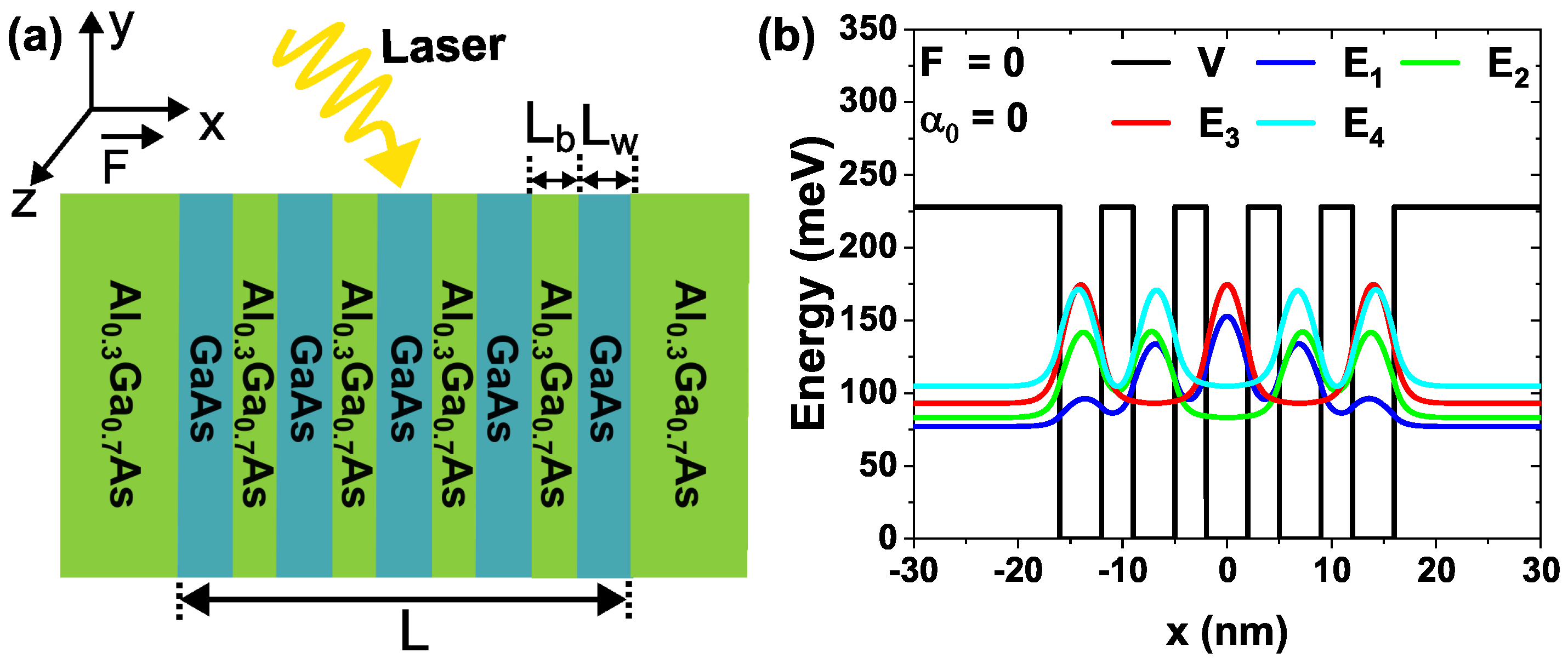
Figure 2.
(a)-(c) Changes in the confinement potential manifest two distinct scenarios for modifications induced by the external fields for the As multiple quantum well system with 4 nm wells and 3 nm barriers: (a) The non-resonant intense laser field dressed the potential, altering the width and height of barriers and wells. (b) The electric field tilts the potential and shifts the charge distribution. In (c), the combined effect for a fixed non-resonant intense laser field of nm and a fixed value of the electric field strength of kV/cm.
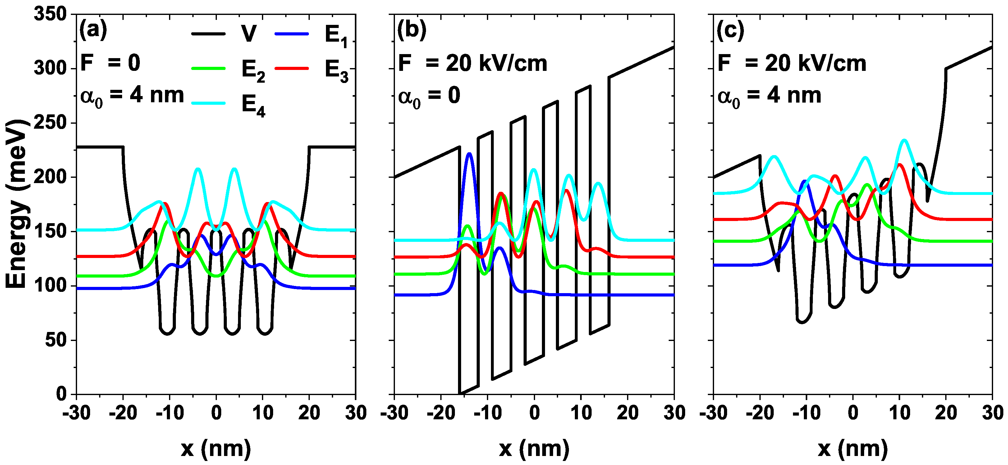
Figure 3.
(a) and (c) The intersubband transition energies as a function of the electric field strength and as a function of the laser-dressing parameter (b) and (d), for the As multiple quantum well system with 4 nm wells and 3 nm barriers. (a) and (b) refer to manipulating the intersubband transition energies by purely electrical and optical means. (c) and (d) show the combined effect of the external fields on the intersubband transition energies for a fixed non-resonant intense laser field of nm (c) and a fixed value of the electric field strength of kV/cm (d). Insets show the energy eigenvalue associated with the first four subbands. Pink circles indicate the intersection between intersubband transition energies.
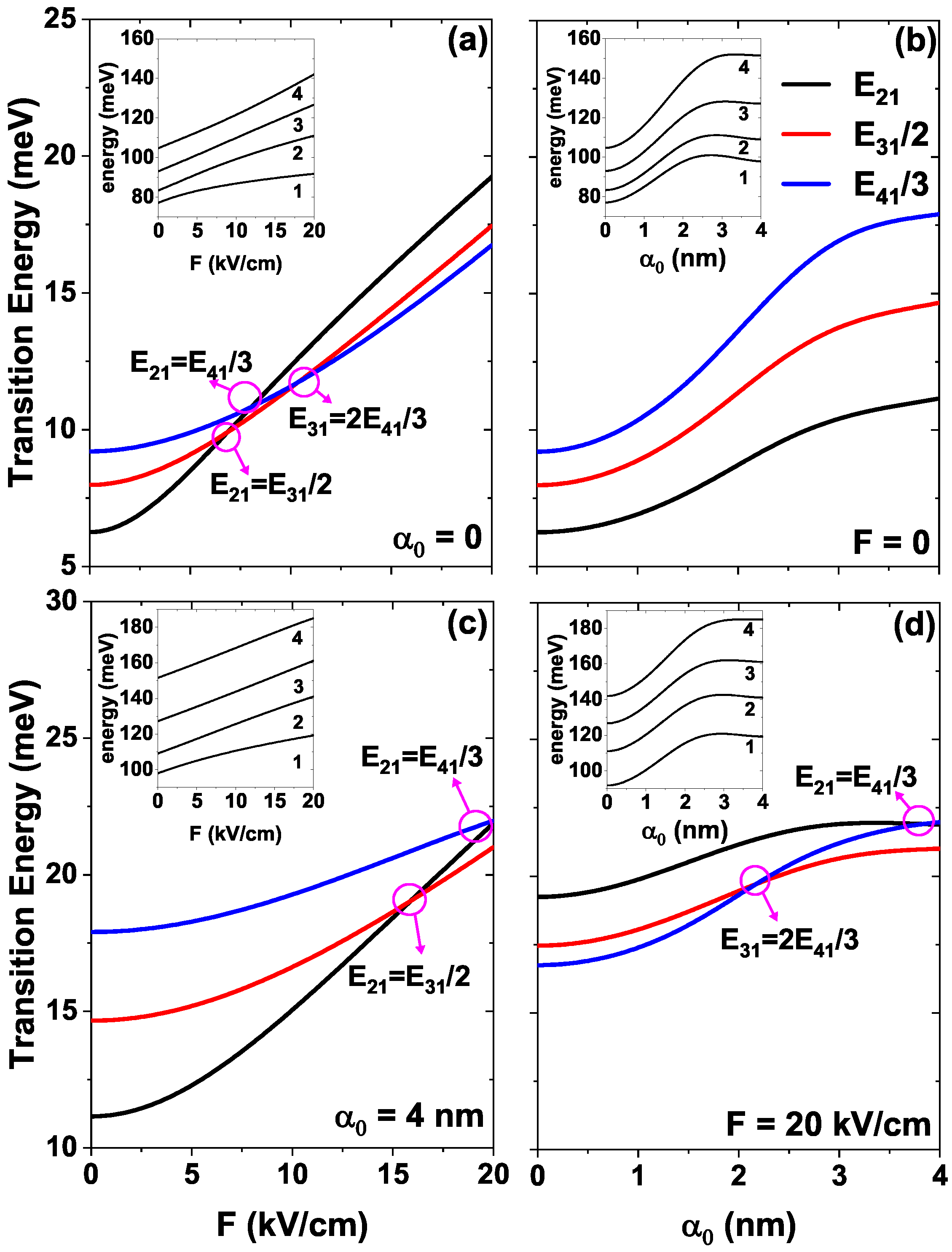
Figure 4.
(a) and (c) The dipole moment matrix elements as a function of the electric field strength and as a function of the laser-dressing parameter (b) and (d), for the As MQWs system with 4 nm wells and 3 nm barriers. (a) and (b) refer to manipulating the intersubband transition energies by purely electrical and optical means, whereas (c) and (d) show the combined effect of the external fields on the dipole moment matrix elements for a fixed nIL field of nm (c) and for a fixed value of the electric field of kV/cm (d).
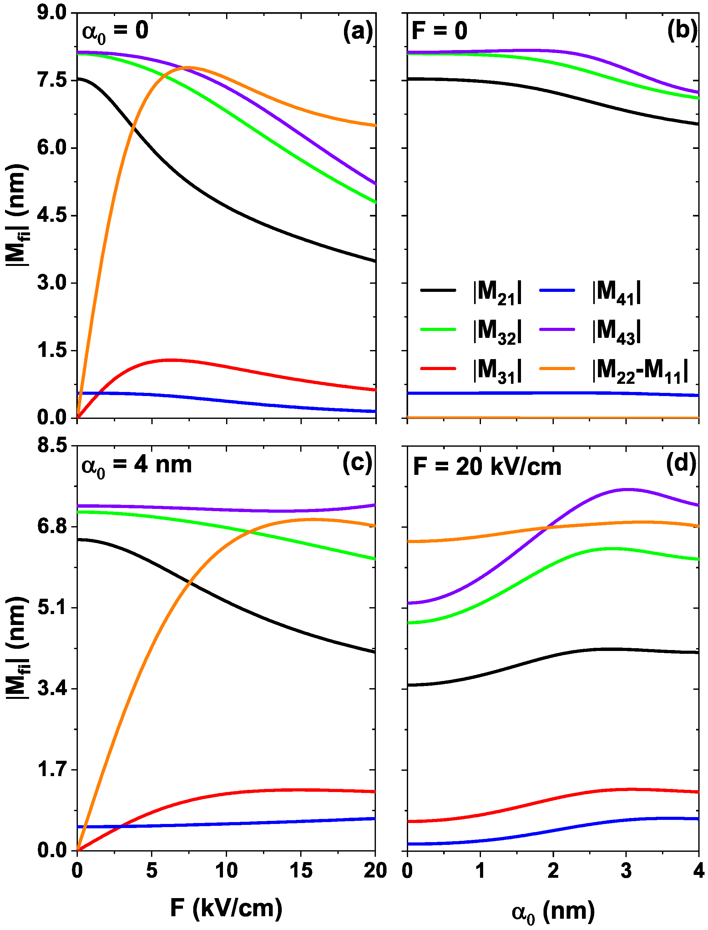
Figure 5.
The geometrical factor as a function of the electric field strength F (a) and as a function of the laser-dressing parameter (b). Dashed lines in (a) and (b) represent the combined electric and non-resonant intense laser field effect, while solid lines stand for a single-field effect.
Figure 5.
The geometrical factor as a function of the electric field strength F (a) and as a function of the laser-dressing parameter (b). Dashed lines in (a) and (b) represent the combined electric and non-resonant intense laser field effect, while solid lines stand for a single-field effect.
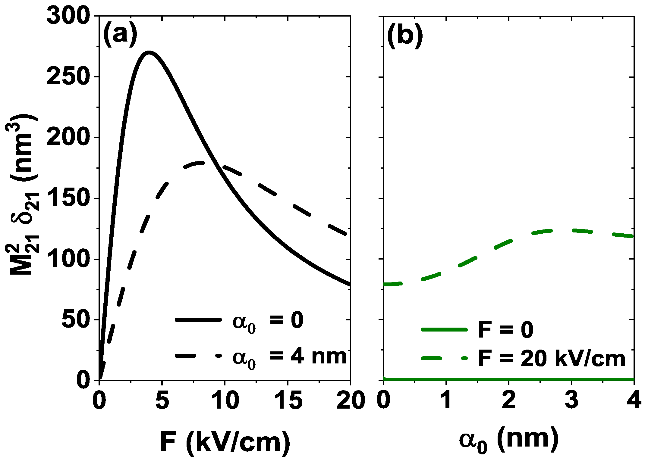
Figure 6.
The geometrical factor as a function of the electric field strength F (a) and as a function of the laser-dressing parameter (b). Dashed lines in (a) and (b) represent the combined electric and non-resonant intense laser field effect, while solid lines stand for a single-field effect.
Figure 6.
The geometrical factor as a function of the electric field strength F (a) and as a function of the laser-dressing parameter (b). Dashed lines in (a) and (b) represent the combined electric and non-resonant intense laser field effect, while solid lines stand for a single-field effect.
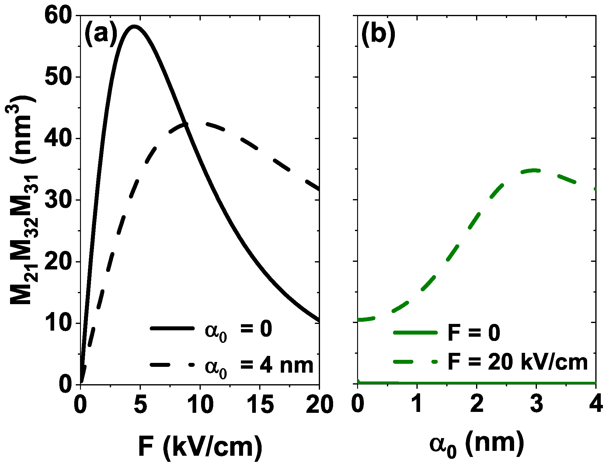
Figure 7.
The geometrical factor as a function of the electric field strength F (a) and as a function of the laser-dressing parameter (b). Dashed lines in (a) and (b) represent the combined electric and non-resonant intense laser field effect, while solid lines stand for a single-field effect.
Figure 7.
The geometrical factor as a function of the electric field strength F (a) and as a function of the laser-dressing parameter (b). Dashed lines in (a) and (b) represent the combined electric and non-resonant intense laser field effect, while solid lines stand for a single-field effect.
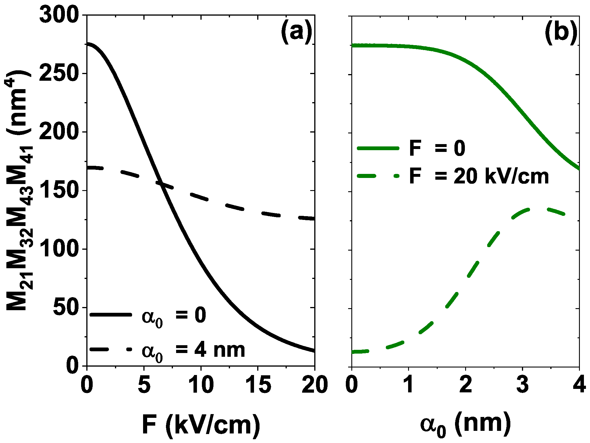
Figure 8.
The nonlinear optical rectification coefficient as a function of the incident photon energy for different values of the electric field strength F at zero non-resonant intense laser field, (a), for nm (b) and for different values of the non-resonant intense laser field parameter at a fixed electric field of kV/cm (c).
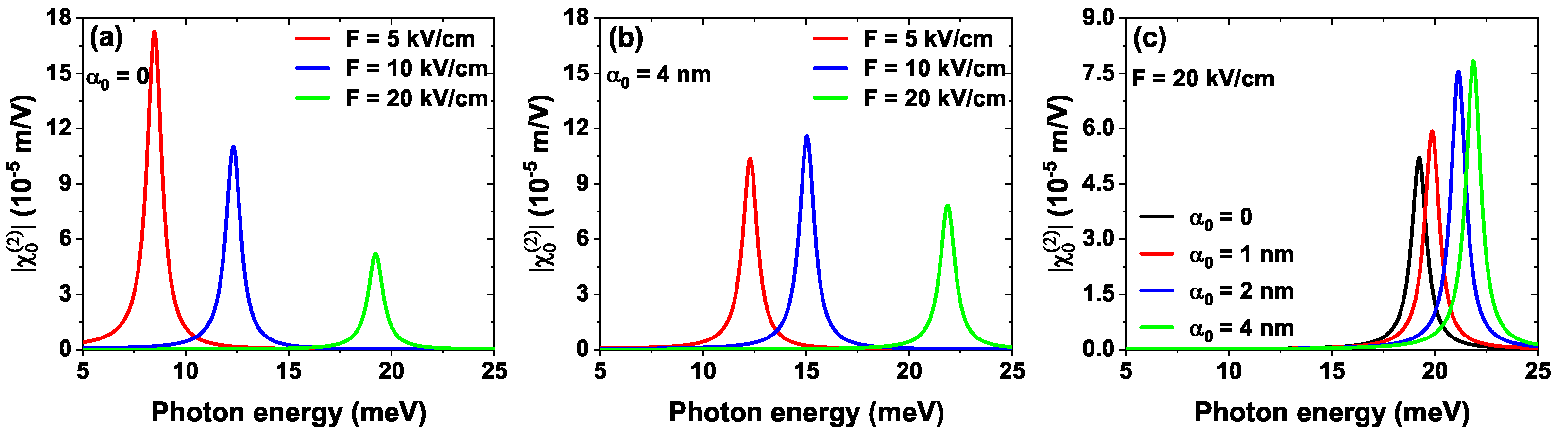
Figure 9.
The second harmonic generation coefficient as a function of the incident photon energy for different values of the electric field strength F at zero non-resonant intense laser field, (a), for nm (b) and different values of the non-resonant intense laser field parameter at a fixed electric field of kV/cm (c). In (a) and (b) the pink curve shows the second harmonic generation coefficient when .
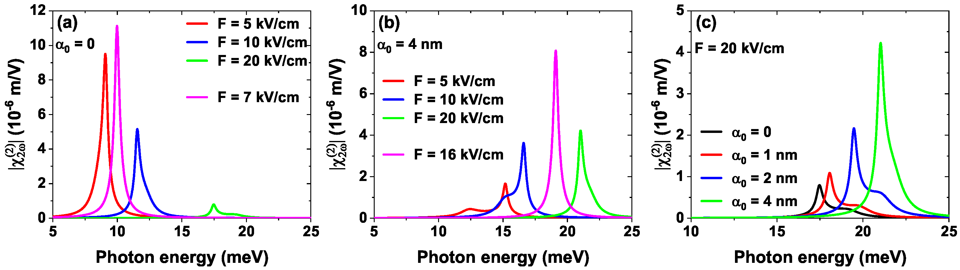
Figure 10.
The third harmonic generation coefficient as a function of the incident photon energy for different values of the electric field strength F at zero non-resonant intense laser field (a) and at nm (b), and for different values of the non-resonant intense laser field without electric field (c) and applying an electric field of kV/cm (d). A factor of 10 is applied to some third harmonic generation coefficient curves to improve their visualization.
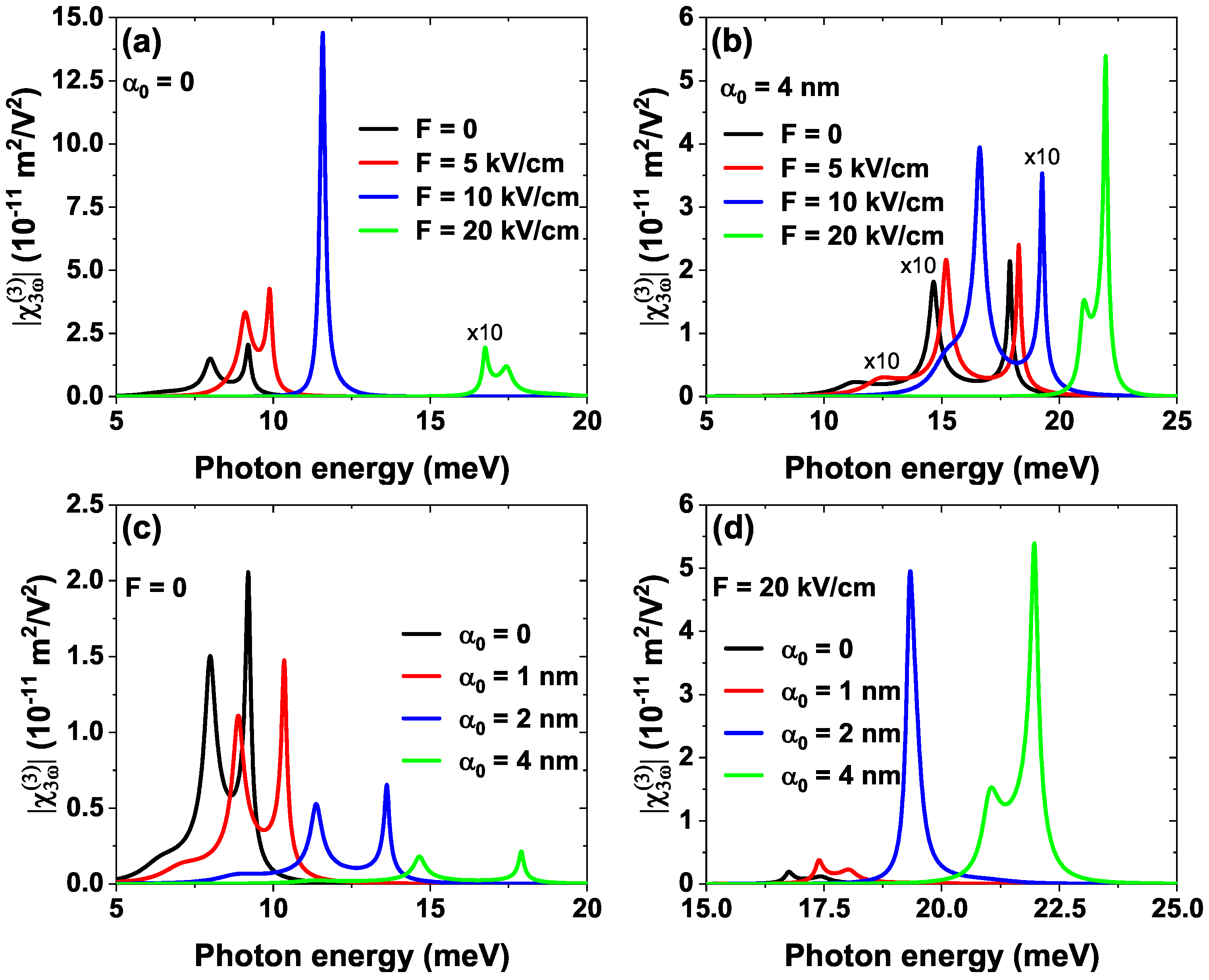

Table 1.
Exact values of the intersubband transition energies varying the electric field strength F and the laser-dressing parameter .
Table 1.
Exact values of the intersubband transition energies varying the electric field strength F and the laser-dressing parameter .
| (nm) | F (kV/cm) | (meV) | (meV) | (meV) |
|---|---|---|---|---|
| 0 | 0 | |||
| 5 | ||||
| 10 | ||||
| 20 | ||||
| 4 | 0 | |||
| 5 | ||||
| 10 | ||||
| 20 |
Table 2.
Exact values of the geometrical factors varying the electric field strength F and the laser-dressing parameter .
Table 2.
Exact values of the geometrical factors varying the electric field strength F and the laser-dressing parameter .
| (nm) | F (kV/cm) | () | ||
|---|---|---|---|---|
| () | () | |||
| 0 | 0 | |||
| 5 | ||||
| 10 | ||||
| 20 | ||||
| 4 | 0 | |||
| 5 | ||||
| 10 | ||||
| 20 |
Disclaimer/Publisher’s Note: The statements, opinions and data contained in all publications are solely those of the individual author(s) and contributor(s) and not of MDPI and/or the editor(s). MDPI and/or the editor(s) disclaim responsibility for any injury to people or property resulting from any ideas, methods, instructions or products referred to in the content. |
© 2025 by the authors. Licensee MDPI, Basel, Switzerland. This article is an open access article distributed under the terms and conditions of the Creative Commons Attribution (CC BY) license (http://creativecommons.org/licenses/by/4.0/).
Copyright: This open access article is published under a Creative Commons CC BY 4.0 license, which permit the free download, distribution, and reuse, provided that the author and preprint are cited in any reuse.


