
Submitted:
04 April 2025
Posted:
07 April 2025
You are already at the latest version
Abstract
Investigating multi-omics data is crucial for unraveling the complex biological mechanisms underlying cancer, thereby enabling effective strategies for prevention, early detection, diagnosis, and treatment. However, predicting patient outcomes through the integration of all available multi-omics data remains an understudied topic. We present SeNMo, a self-normalizing deep neural network trained on multi-omics data across 33 cancer types. SeNMo is particularly efficient in handling multi-omics data characterized by high-width (many features) and low-length (fewer samples) attributes. We trained SeNMo for predicting overall survival of patients using pan-cancer multi-omics data involving 33 cancer sites from the publicly available NCI Genomics Data Commons. The multi-omics data includes gene expression, DNA methylation, miRNA expression, DNA mutations, protein expression modalities, and clinical data. SeNMo was validated on two independent cohorts: Moffitt Cancer Center and CPTAC lung squamous cell carcinoma. The baseline model, trained to predict overall survival, achieved a concordance index (C-Index) of 0.76 in the validation regime and 0.758 on the held-out test set. Furthermore, the model demonstrated strong generalizability, achieving an average accuracy of 99.8% in predicting primary cancer type across pan-cancer cohort. SeNMo further demonstrated significant performance (p< 0.05) in predicting tertiary lymph structures from multi-omics data, showing generalizability across cancer types, molecular data types, and clinical endpoints. SeNMo and similar models are poised to transform the oncology landscape, offering hope for more effective, efficient, and personalized cancer care.
Keywords:
cancer
; oncology
; multi-omics
; multimodal
; pan-cancer
; machine learning
; deep learning
; survival
; classification
1. Introduction
Across the cancer care continuum, from screening, diagnosis, treatment, to survivorship, vast amounts of standard-of-care data are collected from patients. In cancer research, the volume and diversity of data further expand, providing distinct and complementary views of the disease [1]. Studying cancer from a multimodal perspective is essential for comprehensive understanding and for developing effective, personalized treatment strategies [2,3]. The advancement of technologies to record, process, and store molecular data has significantly propelled cancer research [4]. High-throughput sequencing technologies, along with sophisticated bioinformatics tools and computational algorithms, have ushered in an era of “omics" [5]. Multi-omics, a subset of multimodal data, specifically refers to the integrated analysis of various molecular modalities, including genomics, transcriptomics, proteomics, and metabolomics [6,7]. By combining different layers of molecular data, multi-omics transcends the limitations of single-omic studies, which often provide only a partial view of the disease [8,9,10].
Cancer research can be approached from two primary perspectives: individual cancer studies and pan-cancer studies. Individual cancer studies focus on a specific type of cancer, delving deep into its unique molecular and genetic characteristics, allowing for the development of highly targeted therapies and personalized treatment plans. Conversely, pan-cancer studies analyze commonalities and differences across multiple cancer types, uncovering shared molecular mechanisms and genetic alterations. This approach reveals broader patterns and potentially identifies universal biomarkers or therapeutic targets applicable across different cancers, enhancing our holistic understanding of the disease [11]. The pan-cancer perspective has uncovered universal cancer vulnerabilities, detailed pathway alterations for cross-cancer diagnostics and treatments, and revealed shared oncogenic pathways and mutation patterns, leading to new clinically useful insights [11,12]. In this article, we focus on the pan-cancer perspective, emphasizing its potential to generate overarching insights that could lead to more comprehensive and versatile cancer treatment strategies.
2. Literature Review
Existing landscape of Pan-cancer Multi-omics Analysis. Traditionally, multimodal, multi-omics, and pan-cancer studies have been conducted through a variety of techniques and methods that leverage advanced computational, bioinformatics, statistical, machine learning, and deep learning approaches to integrate and interpret complex oncology datasets. Data integration techniques in multi-omics are generally categorized into supervised, weakly supervised, and unsupervised methods. These methods can be further sub-categorized into (1) feature extraction, (2) feature engineering, (3) network-based methods, (4) clustering, (5) factorization, and (6) deep learning techniques [6,13,14,15,16]. Deep learning, a subset of machine learning characterized by neural networks with many layers, has transformed the study of high-dimensional, low-sample molecular data [17,18]. With its capacity to model complex, non-linear relationships and handle vast datasets, deep learning has proven adept at uncovering patterns that traditional statistical and machine learning models may not identify [6,19].
Self-normalizing neural networks have advanced pan-cancer classification, demonstrating superior accuracy and macro F1 scores over random forests using TCGA copy number variation data for LUAD, OV, LIHC, and BRCA, with feature selection crucial for managing high-dimensional data [20]. Integrating histology-genomic data via multimodal deep learning provided deeper cancer insights, with a fusion model outperforming attention-based multiple-instance learning and self-normalizing networks across 14 cancers [21]. DeepProg, an ensemble deep learning and machine learning framework, effectively predicted survival subtypes and risk stratification using RNA-Seq, miRNA sequencing, and DNA methylation data across 32 cancers [22].
Khadirnaikar et al. identified molecularly similar subgroups across 33 tumor types by integrating machine learning and deep learning models, emphasizing the importance of a balanced sample-to-feature ratio for optimal predictive power [23]. A multiview factorization autoencoder predicted progression-free interval and overall survival (OS) using gene expression, miRNA, protein expression, and DNA methylation in TCGA-BLCA and TCGA-LGG [24]. Multi-omics integration (miRNA, mRNA, DNA methylation, lncRNA, and clinical data) improved survival prediction in non-small cell lung cancer, achieving a superior C-Index [25]. Pan-cancer prognostic biomarkers were identified using statistical and bioinformatics methods across 13 cancers, leveraging DNA methylation, gene expression, somatic copy number alterations, and miRNA expression [26].
Multimodal data fusion improved OS prediction across cancer stages and types, with fused models achieving a higher average C-Index than traditional machine learning and bioinformatics methods [27]. This approach integrated clinical, genomic, transcriptomic, and proteomic data across 33 cancers. MCluster-VAEs outperformed in subtype discovery using multi-omics data (mRNA, miRNA, DNA methylation, CNA) across 32 cancers [28]. DEDUCE, a decoupled contrastive learning model with multi-head attention, excelled in subtype clustering using gene expression, DNA methylation, and miRNA data across five cancers (BRCA, GBM, SARC, LUAD, STAD) [29].
Limitations of the State-of-the-art Methods. Although valuable for their intended tasks, the above-mentioned methods often struggle to fully capture the complexity and heterogeneity of cancer due to inherent limitations in handling and interpreting vast, multidimensional datasets. Dimensionality reduction methods such as principal component analysis or t-distributed stochastic neighbor embedding can inadvertently discard subtle yet crucial biological nuances that are pivotal for understanding disease mechanisms [30]. Learning-based dimensionality reduction methods, such as those utilizing deep learning, face challenges including limited discriminative and interpretive capabilities of extracted features, lack of consensus on the balance between the number of network layers and the number of neurons per layer, and limitations in handling or recovering missing data [30].
Similarly, feature selection and learning-based feature engineering, despite being effective in identifying key predictors, can introduce biases and create models that are overly tailored to specific features within training datasets [31,32]. This bias undermines generalizability across diverse datasets or real-world clinical settings [31,32]. Additionally, these methods frequently face challenges in ensuring consistent performance across varied patient populations and biological conditions, limiting their broader clinical utility. Thus, while these techniques are instrumental in advancing cancer research, they underscore the need for more robust and generalizable frameworks capable of accurately predicting endpoints across diverse cancer types and data modalities.
The establishment of large-scale biological databases and data repositories, such as the National Cancer Institute’s TCGA [33] and the Clinical Proteomic Tumor Analysis Consortium (CPTAC) [34], hold vast amounts of multi-omics cancer data that are readily available for disease analysis. Despite numerous efforts, existing literature lacks a model trained on all possible multi-omics pan-cancer data. scGPT is trained for single-cell sequencing data comprising 33 million cells [35]. The SAMMS model was trained on two cancer types (TCGA’s LGG and KIRC) using patient-level data (age, gender), gene expression, CNV, miRNA, and WSI [36]. The RNA Foundation Model (RNA-FM) was trained on 23 million non-coding RNA sequences [37]. PATH-GPTOMIC utilized CNV, genomic mutations, bulk RNA Seq, and WSI data to predict survival outcomes for two datasets (TCGA-GBMLGG, TCGA-KIRC) [38]. The absence of a pan-cancer, multi-omics model can be attributed to challenges such as data complexity, heterogeneity, limited comprehensive datasets, specificity of analytical methods, and large computational demands. To address these challenges, we propose a multi-omics, pan-cancer framework, called the ’Self-Normalizing Deep Learning Model for Multi-Omics’ (SeNMo). SeNMo has been trained on six data modalities, including clinical, gene expression, miRNA expression, DNA methylation, DNA mutations, and reverse-phase protein array (RPPA) expression data across 33 cancer types. We evaluated SeNMo’s generalization capability to unseen datasets and across different tasks such as OS prediction, primary cancer classification, and tertiary lymph structures (TLS) ratio prediction. Figure 1 presents the overview of our framework.
This work offers the following contributions:
- The SeNMo framework represents the first initiative to analyze 33 cancer types using five molecular data modalities: gene expression, miRNA expression, DNA methylation, DNA mutations, and protein expression, along with the clinical data.
- We created a multi-omics, pan-cancer framework with minimal and essential preprocessing steps, eliminating the need for complex, custom-engineered methods, thereby allowing a greater focus on the learning aspect.
- We developed a deep learning model capable of generalizing across different tasks and to unseen data through fine-tuning.
- Our findings indicate that MLP-based networks are highly susceptible to catastrophic forgetting. We demonstrate that fine-tuning should involve a fraction of the epochs (), while adjusting the learning rate, weight decay, and dropout to fractionally update all layers of the trained model.
- We present the first effort to predict tertiary lymph structures (TLS) ratio from multi-omic data only.
- We provide the latent feature vectors (embeddings) learned by SeNMo as an open-access vector database system, HoneyBee, available through Hugging Face and GitHub, and separately through Zenodo.
3. Materials and Methods
3.1. Data Acquisition
TCGA houses one of the largest collections of high-dimensional multi-omics datasets, comprising over 20,500 individual tumor samples from 33 different cancer types [33]. The available data includes high-throughput RNA sequencing (RNA-Seq), DNA sequencing (DNA-Seq), microRNA sequencing (miRNA-Seq), single nucleotide variants, copy number variations, DNA methylation, and reverse-phase protein array (RPPA) data [33]. Building cohorts from this diverse data, spanning multiple formats, modalities, and systems, presents significant challenges. To curate and establish patient cohorts, we utilized our previously developed Multimodal Integration of Oncology Data System (MINDS), a metadata framework designed to fuse data from publicly available sources like TCGA-GDC and UCSC Xena Portal into a machine learning-ready format [33,39,40]. MINDS is freely accessible to the cancer research community, and has been integrated into the SeNMo framework to enhance its usability and benefit to researchers. For training, validation, and testing, we used pan-cancer data from TCGA and Xena, covering 33 cancer types, as summarized in Table 1. We further fine-tuned the model using data from the CPTAC-LSCC [41] and Moffitt’s LSCC datasets [42] to evaluate the generalizability and transfer learning capabilities of SeNMo.
3.2. Data Modalities
From the 13 available modalities present in each cancer dataset, we selected gene expression (RNAseq), DNA methylation, miRNA stem-loop expression, RPPA data, DNA mutation, and clinical data. These modalities were chosen based on their frequent use in cancer studies due to their direct relevance to the fundamental processes of cancer progression, as well as their diagnostic and prognostic capabilities [43,44]. Furthermore, these selected modalities provide robust predictive and prognostic information, and their integration gives a holistic view of a tumor’s multi-omic profile [43,44,45]. Importantly, each modality had a consistent number of features across all cancer types, which facilitated the development of a standardized data preprocessing pipeline for pan-cancer studies. TCGA-GDC multi-omics data includes DNA methylation (485,576 CpG sites, beta values 0-1), gene expression (RNAseq) (60,483 features, HTseq-FPKM values log-transformed after incrementing by one, with high expression >1000 and low between 0.5-10), miRNA stem-loop expression (1880 features, log-transformed values), protein expression (RPPA data profiling 500 proteins, normalized via log transformation and median centering), DNA mutation (18,090 mutational features from MAF files summarizing somatic mutations), and clinical data (patient covariates like age, gender, race, and cancer stage, essential for prognosis and treatment response). For details on each modality, see supplementary Appendix A.
3.3. Pre-Processing
Multiomics data integrates diverse biological data modalities such as genomics, transcriptomics, proteomics, and metabolomics to study complex diseases like cancer but requires extensive preprocessing due to the big P, small n problem—high dimensionality (P) with limited samples (n) [46]. The pan-cancer multi-omics data comes with intra- and inter-dataset correlations, heterogeneous measurement scales, missing values, technical variability, and other background noise. Preprocessing challenges include data heterogeneity, large volume and complexity, quality and variability, missing values, and lack of standardization across studies. Effective preprocessing involves normalization, scaling, handling missing data, dimensionality reduction, data annotation, metadata inclusion, and selecting appropriate integration techniques to ensure data is machine learning-ready. Addressing these challenges requires interdisciplinary expertise, including bioinformatics, statistics, and domain-specific knowledge. Here, we describe the preprocessing steps used across molecular data modalities.
- Remove NaNs. First, we removed the features that had NaNs across all the samples. This reduced the dimension, removed noise, and ensured continuous-numbered features to work with.
- Drop constant features. Next, constant/quasi-constant features with a threshold of 0.998 were filtered out using Feature-engine, a Python library for feature engineering and selection [47]. This eliminated features with no expression at all across every sample along with features that were noise, since the expression value was the same across every sample.
- Remove duplicates features. Next, duplicate features between genes were identified that contained the same values across two seperate genes, and one of the genes was kept. This may reveal gene-gene relationships between the two genes stemming from an up-regulation pathway or could simply reflect noise.
- Remove colinear features. Next, we filtered the features having low variance (≈0.25) because the features having high variance hold the maximum amount of information [48]. We used VarianceThreshold feature selector of scikit learn library that removes low-variance features based on the defined threshold [49]. We chose a threshold for each data modality so that the resulting features have matching dimensions, as shown in Figure 2.
- Remove low-expression genes. The gene expression data originally contained 60,483 features, with FPKM transformed numbers ranging from 0 to 12. Roughly 30,000 features remained after the above-mentioned preprocessing steps, which was still a very high number of features. High expression values reveal important biological insights due to an indication that a certain gene product is transcribed in large quantities, revealing their relevance. Features containing an expression value greater than 7 (127 FPKM value) were kept, while the rest were discarded.
- Handle missing features. We handled missing features at two levels of data integration. First, for the features within each modality and cancer type, the missing values were imputed with the mean of the samples for that feature. This resulted in the full-length feature vector for each sample. Second, across different cancers and modalities, we padded the missing features with zeros. In deep learning, the zero imputation technique shows the best performance compared to other imputation techniques and deficient data removal techniques [50,51,52].
3.3.1. Features Integration
After preprocessing, the data is integrated across cancers and modalities, generating two views: one by unifying features across all patients within each modality, and second by combining all modalities. Feature dimensions post-preprocessing include DNA methylation (reduced from 485,576 to ∼4,500 per patient, unionized to 52,396), gene expression (60,483 to ∼3,000 per patient, unionized to 8,794), miRNA expression (1,880 to ∼1,400 per patient, unionized to 1,730), protein expression (487 to 472), and DNA mutation (18,090 to 17,253). Clinical categorical features like gender, race, and cancer stage are converted to numerical values for integration. The details of these clinical characteristics are given in Table 2. Mathematically, the preprocessing is given below.
Let v represent the initial feature having fixed dimension for each cancer. The dimension of each feature set is reduced through a preprocessing step, resulting in the feature vector , which is calculated by a function of v, noted as , where f is the dimension reduction function such as those presented in the previous section, . For cancer types, the reduced dimensional feature vector from each cancer type are then combined through a union operation to generate a feature vector for each modality m and are the total number of modalities. The feature vector for each modality, , is defined as:
Finally, the union of all across different modalities results in the total pan-cancer, multimodal feature vector , expressed as:
3.4. Clinical End-Points
To assess the performance of the SeNMo framework, we selected three clinical end-points that fall under two categories of machine learning tasks. The first end-point is Overall Survival (OS), which is treated as a regression task. The second is the prediction of primary cancer type, formulated as a 33-class classification task. The third end-point is TLS ratio prediction, also a regression task.
3.4.1. Overall Survival (OS)
Predicting cancer prognosis through survival outcomes is a standard approach for biomarker discovery, patient stratification, and assessing therapeutic response [53]. Advances in statistical survival models and deep learning have improved OS prediction by integrating molecular and clinical data [25,54]. In this study. we analyze clinical, demographic, and genomic factors to assess their correlation with patient survival, implementing OS prediction as a regression task in days. Survival data includes time-to-event records, accounting for right censoring when exact survival times are unknown. Figure 3A illustrates survival times since cancer diagnosis for the pan-cancer dataset. Each patient’s outcome is characterized by two variables: a censoring indicator, also known as the vital status, and the observed time , where represents the true survival time and is the censoring time, [55]. The survival function, which describes the probability that a patient will survive beyond a specified time t, is given by:
Additionally, the hazard function provides insight into the risk of an event occurring at a particular time, given survival up to that point. It represents the instantaneous rate of events (e.g., death) occurring at a specific time, conditional on having survived to that time. The hazard function is mathematically defined as the ratio of the probability of the event occurring in a short interval around t to the probability of surviving beyond t:
where, is the hazard function at time t, T is the survival time, is the conditional probability that the event occurs in the time interval given that survival time is greater than or equal to t, and represents an infinitesimally small time interval. Based on survival data, the hazard function describes the instantaneous risk of experiencing the event of interest at any given time. In our study, right-censoring was defined as censor in case of an event (e.g., death), and 0 otherwise.
3.4.2. Primary Cancer Type
Classifying primary cancer type based on biological and clinical features is critical for accurate treatment selection, improving patient outcomes, and enabling personalized therapies [56]. Since treatments and prognoses vary across cancer types, precise classification supports tailored interventions, follow-up care, and early recurrence detection. High classification accuracy enhances clinical decision-making, ultimately benefiting patient survival and quality of life. The distribution of patient samples across 33 cancer types is shown in Figure 3.
3.4.3. Tertiary Lymphoid Structures (TLS) Ratio
TLSs are immune cell aggregates resembling secondary lymphoid organs, forming in inflamed tissues, including cancers, and are associated with improved survival and immunotherapy response [57,58]. The TLS ratio (segmented TLS area/total tissue area) serves as a prognostic biomarker, influencing clinical decision-making. Automated TLS segmentation models have shown high accuracy across multiple cancers [57,58]. In this study, whole slide images of H&E and CD20-stained sections were analyzed using Visiopharm 2022.03. Visiopharm Tissuealign co-registered serial images, tumor and non-tumor regions were manually segmented, and TLSs were detected via thresholding, followed by manual review and feature extraction by an experienced image analysis technician under pathologist supervision.
3.5. SeNMo Deep Learning Model
In scenarios involving hundreds or thousands of features with relatively few training samples, feedforward networks often face the risk of overfitting [53]. Unlike CNNs, weights in feedforward networks are shared, making them vulnerable to training instabilities caused by perturbations and regularization techniques such as stochastic gradient descent and dropout. CNNs, on the other hand, struggle to handle high-dimensional, low-sample data due to the spatial invariance assumption, fixed input size, and inefficiencies in managing multi-omics data sparsity. Transformer-based models are also suboptimal for high-dimensional, low-sample data, as they rely heavily on attention mechanisms tailored for predicting sequential patterns, which fails when dealing with highly sparse molecular data. To address the challenges of overfitting and instability in high-dimensional, low-sample-size multi-omics data, we drew inspiration from self-normalizing networks introduced by Klambauer et al. [59]. Self-normalizing neural networks are particularly suited for high-dimensional datasets with limited samples, a characteristic that makes them highly relevant for multi-omics analysis. The SeNMo architecture is based on stacked layers of self-normalizing neural networks, as detailed below.
SeNMo comprises stacked blocks of self-normalizing neural network layers, where each block includes a linear unit, a Scaled Exponential Linear Unit (SELU) activation, and Alpha-Dropout. These components enable high-level abstract representations while keeping neuron activations close to zero mean and unit variance [59]. The linear unit is equivalent to a “fully connected" or MLP layer commonly used in traditional neural network architectures. Klambauer et al. demonstrated through the Banach fixed-point theorem that activations with close proximity to zero mean and unit variance, propagating through numerous network layers, will ultimately converge to zero mean and unit variance [59]. SELU activations, an alternative to traditional rectified linear unit activations, offer a self-normalizing effect, ensuring activations converge to zero mean and unit variance regardless of the input distribution. The SELU activation function is expressed mathematically as:
where, is a scaling factor (typically set to ) and is the negative scale factor (typically set to ).
Dropout, a regularization method that randomly sets a fraction of input units to zero during training, prevents overfitting. Alpha-Dropout, a modified version of traditional dropout, is designed to maintain the self-normalizing property of SELU activations. It applies a dropout mask during training, scaled to ensure the mean and variance of activations remain stable. The scaling factor is computed based on the dropout rate and the SELU parameters ( and ). Alpha-Dropout is mathematically defined as:
where, x is the input activation, , are mean and standard deviation of the input activation, respectively, and is a binary mask generated with the specified dropout rate.
Together, SELU activations and Alpha-Dropout ensure that SeNMo blocks maintain stable mean and variance across network layers, facilitating more reliable training and better generalization performance. Additionally, these mechanisms help mitigate training instabilities related to vanishing or exploding gradients in feedforward networks. Our network architecture consists of seven fully connected hidden layers, each followed by SELU activation and Alpha-Dropout. The final fully connected layer is used to learn a latent representation of each sample, termed as the patient embedding .
3.6. Training and Evaluation
3.6.1. Data Splits
For the OS task, the pan-cancer data was randomly divided into the training-validation set () and the hold-out test set () for each cancer type. The pan-cancer training was carried out by combining the training-validation cohort of all 33 cancer types and adopting the 10-fold cross-validation with the division of samples. The training-validation cohort has patients, each having features, comprising the six modalities mentioned earlier. For the evaluation/testing of the trained model, the inference data was created by combining the held-out test set from all 33 cancer types, resulting in patients. We tested the optimal hyperparameters of our trained model to train different combinations of the pan-cancer data modalities. We call these 1-modal, 3-modal (gene expression, DNA methylation, miRNA expression), 4-modal (protein expression), 5-modal (DNA mutation), and 6-modal (all modalities) cohorts. Although our initial model was trained on all 6 modalities, these experiments aim to see how the model performs on each of these pan-cancer cohorts where one or more of the data modalities is missing.
3.6.2. Evaluation
We evaluate SeNMo’s performance with the quantitative and statistical metrics common for survival outcome prediction and classification. For survival analysis, we evaluated the model using the C-index. For the primary cancer type classification, we generate the classification report comprising average accuracy, average precision, recall, F1-score, confusion matrix, and scatter plot. For the TLS Ratio, we employed Huber Loss. We utilized the log-rank test to determine if the survival predictions were statistically significantly different. For details on each evaluation metric, see supplementary Section B.
3.7. Study Design
An overview of the various simulations conducted to evaluate the capabilities of the SeNMo model across different learning regimes, tasks, and datasets is shown in Figure 4. The study design included multiple learning regimes, each designed to assess the model’s adaptability, generalizability, and robustness. The baseline model was initially trained on TCGA dataset comprising 33 different cancer types for OS prediction. The subsequent learning regimes explored different data variations and tasks, which we call out-of-distribution simulations because the model had not encountered such data/task in baseline learning. These scenarios included OS prediction on both seen and unseen datasets, as well as tasks such as primary cancer type classification on seen data and TLS ratio prediction on unseen data.
4. Results
4.1. Pan-Cancer Multimodal Analysis for Predicting OS
Figure A1 shows the visualization of the parallel sweeps across all hyperparameters, resulting in training around 400 unique models. The optimal model had a learning rate of , a weight decay of , dropout, 256 batch size, 100 epochs, and seven hidden layers with neurons in these layers as . The trained model contained million trainable parameters. Checkpoints were saved for this model for each of the 10 folds. The model’s training resulted in the average training C-Index of and average validation C-Index of across the 10 folds. The inference on the test set showed the C-Index of , the average of the C-Indices from the 10 checkpoints. To further validate our findings, we created an ensemble of the 10 checkpoints by averaging the prediction vectors from all the models and then evaluating the final averaged prediction vector for C-Index. For the pan-cancer, multi-omics SeNMo model, an ensemble C-Index of was achieved on the held-out test set. The significance level in all these analyses is , i.e., , indicating statistically significant values. These results are depicted in the Figure 5.
As depicted in Figure 5, the SeNMo model trained on the pan-cancer 1-modal (Gene expression) cohort showed a C-Index for training, validation, testing, and ensemble inference as and , respectively. For the pan-cancer 1-modal (DNA methylation) cohort, the model’s training, validation, testing, and ensemble inference C-indices are and , respectively. For the pan-cancer 1-modal (miRNA expression) cohort, the model’s training, validation, testing, and ensemble inference C-indices are and , respectively. We did not analyze the model individually on the rest of the three modalities because clinical and protein expression features are too small for an 83 million-parameter model, whereas the DNA mutation data comprised the binarized features of mutations. Evaluating the model on the 3-modal cohort showed the training, validation, testing, and ensemble inference C-indices of and , respectively. Further adding the protein expression to the 3-modal data, we trained and evaluated the model on the 4-modal cohort and got the C-Indices of and for training, validation, testing, and ensemble inference, respectively. Lastly, the model’s performance on the 5-modal cohort showed the training, validation, testing, and ensemble inference C-indices of and , respectively. Next, we analyze how the model trained on pan-cancer, 6-modal data fared on individual cancer patients’ data.
4.2. Individual Cancer Multimodal Analysis for Predicting OS
We evaluated the model trained on the 6-modal pan-cancer cohort on the held-out individual cancer data from an individual cancer-wise perspective. The number of patients in these cancer cohorts was a randomly selected subset of the cases shown in Figure 3 and Table 1, Table 2, which accounts for the of the total samples. The trained model was evaluated on each of the 33 individual cancer data using simple inference and the ensemble of the 10-fold checkpoints. Figure 6 shows the evaluation performance of the model on 33 cancer types. The model showed the best predictive performance on TCGA-PCPG data with an average C-Index on the test set of and ensemble inference of . SeNMo’s performance on the other cancer types in format {Test Inference, Ensemble Inference} is shown in Table 3, where 29 cancer types have significant C-Indices. We noticed that the results for TCGA-GBM, TCGA-LAML, TCGA-PRAD, and TCGA-TGCT were not statistically significant, i.e., . So, we fine-tuned the model for these datasets by reducing the learning rate, increasing the weight decay and dropout, and letting the model fine-tune for 10 epochs. Resultantly, the model’s performance increased for TCGA-GBM, TCGA-LAML, and TCGA-PRAD. These improvements are depicted with the green arrows and green boxes in Figure 6. However, the model failed to converge for TCGA-TGCT data and consistently gave predictions that were not significant, .
4.3. Out-of-Distribution Evaluation and Fine-Tuning
Evaluating the model without fine-tuning showed the {Test Inference, Ensemble Inference} of CPTAC-LSCC, and Moffit-LSCC. Fine-tuning the model for 10 epochs, with reduced learning rate, and increased weight decay and dropout resulted in the improvement of C-Indices as CPTAC-LSCC, and Moffit-LSCC. These fine-tuning results are depicted in Figure 6 as the green box plots.
4.4. Patient Stratification
We further investigated the SeNMo’s ability to stratify the patients based on low, intermediate, and high risk conditions. We generate Kaplan-Meier (KM) curves of our model on the pan-cancer, multi-omics held-out test set, as shown in Figure 7. We select the low/ intermediate/ high risk stratification distribution as the 33-66-100 percentile of hazard predictions [53,60]. The hazard scores predicted by SeNMo are used to evaluate the model’s stratification ability. The KM comparative analysis shows that SeNMo distinguished the patients across the three groups. The low-risk group (green) exhibited the highest survival probability, maintaining close to 100% survival up to approximately 5 years, and gradually declining to about 60% by the 25-year mark. The intermediate-risk group (blue) showed a significantly lower survival probability, starting to diverge from the low-risk group early on and reaching around 40% by the 15-year mark of the study period. The high-risk group (orange) displayed the most pronounced decline in survival probability, with a steep drop to approximately 20% survival within the first 10 years, and further reducing to below 10% after 10 years. The logrank test to evaluate the significance of this stratification shows that the p-value of low vs. intermediate curves is , low vs. high is , and intermediate vs. high is , showing significant results, i.e., . The 95% confidence intervals around each curve show the reliability of these estimates.
4.5. Primary Cancer Type Prediction
To test the generalizability of SeNMo across different tasks, we carried out the prediction of primary cancer type from pan-cancer, multi-omics data. We set the problem as a classification problem, where the multi-omics data is used to predict the type of cancer for the given patient data among the 33 classes. It is imperative to mention here that the four clinical features in the initial data contained the cancer stage, as shown in Figure 2 and Table 2. When considering a cancer type classification problem, the stage adds a bias in the data because of the staging distribution among different cancers. Therefore, for the cancer classification simulations, we excluded the “stage” feature in the clinical data. As shown in Figure 8, the model achieves near-perfect accuracy levels, with 99.9% average accuracy in training, 99.8% in validation, and consistent performance in both simple and ensemble inference approaches. The confusion matrix depicts a clear concentration of values along the diagonal, indicating a high rate of correct predictions across all cancer types. The scatter plot shows an alignment of predicted labels with true labels along the diagonal line, highlighting the model’s robust predictive accuracy. The classification report across various cancer types reveals that the model consistently maintains high precision, recall, and F1-scores, approaching a value of 1 for almost all categories. The robust predictive power of our model emphasizes the fact that each cancer has a unique molecular landscape, highlighted through differences in gene, protein, and miRNA expression, DNA methylation, and types of somatic mutations seen in our data.
4.6. Tertiary Lymph Structures (TLS) Ratio
To further evaluate SeNMo’s generalizability on previously unseen data and across different tasks, we fine-tuned the model to predict the TLS ratio on a cohort of lung squamous cell carcinoma data collected at Moffitt Cancer Center. This task was formulated as a regression problem. As shown in Figure 9, the TLS ratio predictions generated by SeNMo demonstrated strong performance on the held-out test set. Specifically, the comparison between manual TLS ratio annotations and SeNMo-predicted ratios revealed no significant difference (), indicating a high level of concordance between manual assessments and model predictions (Figure 9b). Further analysis using violin plots compared the distribution of TLS ratios for manually annotated high vs. low groups with those predicted by SeNMo. Both manual and predicted TLS ratios showed significant separation between high and low groups (), highlighting the model’s ability to accurately distinguish between different levels of TLS (Figure 9c and Figure 9d). Moreover, KM survival analysis was performed to assess the prognostic value of TLS ratios. Survival curves revealed significant differences in survival outcomes between patients with high and low TLS ratios, both for manually annotated data () and SeNMo-predicted data () (Figure 9e).
5. Discussion
We analyzed pan-cancer dataset of 33 cancer types comprising five molecular data modalities (with varying amount of features) and four clinical data features using our SeNMo encoder-based framework. Public databases such as CPTAC and TCGA contain common identifiers within their data that connect data from the same patient. Therefore, molecular data, such as gene expression, miRNA expression, DNA methylation, somatic mutations, and protein expression can be consolidated to represent a singular patient. However, such high-dimensional data has intra- and inter-dataset correlations, heterogeneous measurement scales, missing values, technical variations, and other forms of noise [55]. This necessitates the need for a variety of preprocessing techniques such as the removal of low variance features and the imputing of missing features among others prior to training. Training such a large dataset having high-dimensional heterogeneous data required proper computational resources and a precise pipeline for training, testing, and validation. After extensive training-evaluation runs, we found, through optimal parameters searching, a model that performs very well across the different data types and tasks (refer to Figure 5 and Figure A1). The model has been shown to outperform the existing works in OS prediction when considering the six data modalities included in our data [27]. Moreover, we observed that adding more data and types of modalities increased the model’s performance.
The model’s performance was evaluated on individual cancers at test-time through simple inference and ensembling methods. We observed that the model’s predictive power improved when an ensemble of the checkpoints was employed, (refer to Figure 6). However, for four cancer types, TCGA-GBM, TCGA-LAML, TCGA-PRAD, and TCGA-TGCT, the model did not show significant predictive power. During the investigation, we observed that these datasets had non-admissible pairs in some of the data folds, i.e., all samples had censor value in Equation 10. In the case of TCGA-PRAD and TCGA-TGCT, the number of samples having in the training/validation cohort was 12 and 3, respectively. To address the lack of predictive power, we fine-tuned the model for these datasets by using the stratified k-folds to offset the class-representation problem in the data folds. After searching for the optimal hyperparameters for fine-tuning, the model’s performance became significant () for three out of four datasets, (refer to green box plots in Figure 6).
It is imperative to mention here that MLPs-based networks are very sensitive to catastrophic forgetting when presented with out-of-distribution data or when subjected to a different task [61]. We fine-tuned the SeNMo encoder for one public data (CPTAC-LSCC) and one internal data (Moffitt’s LSCC) [41,42]. In our simulations to fine-tune the model, we encountered the catastrophic forgetting phenomenon in SeNMo, where the model would fail to converge on both new datasets. This was more pronounced when a certain number of hidden layers were frozen, and the rest were trained with lower learning rates. We resorted to the option of unfreezing all the layers of the encoder and fine-tuning the model with a very small learning rate (), high weight decay and dropout (), and just 10 epochs. This method worked and the model showed significant performance on the out-of-distribution datasets.
Risk stratification of patients allows clinicians and researchers to identify patients who might need more intensive care or monitoring and those who may have a better prognosis, facilitating more personalized treatment approaches. The KM survival curves depicted in Figure 7 demonstrate a clear stratification of survival probabilities among three risk-defined patient groups. These results underscore the effectiveness of the risk stratification model in predicting long-term outcomes and highlight the critical need for targeted therapeutic strategies based on individual risk assessments. This stratification allows for more personalized patient management and could potentially guide clinical decision-making toward improving OS rates across diverse patient populations.
Cancer type classification is routinely studied for early detection and localization of tissue of origin [62]. The classification results in Figure 8 illustrate the superior generalizability of the model’s predictive power to classify primary cancer types through the SeNMo encoder, despite it being primarily trained for predicting OS. Additionally, the detailed classification report across various cancer types reveals that the model consistently maintains high precision, recall, and F1-scores for almost all cancer types. Such metrics not only confirm the model’s effectiveness in accurately identifying the correct cancer class but also its reliability in replicating these results across different samples. This level of performance suggests the capability of the model to successfully learn high level representations from heterogenous, high-dimension, mutlivariate data stemming from complex molecular modalities such as gene expression, miRNA expression, somatic mutations, DNA methylation, and protein expression.
As shown in Figure 9, SeNMo’s ability to predict TLS ratios was evaluated on an unseen cohort of lung squamous cell carcinoma data from Moffitt Cancer Center. The comparison between manual TLS ratio annotations and SeNMo-predicted values showed no significant difference, indicating a high level of concordance between human annotations and model predictions. Violin plots depicting high vs. low TLS ratio groups—both for manual and SeNMo predictions—revealed significant separation, demonstrating the model’s robustness in distinguishing between biologically distinct TLS levels. Furthermore, KM survival curves for high vs. low TLS ratio groups revealed significant differences in survival outcomes, with stronger statistical significance observed for SeNMo-predicted data compared to manual annotations. These results underscore the potential of SeNMo to not only replicate expert-driven TLS annotations but also provide a consistent and potentially superior prognostic assessment. Overall, the results indicate that SeNMo can successfully generalize to new tasks and datasets, accurately predicting TLS ratios and offering valuable prognostic insights that could improve clinical decision-making.
5.1. Limitations of the Study
The SeNMo model failed to converge for the TCGA-TGCT data (). The authors argue that a possible rationale is due to the more pronounced class imbalance in this particular dataset, i.e., 3 out of 111 samples in the training cohort have censor value , the model cannot learn to distinguish the samples based on the OS. Moreover, we have not included copy number variations and other molecular data modalities in this analysis, which can be undertaken as a prospective future work.
6. Conclusion
In this study, we introduced SeNMo, a deep learning model specifically designed for multi-omics data analysis across 33 different cancer sites. By leveraging high-dimensional multi-omics datasets from the NCI Genomics Data Commons, SeNMo demonstrated robust performance in predicting overall survival on both training and held-out test sets. The model’s adaptability and efficiency were further validated through its high accuracy in classifying primary cancer types and predicting TLS ratios, showcasing its ability to generalize effectively across different tasks. SeNMo represents a resilient and scalable solution that advances the integration and analysis of complex molecular data, providing a comprehensive understanding of cancer biology. Our approach underscores the potential of self-normalizing networks in oncology, emphasizing the importance of comprehensive data preprocessing and optimal parameter tuning. By making SeNMo and its derived patient embeddings publicly available, we aim to facilitate further research and innovation in personalized cancer care, underscoring the transformative potential of multi-omics approaches in the fight against cancer.
Author Contributions
A.W., A.T., S.A., H.F., M.S., P.S., M.N., G.R. conceived the idea, A.W., A.T., S.A., A.M., M.S., P.S., G.R. are responsible for conceiving, writing and evaluating the implementation and simulations in Python, G.R., P.S., M.S., M.N. verified the concept, implementation, methodology, and results. A.W., A.T., S.A., A.M. wrote the initial draft manuscript. All authors have read and approved the manuscript.
Funding
This work has been supported in part by the National Science Foundation awards 1903466, 2008690, 2234836, 2234468, NIH grant U01CA200464, grant from the State of Florida Bankhead Coley Research Program (21B12), and in part by the Biostatistics and Bioinformatics Shared Resource at the H. Lee Moffitt Cancer Center & Research Institute, an NCI-designated Comprehensive Cancer Center (P30-CA076292).
Data Availability Statement
The molecular data, overall survival information, and other phenotypes from the TCGA and corresponding labels are available from NIH Genomic Data Commons (https://portal.gdc.cancer.gov/). The gene expression, miRNA expression, and DNA Methylation data was obtained from UCSC XENA (https://xena.ucsc.edu/). The CPTAC-LSCC and Moffitt LSCC data are available at [40,42]. The codebase for the project is available at https://github.com/lab-rasool/SeNMo. The trained model checkpoints for the baseline SeNMo model along with the sample embeddings for future use are available in two parts at https://doi.org/10.5281/zenodo.14219799 and https://doi.org/10.5281/zenodo.14286190
Conflicts of Interest
The authors declare no conflicts of interest.
Appendix A. Multi-Omic Data Modalities
Below is a brief description of each data modality considered in this study.
- DNA methylation: DNA methylation is an epigenetic modification involving the addition of methyl groups to the DNA molecule, typically at cytosine bases adjacent to guanine, known as CpG sites [63]. This modification plays a crucial role in regulating gene expression without altering the DNA sequence [63]. In cancer, aberrant methylation can lead to the silencing or activation of genes, contributing to oncogenesis and tumor progression [64]. Analyzing methylation profiles across different cancer types helps identify risk and diagnostic markers, predict disease progression, and support personalized treatment strategies [64]. DNA methylation is quantified through beta values ranging from 0 to 1, with higher values indicating increased methylation [65]. The beta values for TCGA-GDC methylation data were obtained using the Illumina Human Methylation 450 platform, which provides detailed methylation profiling [66]. The dataset contains 485,576 unique cg and rs methylation sites across multiple tumor types [66].
- Gene expression (RNAseq): Gene expression analysis through RNA sequencing (RNAseq) is a powerful modality in cancer research, providing insights into the transcriptomic landscape of tumors [67]. This technique quantifies the presence and quantity of RNA in a biological sample, giving a detailed view of transcriptional activity in a cell [67]. RNAseq helps identify genes that are upregulated or downregulated in cancer cells compared to normal cells, offering clues about oncogenic pathways and potential therapeutic targets [68]. TCGA-GDC gene expression data was obtained from RNAseq, utilizing High-throughput sequence Fragments Per Kilobase of transcript per Million mapped reads (HTseq-FPKM) for normalization [69]. This approach normalizes raw read counts by gene length and the number of mapped reads, with further processing involving incrementing the FPKM value by one followed by log transformation to stabilize variance and enhance statistical analysis [70]. The dataset includes 60,483 genes, with FPKM values indicating gene expression levels. Values above 1000 signify high expression, while values between 0.5 and 10 indicate low expression [69,71]. Importantly, TCGA-GDC uses annotation sources such as GENCODE or Ensembl, which catalog various gene types beyond just protein-coding ones, resulting in a comprehensive transcriptome dataset rather than a protein-coding gene-only dataset [33].
- miRNA stem loop expression: miRNA stem-loop expression plays a pivotal role in understanding the regulatory mechanisms of miRNAs (microRNAs) in gene expression [72]. miRNAs are small, non-coding RNA molecules that function by binding to complementary sequences on target mRNA transcripts, leading to silencing [72]. The expression of miRNAs involves multiple steps to ensure specific targeting and effective modulation of gene expression, which is crucial for normal cellular function as well as pathological conditions like cancer [72]. miRNA expression values for TCGA-GDC were measured using stem-loop expression through Illumina, and values were log-transformed after the addition of one [73,74]. The data represents 1880 features across hsa-miRNA sites, with expression levels varying between high and low.
- Protein expression: Reverse Phase Protein Array (RPPA) is a laboratory technique similar to western blotting, used to quantify protein expression in tissue samples [75]. The method involves transferring antibodies onto nitrocellulose-coated slides to bind specific proteins, forming quantifiable spots via a DAB calorimetric reaction and tyramide dye deposition, analyzed using “SuperCurve Fitting" software [75,76]. RPPA effectively compares protein expression levels in tumor and benign samples, highlighting aberrant protein levels that define the molecular phenotypes of cancer [75,77]. RPPA data in TCGA was derived from profiling nearly 500 antibody-proteins for each patient and deposited in The Cancer Proteome Atlas portal [78]. Each dataset includes the antigen ID, peptide target ID, gene identifier that codes for the protein, and antigen expression levels. Protein expression levels were normalized through log transformation and median centering after being calculated by SuperCurve fitting software [79].
- DNA mutation: Analyzing DNA sequences involves identifying mutated regions compared to a reference genome, resulting in Variant Calling Format (VCF) files detailing these differences [80,81]. Aggregating VCF files to exclude low-quality variants and include only somatic mutations produces Mutation Annotation Format (MAF) files [82]. Unlike VCF files, which consider all reference transcripts, MAF files focus on the most affected references and include detailed characteristics and quantifiable scores that assess a mutation’s translational impact and clinical significance [82]. This information is critical because clinically significant mutations often result in major defects in protein structure, severely impacting downstream functions and contributing to cancer development [83]. The MAF files from TCGA-GDC contain 18,090 mutational characteristics [82].
- Clinical data: Clinical and patient-level data play a crucial role in cancer research, providing the foundation for identifying and characterizing patient cohorts [84]. Clinical data includes detailed patient information that is instrumental in understanding cancer epidemiology, evaluating treatment responses, and improving prognostic assessments [84]. Integrating clinical data with genomic and proteomic analyses can uncover relationships between molecular profiles and clinical manifestations of cancer [6]. Key clinical and patient-level covariates such as age, gender, race, and disease stage are particularly important in cancer research due to their impact on disease presentation, progression, and treatment efficacy [85,86,87,88]. Age is a critical factor as cancer incidence and type often vary significantly with age, influencing both the biological behavior of tumors and patient prognosis [85]. Gender also plays an important role, with certain cancers being gender-specific and others differing in occurrence and outcomes between genders due to biological, hormonal, and social factors [86]. Race and ethnicity are linked to differences in cancer susceptibility, mortality rates, and treatment outcomes, which reflect underlying genetic, environmental, and socioeconomic factors [87]. Finally, cancer stage and histology at diagnosis are paramount for determining disease extent, guiding treatment decisions, and correlating directly with survival rates [88].
Appendix B. Model Evaluation
Below, we explain the loss, evaluation metrics, and statistical tests used in our experiments in detail.
-
Loss Function: TThe loss being used for backpropagation in the model is a combination of three components: Cox loss, cross-entropy loss, and regularization loss. This combined loss function aims to simultaneously optimize the model’s ability to predict survival outcomes (Cox loss), encourage model-simplicity or sparsity (regularization loss), and model the likelihood of cancer types (cross-entropy loss). The overall loss is a weighted sum of these three components, where each component is multiplied by a corresponding regularization hyperparameter (, , ). This weighted sum allows for balancing the influence of each loss component on the optimization process. Mathematically, the overall loss can be expressed as:
- Cox proportional hazards loss (): Cox loss is a measure of dissimilarity between the predicted hazard scores and the true event times in survival analysis. It is calculated using the Cox proportional hazards model and penalizes deviations between predicted and observed survival outcomes of all individuals who are at risk at time , weighted by the censoring indicator [89]. The function takes a vector of survival times for each individual in the batch, censoring status for each individual (1 if the event occurred, 0 if censored), and the predicted log hazard ratio for each individual from the neural network, and returns the Cox loss for the batch, which is used to train the neural network via backpropagation. This backpropagation encourages the model to assign higher hazards to high-risk individuals and lower predicted hazards to censored individuals or those who experience the event later. Mathematically, the Cox loss is expressed as:where N is the batch size (number of samples), is the predicted hazard for sample i, is the indicator function that equals 1 if the survival time of sample j is greater than or equal to the survival time of sample i, and 0 otherwise, and is the censoring indicator for sample i, which equals 1 if the event is observed for sample i and 0 otherwise.
- Cross-entropy loss (): The cross-entropy loss is a common loss function used for multi-class classification problems, particularly when each sample belongs to one of the C classes. When combined with a LogSoftmax layer, the function measures how well a model’s predicted log probabilities match the true distribution across various classes. For a multi-class classification problem having C classes, the model’s outputs (raw class scores or logits) are transformed into log probabilities using a LogSoftmax layer. The cross-entropy loss compares these log probabilities to the true distribution, which is usually represented in a one-hot encoded format. The loss is calculated by negating the log probability of the true class across all samples in a batch and then averaging these values. For the given output of LogSoftmax, for each class c in each sample n, the cross-entropy loss for a multi-class problem can be defined as:where N is the total number of samples, C are the total classes, and is the target label for sample n and class c, typically 1 for the true class and 0 otherwise.
- Regularization loss (): The regularization loss encourages the model’s weights to remain small or sparse, thus preventing overfitting and improving generalization. We used regularization to the SeNMo’s parameters, which penalizes the absolute values of the weights.
- Concordance Index (C-index): The C-index is a key metric in survival analysis that evaluates a model’s predictive accuracy for time-to-event outcomes by measuring how well it ranks subjects based on predicted survival times [55]. It represents the probability that, in a randomly selected pair, the subject experiencing the event first has a higher predicted risk score. We used the function from Lifelines, which computes the fraction of correctly ordered event pairs among all comparable pairs [90]. The C-index ranges from 0 to 1, where 0.5 indicates random predictions, 1.0 perfect concordance, and 0.0 perfect anti-concordance [55]. Mathematically,where concordant pairs are those where predicted survival times correctly align with observed outcomes, while tied pairs occur when predictions or survival times are identical. Total number of evaluable pairs excludes cases with censoring or other exclusions. Predicted risks or survival probabilities for individuals i and j are and , respectively. A true event ordering () means individual i experienced the event before j, and indicates that the event for i was observed (not censored).
-
Cox log-rank function: The Cox log-rank function calculates the p-value using the log-rank test based on predicted hazard scores, censor values, and true OS times. The log-rank test is a statistical method to compare the survival distributions of two groups or more groups, where the null hypothesis is that there is no difference between the groups. For the hazard ratio of group i at time t, the hypotheses are given by,The log-rank test statistic is computed by summing the squared differences between observed and expected events, divided by the expected events, across all time points. The resulting p-value indicates the significance of survival differences between groups. Under the null hypothesis, the test statistic follows a chi-squared distribution [90].where is the observed number of events at time point i in the sample, is the expected number of events at time point i under the null hypothesis, and N is the total number of observed time points.
- Huber Loss: For TLS ratio prediction, we used Huber Loss, a loss function commonly used in regression tasks, known for combining the advantages of both the Mean Absolute Error (MAE) and the Mean Squared Error (MSE). It behaves differently based on the magnitude of the error; it is quadratic for small errors and linear for large errors. This characteristic makes it less sensitive to outliers than MSE and more sensitive to small errors than MAE. Huber loss function is defined as follows:where represents the residual, which is the difference between the actual value and the predicted value, and is a positive threshold parameter that determines the point at which the loss function transitions from quadratic to linear behavior [91].
- Wilcoxon Signed-Rank Test: We used the Wilcoxon Signed-Rank test to evaluate the agreement between the manually annotated TLS ratio and the model’s predictions. This non-parametric test considers both the magnitude and direction of differences in paired values. The null hypothesis assumes no significant difference between the distributions, with a two-sided p-value < 0.05 indicating a statistically significant discrepancy.
Appendix C. Hyperparameters Search
Hyperparameters are non-learnable parameters of a deep learning model and are crucial as they govern the learning process and model architecture. Hyperparameter tuning involves selecting the optimal combination of parameters that results in the best model performance. Common hyperparameters include learning rate and policy, batch size, number of epochs, weight decay, dropout type and probability, and architecture specifics such as the number of hidden layers and neurons in each layer. Methods for hyperparameter search range from grid search, where all possible combinations of parameters are evaluated; to random search, which randomly samples parameter combinations within predefined bounds. More sophisticated techniques like Bayesian optimization or using automated machine learning (AutoML) tools can dynamically adjust parameters based on previous results to find the best solutions more efficiently. We employed weights and biases [92] utility to carry out random and Bayesian methods of hyperparameters search. The list of hyperparameters we searched for training is given in Table A1. For model training, we conducted around 400 simulations to find the current hyperparameters. To further verify the performance of our model, we evaluated the model with the off-the-shelf datasets CPTAC-LSCC [41] and Moffitt’s LSCC [42]. The plot for these simulations is given in Figure A1.
Figure A1.
Hyperparameters search for training the SeNMo model on Pan-cancer multiomics data. The goal here was to maximize the validation C-Index.
Figure A1.
Hyperparameters search for training the SeNMo model on Pan-cancer multiomics data. The goal here was to maximize the validation C-Index.
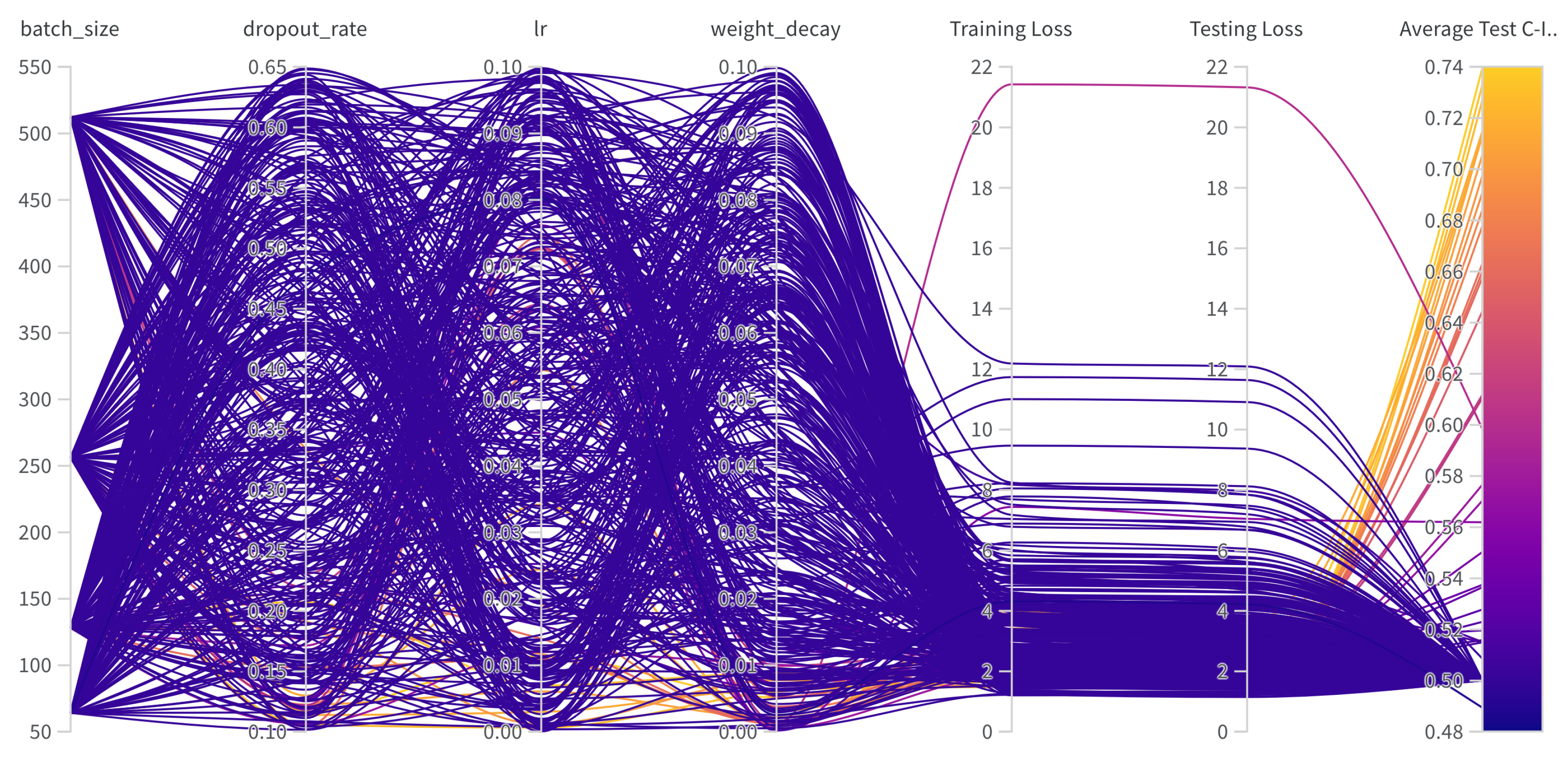

Table A1.
Hyperparameters search for training.
| Hyperparams | Training (range) |
|---|---|
| Learning Rate | [1e-6, 1e-1] |
| Weight Decay | [1e-6, 1e-1] |
| Dropout | [0.1, 0.65] |
| Batch Size | [64, 128, 256, 512] |
| Epochs | [50, 100] |
| Hidden Layers | [1, 2, 3, 4, 5, 6, 7, 8, 9] |
| Hidden Neurons | [2048, 1024, 512, 256, 128, 48, 32] |
| Optimizer | [adam, sgd, rmsprop, adamw] |
| Learning Rate Policy | [linear, exp, step, plateau, cosine] |
Appendix D. Frameworks, Compute Resources, and Wall-Clock Times
We trained SeNMo model using the Moffitt Cancer Center’s HPC machine using one Tesla V100 32GB GPU running Ubuntu 22.04.4 and CUDA 12.2. The entire code was developed in Python and PyTorch frameworks. The software frameworks and corresponding packages used in our codebase are given in Table A2. Training time for our current 83.33 Million parameter SeNMo encoder is approximately 11 hours. We conducted the hyperparameters search of the pan-cancer model for approximately 20 days using multiple GPUs in parallel. Finetuning the trained model on a given data having around 150 patients approximately takes 15 minutes.
Table A2.
Frameworks and packages used in our codebase.
| Package name | Version | |
|---|---|---|
| Operating systems | Ubuntu | 20.04.4 |
| Programming languages | Python | 3.10.13 |
| Deep learning framework | Pytorch | 2.2.0 |
| torchvision | 0.17.0 | |
| feature-engine | 1.6.2 | |
| imbalanced-learn | 0.12.0 | |
| Miscellaneous | scipy | 1.12.0 |
| scikit-learn | 1.4.0 | |
| numpy | 1.26.3 | |
| PyYaml | 6.0.1 | |
| jupyter | 1.0.0 | |
| pandas | 2.2.0 | |
| pickle5 | 0.0.11 | |
| protobuf | 4.25.2 | |
| wandb | 0.16.3 |
References
- Jiang, P.; Sinha, S.; Aldape, K.; Hannenhalli, S.; Sahinalp, C.; Ruppin, E. Big data in basic and translational cancer research. Nature Reviews Cancer 2022, 22, 625–639. [Google Scholar] [CrossRef]
- Hanahan, D.; Weinberg, R.A. Hallmarks of cancer: the next generation. cell 2011, 144, 646–674. [Google Scholar] [CrossRef] [PubMed]
- Acosta, J.N.; Falcone, G.J.; Rajpurkar, P.; Topol, E.J. Multimodal biomedical AI. Nature Medicine 2022, 28, 1773–1784. [Google Scholar] [CrossRef]
- Chatsirisupachai, K.; Lesluyes, T.; Paraoan, L.; Van Loo, P.; De Magalhães, J.P. An integrative analysis of the age-associated multi-omic landscape across cancers. Nature communications 2021, 12, 2345. [Google Scholar] [CrossRef]
- Qin, D. Next-generation sequencing and its clinical application. Cancer biology & medicine 2019, 16, 4. [Google Scholar]
- Waqas, A.; Tripathi, A.; Ramachandran, R.P.; Stewart, P.; Rasool, G. Multimodal data integration for oncology in the era of deep neural networks: a review. arXiv 2023, arXiv:2303.06471. [Google Scholar] [CrossRef] [PubMed]
- Chistyakov, D.V.; Guryleva, M.V.; Stepanova, E.S.; Makarenkova, L.M.; Ptitsyna, E.V.; Goriainov, S.V.; Nikolskaya, A.I.; Astakhova, A.A.; Klimenko, A.S.; Bezborodova, O.A.; et al. Multi-omics approach points to the importance of oxylipins metabolism in early-stage breast cancer. Cancers 2022, 14, 2041. [Google Scholar] [CrossRef] [PubMed]
- Ullah, I.; Yang, L.; Yin, F.T.; Sun, Y.; Li, X.H.; Li, J.; Wang, X.J. Multi-omics approaches in colorectal cancer screening and diagnosis, recent updates and future perspectives. Cancers 2022, 14, 5545. [Google Scholar] [CrossRef]
- Chen, Y.C.; Hsu, C.L.; Wang, H.M.; Wu, S.G.; Chang, Y.L.; Chen, J.S.; Wu, Y.C.; Lin, Y.T.; Yang, C.Y.; Lin, M.W.; et al. Multiomics Analysis Reveals Molecular Changes during Early Progression of Precancerous Lesions to Lung Adenocarcinoma in Never-Smokers. Cancer Research 2025, 85, 602–617. [Google Scholar] [CrossRef]
- Zhang, S.; Deshpande, A.; Verma, B.K.; Wang, H.; Mi, H.; Yuan, L.; Ho, W.J.; Jaffee, E.M.; Zhu, Q.; Anders, R.A.; et al. Integration of clinical trial spatial multiomics analysis and virtual clinical trials enables immunotherapy response prediction and biomarker discovery. Cancer Research 2024, 84, 2734–2748. [Google Scholar] [CrossRef]
- Underwood, T. Pan-cancer analysis of whole genomes. Nature 2020, 578, 82–93. [Google Scholar]
- Zgura, A.; Chipuc, S.; Bacalbasa, N.; Haineala, B.; Rodica, A.; Sebastian, V. Evaluating Tumour Mutational Burden as a Key Biomarker in Personalized Cancer Immunotherapy: A Pan-Cancer Systematic Review. Cancers 2025, 17, 480. [Google Scholar] [CrossRef] [PubMed]
- Divate, M.; Tyagi, A.; Richard, D.J.; Prasad, P.A.; Gowda, H.; Nagaraj, S.H. Deep learning-based pan-cancer classification model reveals tissue-of-origin specific gene expression signatures. Cancers 2022, 14, 1185. [Google Scholar] [CrossRef] [PubMed]
- Kwon, H.J.; Park, U.H.; Goh, C.J.; Park, D.; Lim, Y.G.; Lee, I.K.; Do, W.J.; Lee, K.J.; Kim, H.; Yun, S.Y.; et al. Enhancing lung cancer classification through integration of liquid biopsy multi-omics data with machine learning techniques. Cancers 2023, 15, 4556. [Google Scholar] [CrossRef] [PubMed]
- Ahmed, S.; Nielsen, I.E.; Tripathi, A.; Siddiqui, S.; Ramachandran, R.P.; Rasool, G. Transformers in time-series analysis: A tutorial. Circuits, Systems, and Signal Processing 2023, 42, 7433–7466. [Google Scholar] [CrossRef]
- Waqas, A.; Dera, D.; Rasool, G.; Bouaynaya, N.C.; Fathallah-Shaykh, H.M. Brain tumor segmentation and surveillance with deep artificial neural networks. Deep Learning for Biomedical Data Analysis: Techniques, Approaches, and Applications 2021, pp. 311–350.
- Ahmed, S.; Dera, D.; Hassan, S.U.; Bouaynaya, N.; Rasool, G. Failure detection in deep neural networks for medical imaging. Frontiers in Medical Technology 2022, 4, 919046. [Google Scholar] [CrossRef]
- Waqas, A.; Farooq, H.; Bouaynaya, N.C.; Rasool, G. Exploring robust architectures for deep artificial neural networks. Communications Engineering 2022, 1, 46. [Google Scholar] [CrossRef]
- Steyaert, S.; Pizurica, M.; Nagaraj, D.; Khandelwal, P.; Hernandez-Boussard, T.; Gentles, A.J.; Gevaert, O. Multimodal data fusion for cancer biomarker discovery with deep learning. Nature machine intelligence 2023, 5, 351–362. [Google Scholar] [CrossRef]
- Li, J.; Xu, Q.; Wu, M.; Huang, T.; Wang, Y. Pan-cancer classification based on self-normalizing neural networks and feature selection. Frontiers in Bioengineering and Biotechnology 2020, 8, 766. [Google Scholar] [CrossRef]
- Chen, R.J.; Lu, M.Y.; Williamson, D.F.; Chen, T.Y.; Lipkova, J.; Noor, Z.; Shaban, M.; Shady, M.; Williams, M.; Joo, B.; et al. Pan-cancer integrative histology-genomic analysis via multimodal deep learning. Cancer Cell 2022, 40, 865–878. [Google Scholar] [CrossRef]
- Poirion, O.B.; Jing, Z.; Chaudhary, K.; Huang, S.; Garmire, L.X. DeepProg: an ensemble of deep-learning and machine-learning models for prognosis prediction using multi-omics data. Genome medicine 2021, 13, 1–15. [Google Scholar] [CrossRef] [PubMed]
- Khadirnaikar, S.; Shukla, S.; Prasanna, S. Integration of pan-cancer multi-omics data for novel mixed subgroup identification using machine learning methods. Plos one 2023, 18, e0287176. [Google Scholar] [CrossRef]
- Ma, T.; Zhang, A. Integrate multi-omics data with biological interaction networks using Multi-view Factorization AutoEncoder (MAE). BMC genomics 2019, 20, 944. [Google Scholar] [CrossRef] [PubMed]
- Ellen, J.G.; Jacob, E.; Nikolaou, N.; Markuzon, N. Autoencoder-based multimodal prediction of non-small cell lung cancer survival. Scientific Reports 2023, 13, 15761. [Google Scholar] [CrossRef] [PubMed]
- Zhao, N.; Guo, M.; Wang, K.; Zhang, C.; Liu, X. Identification of pan-cancer prognostic biomarkers through integration of multi-omics data. Frontiers in Bioengineering and Biotechnology 2020, 8, 268. [Google Scholar] [CrossRef]
- Nikolaou, N.; Salazar, D.; RaviPrakash, H.; Goncalves, M.; Mulla, R.; Burlutskiy, N.; Markuzon, N.; Jacob, E. Quantifying the advantage of multimodal data fusion for survival prediction in cancer patients. bioRxiv 2024, pp. 2024–01.
- Rong, Z.; Liu, Z.; Song, J.; Cao, L.; Yu, Y.; Qiu, M.; Hou, Y. MCluster-VAEs: an end-to-end variational deep learning-based clustering method for subtype discovery using multi-omics data. Computers in Biology and Medicine 2022, 150, 106085. [Google Scholar] [CrossRef]
- Pan, L.; Liu, D.; Dou, Y.; Wang, L.; Feng, Z.; Rong, P.; Xu, L.; Peng, S. Multi-Head Attention Mechanism Learning for Cancer New Subtypes and Treatment Based on Cancer Multi-Omics Data. arXiv 2023, arXiv:2307.04075. [Google Scholar]
- Jia, W.; Sun, M.; Lian, J.; Hou, S. Feature dimensionality reduction: a review. Complex & Intelligent Systems 2022, 8, 2663–2693. [Google Scholar]
- Krawczuk, J.; ukaszuk, T. The feature selection bias problem in relation to high-dimensional gene data. Artificial intelligence in medicine 2016, 66, 63–71. [Google Scholar] [CrossRef]
- Yang, S.; Guo, X.; Yu, K.; Huang, X.; Jiang, T.; He, J.; Gu, L. Causal feature selection in the presence of sample selection bias. ACM Transactions on Intelligent Systems and Technology 2023, 14, 1–18. [Google Scholar] [CrossRef]
- Weinstein, J.N.; Collisson, E.A.; Mills, G.B.; Shaw, K.R.; Ozenberger, B.A.; Ellrott, K.; Shmulevich, I.; Sander, C.; Stuart, J.M. The cancer genome atlas pan-cancer analysis project. Nature genetics 2013, 45, 1113–1120. [Google Scholar] [CrossRef] [PubMed]
- Ellis, M.J.; Gillette, M.; Carr, S.A.; Paulovich, A.G.; Smith, R.D.; Rodland, K.K.; Townsend, R.R.; Kinsinger, C.; Mesri, M.; Rodriguez, H.; et al. Connecting Genomic Alterations to Cancer Biology with Proteomics: The NCI Clinical Proteomic Tumor Analysis Consortium. Cancer Discovery 2013, 3, 1108–1112. [Google Scholar] [CrossRef] [PubMed]
- Cui, H.; Wang, C.; Maan, H.; Pang, K.; Luo, F.; Duan, N.; Wang, B. scGPT: toward building a foundation model for single-cell multi-omics using generative AI. Nature Methods, 2024; 1–11. [Google Scholar]
- Zhu, W.; Chen, Y.; Nie, S.; Yang, H. SAMMS: Multi-modality Deep Learning with the Foundation Model for the Prediction of Cancer Patient Survival. In Proceedings of the 2023 IEEE International Conference on Bioinformatics and Biomedicine (BIBM). IEEE; 2023; pp. 3662–3668. [Google Scholar]
- Chen, J.; Hu, Z.; Sun, S.; Tan, Q.; Wang, Y.; Yu, Q.; Zong, L.; Hong, L.; Xiao, J.; Shen, T.; et al. Interpretable RNA foundation model from unannotated data for highly accurate RNA structure and function predictions. arXiv 2022, arXiv:2204.00300 2022. [Google Scholar]
- Wang, H.; Yang, Y.; Zhao, Z.; Gu, P.; Sapkota, N.; Chen, D.Z. Path-GPTOmic: A Balanced Multi-modal Learning Framework for Survival Outcome Prediction. arXiv 2024, arXiv:2403.11375 2024. [Google Scholar]
- Tripathi, A.; Waqas, A.; Venkatesan, K.; Yilmaz, Y.; Rasool, G. Building Flexible, Scalable, and Machine Learning-ready Multimodal Oncology Datasets. Sensors 2024, 24, 1634. [Google Scholar] [CrossRef]
- Goldman, M.; Craft, B.; Hastie, M.; Repečka, K.; McDade, F.; Kamath, A.; Banerjee, A.; Luo, Y.; Rogers, D.; Brooks, A.N.; et al. The UCSC Xena platform for public and private cancer genomics data visualization and interpretation. biorxiv 2018, p. 326470.
- Satpathy, S.; Krug, K.; Beltran, P.M.J.; Savage, S.R.; Petralia, F.; Kumar-Sinha, C.; Dou, Y.; Reva, B.; Kane, M.H.; Avanessian, S.C.; et al. A proteogenomic portrait of lung squamous cell carcinoma. Cell 2021, 184, 4348–4371. [Google Scholar] [CrossRef]
- Stewart, P.A.; Welsh, E.A.; Slebos, R.J.; Fang, B.; Izumi, V.; Chambers, M.; Zhang, G.; Cen, L.; Pettersson, F.; Zhang, Y.; et al. Proteogenomic landscape of squamous cell lung cancer. Nature communications 2019, 10, 3578. [Google Scholar] [CrossRef]
- Sarhadi, V.K.; Armengol, G. Molecular biomarkers in cancer. Biomolecules 2022, 12, 1021. [Google Scholar] [CrossRef]
- Li, Y.; Porta-Pardo, E.; Tokheim, C.; Bailey, M.H.; Yaron, T.M.; Stathias, V.; Geffen, Y.; Imbach, K.J.; Cao, S.; Anand, S.; et al. Pan-cancer proteogenomics connects oncogenic drivers to functional states. Cell 2023, 186, 3921–3944. [Google Scholar] [CrossRef]
- Chen, F.; Wendl, M.C.; Wyczalkowski, M.A.; Bailey, M.H.; Li, Y.; Ding, L. Moving pan-cancer studies from basic research toward the clinic. Nature cancer 2021, 2, 879–890. [Google Scholar] [CrossRef]
- Liao, J.; Chin, K.V. Logistic regression for disease classification using microarray data: model selection in a large p and small n case. Bioinformatics 2007, 23, 1945–1951. [Google Scholar] [CrossRef] [PubMed]
- Galli, S. Feature-engine: A Python package for feature engineering for machine learning. Journal of Open Source Software 2021, 6, 3642. [Google Scholar] [CrossRef]
- Bommert, A.; Welchowski, T.; Schmid, M.; Rahnenführer, J. Benchmark of filter methods for feature selection in high-dimensional gene expression survival data. Briefings in Bioinformatics 2022, 23, bbab354. [Google Scholar] [CrossRef] [PubMed]
- Pedregosa, F.; Varoquaux, G.; Gramfort, A.; Michel, V.; Thirion, B.; Grisel, O.; Blondel, M.; Prettenhofer, P.; Weiss, R.; Dubourg, V.; et al. Scikit-learn: Machine Learning in Python. Journal of Machine Learning Research 2011, 12, 2825–2830. [Google Scholar]
- Anggraeny, F.T.; Purbasari, I.Y.; Munir, M.S.; Muttaqin, F.; Mandyarta, E.P.; Akbar, F.A. Analysis of Simple Data Imputation in Disease Dataset. In Proceedings of the International Conference on Science and Technology (ICST 2018). Atlantis Press; 2018; pp. 471–475. [Google Scholar]
- Ulriksborg, T.R. Imputation of missing time series values using statistical and mathematical strategies. Department of Informatics 2022. [Google Scholar]
- Yi, J.; Lee, J.; Kim, K.J.; Hwang, S.J.; Yang, E. Why not to use zero imputation? correcting sparsity bias in training neural networks. arXiv 2019, arXiv:1906.00150 2019. [Google Scholar]
- Chen, R.J.; Lu, M.Y.; Wang, J.; Williamson, D.F.; Rodig, S.J.; Lindeman, N.I.; Mahmood, F. Pathomic fusion: an integrated framework for fusing histopathology and genomic features for cancer diagnosis and prognosis. IEEE Transactions on Medical Imaging 2020, 41, 757–770. [Google Scholar] [CrossRef]
- Carreras, J.; Roncador, G.; Hamoudi, R. Artificial intelligence predicted overall survival and classified mature B-cell neoplasms based on immuno-oncology and immune checkpoint panels. Cancers 2022, 14, 5318. [Google Scholar] [CrossRef]
- Zhao, Z.; Zobolas, J.; Zucknick, M.; Aittokallio, T. Tutorial on survival modeling with applications to omics data. Bioinformatics 2024, btae132. [Google Scholar] [CrossRef]
- Miller, K.D.; Nogueira, L.; Mariotto, A.B.; Rowland, J.H.; Yabroff, K.R.; Alfano, C.M.; Jemal, A.; Kramer, J.L.; Siegel, R.L. Cancer treatment and survivorship statistics, 2019. CA: a cancer journal for clinicians 2019, 69, 363–385. [Google Scholar] [CrossRef]
- van Rijthoven, M.; Obahor, S.; Pagliarulo, F.; van den Broek, M.; Schraml, P.; Moch, H.; van der Laak, J.; Ciompi, F.; Silina, K. Multi-resolution deep learning characterizes tertiary lymphoid structures and their prognostic relevance in solid tumors. Communications Medicine 2024, 4, 5. [Google Scholar] [CrossRef] [PubMed]
- Chen, Z.; Wang, X.; Jin, Z.; Li, B.; Jiang, D.; Wang, Y.; Jiang, M.; Zhang, D.; Yuan, P.; Zhao, Y.; et al. Deep learning on tertiary lymphoid structures in hematoxylin-eosin predicts cancer prognosis and immunotherapy response. NPJ Precision Oncology 2024, 8, 73. [Google Scholar] [CrossRef] [PubMed]
- Klambauer, G.; Unterthiner, T.; Mayr, A.; Hochreiter, S. Self-normalizing neural networks. Advances in neural information processing systems 2017, 30. [Google Scholar]
- Li, Z.; Jiang, Y.; Lu, M.; Li, R.; Xia, Y. Survival prediction via hierarchical multimodal co-attention transformer: A computational histology-radiology solution. IEEE Transactions on Medical Imaging 2023. [Google Scholar] [CrossRef] [PubMed]
- Liu, Z.; Wang, Y.; Vaidya, S.; Ruehle, F.; Halverson, J.; Soljačić, M.; Hou, T.Y.; Tegmark, M. Kan: Kolmogorov-arnold networks. arXiv 2024, arXiv:2404.19756 2024. [Google Scholar]
- Gore, S.; Azad, R.K. CancerNet: a unified deep learning network for pan-cancer diagnostics. BMC bioinformatics 2022, 23, 229. [Google Scholar] [CrossRef]
- Loyfer, N.; Magenheim, J.; Peretz, A.; Cann, G.; Bredno, J.; Klochendler, A.; Fox-Fisher, I.; Shabi-Porat, S.; Hecht, M.; Pelet, T.; et al. A DNA methylation atlas of normal human cell types. Nature 2023, 613, 355–364. [Google Scholar] [CrossRef]
- Lakshminarasimhan, R.; Liang, G. The role of DNA methylation in cancer. DNA Methyltransferases-Role and Function 2016, pp. 151–172.
- Du, P.; Zhang, X.; Huang, C.C.; Jafari, N.; Kibbe, W.A.; Hou, L.; Lin, S.M. Comparison of Beta-value and M-value methods for quantifying methylation levels by microarray analysis. BMC bioinformatics 2010, 11, 1–9. [Google Scholar] [CrossRef]
- Wang, Z.; Wu, X.; Wang, Y. A framework for analyzing DNA methylation data from Illumina Infinium HumanMethylation450 BeadChip. BMC bioinformatics 2018, 19, 15–22. [Google Scholar] [CrossRef]
- Corchete, L.A.; Rojas, E.A.; Alonso-López, D.; De Las Rivas, J.; Gutiérrez, N.C.; Burguillo, F.J. Systematic comparison and assessment of RNA-seq procedures for gene expression quantitative analysis. Scientific reports 2020, 10, 19737. [Google Scholar] [CrossRef]
- Hijazo-Pechero, S.; Alay, A.; Marín, R.; Vilariño, N.; Muñoz-Pinedo, C.; Villanueva, A.; Santamaría, D.; Nadal, E.; Solé, X. Gene expression profiling as a potential tool for precision oncology in non-small cell lung cancer. Cancers 2021, 13, 4734. [Google Scholar] [CrossRef] [PubMed]
- Gonzalez, A.; Leon, D.A.; Perera, Y.; Perez, R. On the gene expression landscape of cancer. Plos one 2023, 18, e0277786. [Google Scholar] [CrossRef] [PubMed]
- Rau, A.; Flister, M.; Rui, H.; Auer, P.L. Exploring drivers of gene expression in the Cancer Genome Atlas. Bioinformatics 2019, 35, 62–68. [Google Scholar] [CrossRef] [PubMed]
- Expression, G. Expression atlas, 2024. Available online: https://www.ebi.ac.uk.
- Peng, Y.; Croce, C.M. The role of MicroRNAs in human cancer. Signal transduction and targeted therapy 2016, 1, 1–9. [Google Scholar] [CrossRef]
- Chu, A.; Robertson, G.; Brooks, D.; Mungall, A.J.; Birol, I.; Coope, R.; Ma, Y.; Jones, S.; Marra, M.A. Large-scale profiling of microRNAs for the cancer genome atlas. Nucleic acids research 2016, 44, e3–e3. [Google Scholar] [CrossRef]
- Lin, S.; Zhou, J.; Xiao, Y.; Neary, B.; Teng, Y.; Qiu, P. Integrative analysis of TCGA data identifies miRNAs as drug-specific survival biomarkers. Scientific Reports 2022, 12, 6785. [Google Scholar] [CrossRef]
- Documentation, G. Reverse Phase Protein Array. Available online: https://docs.gdc.cancer.gov/Data/Bioinformatics_Pipelines/RPPA_intro/ (accessed on 13 May 2024).
- Anderson, M. RPPA Description. 2024. Available online: https://www.mdanderson.org/documents/core-facilities/Functional Proteomics RPPA Core Facility/RPPA Description2016.pdf (accessed on 13 May 2024).
- Chen, M.J.M.; Li, J.; Wang, Y.; Akbani, R.; Lu, Y.; Mills, G.B.; Liang, H. TCPA v3. 0: an integrative platform to explore the pan-cancer analysis of functional proteomic data. Molecular & Cellular Proteomics 2019, 18, S15–S25. [Google Scholar]
- Li, J.; Lu, Y.; Akbani, R.; Ju, Z.; Roebuck, P.L.; Liu, W.; Yang, J.Y.; Broom, B.M.; Verhaak, R.G.; Kane, D.W.; et al. TCPA: a resource for cancer functional proteomics data. Nature methods 2013, 10, 1046–1047. [Google Scholar] [CrossRef]
- Ju, Z.; Liu, W.; Roebuck, P.L.; Siwak, D.R.; Zhang, N.; Lu, Y.; Davies, M.A.; Akbani, R.; Weinstein, J.N.; Mills, G.B.; et al. Development of a robust classifier for quality control of reverse-phase protein arrays. Bioinformatics 2015, 31, 912–918. [Google Scholar] [CrossRef]
- Commons, G.D. Mutation Annotation Format. 2024. Available online: https://docs.gdc.cancer.gov/Encyclopedia/pages/Mutation_Annotation_Format/ (accessed on 13 May 2024).
- Commons, G.D. File Format - VCF. 2024. Available online: https://docs.gdc.cancer.gov/Data/File_Formats/VCF_Format/ (accessed on 13 May 2024).
- Commons, G.D. File Format - MAF. 2024. Available online: https://docs.gdc.cancer.gov/Data/File_Formats/MAF_Format/ (accessed on 13 May 2024).
- Mendiratta, G.; Ke, E.; Aziz, M.; Liarakos, D.; Tong, M.; Stites, E.C. Cancer gene mutation frequencies for the US population. Nature communications 2021, 12, 5961. [Google Scholar] [CrossRef]
- Morin, O.; Vallières, M.; Braunstein, S.; Ginart, J.B.; Upadhaya, T.; Woodruff, H.C.; Zwanenburg, A.; Chatterjee, A.; Villanueva-Meyer, J.E.; Valdes, G.; et al. An artificial intelligence framework integrating longitudinal electronic health records with real-world data enables continuous pan-cancer prognostication. Nature Cancer 2021, 2, 709–722. [Google Scholar] [CrossRef] [PubMed]
- Lewandowska, A.; Rudzki, G.; Lewandowski, T.; Stryjkowska-Gora, A.; Rudzki, S. Risk factors for the diagnosis of colorectal cancer. Cancer Control 2022, 29, 10732748211056692. [Google Scholar] [CrossRef] [PubMed]
- Lopes-Ramos, C.M.; Quackenbush, J.; DeMeo, D.L. Genome-wide sex and gender differences in cancer. Frontiers in oncology 2020, 10, 597788. [Google Scholar] [CrossRef]
- Zavala, V.A.; Bracci, P.M.; Carethers, J.M.; Carvajal-Carmona, L.; Coggins, N.B.; Cruz-Correa, M.R.; Davis, M.; de Smith, A.J.; Dutil, J.; Figueiredo, J.C.; et al. Cancer health disparities in racial/ethnic minorities in the United States. British journal of cancer 2021, 124, 315–332. [Google Scholar] [CrossRef]
- Yang, X.; Mu, D.; Peng, H.; Li, H.; Wang, Y.; Wang, P.; Wang, Y.; Han, S. Research and application of artificial intelligence based on electronic health records of patients with cancer: systematic review. JMIR Medical Informatics 2022, 10, e33799. [Google Scholar] [CrossRef]
- Ching, T. Cox regression. 2024. Available online: http://traversc.github.io/cox-nnet/docs/ (accessed on 13 May 2024).
- Davidson-Pilon, C. lifelines, survival analysis in Python. [CrossRef]
- Documentation, P. HuberLoss. 2024. Available online: https://pytorch.org/docs/stable/generated/torch.nn.HuberLoss.html (accessed on 13 May 2024).
- Biewald, L. Experiment Tracking with Weights and Biases. Software available from wandb.com. 2020. Available online: https://www.wandb.com/.
Figure 1.
Overview of the SeNMo model. The data from public sources are collected using MINDS [39] and curated to develop the multimodal dataset for SeNMo training. MINDS is a metadata framework for fusing publicly available data sources like TCGA-GDC and UCSC Xena Portal into machine learning-ready format [33,39,40]. The dataset is preprocessed and fed to the self-normalizing deep learning encoder network that learns underlying sub-visual patterns from cross-modality, pan-cancer data. The learned encoder weights are later used for different downstream tasks (with or without fine-tuning), such as predicting the overall survival (OS), progression-free survival (PFS), cancer subtype classification, grading, or tertiary lymph structures (TLS) ratio.
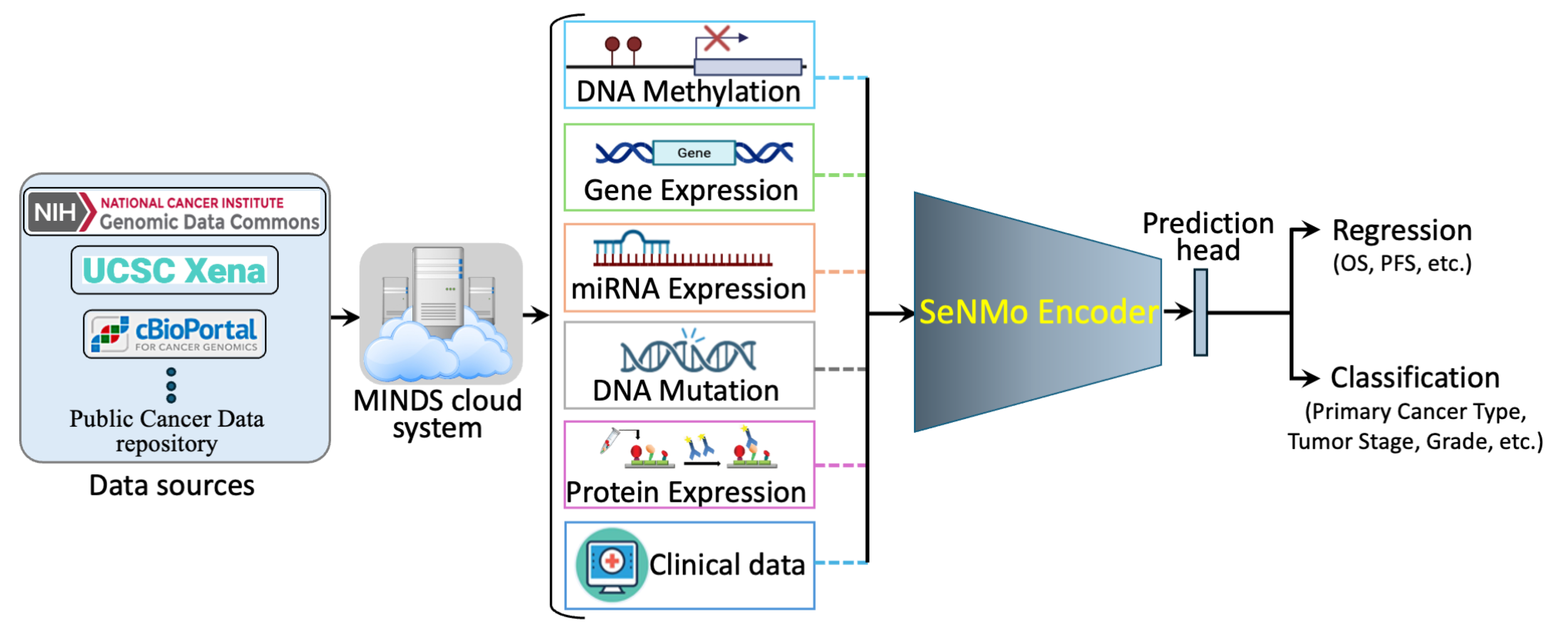
Figure 2.
Features processing pipeline for pan-cancer data encompassing six data types: DNA Methylation, Gene Expression, miRNA Expression, Protein Expression, DNA Mutation, and Clinical features. Initial feature counts are reduced through preprocessing, with each modality unified at the pan-cancer level to yield unimodal pan-cancer feature sets. These unimodal features are further unified across all modalities, resulting in a final integrated multimodal feature matrix of 80,697 features, used for downstream analysis.
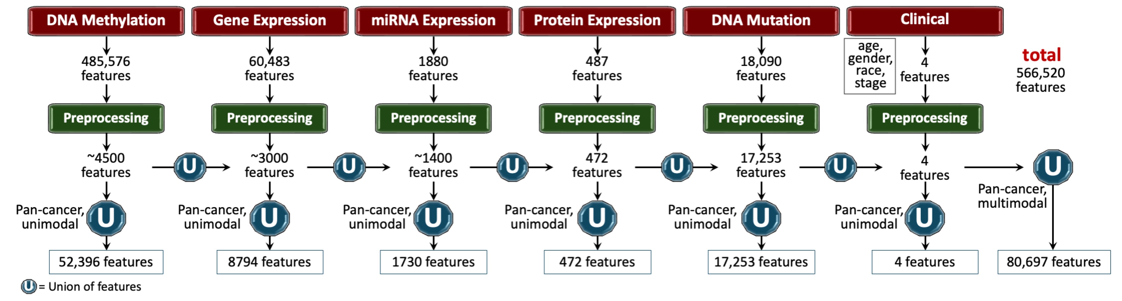
Figure 3.
Summary of the survival data and number of cases in the pan-cancer data. The top panel illustrates patient survival in years, with each line representing an individual patient, marked as censored or dead, and grouped by cancer type. The bottom panel displays the number of cases for each primary cancer type, highlighting variation in sample sizes across cancers, which range from high counts in breast, kidney, and lung to lower counts in rare cancers like diffuse large B-cell lymphoma.
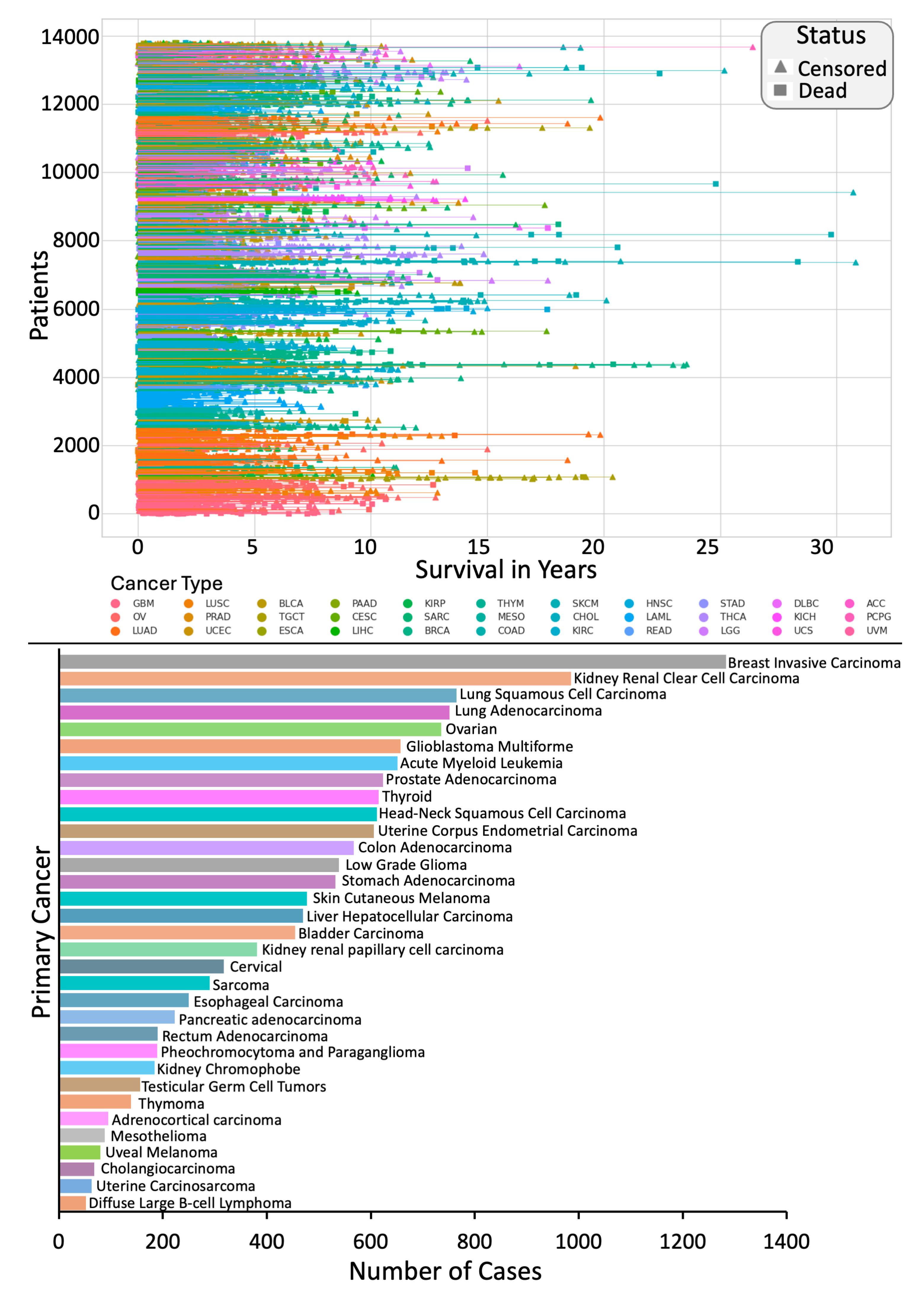
Figure 4.
Study design and simulations for SeNMo across different learning regimes, datasets, and tasks. The baseline model (row 1) is first trained on TCGA data with 33 cancer types for overall survival (OS) prediction. Rows 2–5 represent variations: red-bordered boxes indicate a change from the baseline (e.g., out-of-distribution task and/or data), while green-bordered boxes align with the baseline. Simulations include OS prediction on both seen and unseen data (rows 2 and 3) and new tasks such as primary cancer type classification and TLS ratio prediction on seen and unseen datasets (rows 4 and 5).
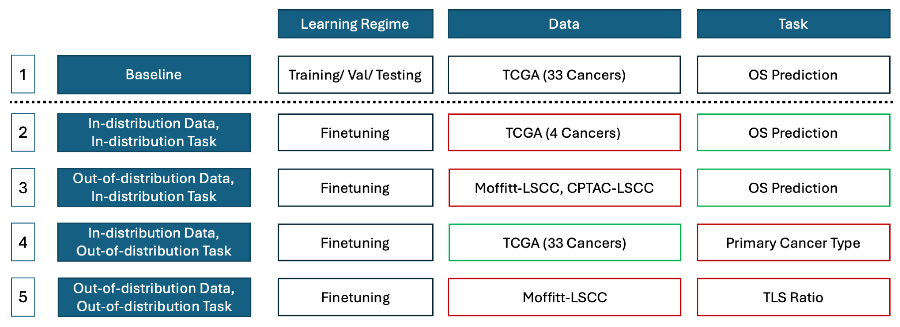
Figure 5.
Pan-cancer C-Index results for OS prediction. The SeNMo model was trained and evaluated using different combinations of data modalities. Training and validation were carried out on the of the total data, whereas inference was done on the held-out test set. As the number of modalities increased in the pan-cancer data, the model’s performance improved, as depicted by the upward trend of C-Index. All the results shown here are statistically significant, i.e., .
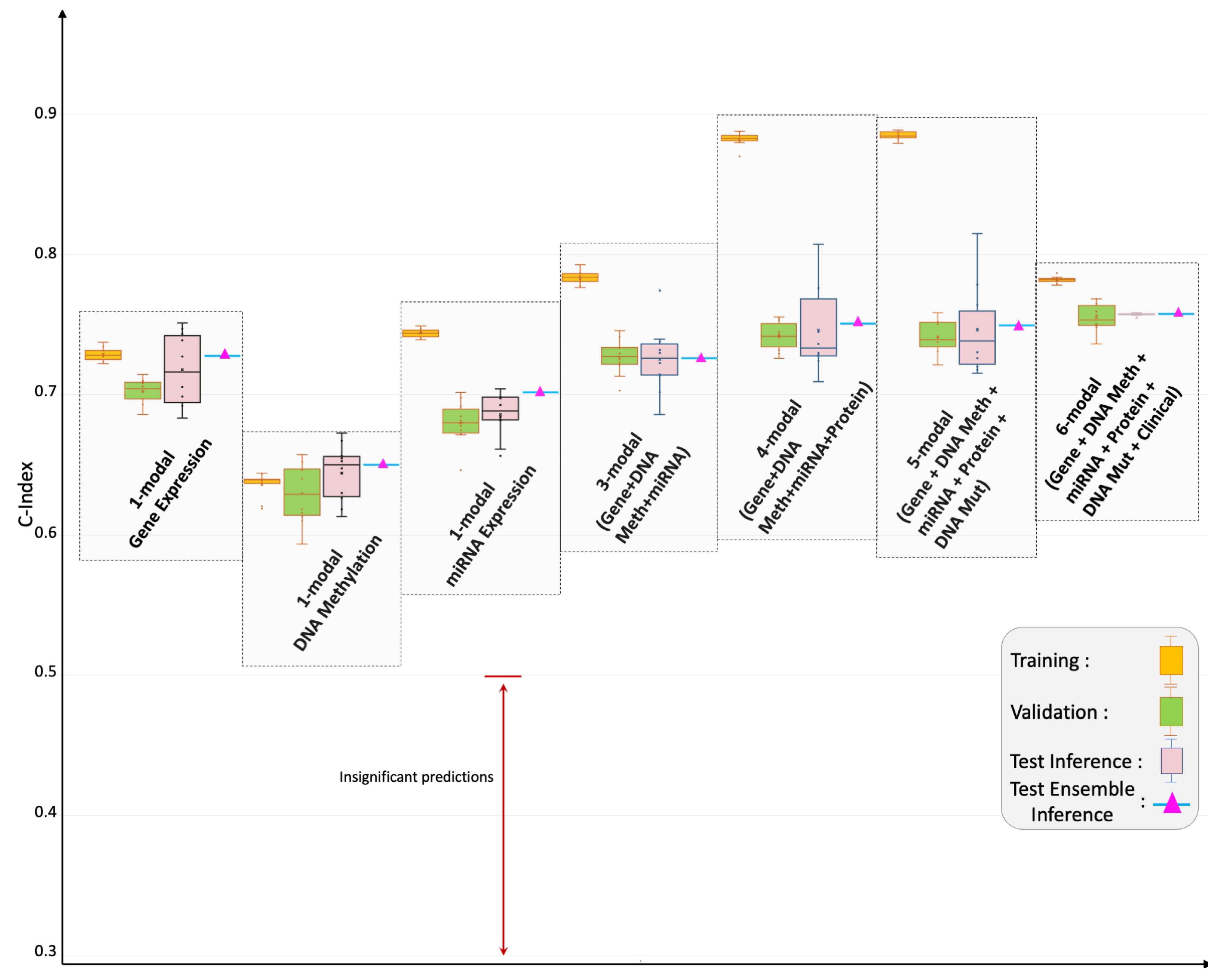
Figure 6.
Cancer-specific C-index results for overall survival (OS) prediction across multiple cancer types. Pink box plots represent predictions on the held-out test set, while green box plots show predictions from fine-tuned models for cancer types with initially insignificant results or for unseen data, such as Moffitt LSCC and CPTAC-LSCC. Triangular markers indicate ensemble predictions, with blue triangles representing fine-tuned ensemble results. Models with insignificant predictions fall below the 0.5 threshold, marked by a red arrow. Although trained on pan-cancer cohort, SeNMo effectively captures survival times across individual cancers, with fine-tuning improving performance for cases with initially low predictive significance.
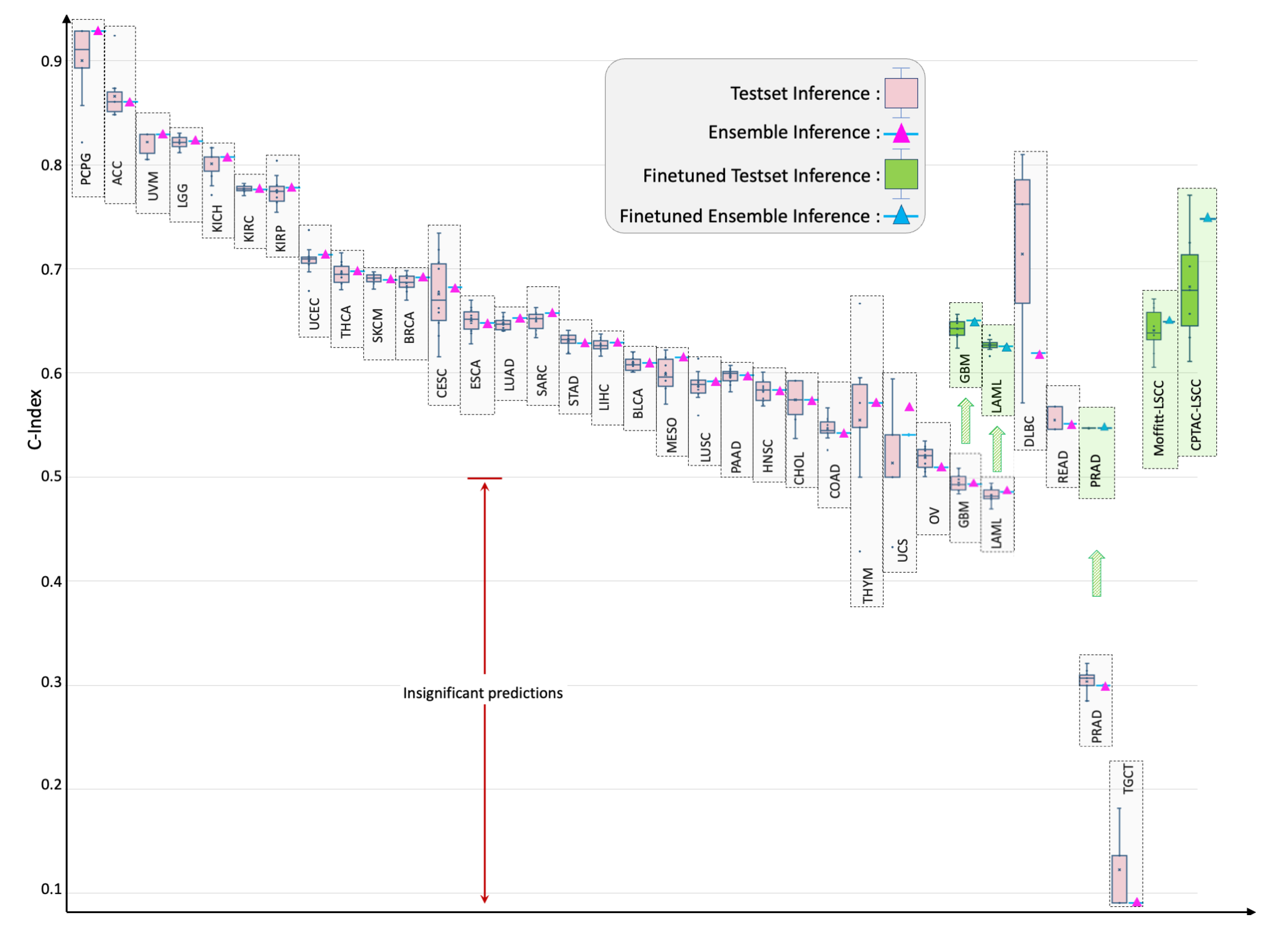
Figure 7.
Kaplan-Meier (KM) comparative analysis of using SeNMo in stratifying patient outcomes in low/ intermediate/ high risk, defined by the 33-66-100 percentile of hazard predictions. Hazard predictions from SeNMo show clear distinctions between stratified groups. The p-values from logrank test for Low vs. Intermediate: , Low vs. High: , and Intermediate vs. High: . The shaded areas around each curve depicts the 95% confidence intervals.
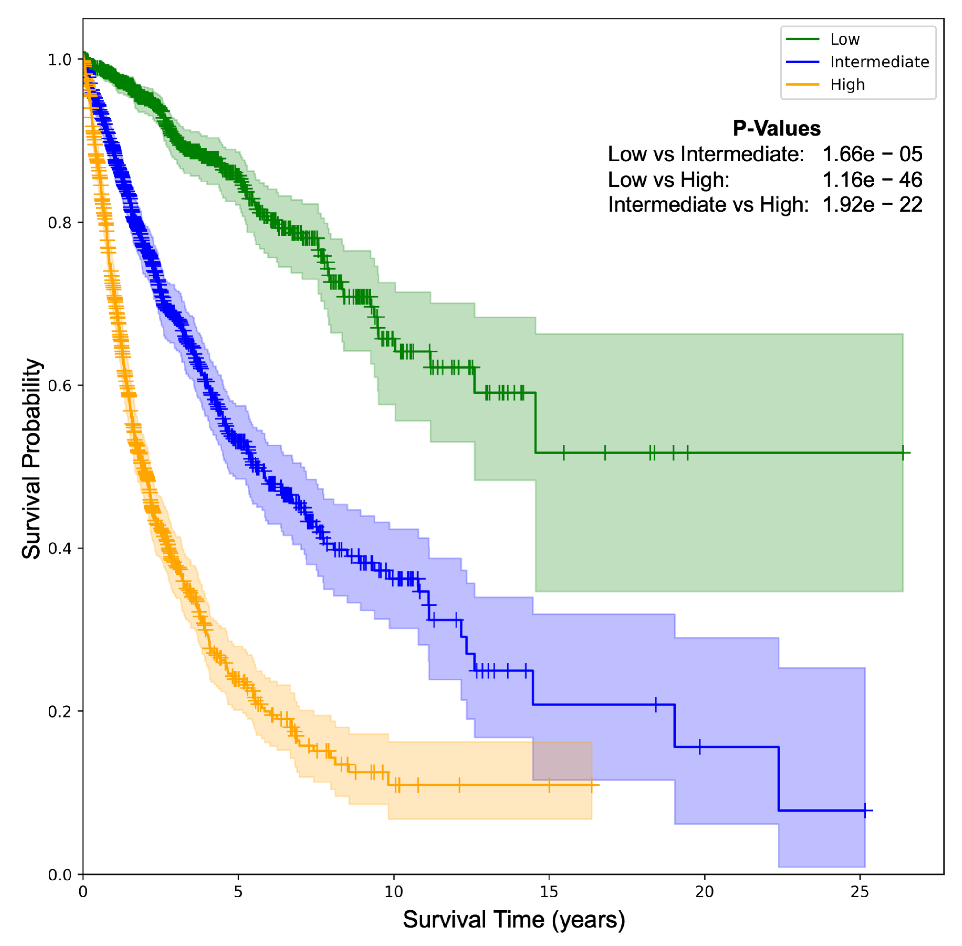
Figure 8.
Pan-cancer primary cancer type prediction results. The model’s accuracy across training, validation, and inference stages is near-perfect (top left panel). Confusion matrix (bottom left) shows minimal misclassifications, while the scatter plot (bottom middle) shows the alignment of predicted versus true labels. The classification report (right panel) shows high precision, recall, and f1-scores in the 33 cancers type-identification.
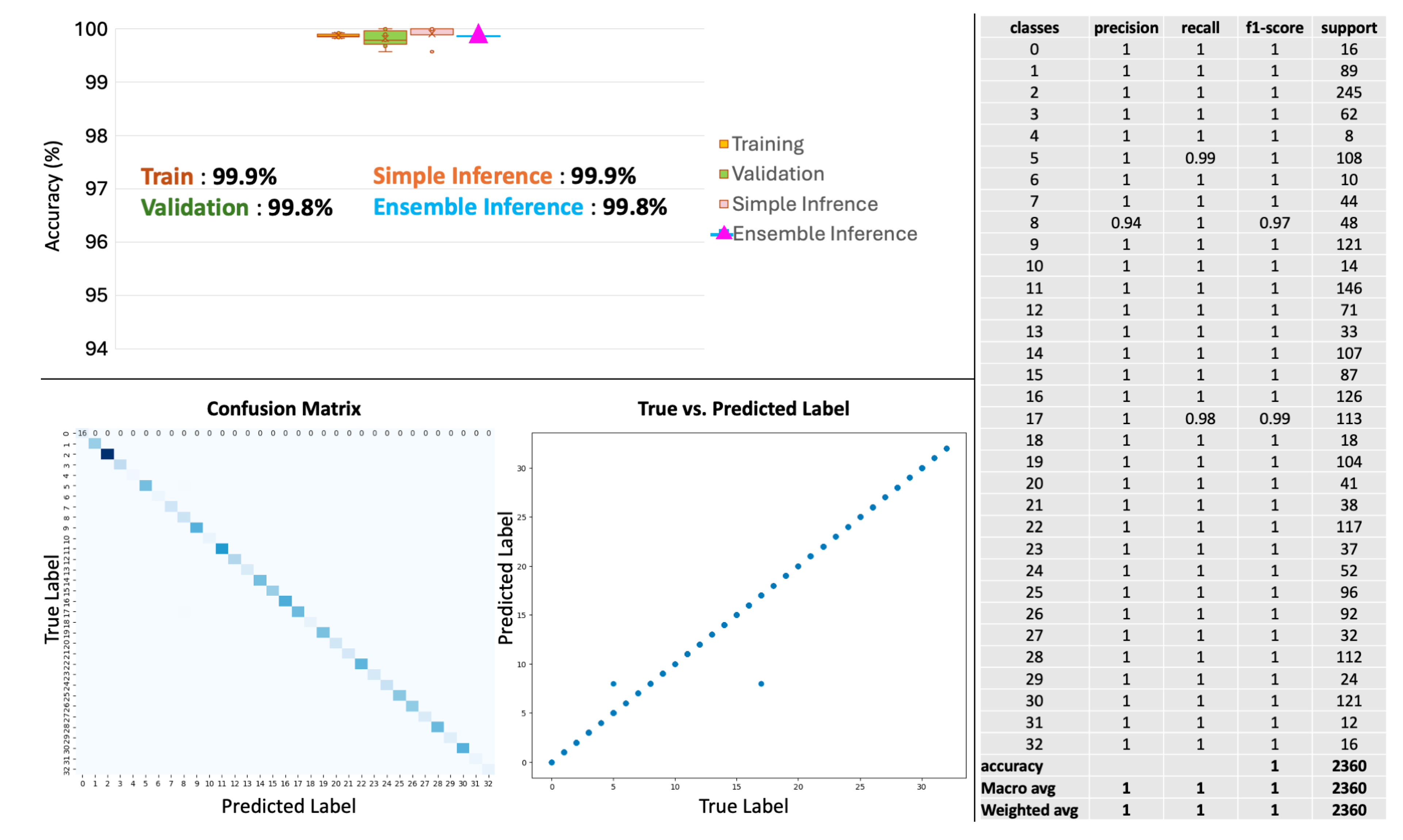
Figure 9.
Tertiary Lymph Structures (TLS) Ratio Predictions by SeNMo. (a) Dataset distribution, dividing 103 samples into training, validation, test, and excluding those missing TLS data. (b) Box plots compare TLS ratios between manual annotations (M) and SeNMo predictions, showing no significant difference (). (c) Violin plot of TLS Ratio annotations for high vs. low groups thresholded by the median value, with a significant difference (). (d) Violin plot of SeNMo’s TLS Ratio predictions, also showing significant separation between high and low groups (). (e) Kaplan-Meier survival curves with significant survival differences, comparing high vs. low TLS ratios for both annotations (top, ) and SeNMo predictions (bottom, ).
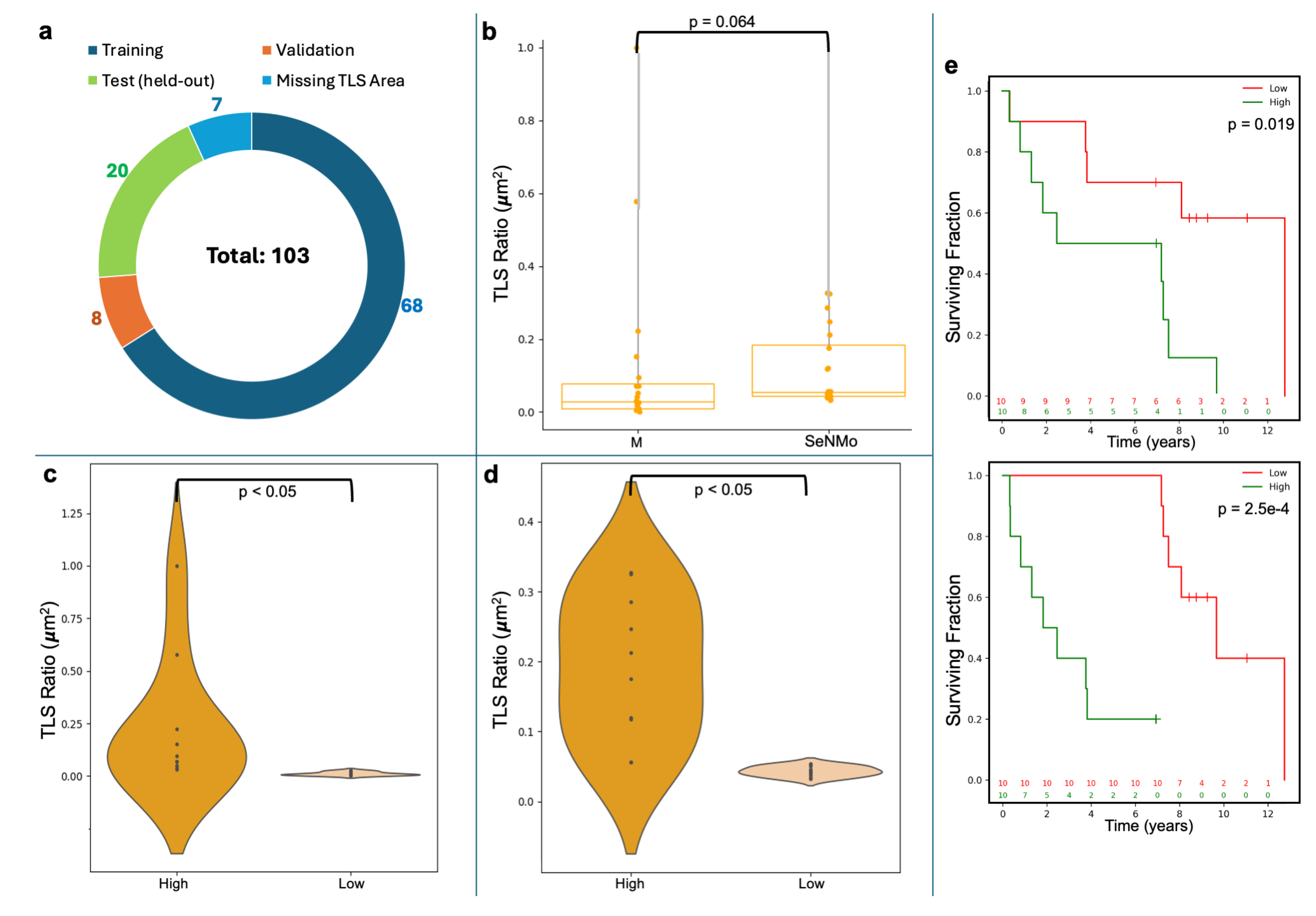
Table 1.
Feature Reduction Summary of Pan-cancer data.
| Data (TCGA-GDC) | Primary Site | Cases | miRNA Exprn | DNA Methyl | Gene Exprn | Protein Exprn | DNA Mut | |||||
|---|---|---|---|---|---|---|---|---|---|---|---|---|
| Before | After | Before | After | Before | After | Before | After | Before | After | |||
| TCGA-DLBC | Large B-cell Lymphoma | 51 | 1880 | 1060 | 485576 | 4396 | 60483 | 850 | 487 | 472 | 18090 | 17253 |
| TCGA-UCS | Uterine Carcinosarcoma | 61 | 1880 | 1101 | 485576 | 4632 | 60483 | 1231 | 487 | 472 | 18090 | 17253 |
| TCGA-CHOL | Bile Duct | 62 | 1880 | 967 | 485576 | 4479 | 60483 | 1261 | 487 | 472 | 18090 | 17253 |
| TCGA-UVM | Uveal melanomas | 80 | 1880 | 1162 | 485576 | 4019 | 60483 | 772 | 487 | 472 | 18090 | 17253 |
| TCGA-MESO | Mesothelioma | 86 | 1880 | 1158 | 485576 | 4372 | 60483 | 1278 | 487 | 472 | 18090 | 17253 |
| TCGA-ACC | Adrenocortical | 95 | 1880 | 1110 | 485576 | 4454 | 60483 | 1304 | 487 | 472 | 18090 | 17253 |
| TCGA-THYM | Thymoma | 138 | 1880 | 1245 | 485576 | 4609 | 60483 | 1337 | 487 | 472 | 18090 | 17253 |
| TCGA-TGCT | Testicular | 139 | 1880 | 1290 | 485576 | 4762 | 60483 | 1343 | 487 | 472 | 18090 | 17253 |
| TCGA-READ | Rectal | 178 | 1880 | 1314 | 485576 | 4077 | 60483 | 1547 | 487 | 472 | 18090 | 17253 |
| TCGA-KICH | Kidney Chromophobe | 182 | 1880 | 1089 | 485576 | 4333 | 60483 | 1107 | 487 | 472 | 18090 | 17253 |
| TCGA-PCPG | Pheochromocytoma and Paraganglioma | 189 | 1880 | 1251 | 485576 | 4550 | 60483 | 1216 | 487 | 472 | 18090 | 17253 |
| TCGA-PAAD | Pancreatic | 222 | 1880 | 1308 | 485576 | 4518 | 60483 | 1567 | 487 | 472 | 18090 | 17253 |
| TCGA-ESCA | Esophageal | 249 | 1880 | 1300 | 485576 | 4192 | 60483 | 1684 | 487 | 472 | 18090 | 17253 |
| TCGA-SARC | Sarcoma | 287 | 1880 | 1235 | 485576 | 4467 | 60483 | 2490 | 487 | 472 | 18090 | 17253 |
| TCGA-CESC | Cervical | 304 | 1880 | 1405 | 485576 | 4167 | 60483 | 2017 | 487 | 472 | 18090 | 17253 |
| TCGA-KIRP | Kidney Papillary Cell Carcinoma | 376 | 1880 | 1297 | 485576 | 4078 | 60483 | 1798 | 487 | 472 | 18090 | 17253 |
| TCGA-SKCM | Skin Cutaneous Melanoma | 436 | 1880 | 1426 | 485576 | 4427 | 60483 | 2488 | 487 | 472 | 18090 | 17253 |
| TCGA-BLCA | Bladder | 447 | 1880 | 1361 | 485576 | 4483 | 60483 | 2751 | 487 | 472 | 18090 | 17253 |
| TCGA-LIHC | Liver | 463 | 1880 | 1336 | 485576 | 4023 | 60483 | 2017 | 487 | 472 | 18090 | 17253 |
| TCGA-STAD | Stomach | 499 | 1880 | 1397 | 485576 | 4196 | 60483 | 2354 | 487 | 472 | 18090 | 17253 |
| TCGA-LGG | Lower Grade Glioma | 533 | 1880 | 1287 | 485576 | 4193 | 60483 | 1560 | 487 | 472 | 18090 | 17253 |
| TCGA-COAD | Colon | 539 | 1880 | 1460 | 485576 | 4671 | 60483 | 1931 | 487 | 472 | 18090 | 17253 |
| TCGA-UCEC | Endometrioid | 588 | 1880 | 1414 | 485576 | 4424 | 60483 | 2849 | 487 | 472 | 18090 | 17253 |
| TCGA-HNSC | Head and Neck | 611 | 1880 | 1428 | 485576 | 4358 | 60483 | 2059 | 487 | 472 | 18090 | 17253 |
| TCGA-THCA | Thyroid | 614 | 1880 | 1369 | 485576 | 4160 | 60483 | 1432 | 487 | 472 | 18090 | 17253 |
| TCGA-PRAD | Prostate | 623 | 1880 | 1334 | 485576 | 4006 | 60483 | 1635 | 487 | 472 | 18090 | 17253 |
| TCGA-LAML | Acute Myeloid Leukemia | 626 | 1880 | 1140 | 485576 | 4415 | 60483 | 1032 | 487 | 472 | 18090 | 17253 |
| TCGA-GBM | Glioblastoma | 649 | 1880 | 1023 | 485576 | 4076 | 60483 | 1206 | 487 | 472 | 18090 | 17253 |
| TCGA-LUAD | Lung Adenocarcinoma | 728 | 1880 | 1360 | 485576 | 4480 | 60483 | 2562 | 487 | 472 | 18090 | 17253 |
| TCGA-OV | Ovarian | 731 | 1880 | 1430 | 485576 | 4254 | 60483 | 2116 | 487 | 472 | 18090 | 17253 |
| TCGA-LUSC | Lung Squamous Cell Carcinoma | 752 | 1880 | 1375 | 485576 | 4302 | 60483 | 2610 | 487 | 472 | 18090 | 17253 |
| TCGA-KIRC | Kidney Clear Cell Carcinoma | 979 | 1880 | 1333 | 485576 | 4399 | 60483 | 2274 | 487 | 472 | 18090 | 17253 |
| TCGA-BRCA | Breast | 1260 | 1880 | 1418 | 485576 | 4195 | 60483 | 3671 | 487 | 472 | 18090 | 17253 |
Table 2.
Summary of patient characteristics for pan-cancer data in this study.
| Cancer Type | Age (Mean ± SD) |
Gender (M/F) |
Race (White/Asian/Black/NA/ American Indian/Alaska) |
Stage (0/I/IA/IB/IC/II/IIA/IIB/IIC/III/ IIIA/IIIB/IIIC/IV/IVA/IVB/IVC/NA) |
|---|---|---|---|---|
| TCGA-ACC | 47.46 ± 16.20 | 33/62 | 79/3/1/12/0 | 0/9/0/0/0/46/0/0/0/20/0/0/0/17/0/0/0/3 |
| TCGA-BLCA | 67.92 ± 10.39 | 326/121 | 363/43/23/18/0 | 0/3/0/0/0/136/0/0/0/159/0/0/0/148/0/0/0/1 |
| TCGA-BRCA | 57.94 ± 13.11 | 13/1247 | 915/59/198/87/1 | 0/114/94/7/0/6/404/307/0/2/176/30/74/22/0/0/0/24 |
| TCGA-CESC | 48.04 ± 13.70 | 0/304 | 211/19/32/30/9 | 0/0/0/0/0/0/0/0/0/0/0/0/0/0/0/0/0/304 |
| TCGA-CHOL | 64.37 ± 12.21 | 30/32 | 55/3/3/1/0 | 0/30/0/0/0/16/0/0/0/5/0/0/0/2/3/6/0/0 |
| TCGA-COAD | 66.93 ± 12.67 | 288/251 | 261/11/67/198/2 | 0/87/1/0/0/46/150/13/2/26/9/69/47/56/18/3/0/12 |
| TCGA-DLBC | 56.76 ± 13.68 | 24/27 | 32/18/1/0/0 | 0/0/0/0/0/0/0/0/0/0/0/0/0/0/0/0/0/51 |
| TCGA-ESCA | 64.22 ± 12.11 | 208/41 | 162/46/6/35/0 | 0/14/9/7/0/1/56/43/0/41/16/10/9/7/6/0/0/30 |
| TCGA-GBM | 57.74 ± 14.32 | 399/250 | 547/13/53/36/0 | 0/0/0/0/0/0/0/0/0/0/0/0/0/0/0/0/0/649 |
| TCGA-HNSC | 61.02 ± 11.92 | 443/168 | 522/12/58/17/2 | 0/29/0/0/0/93/0/0/0/97/0/0/0/0/302/13/1/76 |
| TCGA-KICH | 51.61 ± 14.12 | 99/83 | 154/6/19/3/0 | 0/75/0/0/0/59/0/0/0/34/0/0/0/14/0/0/0/0 |
| TCGA-KIRC | 60.67 ± 11.95 | 641/338 | 876/16/73/14/0 | 0/475/0/0/0/102/0/0/0/237/0/0/0/161/0/0/0/4 |
| TCGA-KIRP | 61.98 ± 12.20 | 278/98 | 275/6/75/16/4 | 0/219/0/0/0/25/0/0/0/77/0/0/0/21/0/0/0/34 |
| TCGA-LAML | 54.82 ± 15.87 | 345/281 | 564/8/49/5/0 | 0/0/0/0/0/0/0/0/0/0/0/0/0/0/0/0/626 |
| TCGA-LGG | 42.71 ± 13.32 | 293/240 | 492/8/22/10/1 | 0/0/0/0/0/0/0/0/0/0/0/0/0/0/0/0/533 |
| TCGA-LIHC | 60.44 ± 13.71 | 305/158 | 255/168/25/14/1 | 0/211/0/0/0/105/0/0/0/6/78/12/11/2/1/3/0/34 |
| TCGA-LUAD | 65.20 ± 10.08 | 329/399 | 580/14/84/48/2 | 0/7/194/195/0/2/67/103/0/0/101/12/0/37/0/0/0/10 |
| TCGA-LUSC | 67.28 ± 8.62 | 548/204 | 530/12/47/163/0 | 0/4/127/243/0/4/87/138/0/3/94/33/0/12/0/0/0/7 |
| TCGA-MESO | 63.01 ± 9.78 | 70/16 | 84/1/1/0/0 | 0/7/2/1/0/15/0/0/0/45/0/0/0/16/0/0/0/0 |
| TCGA-OV | 59.60 ± 11.44 | 0/731 | 626/25/43/33/3 | 0/0/0/0/0/0/0/0/0/0/0/0/0/0/0/0/731 |
| TCGA-PAAD | 64.87 ± 11.36 | 123/99 | 195/13/8/6/0 | 0/1/6/15/0/0/36/148/0/6/0/0/0/7/0/0/0/3 |
| TCGA-PCPG | 47.02 ± 15.15 | 84/105 | 157/7/20/4/1 | 0/0/0/0/0/0/0/0/0/0/0/0/0/0/0/0/189 |
| TCGA-PRAD | 60.93 ± 6.80 | 623/0 | 510/13/81/18/1 | 0/0/0/0/0/0/0/0/0/0/0/0/0/0/0/0/623 |
| TCGA-READ | 63.83 ± 11.85 | 98/80 | 90/1/7/80/0 | 0/37/0/0/0/7/40/2/1/6/7/25/14/21/7/0/0/11 |
| TCGA-SARC | 60.70 ± 14.38 | 129/158 | 253/5/20/9/0 | 0/0/0/0/0/0/0/0/0/0/0/0/0/0/0/0/287 |
| TCGA-SKCM | 57.84 ± 15.41 | 289/174 | 441/12/1/9/0 | 6/30/18/30/0/39/18/28/61/44/16/46/68/23/0/0/0/36 |
| TCGA-STAD | 65.44 ± 10.53 | 320/179 | 311/108/15/64/0 | 0/1/21/46/0/37/54/71/0/4/88/67/39/47/0/0/0/24 |
| TCGA-TGCT | 31.87 ± 9.19 | 139/0 | 124/4/6/5/0 | 0/69/26/11/0/4/6/1/1/2/1/6/5/0/0/0/0/7 |
| TCGA-THCA | 47.17 ± 15.83 | 166/448 | 413/59/35/106/1 | 0/350/0/0/0/64/0/0/0/134/0/0/0/4/52/0/8/2 |
| TCGA-THYM | 58.12 ± 13.00 | 72/66 | 115/13/8/2/0 | 0/0/0/0/0/0/0/0/0/0/0/0/0/0/0/0/138 |
| TCGA-UCEC | 63.74 ± 11.06 | 0/588 | 402/21/120/32/4 | 0/0/0/0/0/0/0/0/0/0/0/0/0/0/0/0/588 |
| TCGA-UCS | 70.07 ± 9.24 | 0/61 | 50/1/9/1/0 | 0/0/0/0/0/0/0/0/0/0/0/0/0/0/0/0/61 |
| TCGA-UVM | 61.65 ± 13.95 | 45/35 | 55/0/0/25/0 | 0/0/0/0/0/0/12/27/0/0/25/10/1/4/0/0/0/1 |
| Moffitt-LSCC | 69.14 ± 8.34 | 72/36 | 105/0/3/0/0 | 0/0/24/25/0/0/31/15/0/0/12/1/0/0/0/0/0/0 |
Table 3.
C-Index for Test and Ensemble Inference across Cancer Types.
| Cancer Type | C-Index {Test, Ensemble} |
Cancer Type | C-Index {Test, Ensemble} |
|---|---|---|---|
| TCGA-PCPG | {0.900, 0.929} | TCGA-DLBC | {0.714, 0.619} |
| TCGA-ACC | {0.866, 0.861} | TCGA-MESO | {0.599, 0.615} |
| TCGA-UVM | {0.822, 0.829} | TCGA-LUSC | {0.588, 0.592} |
| TCGA-LGG | {0.821, 0.823} | TCGA-PAAD | {0.597, 0.598} |
| TCGA-KICH | {0.801, 0.807} | TCGA-HNSC | {0.583, 0.583} |
| TCGA-KIRC | {0.777, 0.776} | TCGA-CHOL | {0.574, 0.574} |
| TCGA-KIRP | {0.775, 0.778} | TCGA-COAD | {0.546, 0.542} |
| TCGA-UCEC | {0.708, 0.713} | TCGA-THYM | {0.555, 0.571} |
| TCGA-THCA | {0.696, 0.698} | TCGA-UCS | {0.514, 0.541} |
| TCGA-SKCM | {0.691, 0.689} | TCGA-OV | {0.518, 0.509} |
| TCGA-BRCA | {0.687, 0.692} | TCGA-READ | {0.550, 0.551} |
| TCGA-CESC | {0.676, 0.682} | TCGA-GBM | {0.495, 0.493}* |
| TCGA-ESCA | {0.650, 0.648} | TCGA-GBM (finetuning) | {0.642, 0.650} |
| TCGA-LUAD | {0.647, 0.653} | TCGA-LAML | {0.482, 0.485}* |
| TCGA-SARC | {0.650, 0.658} | TCGA-LAML (finetuning) | {0.627, 0.626} |
| TCGA-STAD | {0.631, 0.628} | TCGA-PRAD | {0.304, 0.300}* |
| TCGA-LIHC | {0.627, 0.629} | TCGA-PRAD (finetuning) | {0.541, 0.542}* |
| TCGA-BLCA | {0.609, 0.609} | TCGA-TGCT | {0.123, 0.091}* |
* not statistically significant ()
Disclaimer/Publisher’s Note: The statements, opinions and data contained in all publications are solely those of the individual author(s) and contributor(s) and not of MDPI and/or the editor(s). MDPI and/or the editor(s) disclaim responsibility for any injury to people or property resulting from any ideas, methods, instructions or products referred to in the content. |
© 2025 by the authors. Licensee MDPI, Basel, Switzerland. This article is an open access article distributed under the terms and conditions of the Creative Commons Attribution (CC BY) license (http://creativecommons.org/licenses/by/4.0/).
Copyright: This open access article is published under a Creative Commons CC BY 4.0 license, which permit the free download, distribution, and reuse, provided that the author and preprint are cited in any reuse.


