
Submitted:
04 April 2025
Posted:
07 April 2025
Read the latest preprint version here
Abstract
The mean-field model (MFM) is the workhorse of the statistical mechanics: one normally accepts that it yields results which, despite differing numerically from the correct ones, are not “very wrong”, in that they resemble the actual behavior of the system as eventually obtained by a more advanced treatments. This, for example, turns out to be the case for the Casimir force under, say, Dirichlet-Dirichlet, (+,+) and (+,−) boundary conditions (BC) for which, according to the general expectations the MFM delivers attractive for like BC—or repulsive for unlike BC—force, with the principally correct position of the maximum strength of the force below, or above the critical point Tc. It turns out, however, that this is not the case with Dirichlet-Neumann (DN) BC. In this case, the mean-field approach leads to an attractive Casimir force. This contradiction with the “boundary condition rule” is cured in the case of the Gaussian model under DN BC. Our results, which are mathematically exact, demonstrate that the Casimir force within the MFM is attractive as a function of temperature T and external magnetic field h, while for the Gaussian model it is repulsive for h=0, and can be, surprisingly, both repulsive and attractive for h≠0. The treatment of the MFM is based on the exact solution of one non-homogeneous nonlinear differential equation of second order. The Gaussian model is analyzed both in its continuum and lattice realization. The obtained outcome teaches us that the mean-field results should be accepted with caution in the case of fluctuation-induced forces and ought to be checked against more precise treatment of the fluctuations within the envisaged system.
Keywords:
finite-size effects
; exact results
; Casimir force
; mean-field model
; Gaussian model
; phase transitions
; critical phenomena
; phase diagrams
1. Introduction
Currently, the most prominent example of a fluctuation-induced force is the force due to quantum or thermal fluctuations of the electromagnetic field, leading to the so-called QED Casimir effect, named after the Dutch physicist H.B. Casimir who first realized that in the case of two perfectly-conducting, uncharged, and smooth plates parallel to each other in vacuum, at these fluctuations lead to an attractive force between them [1]. Thirty years after Casimir, Fisher and De Gennes [2] showed that a very similar effect exists in critical fluids, today known as critical Casimir effect. A summary of the results available for this effect can be found in the recent reviews [3,4,5,6]. The description of the critical Casimir effect is based on finite-size scaling theory [7,8,9]. Let us envisage a system with a film geometry , , and with boundary conditions imposed along the spatial direction of finite extent L. Take to be the total free energy of such a system within the grand canonical ensemble (GCE). Then, if is the free energy per area A of the system, one can define the Casimir force for critical systems in the grand-canonical -ensemble, see, e.g. Refs. [4,9,10,11]::
where
is the so-called excess (over the bulk) free energy per area and per . Here we suppose a system at temperature T is exposed to an external ordering field h, which couples linearly to its order parameter—such as the number density, the concentration difference, the magnetization etc. Actually, the thermodynamic Casimir force per area is the excess pressure over the bulk one due to the finite size of that system:
Here is the pressure in the finite system under boundary conditions , while is the one in the infinite, i.e., macroscopically large, system. The above definition is actually equivalent to Eq. (1.1). Note that is the excess grand potential per area, is the grand canonical potential per area of the finite system, while has the meaning of the grand potential per volume V for the macroscopically large system. The equivalence between the definitions in Eqs. (1.1) and (1.3) stems from the observation that for the finite system one has , while for the bulk one and .
When the excess pressure is inward towards the system, i.e., there is an attraction of the surfaces of the system towards each other and a repulsion if .
2. The Casimir Force Within the Continuum Gaussian Model
The continuum version of the Gaussian model with a scalar order parameter consists of the linear and bilinear terms in the Ginzburg-Landau-Wilson formulation of a system in d dimensions that undergoes a continuous symmetry-breaking phase transition at low temperatures. The partition function of this system is the functional integral
where
In (2.2) t is the reduced temperature, proportional to , and h is the spatially constant ordering field. Because of the Gaussian nature of the free energy functional the partition function resolves into the product
where is the partition function of the system with . The geometry of the system under consideration is a slab of large—ultimately infinite—cross section and finite thickness L.
With regard to scaling considerations, there are two combinations of parameters that reflect the predictions of finite size scaling. They are
where , the correlation length exponent, is equal to 1/2 in the Gaussian model, and as noted above d is the dimensionality of the system. Our end results for the Casimir forces acting upon the systems will depend on the boundary conditions imposed. In all cases, the form of the Casimir force is
All results reported in this portion of the article rely on two results, which can be obtained with the use of contour integration techniques; see also [12]. The two results are
In order to carry out the evaluation of the free energy of the Gaussian model we turn to the basis set of functions that will be used to construct the free energy with and without an ordering field. These functions allow us to evaluate the partition function by integrating over the amplitudes of the contributions of each member of the set to the order parameter. Here, we focus on the case of periodic boundary conditions. Ignoring the dependence on position in the “plane” of the slab, the functions are the orthonormal set
with n a positive integer. It is straightforward to show that this set is orthonormal as a function of z in that
The three function types are all mutually orthogonal. In the case of higher dimensions, we construct a new basis set by multiplying the functions (2.9)–(2.11) by suitable functions of the orthogonal position variables. Those functions can be taken to be of the form , where is a -dimensional position vector in the plane of the slab and is in its reciprocal space.
We then express the order parameter as follows
The free energy for a given configuration of the Gaussian order parameter, in terms of the amplitudes in the expansion of the order parameter in the basis set (2.12)–(2.14), is
The last term in brackets above reflects the fact that the only basis function that the constant external field couples to is the constant function in (2.11)
The next step is to exponentiate the expression in (2.16), multiply by either , or setting , by -1, and, after that, to perform the Gaussian integrals over the ’s, the ’s, and . The resulting partition function is given by
The coefficient A in (2.17) is the dimensional area of the slab.
As our next step we evaluate the sum over n on the right hand side of the expression for the partition function. To achieve this, we take the t-derivative of the logarithm of the summand, perform the sum over n and then integrate the resulting expression with respect to t. Taking the derivative of the summand in (2.17) with respect to t leaves us with the sum
which follows from (2.7). This integrates up to
The large-L limit of (2.19) is
To find the contribution to the Casimir force per unit area, we take the L-derivative of the difference between (2.20) and (2.19) and then integrate over . The derivative yields
The sum over values of is expressible as an integral, which takes the form
where, to get to the last line of (2.22) we defined a new integration variable and then made use of the definition (2.4) of . The implication of (2.22) is that we can express the contribution to the Casimir force as times a function of the scaling temperature variable . The coefficient in the equations above is the geometric factor
In the case of three dimensions, further processing of the result (2.22) is possible. We find
where is the polylogarithm function; see [13]. A plot of the function is shown in Figure 1.
The first term in parentheses in Eq. (2.17) gives us the h-dependent contribution to the free energy: . This is to be compared to the corresponding free energy of a neighboring bulk phase, which goes as , where is an extent that will ultimately be taken to go to infinity. If you add the two free energies, the dependence on L, the thickness of the slab, disappears. This means that there is no h-dependent free energy when slab boundary conditions are periodic, and hence no h-dependent contribution to the Casimir force.
The calculations in the case of periodic boundary conditions point the way to evaluating the partition function and the Casimir force of the case of Dirichlet-Neumann boundary conditions.
In this case the (unnormalized) basis functions are, exclusive of their dependence on the in-plane coordinates,
Examples of these functions are shown in Figure 2. Focusing on the h-independent contribution to the partition function, the sum to perform in this case is (see (2.28))
Note that in the limit of large L the right hand side goes to the expected asymptotic form. If we subtract that limiting form, and integrate with respect to t, we are left with
Finally, we take minus the derivative of this with respect to L, leaving us with
Making use of the analysis of previous sections, this leaves us with the following result for the Casimir force in the case of the d-dimensional Gaussian model with Dirichlet-Neumann boundary conditions
When , we have
Figure 3 shows what the function looks like when .
In order to find the h-dependent contribution to the Casimir force we turn to the normalized the basis set in the case of Dirichlet-Neumann boundary conditions. Assuming that the boundary conditions are Dirichlet at and Neumann at , this basis set is
with n an integer and
It is straightforward to establish that
while
As it turns out there is no need to take into account any dependence of the basis set on coordinates in the plane of the slab. This is because a constant ordering field couples only to order parameter configurations that are independent of those coordinates.
With this in mind, we expand the order parameter as follows
The Gaussian integrations over the ’s leaves us with the summation over n for the h-dependent contribution to the partition function
where the evaluation of the sum over n in (2.36) is accomplished with the use of (2.8) and a partial fraction decomposition of the summand. The first term in parentheses on the last line of (2.36) gives us exactly the same expression as the h-dependent contribution to the partition function of the slab with periodic boundary conditions. Its influence on the Casimir force is exactly canceled by the influence of the bulk. What remains is
where we have made use of the definition of the scaling combination in (2.5). The scaling form of the contribution to the Casimir force is, then
This function is shown in Figure 4. Note that this function is aways attractive.
The total scaling function is given by
Figure 5 shows what this function looks like.
Another depiction of the scaling contribution to the Casimir force for Dirichlet-Neumann boundary conditions in the three dimensional Gaussian model with a scalar order paremeter, , Figure 6, highlights the regions in which the function is attractive and repulsive.
3. The Casimir Force Within the Lattice Gaussian Model
We consider a ferromagnetic model with nearest-neighbor interactions on a fully finite d-dimensional hypercubic lattice of sites. Let us take to be the parallelepiped , where × denotes the direct (Cartesian) product of the finite sets .
It is convenient to consider the configuration space as an Euclidean vector space in which each configuration is represented by a column-vector with components labeled according to the lexicographic order of the set . Let be the corresponding transposed row-vector and let the dot (·) denote matrix multiplication. Then, for given boundary conditions , specified for each pair of opposite faces of by some takes the form
Here , where J is the interaction constant (to be set to in the remainder), and the interaction matrix can be written as
where is the one-dimentional discrete Laplacian defined on the finite chain under boundary conditions , and is the unit matrix.
By using the results of [9], we can write down the eigenfunctions of the interaction matrix (3.2) in the form
and obtain the corresponding eigenvalues of it
Obviously, . Note that the interaction Hamiltonian (3.1) has negative eigenvalues, which makes necessary the inclusion of a positive-definite quadratic form in the Gibbs exponent, to ensure the existence of the corresponding partition function. Thus, we consider the Hamiltonian
Here is a column-vector representing (in units of ) the inhomogeneous magnetic field configuration acting upon the system, and let be the transposed row-vector.
In order to ensure the existence of the partition function, all the eigenvalues , , of the quadratic form in , ought to be positive. Hence, the field must satisfy the inequality
with
defining the critical temperature of the finite system. Since, as stated above , it is clear that for the infinite system
The free energy density of a finite system in a region is
In Eq. (3.9) the first two terms do not depend on the size of the system, i.e., they are the same in both finite and infinite systems. The other two terms do depend, however on the size of the system. The function is due to the spin-spin interaction (and will be called "interaction term"); it depends on s, but does not depend on h. It is equal to
and is obtained after performing the corresponding Gaussian integrals in the free energy of the finite system. The dependence of the free energy on the field variables h is given by the "field term"
Here denotes the projection of the magnetic field configuration on the eigenfunction ( by we denote the complex conjugate of ):
Defining so, that
the above expressions can be rewritten in the form
and
Using the notations of [9], below we give a list of the complete sets of orthonormal eigenfunctions, , , of the one-dimensional discrete Laplacian under the Neumann - Dirichlet (ND) boundary conditions:
- periodic (p) boundary conditions
- Neumann - Dirichlet (ND) boundary conditions
The quantities , , are defined as follows
Now we are ready to find the finite-size behavior of the Gaussian model under the Dirichlet-Neumann boundary conditions. According to Eq. (3.17), , i.e., one has there realization of Neumann boundary conditions, while , which corresponds to Dirichlet boundary conditions. Thus, in the envisaged one-dimensional chain one has L independent spin variables .
We start with the consideration of dimensional system. Note that:
- under fully periodic (p) boundary conditions, , one has , hence .
- under Neumann-Dirichlet boundary conditions along z direction, i.e., , one has , hence .
3.1. The Gaussian Model on a Lattice for the Case
The behavior of the interaction term
We set and use the short-hand notation for these boundary conditions. Then, we perform in Eq. (3.10) the limits , keeping fixed. For the interaction term one then obtains
where
The behavior of the interaction term in the bulk system
In accord with Eq. (3.20), one has
The behavior of the interaction term in the film system with Neumann-Dirichlet boundary conditions
Explicitly, from Eq. (3.19) one obtains
with
This sum is of the form
where is defined as
The summations in Eq. (3.24) can be performed using [12] the identity
With the help of the identity one derives
Obviously . Thus, the part of the excess free energy under Neumann – Dirichlet boundary conditions that depends only on the interaction term is
Thus, can be decomposed in the sum of and where
and
Let us consider the behavior of and in the scaling regime
Let us first start with the function . Obviously, if then will be exponentially small. Thus, we need to consider the regime . It follows that . From Eq. (3.25) we obtain
It follows that
where we have introduced polar coordinates. In terms of them becomes
where R can be defined from the constraint , i.e., .
Next, we deal with . Taking into account that is small we derive
Note that for one has that for the L-dependent part of one has , i.e., is one order of magnitude smaller that . Because of that, contributes only sub-leading contributions to L-dependent part of the excess free energy and, therefore, to the Casimir force. Based on the above, we will no longer be interested in the function .
Summarizing the above, we conclude that the excess free energy can be written in a scaling form
where is a non-universal constants, and is an universal scaling function, , where T has the meaning of the temperature of the system, and is its bulk temperature. From Eq. (3.34), taking into account that with one has , we identify that
The behavior of the field term
The dependence of the free energy on the field variable is given by the "field term", given by Eq. (3.15). For a homogeneous filed h and for and boundary conditions, it is easy to obtain that
-
for boundary conditionsandObviously
- for boundary conditions
Thus, setting and , for a film geometry we arrive at
It is easy to show that
Thus, one has
Let us consider the small k behavior of the above sum. One derives
In the limits and for the behavior of the field term one obtains
When , then , we obtain that
which indeed equals the bulk expression - see Eq. (3.40).
From Eq. (3.45) for the behavior of the susceptibility in the finite system we derive
According to the finite-size scaling theory [9,15]
where and are non-universal constants, and is an universal scaling function, , where T has the meaning of the temperature of the system, and is its bulk temperature. From Eq. (3.48), taking into account that , we identify that
It is clear that the field term in the free energy of the finite system will be of the same order as the field term, i.e., if . In order to achieve that, we define a field dependent scaling variable
In terms of it, Eq. (3.45) becomes
The behavior of the scaling function is given in Figure 7.
Then for the excess free energy related to the field term, see Eq. (3.9), one derives
3.2. The Behavior of the Casimir Force
Let us determine the contributions of the interaction term and of the field term . Obviously, one has
We start with determining the behavior of . By definition, it is equal to
From Eq. (3.28) we derive the exact expression
Here we did not make any assumption bout L. Naturally, we will obtain a scaling form of only for . Then Eq. (3.32) is valid and, after performing the integration, we arrive at
where
The behavior of the scaling function is given in Figure 8. Obviously, the function is positive, which means that the Casimir force is repulsive when the external field is zero. For the Casimir amplitude we obtain
Obviously, Eq. (3.59) coincides with the corresponding result for the Gaussian model obtained via studying the , model — see [4, Eq.(6.99)]. Analogically, after proper renaming of the scaling variable the expression Eq. (3.58) of the scaling function of the force coinsides with the corresponding one for the , model — see [4, Eq.(6.104)].
Let us now determine the h-dependent part of the Casimir force. By definition, one has
Then, from Eq. (3.53) one obtains
where
A visualization of as a function of y for is shown in Figure 9.
The total Casimir force is a sum of , see Eq. (3.58), and given by Eq. (3.63). The plot of the result as a function of for is shown in Figure 10. As we see, the force can be both positive and negative, i.e., repulsive and attractive.
The overall behavior of the force as a function both on and is given in Figure 11.
4. The Casimir Force Within the Mean-Field Model
We start by defining the mean-field model used in the current study.
4.1. The Ginzburg-Landau Functional
In the present work we consider the standard Ginzburg–Landau functional
with
Here , while , and are the independent and dependent variables, respectively, and the prime indicates differentiation with respect to the variable z.
The functional (4.1) describes a critical system of Ising type in a film geometry , where the film thickness L is supposed to be along the z axis. In Equation (4.1), is the order parameter of the system, which is assumed to depend on the perpendicular position only, g is the bare coupling constant, and, as before, is the bare reduced temperature and h is the external ordering field. Given , h and L, the physical state of the regarded system is described by the minimizer of the respective Ginzburg–Landau functional given above whose extremals are determined by the solutions of the corresponding Euler-Lagrange equation
In case the Lagrangian density is defined by Equation (4.2), Equation (4.3) reads
Multiplying Equation (4.4) by and integrating once over z one obtains that
is a first integral of Equation (4.4), cf., e.g., [4,16,17]. This means that P is a constant on any smooth solution of the Euler-Lagrange equation (4.4).
In general, the thermodynamic Casimir force in such a system is the excess pressure, over the bulk one, acting on the boundaries of the finite system, which is due to the finite size of that system, i.e.,
Here is the pressure in the finite system, while is that one in the infinite system.
Now, assuming that the thickness L of the film is free to move, the variation of the free energy of the finite system is given as follows
(see, e.g., [18, p. 54], [19, p. 260] and [20]), where and are the variations of the independent and dependent variables, while
is the one-dimensional counterpart of the stress tensor (see, e.g., [21,22]). Relation (4.7) estimates the change of the finite-size contribution to the free energy of the system corresponding to a small variation of the variables including the variation of the film thickness L. In this sense, can be interpreted (see, e.g., [17,23]) as the pressure in the finite system, that is
On the other hand, taking into account Equations (4.2) and (4.8), one can see that
and hence is a constant on any smooth solution of the Euler-Lagrange equation (4.4) including the minimizer of the Ginzburg–Landau functional (4.1). Thus, the pressure in the finite system is
where is the foregoing minimizer.
As for the bulk system, it is easy to see following the same way of reasoning that the corresponding pressure is
Here, the value of the order parameter of the bulk system is determined as the constant solution of Equation (4.4), i.e., as the root of the cubic equation
that minimizes
Of course, does not depend on the boundary conditions at all. Let us note that , i.e., has its maximum over the solution of the cubic equation for (4.13).
Obviously, the relation (4.11) does not depend on the boundary conditions applied on the finite system too. This dependence arises solely from the dependency of the order parameter profile that minimizes the particular boundary value problem considered.
In the light of the above it is evident that once the order parameter profile and its bulk value are known in analytic form for given values of the parameters and h, then the respective Casimir force is determined in an exact manner by Equation (4.6).
In the current article we consider the Dirichlet-Neumann boundary conditions meaning that
In addition, is a critical exponent characterizing the behavior of the correlation length, while is another exponent related to the behavior of, say, order parameter as a function of the external field h.
It is convenient to introduce new parameters
and variables
where and , while and are the respective amplitudes of the correlation length along the and h axes (see, e.g., [22,24,25]). In terms of these new parameters and variables, Equations (4.1), (4.2), (4.4) and (4.5) becomes
and
respectively. The primes here and hereafter indicate differentiation with respect to the variable . Then, according to Equations (4.6), (4.11) and (4.12), the expression for the Casimir force written by means of the new parameters (4.16) and variables (4.17) reads
where and are the minimizers of the functional (4.18) and its “bulk counterpart” corresponding to and .
As mentioned above, in the present article we assume that the system is subject to Dirichlet-Neumann boundary conditions, that is
In other words, we are interested in the solution of Equation (4.20) that meet the conditions (4.23). It should be remarked that exact results associated with the Casimir effect have been derived in Refs. [17,23,26,27,28,29,30] in the cases of , and Dirichlet-Dirichlet boundary conditions.
4.2. The Casimir Force for Zero External Field
In Ref. [31] it has been shown that for there are tow order parameter profiles that minimize the functional (4.18) in the case of Dirichlet-Neumann boundary conditions and zero external field. They can be expressed using an auxiliary parameter as follows
at
where is the complete elliptic integral of the first kind and is the sine Jacobi elliptic function. Simultaneously, it is easy to see that in this case
Now, substituting Equations (4.24) and (4.26) into Equation (4.22) one obtains
for the Casimir force at given by Equation (4.25).
If , then , and hence, according to Equation (4.22), the expression for the Casimir force reads
Finally, if , then . Combining these results one can write down
The behavior of the scaling function for is depicted in Figure (Figure 13)
4.3. The Casimir Force for Nonzero External Field
In Ref. [31] it has been shown, following [32, p. 454], that each solution of Equation (4.20) that meets Dirichlet-Neumann boundary conditions can be written in the form
where is a real number that depends only on the values of the parameters and . Here is the Weierstrass elliptic function corresponding to the invariants and given as follows
It is easy to see that is the value of the order parameter at the right end of the system since tents to infinity when tends to zero. It is also easy to see that , i.e., each function of the form (4.30) meets the boundary condition imposed on the right end of the system. The only remaining requirement that leads to an transcendental equation from where we have to determine . Usually, one obtains several solution of this equation. However, the one that corresponds to the physical reality is the one that minimizes the energy given by Equations (4.18) and (4.19). In this way we find the order parameter profile as a function of the parameters and . We also obtain as a function of and
Finally, using Equation (4.22) we obtain the Casimir force .
5. Conclusion
As reported above, we have obtained exact results for the Casimir force in two basic statistical mechanical models: the Gaussian and the mean field model. In the case of the Gaussian model we performed the calculations for two realizations: a continuum version , see Sec. Section 2, and a lattice version see Sec. Section 3 realizations. The mean-field model is considered in Sec. Section 4. The models are considered under Neumann-Dirichlet boundary conditions in the presence of an external magnetic field h.
We summarize our main results as follows:
- I
-
We derived exact closed form expression for the free energy of the Gaussian model in both the continuum version (CGM) and the lattice formulation of the model (LGM). The results for the Casimir force can be written as a sum of
- i)
- expressions pertinent to the case - see Eq. (2.30) for CGM and Eq. (3.58) for the LGM.
- ii)
- equations for the field-dependent parts of the force — see Eq. (3.28) for the CGM, and Eq. (3.63) for the LGM.
We observe that these expression are identical, as is to be expected on the ground of the universality hypothesis, provided proper definitions of the scaling variables are used. - II
- The behavior of the Casimir force in the CGM is shown in Figure 3 and Figure 5, and the behavior for the LGM - in Figure 8 – Figure 11. We observe that for the force is repulsive and, depending on magnitude of h, it can be both repulsive or attractive for . Contrary to this behavior, we observe that the force in the MFM is always attractive - both for , see Figure 13, as well as for – see Figure 14 and Figure 15.
From all of the above one can, at the very least, conclude the following:
- (*)
- (**)
- The predictions of the “workhorse" of statistical mechanics — the mean-field approach sometimes—in particular in the studies of the Casimir force—can be wrong even with respect to the predicted sign of the force.
The results presented in the current article are based on exact analytical expressions for both the Gaussian and mean-field model.
Author Contributions
Conceptualization, D. D.; methodology, D. D., V. V. and J. R.; software, D. D., V. V. and J. R.; validation, D.D., V. V. and J. R.; formal analysis, D.D., V. V. and J. R.; writing—original draft preparation, D. D., V. V. and J. R.; writing—review and editing, D. D., V. V. and J. R.; visualization, D. D., V. V. and J. R.; All authors have read and agreed to the published version of the manuscript.
Institutional Review Board Statement
Not applicable.
Informed Consent Statement
Not applicable.
Data Availability Statement
There are no data related to the study reported in the current article.
Acknowledgments
Partial financial support via Grant No KP-06-H72/5 of the Bulgarian National Science Fund is gratefully acknowledged.
Conflicts of Interest
The authors declare no conflicts of interest.The funders had no role in the design of the study; in the collection, analyses, or interpretation of data; in the writing of the manuscript; or in the decision to publish the results.
Abbreviations
The following abbreviations are used in this manuscript:
| CCF | critical Casimir force |
| BC’s | boundary conditions |
| DN | Dirichlet–Neumann |
| GCE | grand canonical ensemble |
| LGM | lattice Gaussian model |
| CGM | continuum Gaussian model |
Appendix A On the evaluation of the field term
I am not sure that this is necessary, but jut in case an improvement of the evaluation of the field term is necessary some probably helpful details are collected.
References
- Casimir, H.B. On the Attraction Between Two Perfectly Conducting Plates. Proc. K. Ned. Akad. Wet. 1948, 51, 793–796. [Google Scholar]
- Fisher, M.E.; de Gennes, P.G. Phénomènes aux parois dans un mélange binaire critique. C. R. Seances Acad. Sci. Paris Ser. B 1978, 287, 207–209. [Google Scholar]
- Maciołek, A.; Dietrich, S. Collective behavior of colloids due to critical Casimir interactions. Rev. Mod. Phys. 2018, 90, 045001. [Google Scholar] [CrossRef]
- Dantchev, D.; Dietrich, S. Critical Casimir effect: Exact results. Phys. Rep. 2023, 1005, 1–130. [Google Scholar] [CrossRef]
- Gambassi, A.; Dietrich, S. Critical Casimir forces in soft matter. Soft Matter. [CrossRef]
- Dantchev, D. On Casimir and Helmholtz Fluctuation-Induced Forces in Micro- and Nano-Systems: Survey of Some Basic Results. Entropy, 26, 499. [CrossRef]
- Barber, M.N. Finite-size Scaling. In Phase Transitions and Critical Phenomena; Domb, C.; Lebowitz, J.L., Eds.; Academic, London, 1983; Vol. 8, chapter 2, pp. 146–266.
- Privman, V. Finite-Size Scaling Theory. In Finite Size Scaling and Numerical Simulations of Statistical Systems; Privman, V., Ed.; World Scientific, Singapore, 1990; p. 1.
- Brankov, J.G.; Dantchev, D.M.; Tonchev, N.S. The Theory of Critical Phenomena in Finite-Size Systems - Scaling and Quantum Effects; World Scientific, Singapore, 2000.
- Evans, R. Microscopic theories of simple fluids and their interfaces. In Liquids at interfaces; Charvolin, J.; Joanny, J.; Zinn-Justin, J., Eds.; Elsevier, Amsterdam, 1990; Vol. XLVIII, Les Houches Session.
- Krech, M. Casimir Effect in Critical Systems; World Scientific, Singapore, 1994.
- Gradshteyn, I.S.; Ryzhik, I.H. Table of Integrals, Series, and Products; Academic, New York, 2007.
- Olver, F.W.J.; Lozier, D.W.; Boisvert, R.F.; Clark, C.W., Eds. NIST Handbook of Mathematical Functions; NIST and Cambridge University Press, Cambridge, 2010.
- Ma, S.K. Modern theory of critical phenomena; Advanced book classics, Perseus: Cambridge, Mass, 2000. [Google Scholar]
- Privman, V. Finite-size scaling theory. In Finite Size Scaling and Numerical Simulations of Statistical Systems; Privman, V., Ed.; World Scientific, Singapore, 1990; pp. 1–98.
- Dantchev, D.M.; Vassilev, V.M.; Djondjorov, P.A. Exact results for the temperature-field behavior of the Ginzburg–Landau Ising type mean-field model. J. Stat. Mech. Theory Exp. 2015, p. P08025.
- Dantchev, D.M.; Vassilev, V.M.; Djondjorov, P.A. Exact results for the behavior of the thermodynamic Casimir force in a model with a strong adsorption. J. Stat. Mech. Theory Exp. 2016, p. 093209.
- Gelfand, I.M.; Fomin, S.V. Calculus of variations, revised english edition translated and edited by richard a. silverman ed.; Prentice-Hall Inc., Englewood Cliffs, NJ, 1963.
- Courant, R.; Hilbert, D. Methods of Mathematical Physics; Vol. 1, Wiley-VCH, 1989.
- Dickey, L.A. On the Variation of a Functional when the Boundary of the Domain is not Fixed. Lett. Math. Phys. 2007, 83, 33–40. [Google Scholar] [CrossRef]
- Indekeu, J.O.; Nightingale, M.P.; Wang, W.V. Finite-size interaction amplitudes and their universality: Exact, mean-field, and renormalization-group results. Phys. Rev. B 1986, 34, 330–342. [Google Scholar] [CrossRef] [PubMed]
- Schlesener, F.; Hanke, A.; Dietrich, S. Critical Casimir forces in colloidal suspensions. J. Stat. Phys. 2003, 110, 981–1013. [Google Scholar] [CrossRef]
- Dantchev, D.; Vassilev, V.M.; Djondjorov, P.A. Analytical results for the Casimir force in a Ginzburg–Landau type model of a film with strongly adsorbing competing walls. Physica A 2018, 510, 302–315. [Google Scholar] [CrossRef]
- Privman, V.; Hohenberg, P.C.; Aharony, A. Universal critical point amplitude relations. In Phase ransitions and critical phenomena; Domb, C.; Lebowitz, J.L., Eds.; Academic, New York, 1991; Vol. 14, pp. 1–134.
- Dantchev, D.; Schlesener, F.; Dietrich, S. Interplay of critical Casimir and dispersion forces. Phys. Rev. E 2007, 76, 011121. [Google Scholar] [CrossRef] [PubMed]
- Krech, M. Casimir forces in binary liquid mixtures. Phys. Rev. E 1997, 56, 1642–1659. [Google Scholar] [CrossRef]
- Gambassi, A.; Dietrich, S. Critical dynamics in thin films. J. Stat. Phys. 2006, 123, 929–1005. [Google Scholar] [CrossRef]
- Djondjorov, P.A.; Dantchev, D.M.; Vassilev, V.M. Exact results for the Casimir force in a model with Neumann-infinity boundary conditions. AIP Conf. Proc. 2017, 1895, 090001. [Google Scholar] [CrossRef]
- Dantchev, D.; Vassilev, V.; Djondjorov, P. On the behavior of the Casimir force in an exactly solvable model of a liquid film with an ordering field: the case of Dirichlet boundary conditions. AIP Conf. Proc. 2021, 2343, 130001. [Google Scholar] [CrossRef]
- Dantchev, D.; Vassilev, V.; Djondjorov, P. Boundary conditions influence on the behavior of the Casimir force: A case study via exact results on the Ginzburg-Landau type fluid system with a film geometry. AIP Conf. Proc. 2020, 2302, 100003. [Google Scholar] [CrossRef]
- Dantchev, D.; Vassilev, V. ϕ4 model under Dirichlet-Neumann boundary conditions. J. Phys. Conf. Ser., 2910, 012011. [CrossRef]
- Whittaker, E.T.; Watson, G.N. A Course of Modern Analysis; Cambridge University Press, London, 1963.
- Krech, M.; Dietrich, S. Finite-size scaling for critical films. Phys. Rev. Lett. 1991, 66, 345–348. [Google Scholar] [CrossRef] [PubMed]
- Krech, M.; Dietrich, S. Free energy and specific heat of critical films and surfaces. Phys. Rev. A 1992, 46, 1886–1921. [Google Scholar] [CrossRef] [PubMed]
Figure 1.
The function , plotted versus
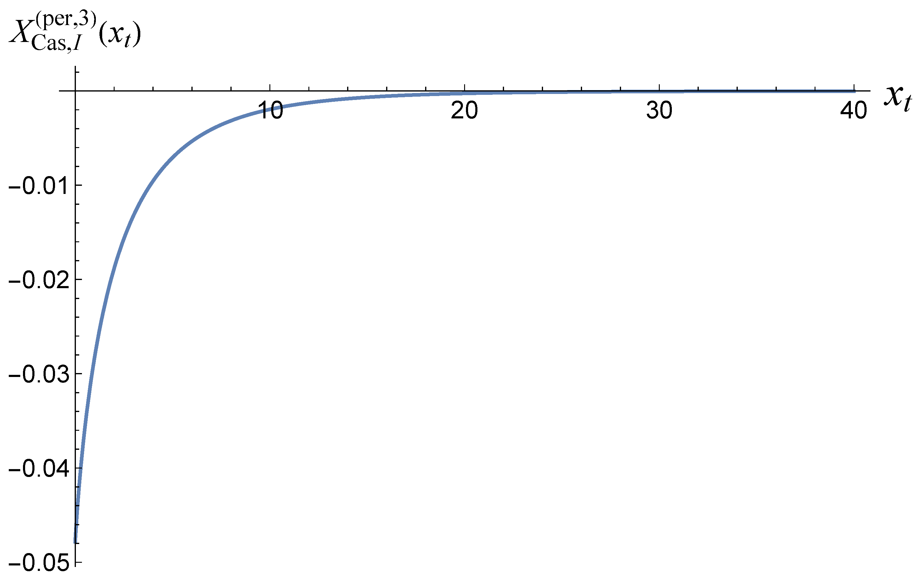
Figure 2.
The functions in (2.25)
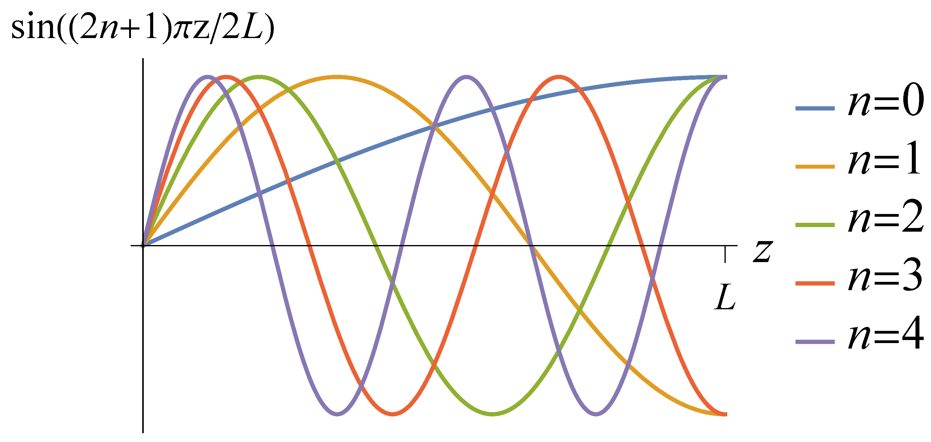
Figure 3.
The function , as given in (2.30).
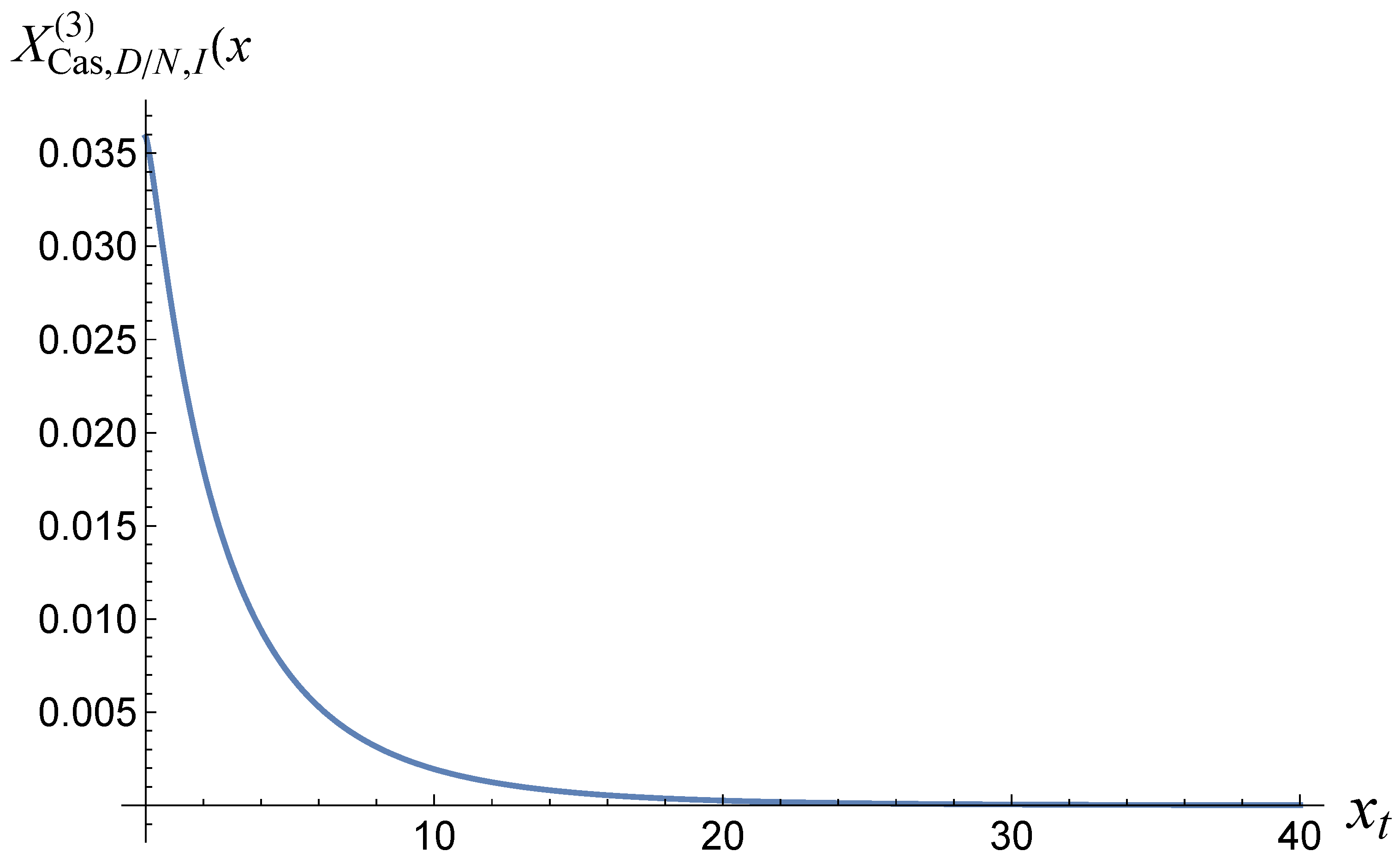
Figure 4.
The function , as given by (2.38).
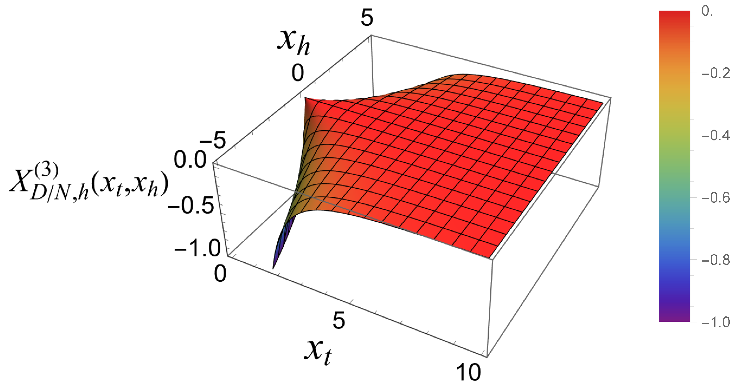
Figure 5.
The total scaling contribution to the Casimir force for Dirichlet-Neumann boundary conditions in the three dimensional Gaussian model with a scalar order parameter,. Note that this function can be both positive (repulsive) and negative (attractive).
Figure 5.
The total scaling contribution to the Casimir force for Dirichlet-Neumann boundary conditions in the three dimensional Gaussian model with a scalar order parameter,. Note that this function can be both positive (repulsive) and negative (attractive).
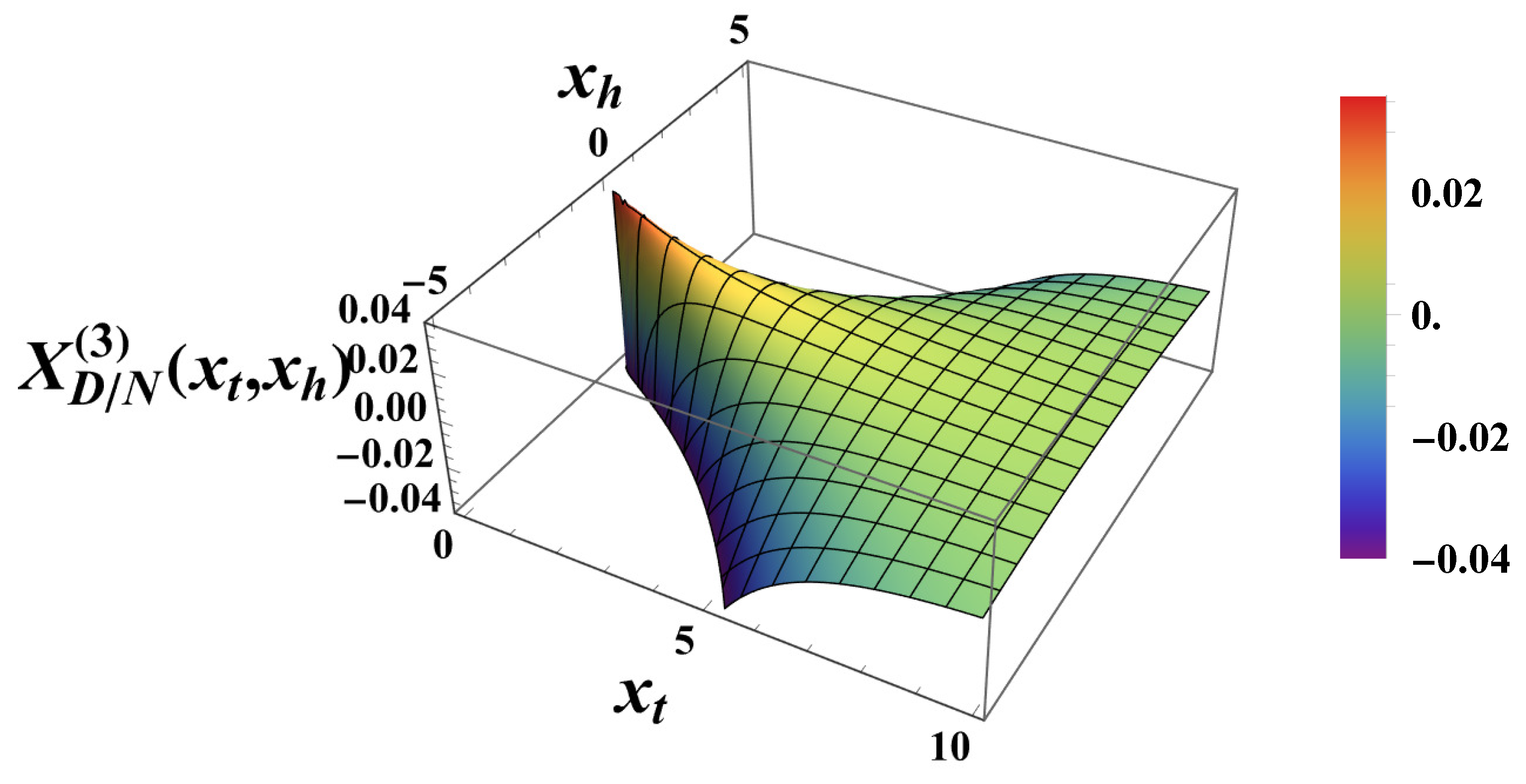
Figure 6.
The total scaling contribution to the Casimir force for Dirichlet-Neumann boundary conditions in the three dimensional Gaussian model with a scalar order parameter,. The red region in the figure corresponds to a repulsive force, and the blue region corresponds to an attractive force.
Figure 6.
The total scaling contribution to the Casimir force for Dirichlet-Neumann boundary conditions in the three dimensional Gaussian model with a scalar order parameter,. The red region in the figure corresponds to a repulsive force, and the blue region corresponds to an attractive force.
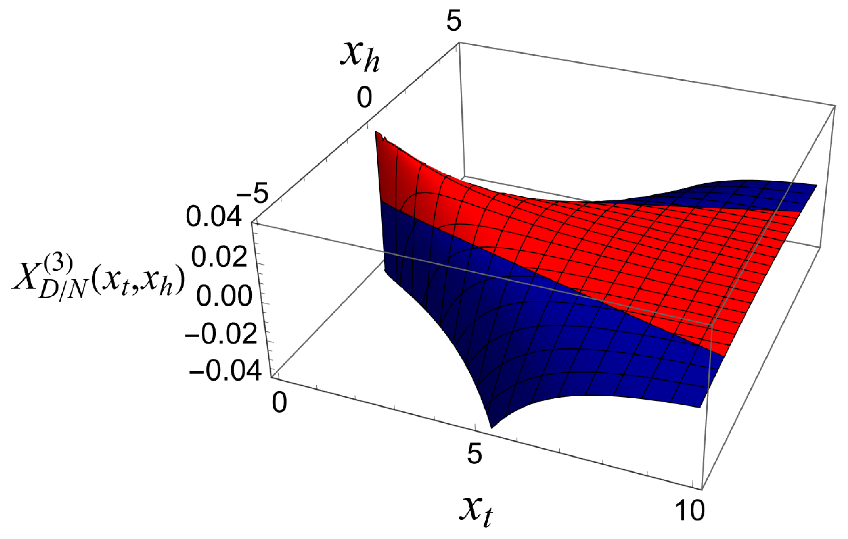
Figure 7.
The behavior of the scaling function .
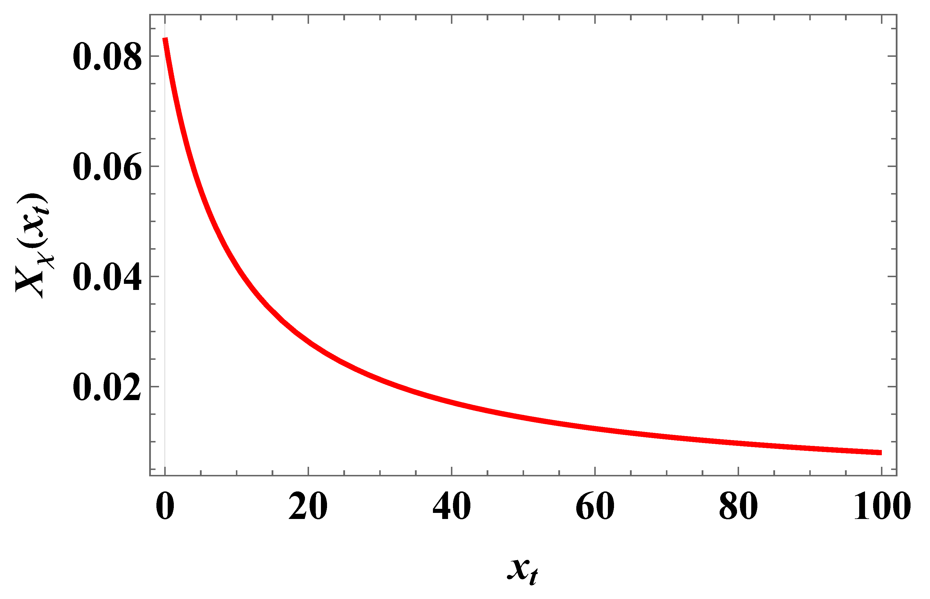
Figure 8.
The behavior of the scaling function when .
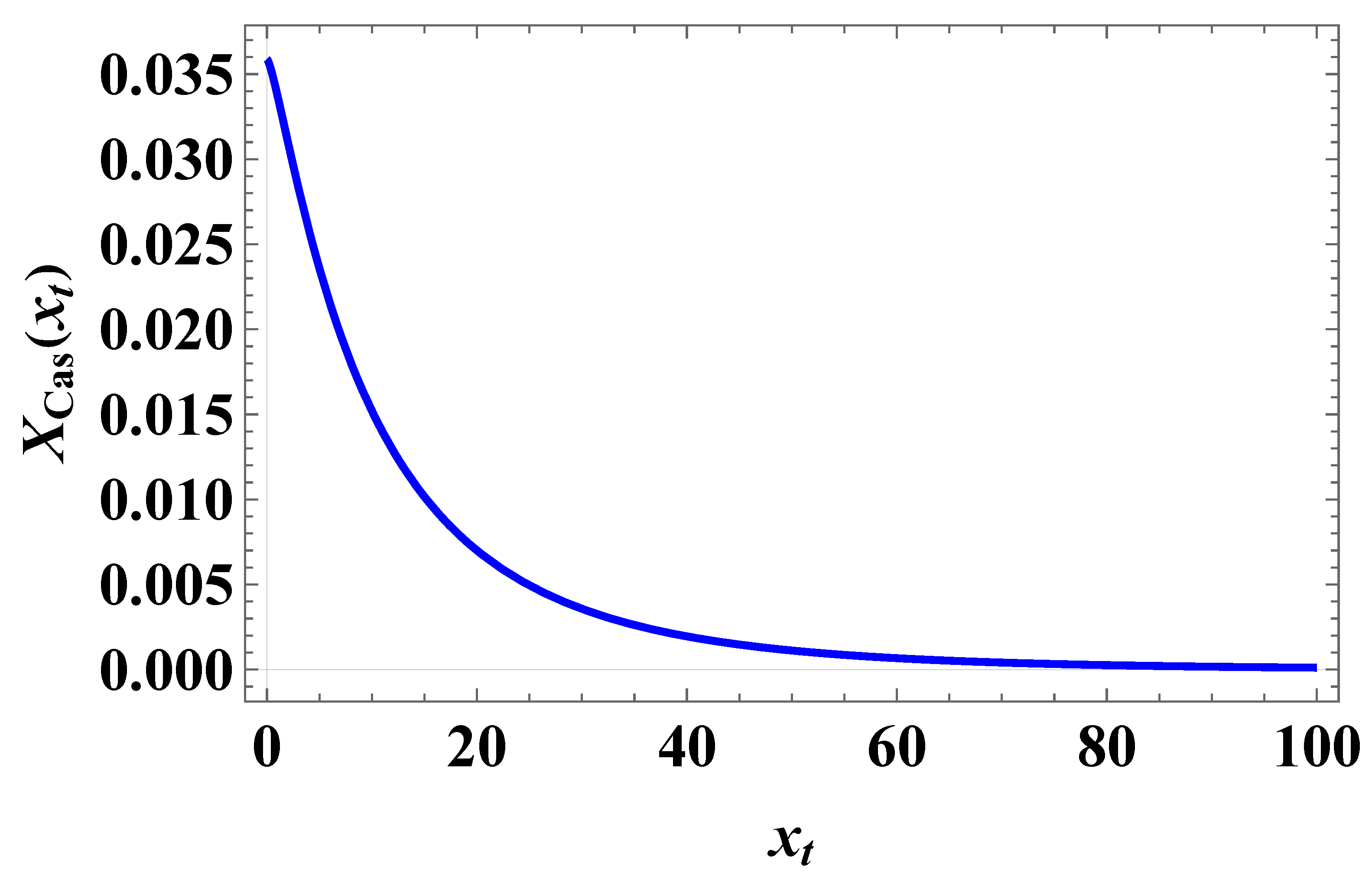
Figure 9.
The behavior of the scaling function . We observe that the force is attractive.
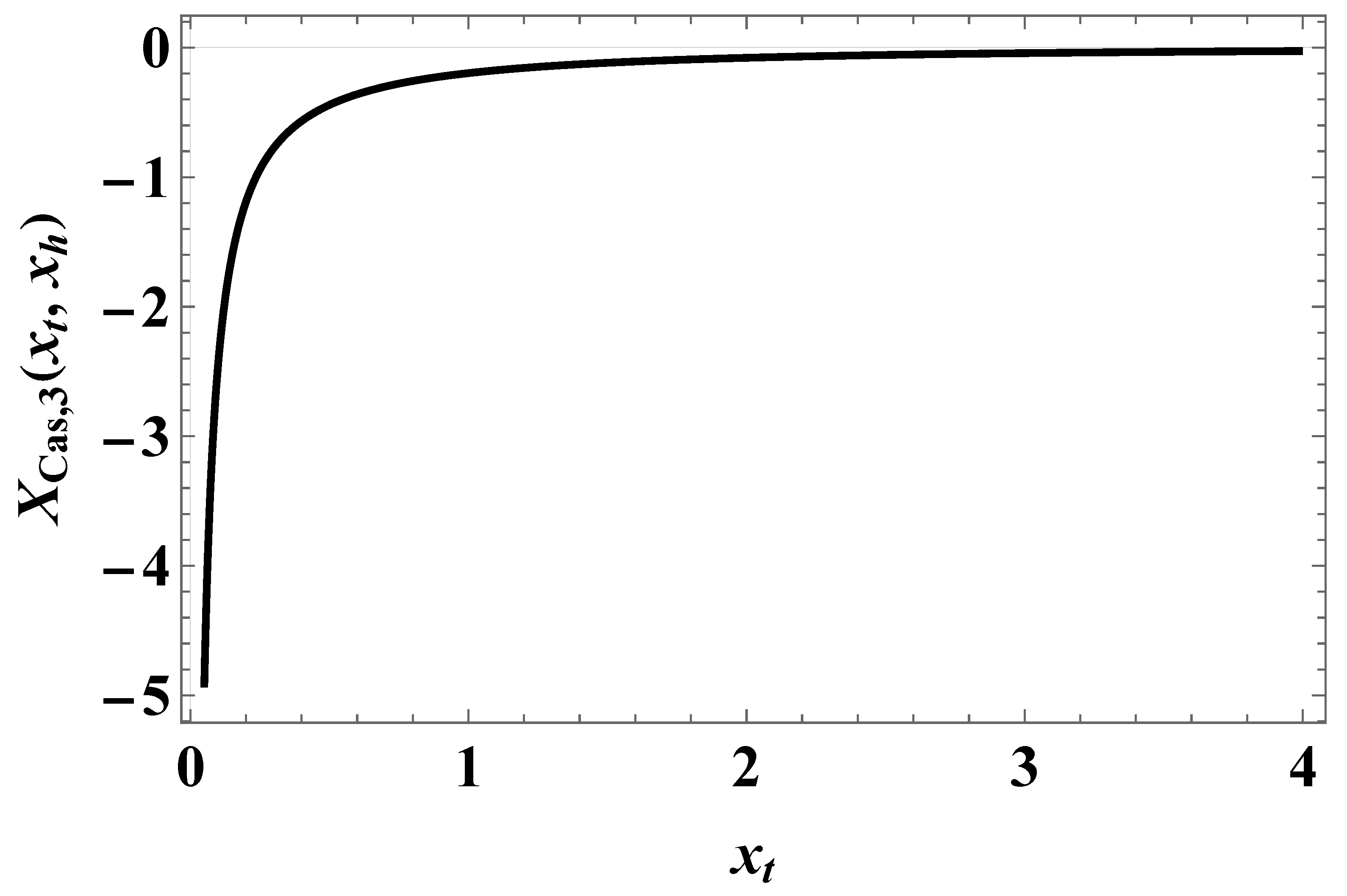
Figure 10.
The behavior of the scaling function of the total Casimir force as a function of y for several values of . Left panel: We see that for the force is attractive very near the critical temperature, then becomes repulsive with increase of (i.e., of T). Right panel: It is clear, that for zero field the force is repulsive, then — for small values of — the force changes sign from attractive to repulsive with the increase of (i.e., of the temperature), while for large values of the force becomes attractive for all values of T (i.e., ).
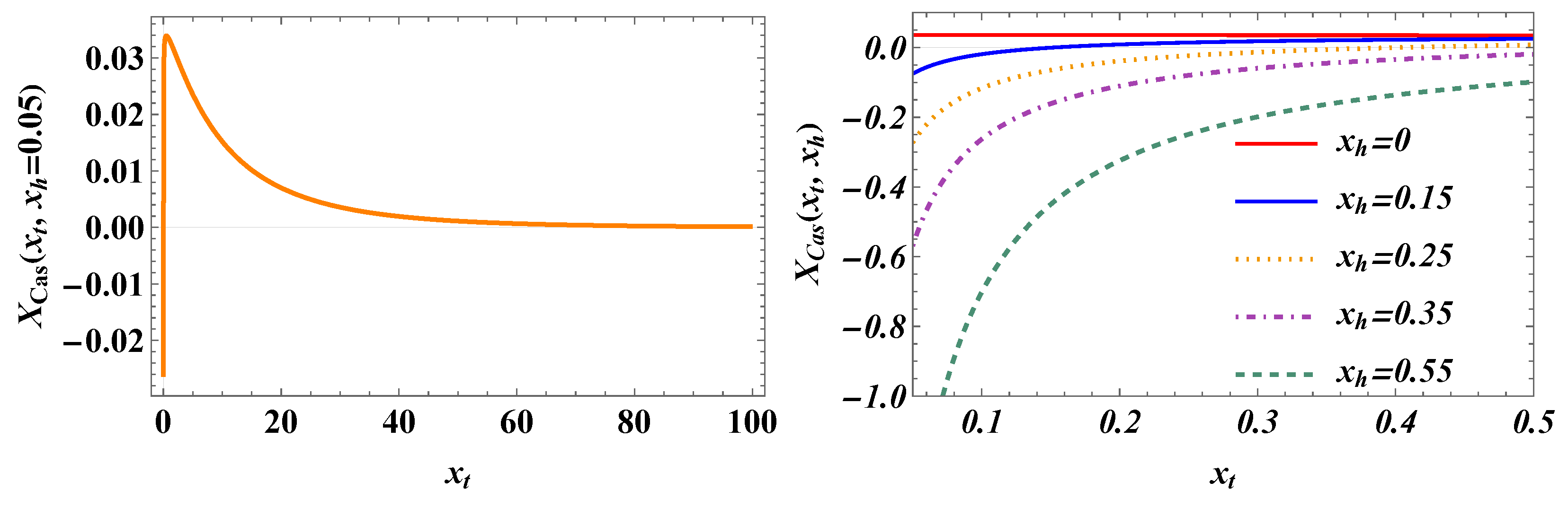
Figure 11.
The behavior of the scaling function . Here and .
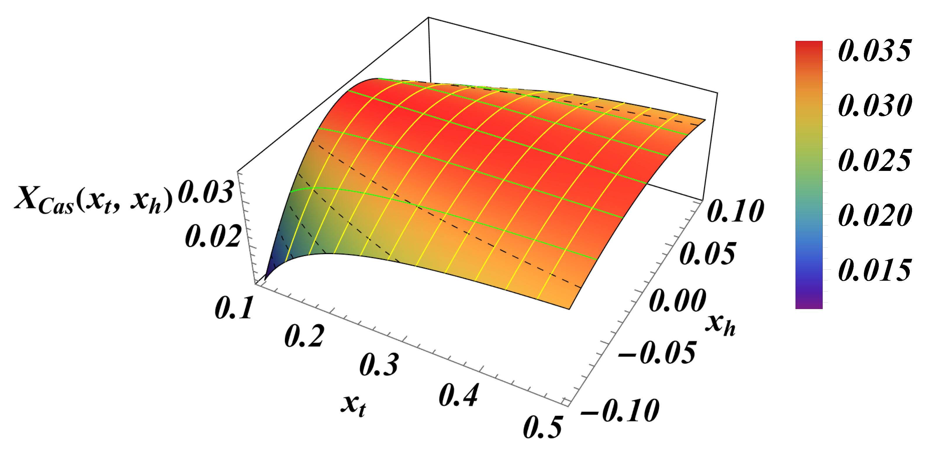
Figure 12.
Phase diagrams. Left panel: The phase diagram of the bulk system. Right panel: The phase diagram of the finite system with Dirichlet-Neumann boundary conditions. In the bulk system a phase transition of first order happens when crossing the phase coexistence line that is at and spans for . At the system exhibits a second order phase transition. In the finite system the coexistence line is at and spans for . The second order phase transition happens at . Note the change with Dirichlet-Dirichlet boundary conditions where the critical point is at .
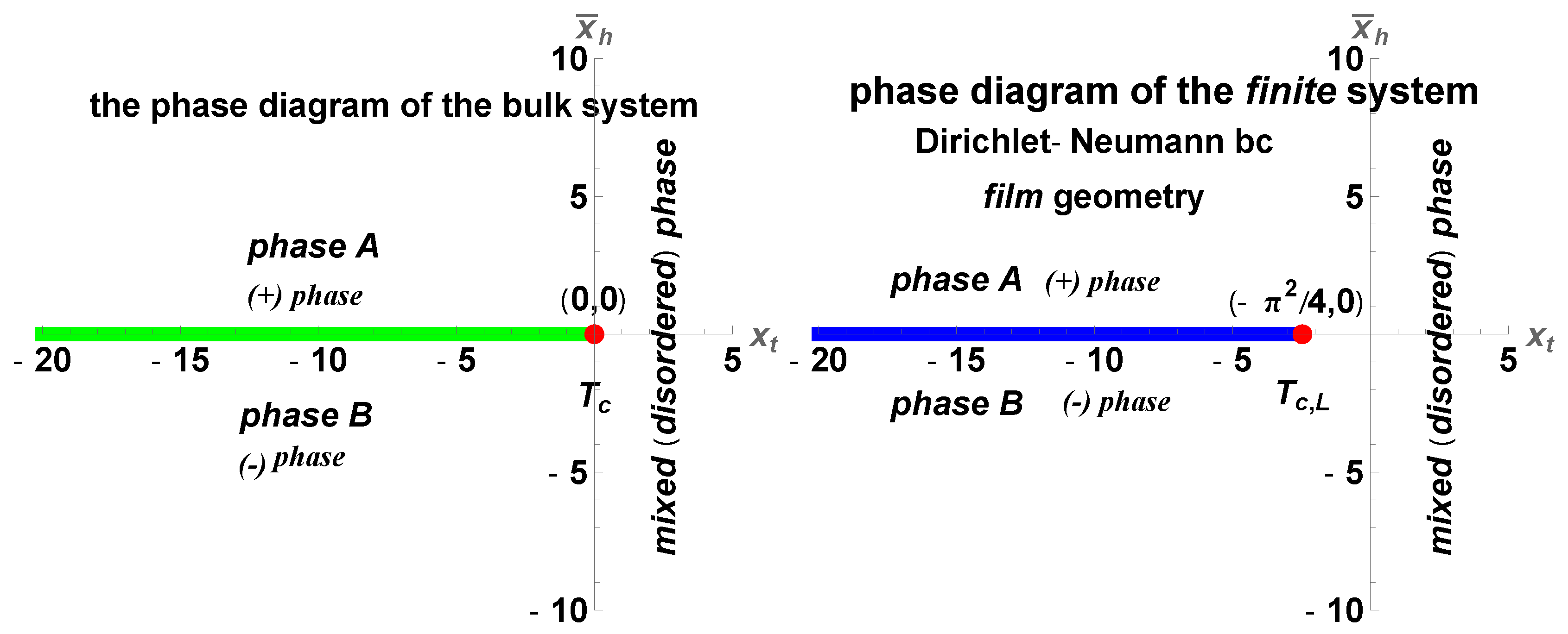
Figure 13.
The behavior of the scaling function for . We observe that the force is attractive, contrary to the corresponding result for the Gaussian model.
Figure 13.
The behavior of the scaling function for . We observe that the force is attractive, contrary to the corresponding result for the Gaussian model.
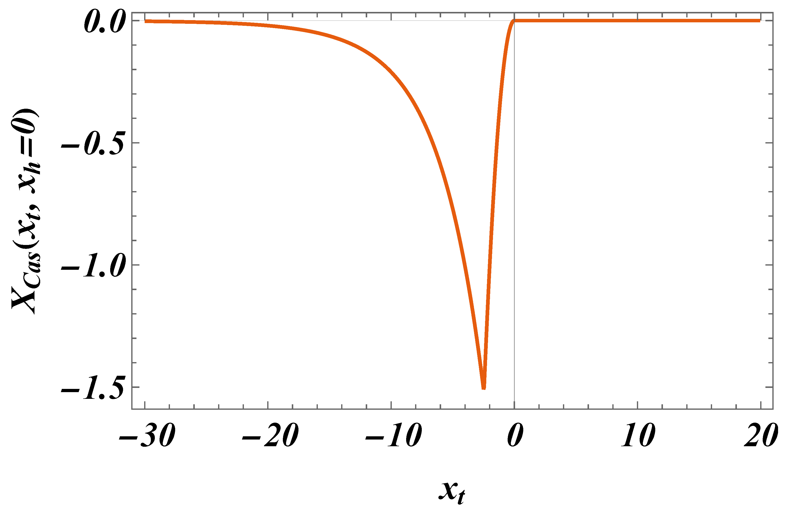
Figure 14.
The behavior of the scaling function , for several values of . We observe that the force is attractive.
Figure 14.
The behavior of the scaling function , for several values of . We observe that the force is attractive.
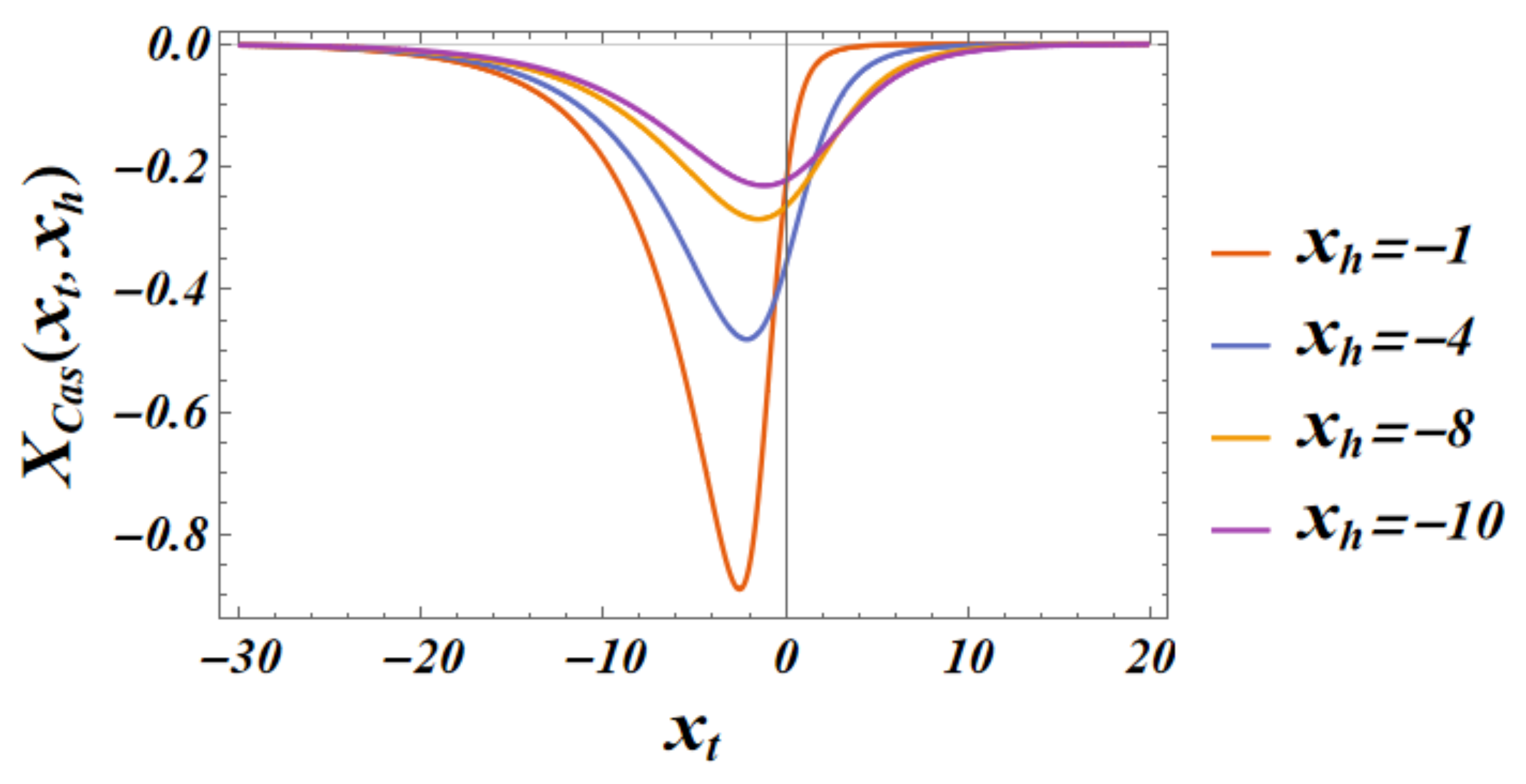
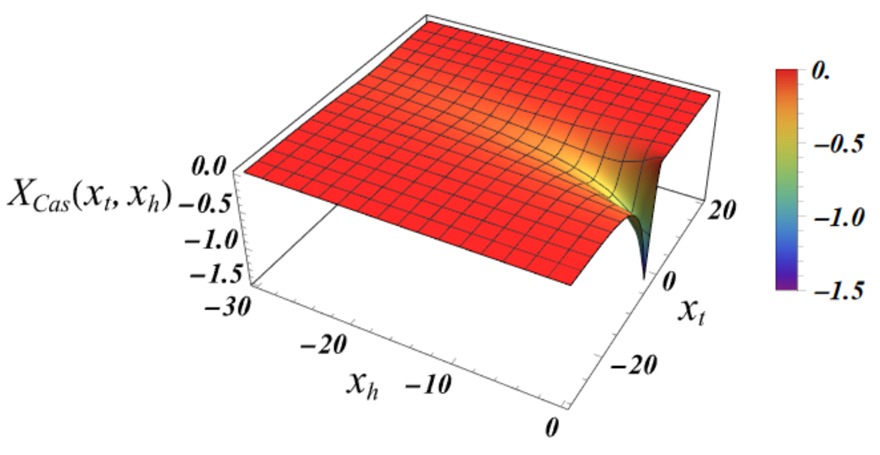
Figure 15.
The behavior of the scaling function , , . We observe that the force is attractive.
Disclaimer/Publisher’s Note: The statements, opinions and data contained in all publications are solely those of the individual author(s) and contributor(s) and not of MDPI and/or the editor(s). MDPI and/or the editor(s) disclaim responsibility for any injury to people or property resulting from any ideas, methods, instructions or products referred to in the content. |
© 2025 by the authors. Licensee MDPI, Basel, Switzerland. This article is an open access article distributed under the terms and conditions of the Creative Commons Attribution (CC BY) license (http://creativecommons.org/licenses/by/4.0/).
Copyright: This open access article is published under a Creative Commons CC BY 4.0 license, which permit the free download, distribution, and reuse, provided that the author and preprint are cited in any reuse.


