
Submitted:
03 April 2025
Posted:
03 April 2025
You are already at the latest version
Abstract
In this paper, we address the problem of obtaining bias-free and complete finite size approximations of the solution sets (Pareto fronts) of multi-objective optimization problems (MOPs). Such approximations are, in particular, required for the fair usage of distance-based performance indicators, which are frequently used in evolutionary multi-objective optimization (EMO). If the Pareto front approximations are biased or incomplete, the use of these performance indicators can lead to misleading or false information. To address this issue, we propose the Reference Set Generator (RSG), which can, in principle, be applied to Pareto fronts of any shape and dimension. We finally demonstrate the strength of the novel approach on several benchmark problems.
Keywords:
multi-objective optimization
; Pareto front approximation
; performance indicators
; benchmarking
1. Introduction
Multi-objective optimization has become an integral part of the decision-making for many real-world problems. In a multi-objective optimization problem (MOP), one is faced with the issue of concurrently optimizing k individual objectives. The set of optimal solutions is called the Pareto set. The image of the Pareto set is called the Pareto front. The latter set is, in many cases, most important for the decision maker (DM) since it provides him/her with an overview of the optimal performances for his/her project. What makes MOPs hard to deal with is that one can expect that both Pareto set and front form – at least locally and under certain assumptions on the model – objects of dimension ([1]). For the numerical treatment of MOPs, specialized evolutionary algorithms, called multi-objective evolutionary algorithms (MOEAs), have caught the interest of many researchers and practitioners during the last three decades ([2]). MOEAs are population-based and hence allow for the obtaining of a finite approximation of the entire solution set in one run of the algorithm. For the performance assessment of the outcome sets, several different indicators have been proposed so far (e.g., [3,4,5,6,7,8]). Some of these performance indicators are distance-based and require a “suitable” finite-size representation of the Pareto front. While until now, a vast variety of different MOEAs has been proposed and analyzed, it is fair to say that the generation of suitable reference sets has played a rather minor role in the evolutionary multi-objective optimization (EMO) community. It is evident that such reference sets should be complete. Further, as we show in this work, a biased representation can lead to misleading or even false information.
To fill this gap, we propose in this work the Reference Set Generator (RSG). The main steps of RSG are as follows: (i) a first approximation of the Pareto front is either taken or generated. This set can be, in principle, of arbitrary size, and the elements can be non-uniformly distributed along the Pareto front (i.e., biased). However, all of these elements have to be "close enough" to the set of interest. In order to obtain a bias-free approximation, (ii) component detection and (iii) a filling step is applied to . Finally, (iv) a reduction step is applied. The RSG is applicable to MOPs with Pareto fronts of, in principle, any shape and dimension. Further, the resulting reference set is of any desired magnitude. We will show the strength of the novel method on several benchmark problems.
The remainder of this paper is organized as follows: in Section 2, we briefly recall the background for the understanding of this work. We further discuss the related work and the performance indicators that benefit from our approach. In Section 3, we first motivate the need for bias-free complete finite-size Pareto front approximations, and propose the Reference Set Generator (RSG). In Section 4, we present some numerical results on selected benchmark problems and compare the RSG to related algorithms. Finally, we draw our conclusions in Section 5 and give possible paths for future research.
2. Background and Related Work
We consider multi-objective optimization problems (MOPs) that can be mathematically expressed via
Hereby, the map F is defined as
where we assume each of the individual objectives , , to be continuous. We stress, however, that the method we propose in the sequel, RSG, can, in principle, also be applied to discrete problems. Q is the domain of the objective functions that is typically expressed by equality and inequality constraints.
In order to define the optimality of an MOP, one can use the concept of dominance [9].
Definition 1.
(a) Let . Then the vector v is less than w (), if for all . The relation is defined analogously.
- (b)
- is dominated by a point () with respect to (MOP) if and .
- (c)
- is called a Pareto point or Pareto optimal if there is no that dominates x.
- (d)
- The set of Pareto optimal solutionsis called the Pareto set.
- (e)
- The image of the Pareto set is called the Pareto front.
One can expect that both the Pareto set and the Pareto front form under certain conditions, at least locally objects of dimension . For details, we refer to [1]. Due to this "curse of dimensionality" It is, hence, not possible for an evolutionary multi-objective optimization algorithm (MOEA) to keep all promising candidate solutions (e.g., all non-dominated ones) during the algorithm run. It is, hence inevitable – at least for continuous problems – to select which of the promising solutions should be kept in order to obtain a "suitable" approximation of the solution set (in most cases, the Pareto front of the given MOP). Within MOEAs, this process is termed "selection". Another term, which can be used synonymously, is "archiving". The latter is typically used when the MOEA is equipped with an external archive.
Most of the existing MOEAs can be divided into three main classes: (a) MOEAs that are based on the concept of dominance (e.g., [10,11,12,13]), (b) MOEAs that are based on decompositions (e.g., [14,15,16,17,18]), and (c) MOEAs that make use of an indicator function (e.g., [19,20,21,22,23]). The selection strategies of the first generation of MOEAs of class (a) are based on a combination of non-dominated sorting and niching (e.g., [24,25,26]). Later, elite preservation was included, leading to an increased overall performance (and, as a consequence, better Pareto front approximations). This holds, e.g., for SPEA ([27]), PAES ([13]), SPEA-II ([11]), and NSGA-II ([10]). Theoretical studies on selection mechanisms have been done by the groups of Rudolph ([28,29,30,31]) and Hanne ([32,33,34,35]). All of these selection mechanisms deal with the abilities of the populations to reach the Pareto set/front. On the other hand, the distributions of the individuals along the Pareto sets/fronts have not been considered. The selection mechanisms of the MOEAs within classes (b) and (c) follow directly from the construction of the algorithms: selection in a MOEA of class (b) is done by considering the values of the chosen scalarization functions. Analogously, the selection in a MOEA of class (c) is done by considering the indicator contributions.
Existing (external) archiving strategies can also be divided into three classes: (a) unbounded archivers, (b) implicitly bounded archivers, and (c) bounded archivers. Unbounded archivers store all promising solutions during the algorithm run. The magnitudes of such archives can exceed any given threshold if the algorithm is run long enough. Unbounded archivers have, e.g., been used and analyzed in [36,37,38,39,40,41,42]. -dominance ([43]) can be viewed as a weaker concept of dominance. This relation allows single solutions to “cove” entire parts of the Pareto front of a given MOP, which is the basis for most implicitly bounded archivers. Such strategies have first been considered in the context of evolutionary multi-objective optimization (EMO) by Laumanns et al. ([44]). Later works proposed and analyzed different approximations (such as gap-free approximations of the Pareto front) and deal with different sets of interest (e.g., the consideration of all nearly optimal or all -locally optimal solutions), ([40,41,45,46,47,48,49,50]). Finally, bounded archivers have, e.g., been proposed in [51,52] where adaptive grid selections have been utilized. Bounded archivers tailored to the use of the Hypervolume indicator have been suggested in [53,54]). Laumanns and Zenklusen have proposed two bounded archivers that aim for -approximations of the Pareto front ([55]).
All of the selection/archiving strategies mentioned above have in common that they aim for a "best approximation" of the set of interest out of the given (finite) data. A related but slightly different problem is to generate a "suitable" (in particular complete and bias-free) finite size approximation of the set of interest S for the sake of comparisons, even if S is known approximately or even analytically but not “trivia” (e.g., a line segment). Tian et al. [56] describe the procedure of PlatEMO [57], which uses uniform sampling on the simplex and then maps these points to the particular Pareto front of each problem. However, an analytical expression or characterization of the Pareto front is required, and in some cases, the obtained set is not completely uniform. A method related to RSG can be found in [58] which has the aim of guiding the iterates of a particular Newton method toward the Pareto front. In this work, we extend this idea for the purpose of generating complete and bias-free Pareto front approximations of relatively large magnitudes (in particular compared to population sizes used in EMO).
Finally, reference sets as the ones generated by RSG are helpful for the evaluation of the performance qualities of candidate sets (populations) in EMO. More precisely, such sets are required for all distance-based indicators. The earliest such indicators are the Generational Distance (GD, [3]) and the Inverted Generational Distance. (IGD, [5]). Later, the indicator ([6,59]) has been proposed that is a combination of slight variants of GD and IGD, and that can be viewed as an averaged version of the Hausdorff distance . So far, there exist several extensions of these performance indicators. For instance, the consideration of continuous sets – either only the Pareto front or also the candidate solution set – has been done in [8,60] leading to modifications of and . The indicators IGD+ ([7]) and DOA ([61]) are modifications of IGD that are Pareto compliant.
3. Reference Set Generator (RSG)
In this section, we first motivate the need for complete and bias-free finite size Pareto front approximations, and then propose the Reference Set Generator (RSG) that targets for such sets.
3.1. Motivation
Distance-based indicators require a “suitable” finite-size approximation of the Pareto front in order to give a "correct" value for the approximation quality of the considered candidate solution set. This holds in particular for the above-mentioned indicators GD, IGD, and , together with their variants. Such representations are ideally uniformly spread along the entire Pareto front ([60]). This, however, is a non-trivial task unless the Pareto front is given analytically and has a relatively simple form (e.g., linear or perfectly spherical). Regrettably, this is the case for only a few test problems (e.g., DTLZ1 and DTLZ2). On the other hand, there exist quite a few benchmark MOPs where the shape of the Pareto set is relatively simple. For such problems, it is tempting to choose uniform samples from the Pareto set (i.e., , where all ), and to use the respective image to represent of the Pareto front. The following discussion shows, however, that this approach has to be handled with care since it can induce unwanted biases in the approximations that, in turn, may result in misleading indicator values.
As the first example, consider the one-dimensional bi-objective problem
Let the domain be given by , then the Pareto set is identical to Q, and the Pareto front is the line segment that connects the points and . Figure 1 shows the result when using N equally spaced points along the Pareto set. As it can be seen for and , there is a clear bias of the images toward the right lower end of the Pareto front. For , the Pareto front approximation is "complete" (at least from the practical point of view) and appears to be perfect. However, it possesses the same bias. To see the impact of the reference set on the performance indicators consider the two hypothetical outcomes (e.g., possible results from different MOP solvers):
Figure 2 shows the two sets together with the Pareto front. Note that A is the perfect 5-element approximation of the Pareto front: the elements are equally distributed along the Pareto front, and the extreme points are shifted “half-way in” ([60]). The set B is certainly not perfect as it, e.g., misses to "cover" more than half of the front. Table 1 shows values for different distance-based indicators, the outcomes , and different representations R of the Pareto front. For (the one shown in Fig. 1 (c)), all indicators – except – yield lower values for B than for A, indicating (erroneously) that B is better than A. This is not the case for since the Hausdorff distance is determined by the maximum of the considered distances and not by an average of those (however, has other disadvantages in the context of EMO, most prominently that it punishes single outliers [6]). The situation changes when selecting as a representation of the front. This representation also contains elements, but these are chosen uniformly along the Pareto front. Now, there is a tie for the two GD variants, and for all other indicators, A leads to better values than B. These values are indeed very close to the `correct’ values: all exact GD values are equal to zero since A and B are contained in the Pareto front. In order to compute the exact IGD values, a particular integral has to be solved [60]. When using as representation, the computation of the IGD values can be interpreted as a Riemann sum with equally sized sub-intervals leading to perfect solutions, at least from the practical point of view.
We repeat the process, but now using only elements for the representation (see Table 1). We can see the same trend, i.e., that B appears to be better for while A appears to be better when using . Further, we see that the indicator values for are already quite close to the exact values (i.e., when using ). While the proper choice of N may not be an issue for bi-objective problems (), this may get important for a larger number of objectives due to the “curse of dimensionality”: at least for continuous problems, one can expect that the Pareto front forms under certain (mild) assumptions a manifold of dimension ([1]).
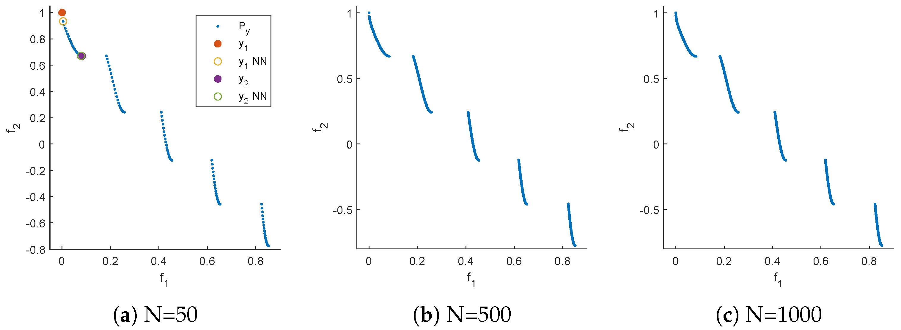
We next consider further test problems. Figure 4, Figure 5 and Figure 6 show the Pareto front approximations for the commonly used test problems DTLZ1, ZDT1, and ZDT3, respectively, where the representation has been obtained via uniform sampling in decision variable space along the Pareto set. In all cases, the Pareto front representations appear to be perfect for large enough values of N. However, certain biases can be observed for lower values of N. For all test problems, we selected two points out of the representation and showed their nearest neighbors. These values differ by one order of magnitude which confirms that the solutions are not uniformly distributed along the fronts. Using such representations, the same issues can arise as discussed above.
To conclude, the suitable representation of the Pareto front of a given MOP is crucial when considering distance-based performance indicators that use an average of the distances considered. Such representations are ideally equally distributed over the front. If the representation contains a bias, this may result in misleading indicator values, leading, in turn, to a wrong evaluation of the obtained results. In particular, the approach to performing the sampling along the Pareto set is, though tempting, not appropriate for such indicator-based indicators. In the sequel, we will propose a method that aims to achieve a uniform Pareto front representations.
Figure 3.
Distribution resulting from uniformly sampling the Pareto set of DTLZ1 with N points. In (a) , .
Figure 3.
Distribution resulting from uniformly sampling the Pareto set of DTLZ1 with N points. In (a) , .
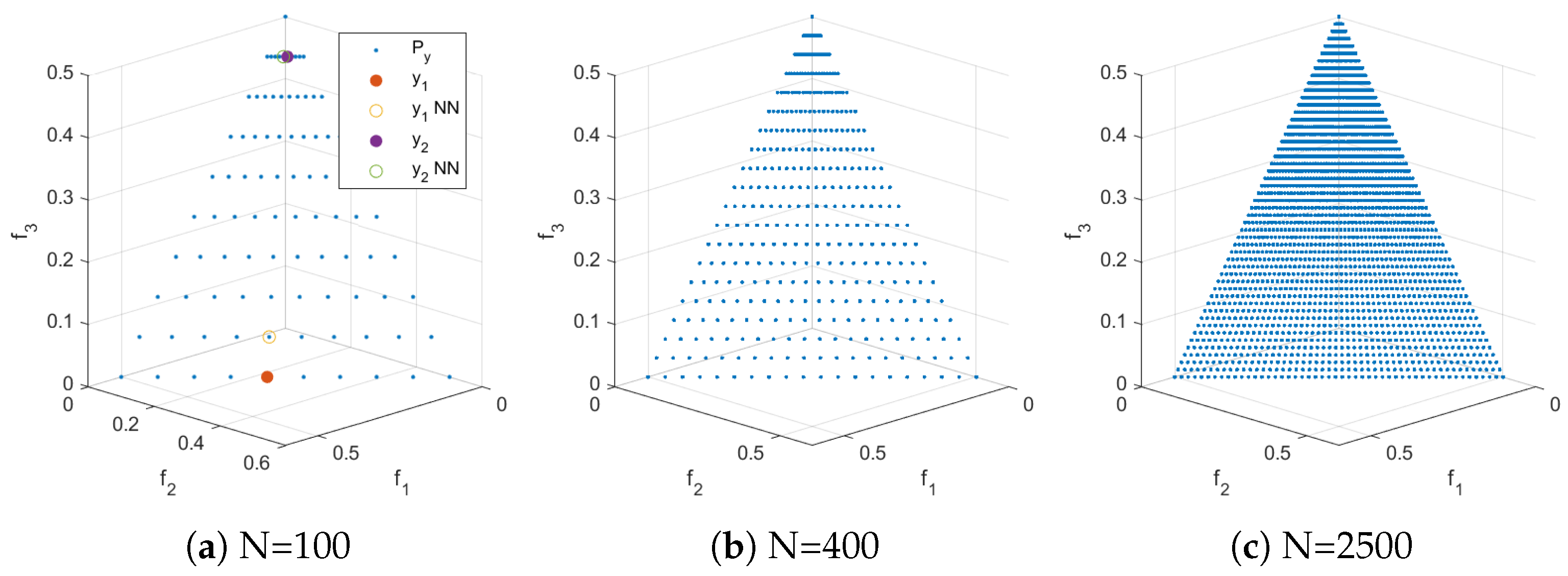
Figure 4.
Distribution resulting from uniformly sampling the Pareto set of DTLZ2 with N points. In (a) , .
Figure 4.
Distribution resulting from uniformly sampling the Pareto set of DTLZ2 with N points. In (a) , .
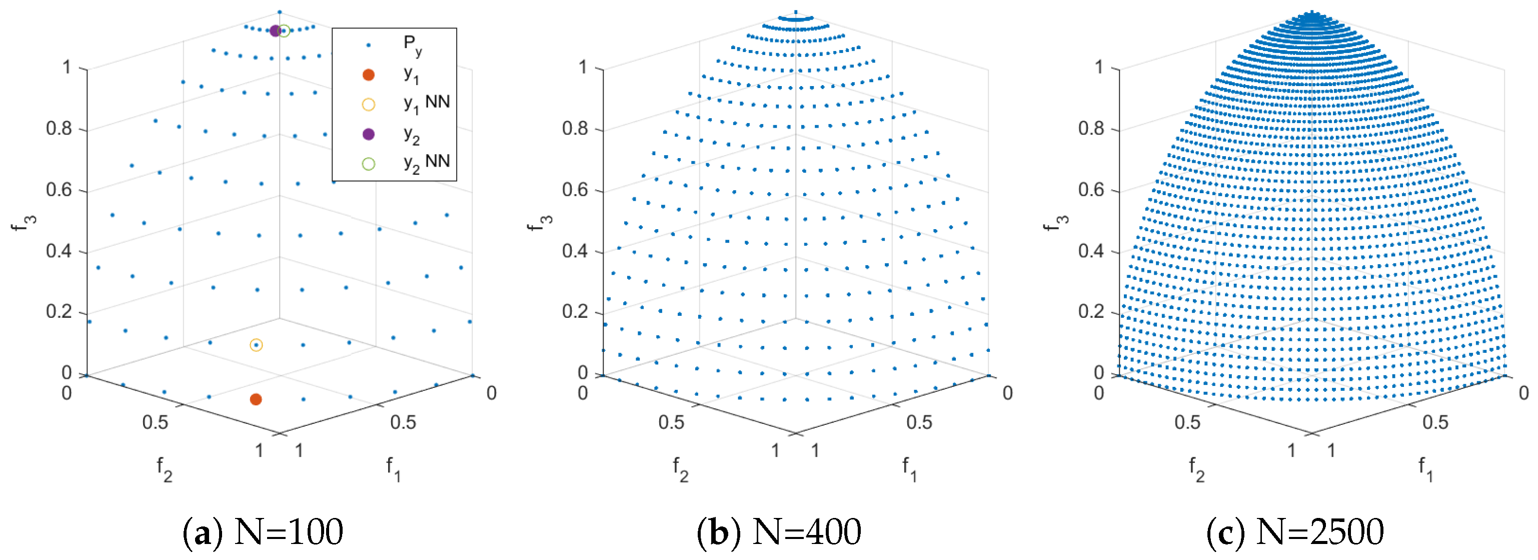
Figure 5.
Distribution resulting from uniformly sampling the Pareto set of ZDT1 with N points. In (a) , .
Figure 5.
Distribution resulting from uniformly sampling the Pareto set of ZDT1 with N points. In (a) , .
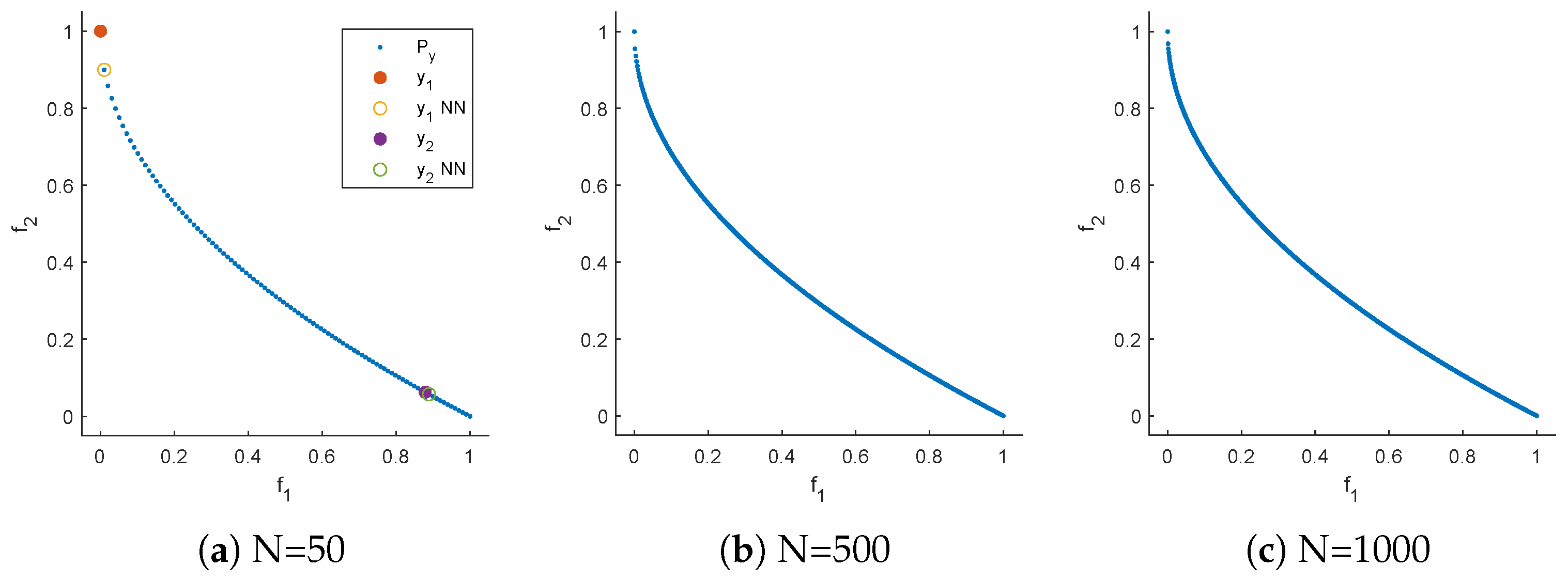
Figure 6.
Distribution resulting from uniformly sampling the Pareto set of ZDT3 with N points. In (a) , .
Figure 6.
Distribution resulting from uniformly sampling the Pareto set of ZDT3 with N points. In (a) , .
3.2. RSG
In the following, we assume we are interested in a Pareto front approximation of size N for a given MOP. Further, we assume that we are given a set of (in principle) arbitrary size ℓ of non-dominated, possibly non-uniformly distributed points that are "close enough" to the PF. Below, we will discuss different strategies to obtain . Given this data, the Reference Set Generation (RSG) process consists of three main steps: component detection, filling, and reduction. The idea is to fill the gaps between the points within each connected point of . This leads to a more complete set F with a higher cardinality than , which can then be reduced to obtain a uniform reference set of size N. In general, PFs can be disconnected, and if we simply fill the gaps in , we may introduce points that do not belong to the PF (Figure 7(b)). Therefore, component detection must be performed before applying the filling process to each detected component (Figure 7(a)).
The general procedure of RSG is presented in Algorithm 1, and each of the main steps will be explained in the following subsections. Figures 8, 12, 9, and 13 illustrate all the steps for the problems ZDT3, CONV3-4, DTLZ7 and CONV4-2F. It is important to note that the cases for and objectives exhibit slight variations in the component detection step and follow completely different procedures for the filling step.
| Algorithm 1 Reference Set Generation (RSG) |
|
3.3. Component Detection
Since the PF might be disconnected, we first apply a component detection on . We use DBSCAN [62] in the objective space for this purpose for three main reasons: (i) the number of components does not need to be known a priori, (ii) the method detects outliers, and (iii) we have observed that a density-based approach works better than a distance-based one (e.g., k-means) for component detection. DBSCAN has two parameters: and r. To make the component detection process “parameter-free”, we compute a small grid-search to find the optimal values of and r based on the weakest link function defined in [63]. The default parameter values are and for bi-objective problems, and and otherwise, where is the average pairwise distance between all points. However, these parameters can be adjusted when calling RSG. A summary of the component detection process is presented in Algorithm 2. In the following, we describe the remaining steps for a single connected component. If multiple components exist, the procedures must be repeated analogously for each component identified by Algorithm 2.
| Algorithm 2 Component Detection |
|
3.4. Filling
Even if we know the PS a priori, a uniform sampling of the PS will not result in a uniform sampling of the PF. We assume that we have a set of points that is not uniformly distributed. However, if we fill the gaps and select N points from the filled set, we can obtain a more uniform set, leading to better IGD approximations when selecting points from these filled sets. The idea behind the filling step is to create a set that is as uniform as possible, so that the reduction step (in particular, k-means) does not get stuck in non-uniform local optima, which would lead to non-uniform final sets. The next task is, therefore, to compute solutions that are ideally uniformly distributed along .
This process is performed differently for and objectives:
- For , we sort the points of in increasing order of , i.e., the first objective. Then, we consider the piecewise linear curve formed by the segments between and , and , and so on. The total length of this curve is given by , where . To perform the filling, we arrange the desired points along the curve L such that the first point is and the subsequent points are distributed equidistantly along L. This is achieved by placing each point at a distance of from the previous one along L. See Algorithm 3 for details.
-
The filling process for consists of several intermediate steps that must be described first; see Algorithm 4 for a general outline of the procedure. The procedure is as follows: First, to better represent (particularly for the filling step), we triangulate this set in dimensional space. This is done because the PF for continuous MOPs forms a set whose dimension is at most . To achieve this, we compute a “normal vector” to using equation 9, and then we project it onto the hyperplane normal to , obtaining the projected set . After this, we compute the Delaunay triangulation [64] of , which provides a triangulation that can be used in the original k-dimensional space. For concave PFs, the triangulation may include triangles (or simplex for ) that extend beyond (Figure 12(d)), so a removal strategy is applied to eliminate these triangles and obtain the final triangulation T. Finally, each triangle is uniformly filled at random with a number of points proportional to its area (or volume for ), resulting in the filled set F of size .We will now describe each step in more detail in the following:
- −
- Computing “normal vector” . Since the front is not known, we compute the normal direction orthogonal to the convex hull defined by the minimal elements of . More precisely, we compute as follows: if , choosewhere denotes the i-th element of , and setNext, compute a QR-factorization of M, i.e.,where is an orthogonal matrix with column vectors , and is a right upper triangular matrix. Then, the vectoris the desired shifting direction. Since Q is orthogonal, the vectors form an orthonormal basis of the hyperplane that is orthogonal to . That is, these vectors can be used for the construction of .
- −
- Projection . We use as the first axis of a new coordinate system , where the vectors are defined as above. In this coordinate system, the orthonormal vectors form the basis of a hyperplane orthogonal to . The projection of onto this hyperplane () is achieved by first expressing in this new coordinate system as , and then removing the first coordinate, yielding .
- −
- Delaunay Triangulation . Compute the Delaunay triangulation of . This returns , a list of size containing the indices of that form the triangles (or simplices for ). The list serves as the triangulation for the k-dimensional set , which is possible because consists of indices, making it independent of the dimension. We use to denote the number of triangles obtained, the indices of the vertices forming triangle i and to denote the corresponding vertices of triangle i.
- −
- Triangle Cleaning . We identify three types of unwanted triangles: those with large sides, those with large areas, and those where the matrix containing the coordinates of the vertices has a large condition number. The type of cleaning applied depends on the problem; however, the procedure remains the same for any problematic triangle case and is outlined in Algorithm 5. First, the property (area, largest side, or condition number) is computed for all the triangles . Next, triangles i with are removed. The parameter is also problem-dependent, and the specific values used for each problem will be detailed in the results section.
- −
- Triangle Filling . For each triangle with area , we generate points uniformly at random inside triangle , following the procedure described in [65]. That is, the number of points is proportional to the area (or volume) of each triangle (or simplex). Here, is the total area of the triangulation.
| Algorithm 3 Filling ( Objectives) |
|
| Algorithm 4 Filling ( Objectives) |
|
| Algorithm 5: Triangle Cleaning |
|
3.5. Reduction
Once we have computed the filled set F, we need to select N points that are ideally evenly distributed along F. To this end, we use k-means clustering with N clusters, as there is a strong relationship between k-means and the optimal subset selection ([66,67]). The resulting N cluster centroids form the PF reference set Z. Note that this reduction method can be modified if needed to obtain an ideal reference according to other types of indicators (i.e., those that are not distance-based).
3.6. Obtaining
RSG requires an initial approximation of the Pareto front. Note that by construction of the algorithm, this set can have small imperfections (which can be removed by the filling step) and can also have biases in the approximation (reduction step). However, it is desired that "captures" the shape of the entire Pareto front. The computation of such an approximation is certainly problem-dependent. For our computations, we have used the following three main procedures to get :
- sampling: For some benchmark problems, either the Pareto set or the Pareto front is given in analytic form. If a sampling can be performed in objective space (e.g., for linear fronts, the remaining steps of the RSG may not be needed to further improve the quality of the solution set. If the sampling is performed in decision variable space, the elements of the resulting image may not be uniformly distributed along the Pareto front as discussed above. However, in that case, the filling and reduction step will help to remove biases.
- archiving: The result of an MOEA or any other MOP solver can, of course, be taken. This could be either the final archive of the population, via merging several populations of the same or several runs ([58]), or via using external (unbounded) archives ([50]). Note that this includes taking a reference set from a given repository. We have used archiving, e.g., for the test problems WFG3-9, DTLZ1-4, DTLZ7, ZDT1-6, CONV3, CONV3-4, and CONV4-2F.
- continuation: An alternative to the above mentioned techniques is to make use of multi-objective continuation methods, probably in combination with the use of several different starting points. In particular, we have used the Pareto Tracer (PT, [68,69,70]), a state-of-the-art continuation method that is able to treat problems of in principle any dimensions (both n and k), can handle general constraints and that can even detect local degeneration of the solution set. We have used PT, e.g., for the test problem WFG1, WFG2, DTLZ5, and DTLZ6.
3.7. Complexity Analysis
The overall complexity is for (regardless of the number of components), and for , where ℓ is the size of the initial approximation , k is the number of objectives, is the number of triangles in the Delaunay triangulation, is the number of iterations of k-means (bounded to 500 in this work), N is the desired size of the reference set Z, and is the size of the filling. This assumes and that the triangle-cleaning method used is based on the longest side (which was the method applied to all the references presented in this work). Typically, obtaining a decent approximation requires a large value of , making the clustering step the dominant one and thus reducing the overall complexity to for any k. We now present the complexity analysis in detail for each step separately, considering a single component. We now present the complexity analysis in detail for each step separately, considering a single component.
- Component Detection. The time complexity is which accounts for the computation of the average distance, plus the size of the grid search () multiplied by the sum of the complexities of DBSCAN and the WeakestLink computation. Here, ℓ is the size of , and represents the number of parameter combinations of the grid search, with for and for using the default values. If it is previously known that the Pareto front is connected, then the parameters of DBSCAN can be correctly adjusted, and can be set to 1.
-
Filling. The time complexity depends on the number of objectives:
- −
- For the time complexity is , which accounts for sorting and placing the points along the line segments.
- −
- For the time complexity is due to the computations involved in determining the normal vector , changing coordinates and projecting, performing the Delaunay triangulation, and filling the triangles. Here, represents the size of the cleaned Delaunay triangulation, i.e., the number of triangles. Additionally, triangle cleaning must be considered, though its complexity depends on the method used. It is given by when cleaning is based on area or the condition number (due to determinant computation), or when cleaning based on the longest side.
- Select Reference Set T. The time complexity is due to the k-means clustering algorithm. Here, is the number of iterations of k-means.
4. Results
In this section, we show the strength of the novel approach to selected test problems. We further show – as far as possible – comparisons to related methods.
First, we show all the steps of the RSG on five representative problems: Figure 8 shows these steps for ZDT3 ( and disconnected), Figure 9 for DTLZ7 ( and disconnected), Figure 11 for CONV3 (defined in Appendix A, ), Figure 12 for CONV3-4 (defined in Appendix A, ) and Figure 13 for CONV4-2F (defined in Appendix A, and disconnected).
In Figure 8 and Figure 9, we have used starting sets that have a slight bias. The last subfigures show the results of RSG for different values of N. For Figure 11, Figure 12 and Figure 13, we demonstrate the universality of RSG, as it does not need any analytical information of the PF since it utilizes the result of a MOEA and an archiver to generate a reference of any desired size.
Additionally, a comparison between RSG, PlatEMO [57], Pymoo, and the filling step is presented in Figure 14 and Figure 15 for the WFG2, ZDT1, ZDT3, DTLZ2, Convex DTLZ2 (CDTLZ2), C2-DTLZ2, and DTLZ7 test problems. Although the reference sets provided by PlatEMO and Pymoo are of high quality, they still exhibit some bias in certain bi-objective problems (such as ZDT1 and ZDT3), and especially in three-objective problems such as WFG2, and CDTLZ2. Furthermore, for problems like WFG2, and DTLZ7, the number of points in the reference sets of PlatEMO and Pymoo is limited to a fixed set, in contrast to RSG, which can generate any desired number of points.
Upon acceptance of this paper, we will provide reference sets on our website http://neo.cinvestav.mx:3005/ for the problems considered in this work as well as other problems (in the future, we intend to provide data for all commonly used benchmark test functions). The website will allow users to request reference sets of any desired size for any of the aforementioned problems. Further, the codes of RSG will be found on our GitHub page https://github.com/aerfangel/RSG.
5. Conclusions and Future Work
In this paper, we have addressed the problem of obtaining bias-free and complete finite-size approximations of the solution sets (Pareto fronts) of multi-objective optimization problems (MOPs). Such approximations are, in particular, required for the fair usage of distance-based performance indicators, which are frequently used in evolutionary multi-objective optimization (EMO). If the Pareto front approximations are biased or incomplete, the use of these performance indicators can lead to misleading or false information. To address this issue, we have proposed the Reference Set Generator (RSG). This method starts with an initial (probably biased) approximation of the Pareto front. An unbiased approximation is then computed via component detection, filling, and a reduction to the desired size. The RSG can be applied to Pareto fronts of any shape and dimension. We have finally demonstrated the strength of the novel approach on several benchmark problems.
In the future, we intend to use the RSG on the Pareto fronts of all commonly used continuous test problems. Special attention has to be paid to problems with degenerated fronts (i.e., problems where the Pareto front does locally not form an object of dimension ). In the current approach, we handle degeneracy using the PT to obtain a filled set and, from there, use the reduction step. For future work, we will explore if the projection can be modified to fill such sets, which may lead to a more general approach to handling degeneration.
Author Contributions
All authors contributed equally to this work.
Funding
O. Schütze acknowledges support from CONAHCYT project CBF2023-2024-1463.
Data Availability Statement
The code and data presented in the study will be openly available upon acceptance in GitHub at https://github.com/aerfangel/RSG and http://neo.cinvestav.mx:3005/ respectively.
Acknowledgments
Angel E. Rodriguez-Fernandez acknowledges support from the SECIHTI to pursue his postdoc fellowship at the CINVESTAV-IPN.
Conflicts of Interest
The authors declare no conflicts of interest.
Abbreviations
The following abbreviations are used in this manuscript:
| Current PF approximation | |
| ℓ | Size of , the starting PF approximation |
| N | Desired size of approximation |
| Z | RSG result: Reference set of size N |
| F | Filled set |
| Size of Filling | |
| i-th detected component | |
| C | Set of all detected components |
| L | Total length of 2D curve |
| Delaunay triangulation | |
| Number of triangles in | |
| T | Cleaned Triangulation |
| Number of triangles in T | |
| Normal vector | |
| Projected | |
| Selected cleaning property (area/volume, largest side, or condition number) | |
| Value of property for triangle i | |
| Threshold for removing triangles | |
| Area/volume of triangle/simplex i | |
| A | Total area/volume of the triangulation |
| r | Radius of DBSCAN |
Appendix A Function Definitions
- CONV3
- CONV3-4
- CONV4-2F
References
- Hillermeier, C. Nonlinear Multiobjective Optimization: A Generalized Homotopy Approach; Vol. 135, Springer Science & Business Media, 2001.
- Coello Coello, C.A.; Goodman, E.; Miettinen, K.; Saxena, D.; Schütze, O.; Thiele, L. Interview: Kalyanmoy Deb Talks about Formation, Development and Challenges of the EMO Community, Important Positions in His Career, and Issues Faced Getting His Works Published. Mathematical and Computational Applications 2023, 28. [Google Scholar] [CrossRef]
- Veldhuizen, D.A.V. Multiobjective evolutionary algorithms: classifications, analyses, and new innovations. Technical report, Air Force Institute of Technology, 1999.
- Zitzler, E.; Thiele, L.; Laumanns, M.; Fonseca, C.M.; Grunert, V.D.F. Performance assessment of multiobjective optimizers: An analysis and review. IEEE Transactions on Evolutionary Computation 2003, 7, 117–132. [Google Scholar] [CrossRef]
- Coello, C.A.C.; Cruz, N.C. Solving Multiobjective Optimization Problems Using an Artificial Immune System. Genetic Programming and Evolvable Machines 2005, 6, 163–190. [Google Scholar] [CrossRef]
- Schütze, O.; Esquivel, X.; Lara, A.; Coello Coello, C.A. Using the averaged Hausdorff distance as a performance measure in evolutionary multi-objective optimization. IEEE Transactions on Evolutionary Computation 2012, 16, 504–522. [Google Scholar] [CrossRef]
- Ishibuchi, H.; Masuda, H.; Nojima, Y. A Study on Performance Evaluation Ability of a Modified Inverted Generational Distance Indicator, New York, NY, USA, 2015; p. 695–702. [CrossRef]
- Bogoya, J.M.; Vargas, A.; Cuate, O.; Schütze, O. A (p,q)-Averaged Hausdorff Distance for Arbitrary Measurable Sets. Mathematical and Computational Applications 2018, 23. [Google Scholar] [CrossRef]
- Deb, K.; Ehrgott, M. On Generalized Dominance Structures for Multi-Objective Optimization. Mathematical and Computational Applications 2023, 28. [Google Scholar] [CrossRef]
- Deb, K.; Pratap, A.; Sameer, S.A.; Meyarivan, T. A fast and elitist multiobjective genetic algorithm: NSGA-II. Evolutionary Computation, IEEE Transactions on 2002, 6, 182–197. [Google Scholar] [CrossRef]
- Zitzler, E.; Laumanns, M.; Thiele, L. SPEA2: Improving the Strength Pareto Evolutionary Algorithm for Multiobjective Optimization. In Proceedings of the Evolutionary Methods for Design, Optimisation and Control with Application to Industrial Problems (EUROGEN 2001); Giannakoglou, K.; et al., Eds. International Center for Numerical Methods in Engineering (CIMNE), 2002, pp. 95–100.
- Fonseca, C.M.; Fleming, P.J. An overview of evolutionary algorithms in multiobjective optimization. Evolutionary Computation 1995, 3, 1–16. [Google Scholar] [CrossRef]
- Knowles, J.D.; Corne, D.W. Approximating the nondominated front using the Pareto Archived Evolution Strategy. Evolutionary Computation 2000, 8, 149–172. [Google Scholar] [CrossRef]
- Zhang, Q.; Li, H. MOEA/D: A Multi-objective Evolutionary Algorithm Based on Decomposition. IEEE Transactions on Evolutionary Computation 2007, 11, 712–731. [Google Scholar] [CrossRef]
- Deb, K.; Jain, H. An evolutionary many-objective optimization algorithm using reference-point-based nondominated sorting approach, part I: Solving problems with box constraints. Transactions on Evolutionary Computation 2014, 18, 577–601. [Google Scholar] [CrossRef]
- Jain, H.; Deb, K. An Evolutionary Many-Objective Optimization Algorithm Using Reference-Point Based Nondominated Sorting Approach, Part II: Handling Constraints and Extending to an Adaptive Approach. IEEE Transactions on Evolutionary Computation 2014, 18, 602–622. [Google Scholar] [CrossRef]
- Zuiani, F.; Vasile, M. Multi Agent Collaborative Search based on Tchebycheff decomposition. Computational Optimization and Applications 2013, 56, 189–208. [Google Scholar] [CrossRef]
- Moubayed, N.A.; Petrovski, A.; McCall, J. (DMOPSO)-M-2: MOPSO Based on Decomposition and Dominance with Archiving Using Crowding Distance in Objective and Solution Spaces. Evolutionary Computation 2014, 22. [Google Scholar] [CrossRef] [PubMed]
- Beume, N.; Naujoks, B.; Emmerich, M.T.M. SMS-EMOA: Multiobjective selection based on dominated hypervolume. Eur. J. Oper. Res. 2007, 181, 1653–1669. [Google Scholar] [CrossRef]
- Zitzler, E.; Thiele, L.; Bader, J. SPAM: Set Preference Algorithm for multiobjective optimization. In Proceedings of the Parallel Problem Solving From Nature PPSN X, 2008, pp. 847–858.
- Wagner, T.; Trautmann, H. Integration of Preferences in Hypervolume-based multiobjective evolutionary algorithms by means of desirability functions. IEEE Transactions on Evolutionary Computation 2010, 14, 688–701. [Google Scholar] [CrossRef]
- Schütze, O.; Domínguez-Medina, C.; Cruz-Cortés, N.; de la Fraga, L.G.; Sun, J.Q.; Toscano, G.; Landa, R. A scalar optimization approach for averaged Hausdorff approximations of the Pareto front. Engineering Optimization 2016, 48, 1593–1617. [Google Scholar] [CrossRef]
- Sosa-Hernández, V.A.; Schütze, O.; Wang, H.; Deutz, A.; Emmerich, M. The Set-Based Hypervolume Newton Method for Bi-Objective Optimization. IEEE Transactions on Cybernetics 2020, 50, 2186–2196. [Google Scholar] [CrossRef]
- Fonseca, C.M.; Fleming, P.J. Genetic algorithms for multiobjective optimization: formulation, discussion, and generalization. In Proceedings of the 5-th International Conference on Genetic Algorithms; 1993; pp. 416 – 423.
- Srinivas, N.; Deb, K. Multiobjective optimization using nondominated sorting in genetic algorithms. Evolutionary Computation 1994, 2, 221–248. [Google Scholar] [CrossRef]
- Horn, J.; Nafpliotis, N.; Goldberg, D.E. A niched Pareto genetic algorithm for multiobjective optimization. In Proceedings of the Proceedings of the First IEEE Conference on Evolutionary Computation, IEEE World Congress on Computational Computation. IEEE Press, 1994, pp. 82 – 87.
- Zitzler, E.; Thiele, L. Multiobjective evolutionary algorithms: A comparative case study and the strength Pareto approach. IEEE Transactions on Evolutionary Computation 1999, 3, 257–271. [Google Scholar] [CrossRef]
- Rudolph, G. Finite Markov Chain results in evolutionary computation: A Tour d’Horizon. Fundamenta Informaticae 1998, 35, 67–89. [Google Scholar] [CrossRef]
- Rudolph, G. On a multi-objective evolutionary algorithm and its convergence to the Pareto set. In Proceedings of the IEEE International Conference on Evolutionary Computation (ICEC 1998). IEEE Press, 1998, pp. 511 – 516.
- Rudolph, G.; Agapie, A. Convergence Properties of Some Multi-Objective Evolutionary Algorithms. In Proceedings of the Evolutionary Computation (CEC), 2011 IEEE Congress on. IEEE Press, 2000.
- Rudolph, G. Evolutionary Search under Partially Ordered Fitness Sets. In Proceedings of the Proceedings of the International NAISO Congress on Information Science Innovations (ISI 2001). ICSC Academic Press, Sliedrecht, The Netherlands, 2001, pp. 818 – 822.
- Hanne, T. On the convergence of multiobjective evolutionary algorithms. European Journal of Operational Research 1999, 117, 553–564. [Google Scholar] [CrossRef]
- Hanne, T. Global multiobjective optimization with evolutionary algorithms: Selection mechanisms and mutation control. In Proceedings of the Evolutionary Multi-Criterion Optimization, First International Conference, EMO 2001, Zurich, Switzerland. Springer Berlin, 2001, pp. 197 – 212.
- Hanne, T. A multiobjective evolutionary algorithm for approximating the efficient set. European Journal of Operational Research 2007, 176, 1723–1734. [Google Scholar] [CrossRef]
- Hanne, T. A Primal-Dual Multiobjective Evolutionary Algorithm for Approximating the Efficient Set. In Proceedings of the Evolutionary Computation (CEC), 2007 IEEE Congress on. IEEE Press, 2007, pp. 3127 – 3134.
- Brockhoff, D.; Tran, T.D.; Hansen, N. Benchmarking numerical multiobjective optimizers revisited. In Proceedings of the Proceedings of the 2015 Annual Conference on Genetic and Evolutionary Computation, 2015, pp. 639–646.
- Wang, R.; Zhou, Z.; Ishibuchi, H.; Liao, T.; Zhang, T. Localized weighted sum method for many-objective optimization. IEEE Transactions on Evolutionary Computation 2016, 22, 3–18. [Google Scholar] [CrossRef]
- Pang, L.M.; Ishibuchi, H.; Shang, K. Algorithm Configurations of MOEA/D with an Unbounded External Archive. arXiv preprint arXiv:2007.13352 2020.
- Nan, Y.; Shu, T.; Ishibuchi, H. Effects of External Archives on the Performance of Multi-Objective Evolutionary Algorithms on Real-World Problems. In Proceedings of the 2023 IEEE Congress on Evolutionary Computation (CEC), 2023, pp. 1–8. [CrossRef]
- Rodriguez-Fernandez, A.E.; Schäpermeier, L.; Hernández, C.; Kerschke, P.; Trautmann, H.; Schütze, O. Finding ϵ-Locally Optimal Solutions for Multi-Objective Multimodal Optimization. IEEE Transactions on Evolutionary Computation 2024, pp. 1–1. [CrossRef]
- Schütze, O.; Rodriguez-Fernandez, A.E.; Segura, C.; Hernández, C. Finding the Set of Nearly Optimal Solutions of a Multi-Objective Optimization Problem. IEEE Transactions on Evolutionary Computation 2024. [Google Scholar]
- Nan, Y.; Ishibuchi, H.; Pang, L.M. Small Population Size is Enough in Many Cases with External Archives. In Proceedings of the Evolutionary Multi-Criterion Optimization; et al., H.S., Ed. Springer Nature Singapore, 2025, pp. 99–113.
- Author, P. Placehodler Title. Journal of Placeholder 1984, 42, 4200. [Google Scholar]
- Laumanns, M.; Thiele, L.; Deb, K.; Zitzler, E. Combining convergence and diversity in evolutionary multiobjective optimization. Evolutionary Computation 2002, 10, 263–282. [Google Scholar] [CrossRef] [PubMed]
- Schütze, O.; Laumanns, M.; Coello Coello, C.A.; Dellnitz, M.; Talbi, E.G. Convergence of Stochastic Search Algorithms to Finite Size Pareto Set Approximations. Journal of Global Optimization 2008, 41, 559–577. [Google Scholar] [CrossRef]
- Schütze, O.; Laumanns, M.; Tantar, E.; Coello Coello, C.A.; Talbi, E.G. Computing gap free Pareto front approximations with stochastic search algorithms. Evolutionary Computation 2010, 18, 65–96. [Google Scholar] [CrossRef]
- Schütze, O.; Lara, A.; Coello, C.A.C.; Vasile, M. On the Detection of Nearly Optimal Solutions in the Context of Single-Objective Space Mission Design Problems. Journal of Aerospace Engineering 2011, 225, 1229–1242. [Google Scholar] [CrossRef]
- Schütze, O.; Vasile, M.; Coello, C.A.C. Computing the Set of Epsilon-Efficient Solutions in Multiobjective Space Mission Design. Journal of Aerospace Computing, Information, and Communication 2011, 8, 53–70. [Google Scholar] [CrossRef]
- Schütze, O.; Hernández, C.; Talbi, E.G.; Sun, J.Q.; Naranjani, Y.; Xiong, F.R. Archivers for the Representation of the Set of Approximate Solutions for MOPs. Journal of Heuristics 2019, 5, 71–105. [Google Scholar] [CrossRef]
- Schütze, O.; Hernández, C. Archiving Strategies for Evolutionary Multi-objective Optimization Algorithms; Springer, 2021.
- Knowles, J.D.; Corne, D.W. Properties of an adaptive archiving algorithm for storing nondominated vectors. IEEE Transactions on Evolutionary Computation 2003, 7, 100–116. [Google Scholar] [CrossRef]
- Knowles, J.D.; Corne, D.W. Bounded Pareto archiving: Theory and practice. In Proceedings of the Metaheuristics for Multiobjective Optimisation. Springer, 2004, pp. 39 – 64.
- Knowles, J.D.; Corne, D.W.; Fleischer, M. Bounded archiving using the Lebesgue measure. In Proceedings of the Proceedings of the IEEE Congress on Evolutionary Computation. IEEE Press, 2003, pp. 2490 – 2497.
- López-Ibáñez, M.; Knowles, J.D.; Laumanns, M. On Sequential Online Archiving of Objective Vectors. In Proceedings of the Evolutionary Multi-Criterion Optimization (EMO 2011). Springer, Berlin, Heidelberg, 2011, pp. 46 – 60.
- Laumanns, M.; Zenklusen, R. Stochastic convergence of random search methods to fixed size Pareto front approximations. European Journal of Operational Research 2011, 213, 414–421. [Google Scholar] [CrossRef]
- Tian, Y.; Xiang, X.; Zhang, X.; Cheng, R.; Jin, Y. Sampling Reference Points on the Pareto Fronts of Benchmark Multi-Objective Optimization Problems. In Proceedings of the 2018 IEEE Congress on Evolutionary Computation (CEC), 2018, pp. 1–6. [CrossRef]
- Tian, Y.; Cheng, R.; Zhang, X.; Jin, Y. PlatEMO: A MATLAB platform for evolutionary multi-objective optimization. IEEE Computational Intelligence Magazine 2017, 12, 73–87. [Google Scholar] [CrossRef]
- Wang, H.; Rodriguez-Fernandez, A.E.; Uribe, L.; Deutz, A.; na, O.C.P.; Schütze, O. A Newton Method for Hausdorff Approximations of the Pareto Front Within Multi-objective Evolutionary Algorithms. IEEE Transactions on Evolutionary Computation 2024, pp. 1–1. [CrossRef]
- Bogoya, J.M.; Vargas, A.; Schütze, O. The Averaged Hausdorff Distances in Multi-Objective Optimization: A Review. Mathematics 2019, 7. [Google Scholar] [CrossRef]
- Rudolph, G.; Schütze, O.; Grimme, C.; Domínguez-Medina, C.; Trautmann, H. Optimal averaged Hausdorff archives for bi-objective problems: Theoretical and numerical results. Comput Optim Appl 2016, 64, 589–618. [Google Scholar] [CrossRef]
- Dilettoso, E.; Rizzo, S.A.; Salerno, N. A Weakly Pareto Compliant Quality Indicator. Mathematical and Computational Applications 2017, 22. [Google Scholar] [CrossRef]
- Ester, M.; Kriegel, H.P.; Sander, J.; Xu, X. A Density-Based Algorithm for Discovering Clusters in Large Spatial Databases with Noise. In Proceedings of the KDD; et al., E.S., Ed. AAAI Press, 1996, pp. 226–231.
- Ben-David, S.; Ackerman, M. Measures of Clustering Quality: A Working Set of Axioms for Clustering. In Proceedings of the Advances in Neural Information Processing Systems; et al., D.K., Ed. Curran Associates, Inc., 2008, Vol. 21.
- Delaunay, B. Sur la sphère vide. Bulletin de l’Acadeémie des Sciences de l’URSS. Classe des sciences mathématiques et na 1934, 1934, 793–800. [Google Scholar]
- Smith, N.A.; Tromble, R.W. Sampling uniformly from the unit simplex 2004.
- Uribe, L.; Bogoya, J.M.; Vargas, A.; Lara, A.; Rudolph, G.; Schütze, O. A Set Based Newton Method for the Averaged Hausdorff Distance for Multi-Objective Reference Set Problems. Mathematics 2020, 8. [Google Scholar] [CrossRef]
- Chen, W.; Ishibuchi, H.; Shang, K. Clustering-Based Subset Selection in Evolutionary Multiobjective Optimization. In Proceedings of the 2021 IEEE International Conference on Systems, Man, 2021, and Cybernetics (SMC); pp. 468–475. [CrossRef]
- Martín, A.; Schütze, O. Pareto Tracer: A predictor-corrector method for multi-objective optimization problems. Engineering Optimization 2018, 50, 516–536. [Google Scholar] [CrossRef]
- Beltrán, F.; Cuate, O.; Schütze, O. The Pareto Tracer for General Inequality Constrained Multi-Objective Optimization Problems. Mathematical and Computational Applications 2020, 25. [Google Scholar] [CrossRef]
- Schütze, O.; Cuate, O. The Pareto Tracer for the treatment of degenerated multi-objective optimization problems. Engineering Optimization 2024, pp. 1–26.
Figure 1.
Pareto front representations of MOP (4) when using N equally distributed samples along the Pareto set.
Figure 1.
Pareto front representations of MOP (4) when using N equally distributed samples along the Pareto set.
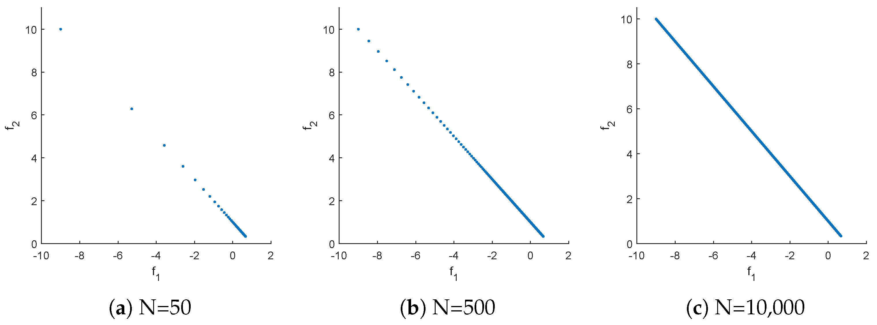
Figure 2.
Representation of the Pareto front of MOP (4) together with the two hypothetical outcomes A and B.
Figure 2.
Representation of the Pareto front of MOP (4) together with the two hypothetical outcomes A and B.
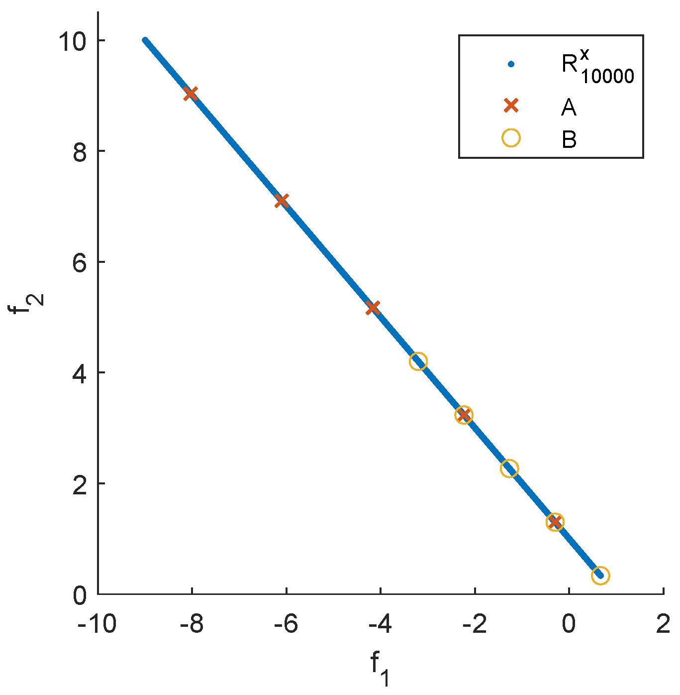
Figure 7.
Filling with (a) and without (b) component detection for ZDT3. Note that points not in the PF are included if the component detection step is omitted (b).
Figure 7.
Filling with (a) and without (b) component detection for ZDT3. Note that points not in the PF are included if the component detection step is omitted (b).
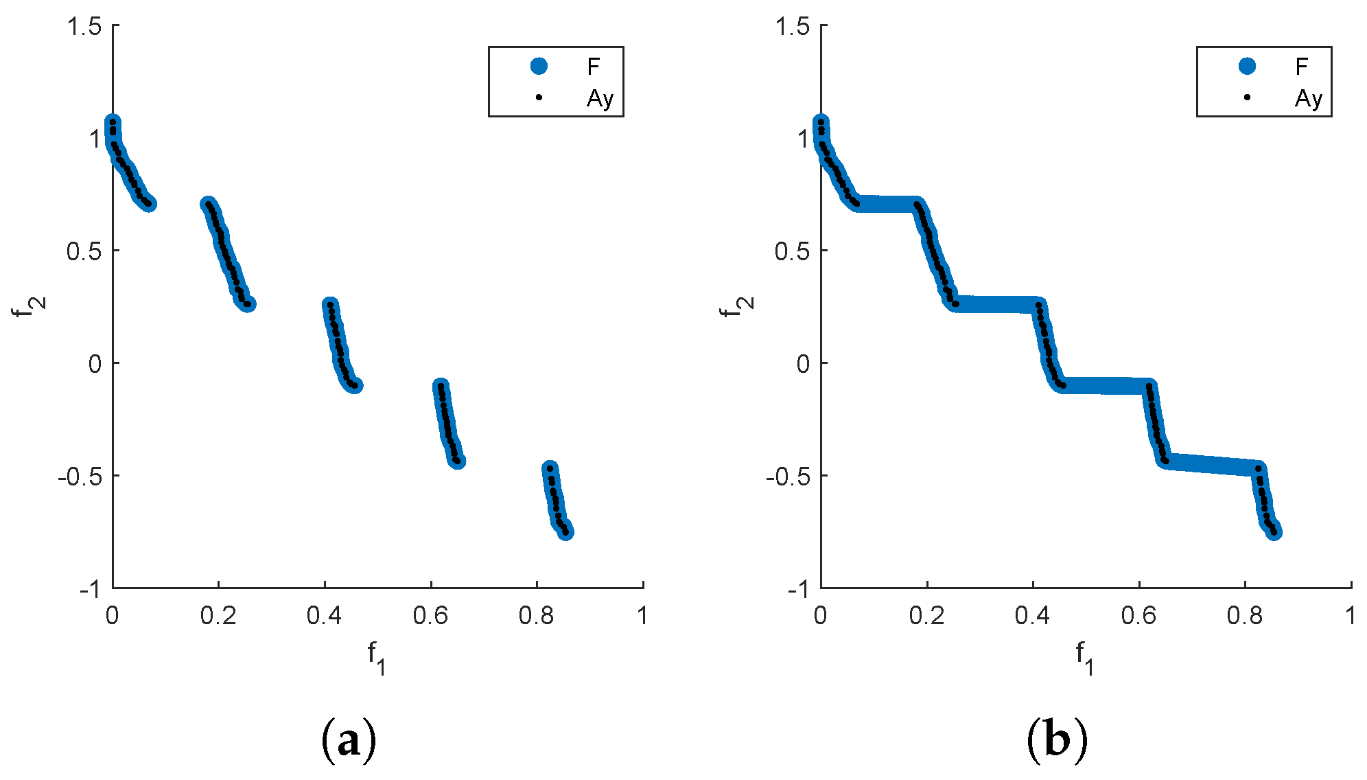
Figure 8.
RSG process for ZDT3. The starting set is taken from PlatEMO. We set .
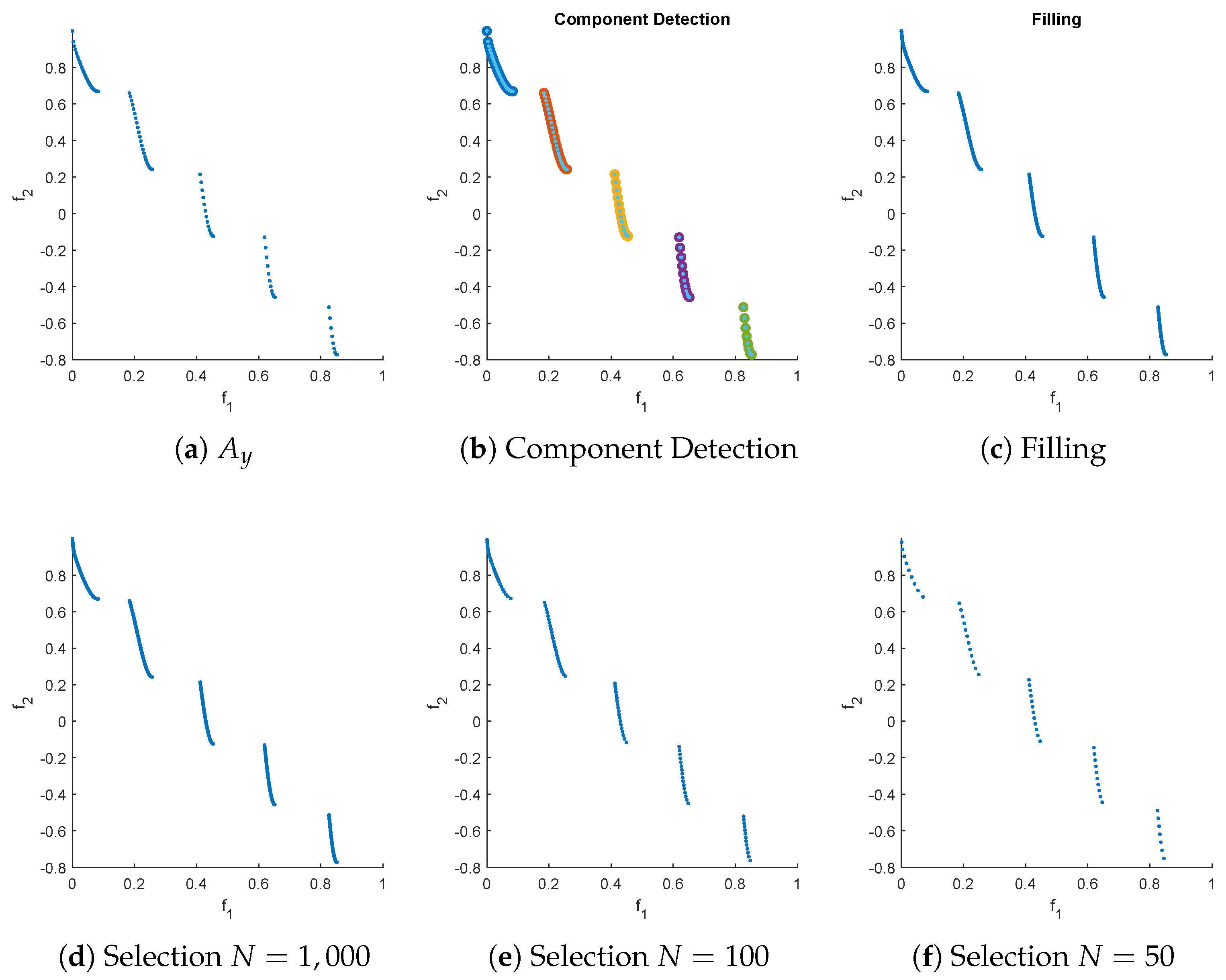
Figure 9.
RSG process for DTLZ7. The starting set is taken from Pymoo. We set . Figure (l) shows the result of RSG with over the same range for all variables, displaying uniformity in the solution.
Figure 9.
RSG process for DTLZ7. The starting set is taken from Pymoo. We set . Figure (l) shows the result of RSG with over the same range for all variables, displaying uniformity in the solution.
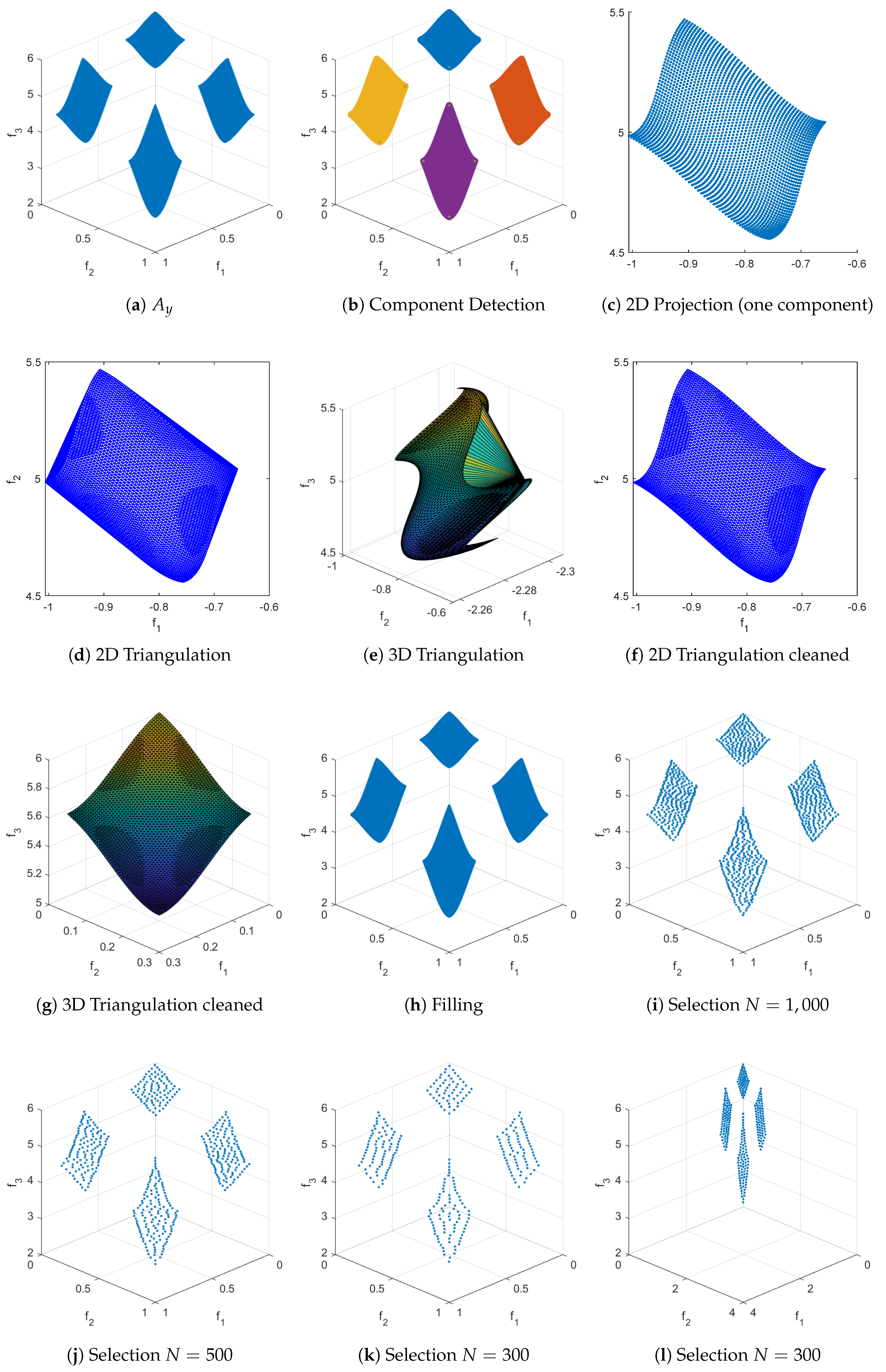
Figure 10.
RSG process for WFG2. The starting set is obtained using the PT and a non-dominance test. We set .
Figure 10.
RSG process for WFG2. The starting set is obtained using the PT and a non-dominance test. We set .
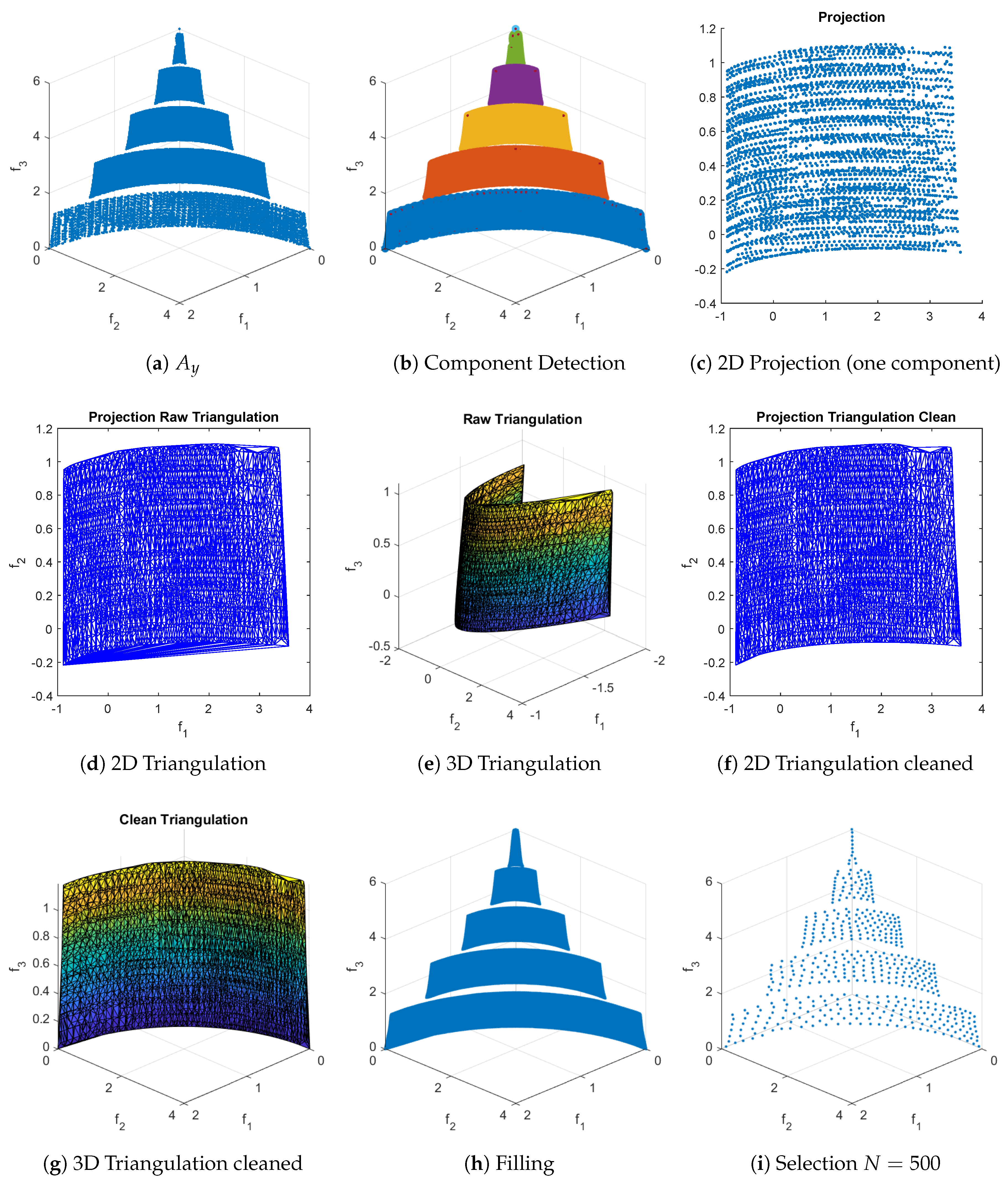
Figure 11.
RSG process for CONV3. The starting set is obtained by sampling 100,000 points uniformly at random near the PS and then applying a nondominance test. We set .
Figure 11.
RSG process for CONV3. The starting set is obtained by sampling 100,000 points uniformly at random near the PS and then applying a nondominance test. We set .
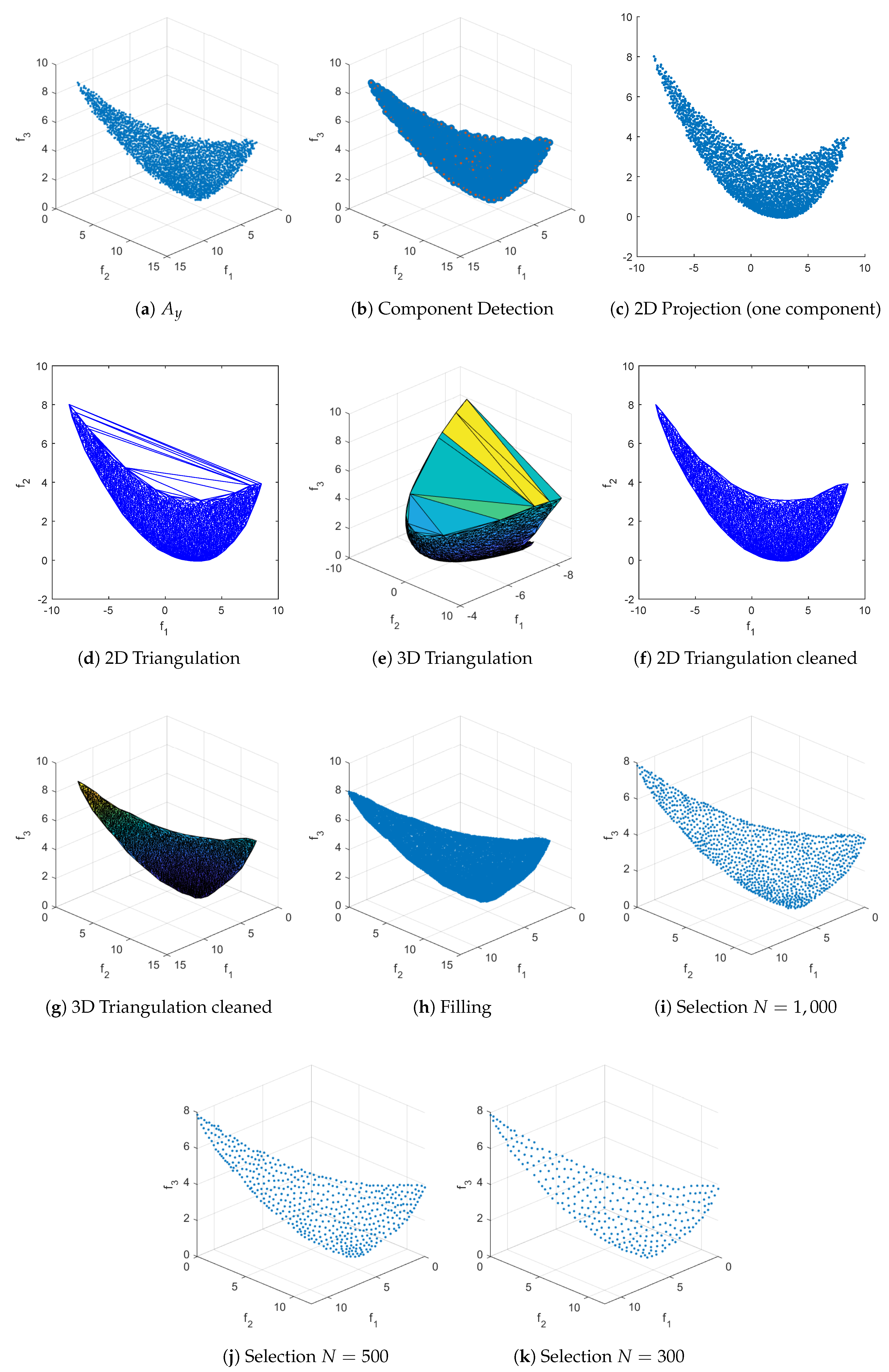
Figure 12.
RSG process for CONV3-4. The starting set is obtained by sampling 100,000 points uniformly at random near the PS and then applying a non-dominance test. We set .
Figure 12.
RSG process for CONV3-4. The starting set is obtained by sampling 100,000 points uniformly at random near the PS and then applying a non-dominance test. We set .
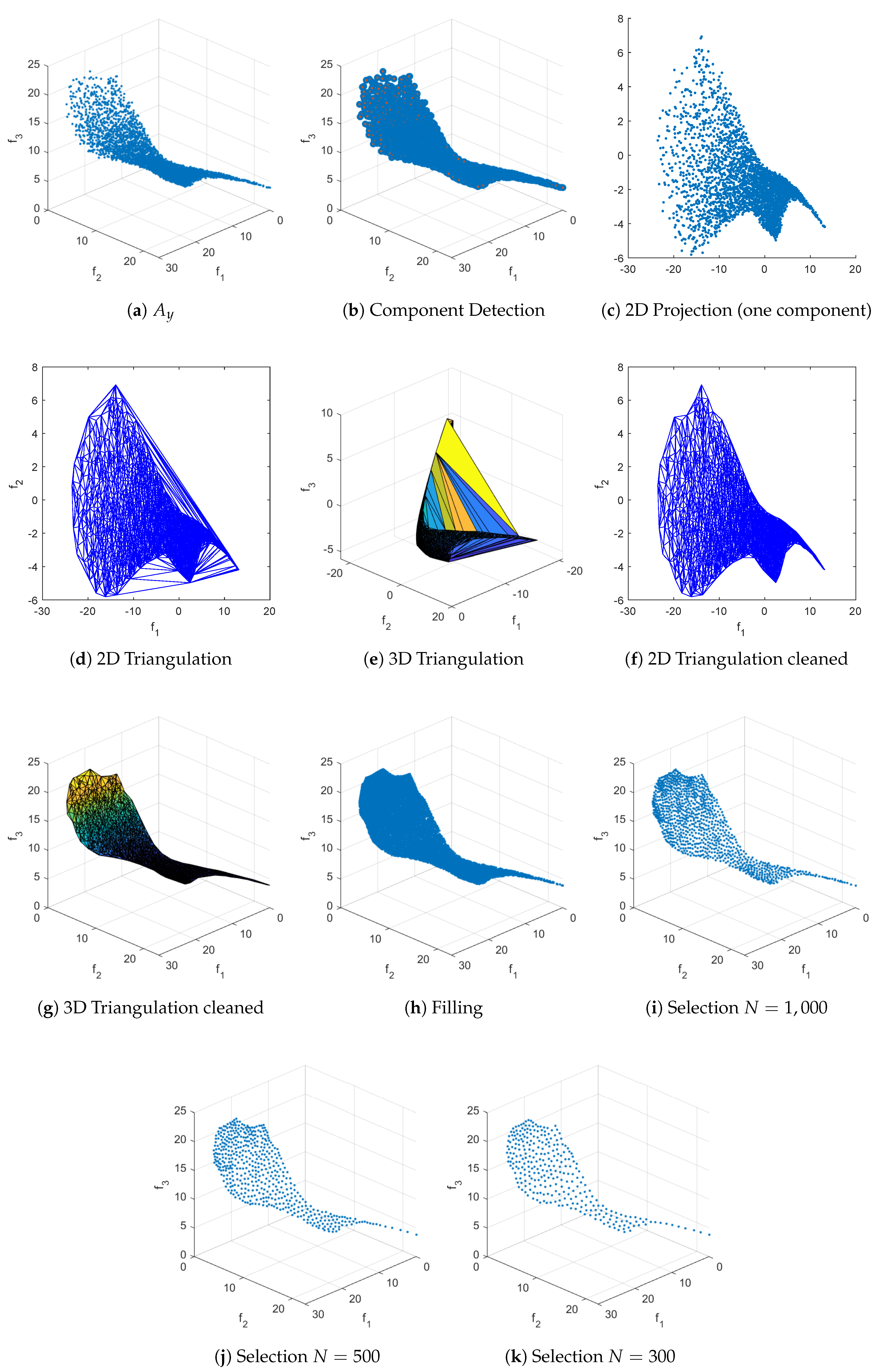
Figure 13.
RSG process for CONV4-2F. The starting set is obtained by merging the final populations from 30 independent runs of NSGA-III, each run consisting of 400 generations with a population size of 500, and then applying a non-dominance test to the merged set. We set .
Figure 13.
RSG process for CONV4-2F. The starting set is obtained by merging the final populations from 30 independent runs of NSGA-III, each run consisting of 400 generations with a population size of 500, and then applying a non-dominance test to the merged set. We set .
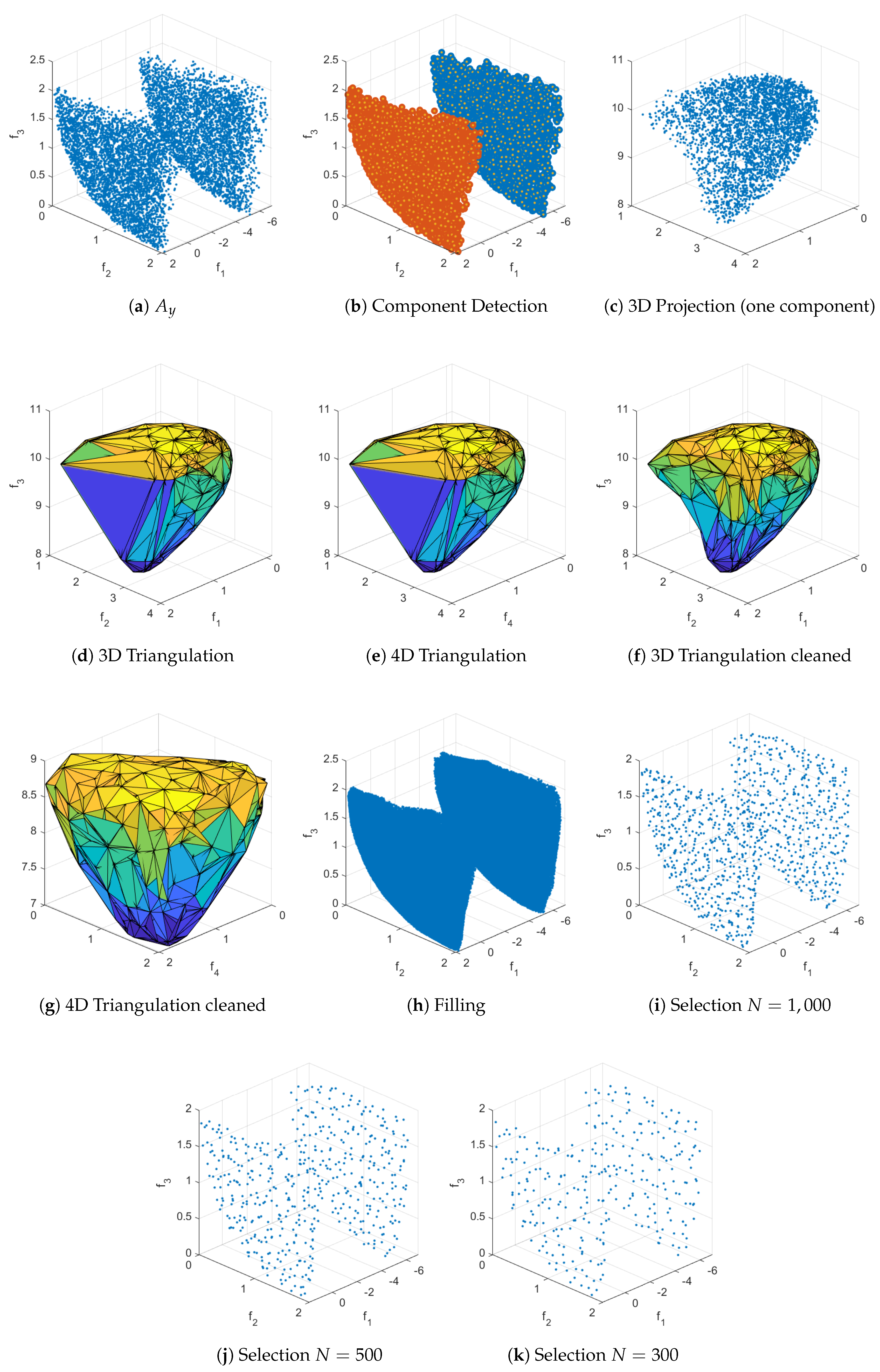
Figure 14.
The first part of the comparisons between RSG (first column), PlatEMO (second column), Pymoo (third column), and the filling step F of RSG (fourth column) are shown. A reference set of size 100 was used for bi-objective problems and 300 for three-objective problems. For bi-objective problems, all methods produced exactly 100 points. However, for three-objective problems, PlatEMO and Pymoo do not always yield exactly 300 points—for example, PlatEMO in WFG1, WFG2, and DTLZ7, and Pymoo in WFG1, WFG2, DTLZ7, CDTLZ2, and C2-DTLZ2, the last two being unobtainable (as far as the authors could determine) in Pymoo.
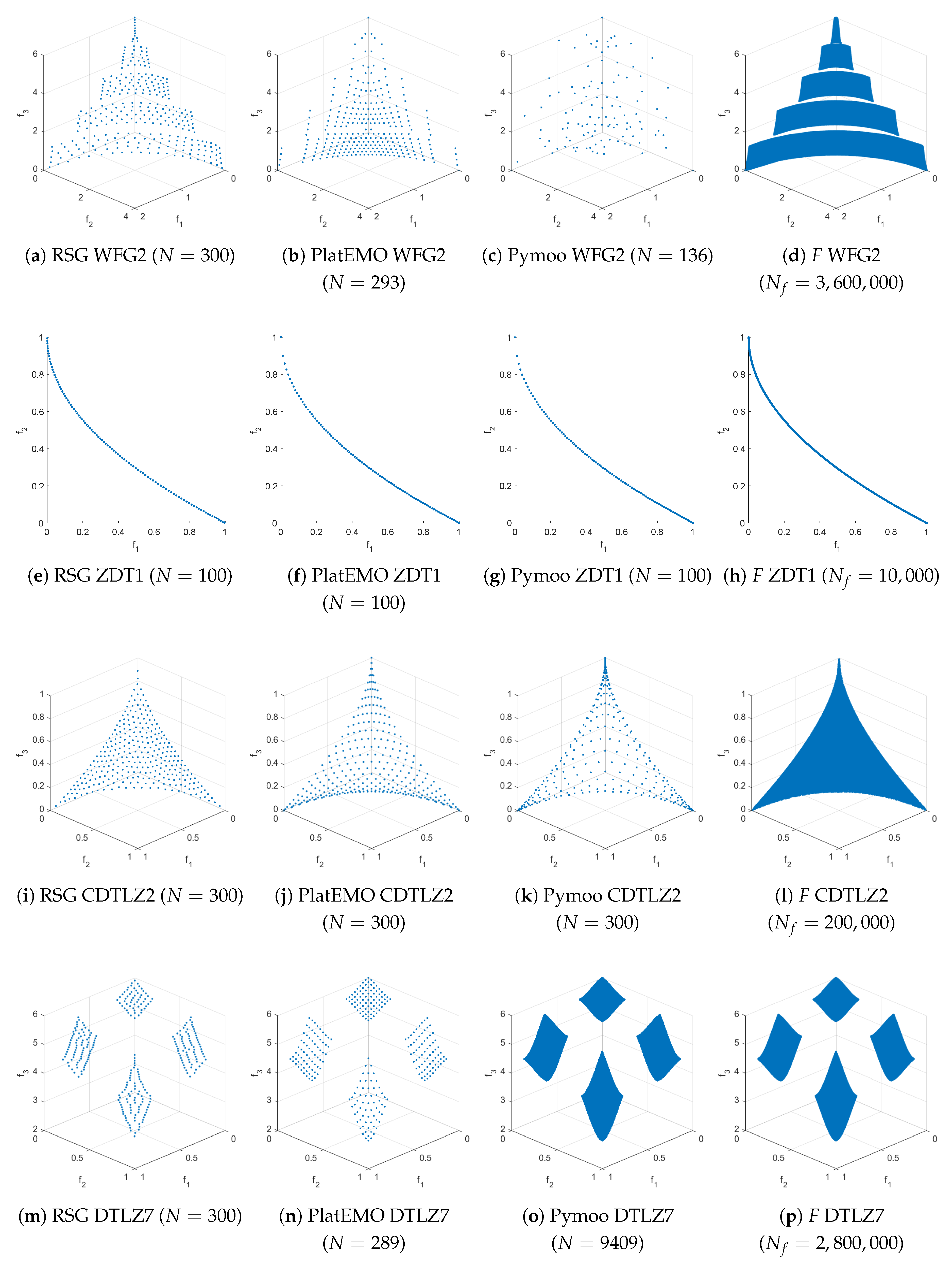
Figure 15.
The second part of the comparisons between RSG (first column), PlatEMO (second column), Pymoo (third column), and the filling step F of RSG (fourth column) are shown. A reference set of size 100 was used for bi-objective problems and 300 for three-objective problems. For bi-objective problems, all methods produced exactly 100 points. However, for three-objective problems, PlatEMO and Pymoo do not always yield exactly 300 points—for example, PlatEMO in WFG1, WFG2, and DTLZ7, and Pymoo in WFG1, WFG2, DTLZ7, CDTLZ2, and C2-DTLZ2, the last two being unobtainable (as far as the authors could determine) in Pymoo.
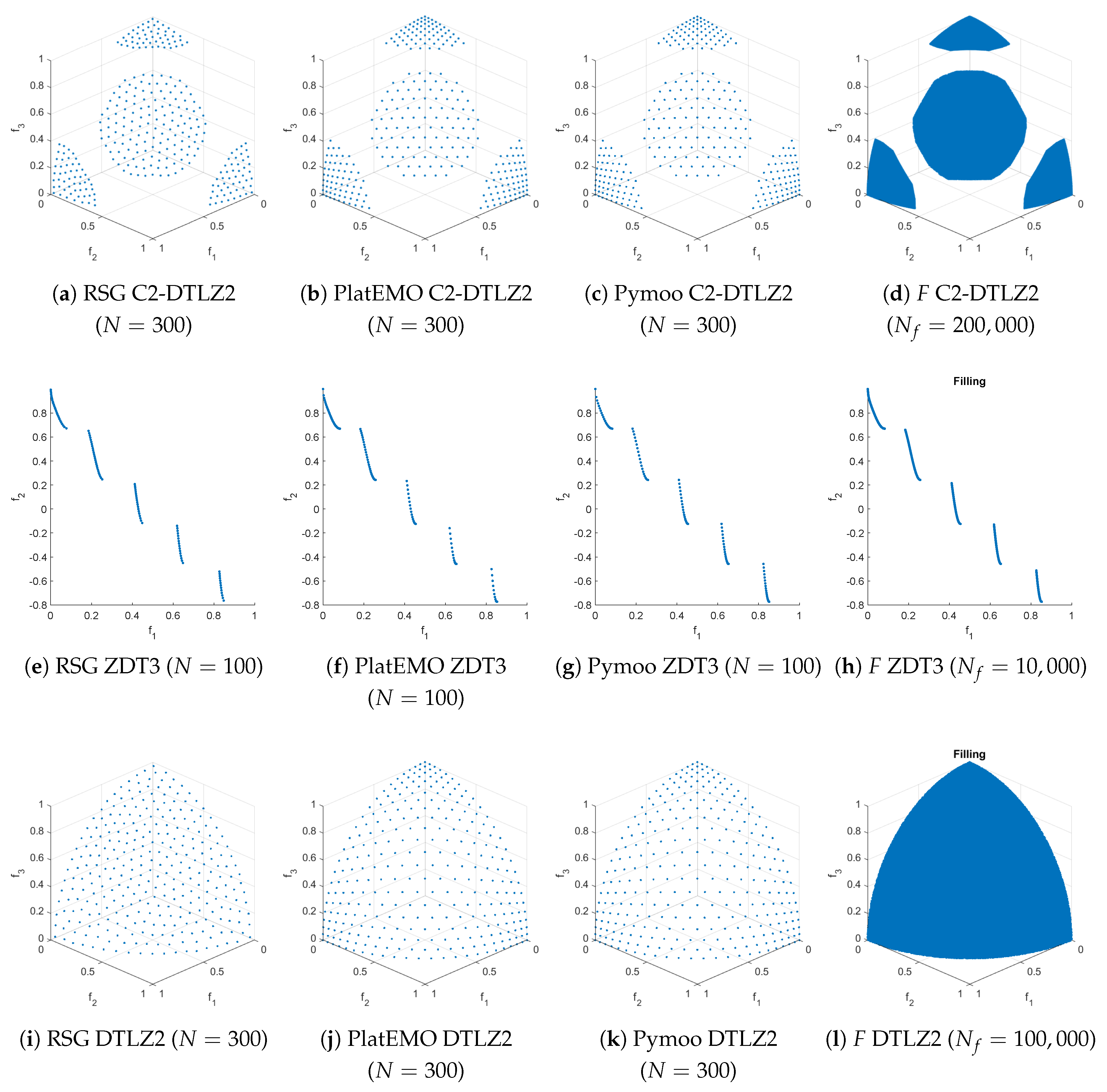

Table 1.
Indicator values for different indicators, the outcomes , and the representations of the Pareto front.
Table 1.
Indicator values for different indicators, the outcomes , and the representations of the Pareto front.
| 0.5118 | 0.7384 | 0.9084 | 0.9873 | 0.6423 | 0.9084 | 0.9873 | 1.3671 | |
| 0.0698 | 0.1002 | 0.4522 | 1.0744 | 0.3198 | 0.4522 | 1.0744 | 8.2024 | |
| 0.0684 | 0.0684 | 0.6835 | 0.7883 | 0.4833 | 0.6835 | 0.7883 | 1.2987 | |
| 0.0684 | 0.0684 | 2.5974 | 3.6765 | 1.8367 | 2.5974 | 3.6765 | 8.1341 | |
| 0.0028 | 0.0032 | 0.8968 | 0.9776 | 0.6341 | 0.8968 | 0.9776 | 1.3671 | |
| 0.0008 | 0.0010 | 0.4117 | 0.8792 | 0.2911 | 0.4117 | 0.8792 | 8.2024 | |
| 0.0007 | 0.0007 | 0.6835 | 0.7893 | 0.4833 | 0.6835 | 0.7893 | 1.3664 | |
| 0.0007 | 0.0007 | 2.5974 | 3.6767 | 1.8367 | 2.5974 | 3.6767 | 8.2018 |
Disclaimer/Publisher’s Note: The statements, opinions and data contained in all publications are solely those of the individual author(s) and contributor(s) and not of MDPI and/or the editor(s). MDPI and/or the editor(s) disclaim responsibility for any injury to people or property resulting from any ideas, methods, instructions or products referred to in the content. |
© 2025 by the authors. Licensee MDPI, Basel, Switzerland. This article is an open access article distributed under the terms and conditions of the Creative Commons Attribution (CC BY) license (http://creativecommons.org/licenses/by/4.0/).
Copyright: This open access article is published under a Creative Commons CC BY 4.0 license, which permit the free download, distribution, and reuse, provided that the author and preprint are cited in any reuse.


