
Submitted:
28 April 2025
Posted:
29 April 2025
You are already at the latest version
Abstract
To address the issues of uneven initial distribution and limited search accuracy in the traditional Divergent Quantum-inspired Differential Search (DCS) algorithm, a hybrid multi-strategy variant, termed DQDCS, is proposed. This improved version overcomes these limitations by integrating the refined set strategy and clustering process for population initialization, along with the Double Q-learning model to balance exploration and exploitation This enhanced version replaces the conventional pseudo-random initialization with a refined set generated through a clustering process, thereby significantly improving population diversity. A novel position update mechanism is introduced based on the original Equation, enabling individuals to effectively escape from local optima during the iteration process. Additionally, the Tables Reinforcement Learning model (Double Q-learning model) is integrated into the original algorithm to balance the probabilities between exploration and exploitation, thereby accelerating the convergence towards the global optimum. The effectiveness of each enhancement is validated through ablation studies, and the Wilcoxon rank-sum test is employed to assess the statistical significance of performance differences between DQDCS and other classical algorithms. Benchmark simulations are conducted using the CEC2019 and CEC2022 test functions, as well as two well-known constrained engineering design problems. The comparison includes both recent state-of-the-art algorithms and improved optimization methods. Simulation results demonstrate that the incorporation of the refined set and clustering process, along with the Tables Reinforcement Learning model (Double Q-learning model) mechanism, leads to superior convergence speed and higher optimization precision.
Keywords:
Differentiated Creative Search algorithm
; Refined Set
; Clustering Process
; Double Q-learning
; Mechanical Optimization
1. Introduction
Optimization theory and its practical applications are undergoing unprecedented transformation in contemporary industrial practice, with their core value lying in the targeted enhancement of key system performance indicators. Driven by the continuous expansion of engineering frontiers and the rapid advancements in computational science, classical optimization paradigms—such as Newton’s method and gradient descent—have increasingly revealed their limitations [1,2,3]. Applied to modern engineering problems with high dimensionality and strong nonlinearity, these methods often face exponential time complexity, making exact solutions practically infeasible. This practical challenge has catalyzed the vigorous development of metaheuristic optimization techniques. These algorithms, inspired by natural phenomena or social behavior [4,5], offer promising alternatives by delivering global or high-accuracy approximate solutions under acceptable computational costs. The balance between solution quality and computational efficiency makes modern metaheuristic algorithms—such as Genetic Algorithms (GA) [6], Particle Swarm Optimization (PSO) [7], and Ant Colony Optimization (ACO) [8]—powerful tools with wide-ranging applicability. These methods have demonstrated exceptional performance in solving complex optimization problems across various interdisciplinary domains, including intelligent manufacturing, logistics scheduling, and financial modeling [9,10,11].
As a vital branch of metaheuristic algorithms, swarm intelligence optimization techniques have attracted increasing attention in the academic community in recent years. These algorithms emulate the cooperative behavior of biological populations—such as the flock migration model in Particle Swarm Optimization (PSO), the mating behavior pattern in Butterfly Optimization Algorithm (BOA) [12], and the deep-sea migration strategy in the Salp Swarm Algorithm (SALP) [13]—demonstrating distinctive computational advantages. Their simple and intuitive structural design, rapid convergence, and multimodal optimization capabilities enable excellent adaptability in solving complex, nonlinear, and high-dimensional engineering optimization problems. Notably, bio-inspired optimization paradigms are undergoing continuous innovation. Modern engineering design methodologies have accelerated the iterative process through parallel search mechanisms and have adopted dynamic balance strategies to coordinate exploration and exploitation. These approaches have delivered significant application value in improving mechanical system performance, reducing operational costs, and optimizing resource allocation efficiency. For instance, Houssein et al. [14] proposed a dimension learning-enhanced equilibrium optimizer that constructs multi-level feature interaction mechanisms, significantly improving the lesion segmentation accuracy of COVID-19 lung CT images, particularly in low-contrast regions. Alkayem et al. [15] developed an adaptive pseudo-inverse stochastic fractal search algorithm that employs intelligent dimensionality reduction strategies within the solution space, enabling robust detection of subtle defects in complex steel structure damage assessments and greatly enhancing diagnostic reliability. Abdollahzadeh et al. [16] introduced the Panthera Optimization (PO) algorithm, which simulates jaguar-inspired intelligent behavior for designing exploration–exploitation mechanisms. By integrating a hyper-heuristic phase transition strategy, the algorithm adaptively balances optimization stages according to problem characteristics, thereby substantially improving the capability to solve complex optimization problems. Liu et al. [17] integrated the Q-learning mechanism from reinforcement learning to dynamically hybridize the Aquila Optimizer (AO) with the Improved Arithmetic Optimization Algorithm (IAOA). By reconstructing the mathematical acceleration function, they achieved a better balance between global search and local exploitation, while optimizing the reward model to enhance decision-making efficiency. Zhu et al. [18] combined the global exploration capability of the Black-Winged Kite Algorithm (KA), the local optimization strength of Particle Swarm Optimization (PSO), and the mutation strategy of Differential Evolution (DE) to balance search abilities, effectively preventing premature convergence and significantly improving both the convergence speed and solution accuracy in high-dimensional optimization problems. However, with the increasing complexity of engineering optimization tasks—characterized by multi-constraint coupling and high-dimensional nonlinearity—current swarm intelligence algorithms have begun to exhibit theoretical limitations when handling non-convex solution spaces and adapting to dynamic environments. In particular, for complex system designs involving strong time-varying properties and multi-objective conflicts, challenges arise in ensuring convergence stability and maintaining well-distributed solution sets.
The Differential Creative Search (DCS) algorithm [19] represents a cutting-edge advancement in the field of metaheuristic optimization. This algorithm introduces an innovative multi-stage co-evolution framework, in which a heterogeneous knowledge transfer mechanism dynamically integrates population experience, while a dynamic solution space reconstruction strategy enhances adaptability to complex optimization problems. DCS demonstrates strong global convergence performance in tackling high-dimensional, non-convex, and multimodal engineering optimization tasks. Liu et al. [20] proposed a hybrid approach incorporating an opposition-based learning strategy along with an adaptive reset mechanism that balances fitness and distance. This design encourages low-performance individuals to migrate toward the vicinity of the optimal solution, thereby facilitating the exploration of promising regions in the search space. Cai et al. [21] improved the shortcomings of DCS algorithm through collaborative development mechanism and population evaluation strategy.However, DCS still suffers from limitations in terms of solution distribution bias and insufficient local convergence precision during iterations, which restrict its ability to effectively explore the boundary regions of the search space and identify the global optimum. To address these challenges, we propose an improved initialization strategy that integrates a refined set with a clustering process to enhance the diversity of the initial population. Furthermore, we incorporate a Double Q-learning strategy using dual Q-tables, enabling a more effective balance between exploration and exploitation. This balance empowers the algorithm to explore unknown regions in complex environments more effectively, thereby reducing the risk of premature convergence to local optima.
The main contributions of the proposed algorithm in this study are summarized as follows:
(1) A novel algorithm is developed by integrating a refined set, a clustering process, and a Double Q-learning strategy into the Differential Creative Search (DCS) framework. Ablation studies are conducted to verify that each of these strategies contributes positively to the performance enhancement of the DCS algorithm.
(2) The proposed DQDCS algorithm is benchmarked against ten state-of-the-art algorithms on the CEC2019 and CEC2022 test suites. Extensive simulations demonstrate the superior performance of DQDCS. Its improvements are visualized through convergence curves and box plots, and further validated by the Wilcoxon rank-sum test to confirm its overall effectiveness.
(3) The DQDCS algorithm is applied to two real-world constrained engineering design problems: the design of hydrostatic thrust bearings and the Synchronous Optimal Pulse Width Modulation (SOPWM) problem in three-level inverters. In both cases, the goal is to minimize the objective function under complex constraints. The results show that DQDCS is particularly suitable for solving practical engineering optimization problems.
The remainder of this study is organized as follows. Section 2 introduces the fundamentals of the Differential Creative Search (DCS) algorithm. Section 3 elaborates on the three enhancement strategies incorporated into DQDCS. Section 4 reports the experimental comparisons between DQDCS and other algorithms on the CEC2019 and CEC2022 benchmarks. Section 5 presents the application of DQDCS to practical engineering problems and offers a comprehensive analysis of the results. Finally, Section 6 concludes the study.
2. Differentiated Creative Search Algorithm Thoughts and Process
The Differentiated Creative Search (DCS) algorithm is a swarm intelligence-based optimization method, whose core framework integrates Differentiated Knowledge Acquisition (DKA) and Creative Realism (CR). A dual-strategy mechanism is employed to balance divergent and convergent thinking. In this framework, high-performing individuals adopt a divergent thinking strategy, utilizing existing knowledge and creative reasoning to conduct global exploration guided by the Linnik distribution. In contrast, the remaining individuals adopt a convergent thinking strategy, integrating feedback from both the team leader and peer members to perform local exploitation. This process involves local optimization informed by both elite and randomly selected individuals. The overall procedure of the DCS algorithm is summarized as follows.
2.1. Initialization
The initial population X is randomly generated, with each individual represented as a random solution.
satisfying the Equation (1).
where and represent the lower and upper bounds of the d-th dimension, respectively, and follows a uniform distribution on the interval .
2.2. Differentiated Knowledge Acquisition
Differentiated Knowledge Acquisition (DKA) emphasizes the rate at which new knowledge is acquired, exerting differential effects on individual agents. These effects are primarily manifested through the modification of the individual’s existing knowledge attributes or dimensional components. The parameter denotes the quantified knowledge acquisition rate of the i-th individual at iteration t, as defined in Equation (2).
In Equation (2), represents the coefficient associated with variable for the individual at the t-th iteration, and is calculated using Equation (3). Here, NP denotes the population size, and indicates the rank of the i-th individual at the beginning of iteration t. The influence of the DKA process on each component of is described in Equation (4), where denotes an integer uniformly selected from the set , and D represents the dimensionality of the problem.
2.3. Convergent Thinking
The strategy for low-performing individuals leverages the knowledge base of high performers and incorporates the stochastic contributions of two randomly selected team members into the solution proposed by the current individual. This process is described by Equation (5), where F denotes the inertia weight and represents the global best solution in the current population.
draws upon convergent thinking by integrating the information provided by team members and , thereby refining the knowledge of the team leader, , as described by Equation (6). Here, the coefficient governs the extent to which peer influence shapes an individual’s social cognition within the team environment. It reflects the degree to which team dynamics affect individual perspectives. The value of decreases over time, as defined in Equation (7), where NFET and NFEmax denote the number of function evaluations in the current iteration and the maximum allowable number of function evaluations, respectively.
Two random individuals, and , are selected, and a new candidate solution is generated by incorporating the best individual with stochastic components, as defined in Equation (8).
2.4. Divergent Thinking
A random individual is selected, and a new candidate solution is generated using the Linnik distribution, as defined in Equation (9), where denotes a random variable drawn from the Linnik distribution with parameters and .
2.5. Team Diversification
As the team continues to evolve, it generates increasingly diverse ideas. To maintain diversity and adaptability, the DCS algorithm replaces underperforming members with newly generated individuals. The equation used to generate new individuals is provided in Equation (10).
2.6. Offspring Population
For each individual , a trial solution is generated. The decision to retain or replace the original solution is based on a comparison of their fitness values. If the trial solution exhibits superior fitness, it replaces the original solution ; otherwise, the original solution is retained. This process is formulated in Equation (11).
In each iteration, all individuals in the newly generated population are evaluated, and the global best solution is subsequently updated. This process is formally defined in Equation (12).
Algorithm 1 outlines the detailed steps of the DCS algorithm as described above.
| Algorithm 1 Particle swarm optimization |
| Step 1: Random Initialization of the Population The initial population is generated randomly to ensure diversity in the solution space. Step 2: Fitness Evaluation The fitness of each individual is evaluated by computing its objective function value, which reflects the individual’s performance on the optimization problem. Step 3: Determination of the Number of High-Performance Individuals The number of top-performing individuals is determined based on a predefined proportion of the population. Step 4: Initialization of Iteration Counter and Parameters Set the iteration counter t=1, the number of function evaluations NFE=0, and the probability of population migration to 0.5. Step 5: Main Optimization Loop Continue the optimization process while NFE < NFEmax, repeating the position updating and fitness evaluation steps. |
3. Hybrid Multi-Strategy Differentiated Creative Search Algorithm
Firstly, the DCS algorithm initializes the population using pseudo-random numbers, which results in limited population diversity and a lack of target-oriented search in the early stages, thereby reducing optimization efficiency. Secondly, the algorithm relies heavily on the best-performing individual during position updates, making it susceptible to premature convergence and hindering its ability to escape local optima. These issues ultimately lead to reduced optimization accuracy and a slower convergence rate.
To address these limitations, targeted strategies are introduced to enhance the algorithm’s overall performance. Previous studies have shown that the diversity of the initial population significantly influences the algorithm’s ability to converge rapidly and accurately. A higher degree of initial diversity allows the algorithm to explore a broader solution space during the search process, thereby increasing the likelihood of identifying the global optimum.
To improve population diversity, generate higher-quality initial solutions, and effectively overcome the limitations of the basic DCS algorithm, a refined set strategy and clustering strategy are incorporated during the population initialization phase. Although the DCS algorithm enhances global exploration through its “creativity” mechanism, it lacks sufficient flexibility in dynamic environments, such as path planning with moving obstacles for UAVs (Unmanned Aerial Vehicles) or real-time demand changes in industrial scheduling.
The incorporation of Double Q-learning allows the algorithm to interact continuously with the environment, facilitating real-time perception and autonomous decision-making. This enables the DCS algorithm to adapt its search strategy more precisely under dynamic conditions, thereby maintaining high operational efficiency. Furthermore, the learning capability of Double Q-learning enhances the algorithm’s generalization ability, enabling robust performance in unseen scenarios and increasing the practical value of intelligent optimization techniques.
3.1. Refined Set Initialization
Compared to traditional pseudo-random initialization, the refined set strategy achieves a more uniform distribution of the population across the search space through a carefully designed sampling method. This uniformity reduces the likelihood of the algorithm becoming trapped in local optima during the early stages of optimization. By promoting a broader distribution of individuals, the algorithm gains increased opportunities to explore diverse regions and identify superior solutions.
The mathematical formulation of the refined set strategy is presented in Equations (13) and (14), where L and U represent the lower and upper bounds of the d-th dimension, respectively, and i indicates the index of the i-th individual. The parameter p denotes the smallest prime number that satisfies specific conditions, and refers to the result of the modulo operation applied to with respect to p.
3.2. Clustering Process
After the population is generated using the refined set strategy, a clustering algorithm is applied for further enhancement. In this study, the k-means clustering method is adopted to allow the DCS algorithm to focus on salient features during the learning phase while minimizing the impact of low-quality data. This process improves the algorithm’s generalization ability on unseen data, thereby increasing its robustness and stability in practical applications. The detailed implementation steps are presented as follows.
- (1)
- Select the Cluster Centers
Randomly select k points as the initial cluster centers where .
- (2)
- Calculate the distance and assign individuals.
For each individual in the population, the Euclidean distance between and each cluster center is calculated. The individual is then assigned to the cluster corresponding to the nearest cluster center. This is specifically expressed by Equation (15).
- (3)
- Update the cluster centers.
For each cluster, the cluster center is recalculated. Let the set of individuals in the j-th cluster be denoted as . The new cluster center is computed as the mean of the individuals in , where denotes the number of individuals in the set .
- (4)
- Iterative process.
Repeat steps 2 and 3 until the cluster centers no longer undergo significant changes.
- (5)
- Density-based uniform selection.
Calculate the local density of each individual , denoted as where is the truncation distance used in the density calculation. Individuals with moderate density are selected, and the final initialized population is given by Equation (16).
3.3. Double Q Tables Reinforcement Learning Model (Double Q-Learning Model)
The Q-learning model consists of five fundamental components: the agent, environment, action, state, and reward. Its operational procedure can be succinctly described as a cyclical interaction of state transition, action selection mechanism, and reward feedback. In traditional Q-learning, a single Q-table is employed to store the estimated values of state–action pairs. However, this approach often suffers from issues such as overestimation bias and limited exploration capacity. To mitigate these limitations, Double Q-learning introduces two independent Q-tables, each of which is updated independently. This dual-table framework significantly reduces the estimation bias inherent in the single-table approach and enables a more balanced, robust evaluation of the learned policy.
Let denote the set of environment states and represent the set of actions that the agent can execute. In each iteration, the agent occupies a certain state and selects an action to perform. After executing the action, the environment provides a reward and a new state . The reward is computed according to Equation (17), where denotes the solution at the new position, and represents the solution at the current position. Upon receiving this information, the agent evaluates the expected value for each possible action.
In Double Q-learning, either or is selected for updating with equal probability. The update equations are provided in Equations (18) and (19). In the equations, represents the state of the agent, denotes the action executed by the agent, is the immediate reward obtained by the agent after executing the action, and is the discount factor, which penalizes future rewards. When , Double Q-learning considers only the current reward; when , it prioritizes long-term rewards, is the learning rate, typically within the interval . Double Q-learning maintains two Q-tables, traditional Q-learning, but with distinct update logic. Figure 1 simplified illustration example of the operational process of Double Q-learning. The agent alternates between updating the two Q-tables and combines information from both when selecting actions, thereby reducing estimation bias and enhancing policy robustness.
In the DCS algorithm, the last individual is considered inefficient and updated using random initialization, which often results in low-quality solutions. To address this issue, Double Q-learning introduces two independent Q-tables and employs a dual Q-table mechanism to improve solution quality. This separation makes the calculation of target Q-values more reliable, helping to reduce estimation bias.
3.4. Ablation Experiment
To evaluate the effectiveness of the proposed strategies, four representative test functions from the CEC2019 benchmark suite were selected. The performance of the refined set strategy, the clustering process strategy, their combination, and the Double Q-learning strategy was systematically compared. Each algorithm was executed for 500 iterations across 30 independent runs. Specifically, D1 adopts the refined set strategy, D2 employs the clustering process strategy, D3 integrates both the refined set and clustering process strategies, and D4 incorporates the Double Q-learning mechanism. The corresponding results are summarized in Table 1. Experimental results demonstrate that population initialization using the combined refined set and clustering process significantly enhances the algorithm’s capability to approach the global optimum. Moreover, the D4 variant, augmented with the Double Q-learning strategy, achieves the best overall fitness across all test functions.

Table 1.
Ablation experiment results for each strategy.
| DCS | D1 | D2 | D3 | D4 | |
| F2 | 3.4322 | 3.322 | 3.2916 | 3.2725 | 3.1517 |
| F5 | 1.0297 | 1.0409 | 1.0297 | 1.017 | 1.0008 |
| F8 | 3.0423 | 3.0227 | 3.0233 | 2.8924 | 2.447 |
| F10 | 1.0044 | 1.0037 | 1 | 1.0035 | 1.0001 |
| DCS | D1 | D2 | D3 | D4 | |
| F2 | 3.4322 | 3.322 | 3.2916 | 3.2725 | 3.1517 |
| F5 | 1.0297 | 1.0409 | 1.0297 | 1.017 | 1.0008 |
| F8 | 3.0423 | 3.0227 | 3.0233 | 2.8924 | 2.447 |
| F10 | 1.0044 | 1.0037 | 1 | 1.0035 | 1.0001 |
3.5. Hybrid Multi-Strategy DQDCS Algorithm
The DQDCS algorithm integrates both the refined-point set strategy and a clustering-based approach, and further incorporates a Double Q-learning model to construct a multi-strategy hybrid optimization framework. The refined-point set is generated through mathematically guided sampling techniques to ensure a more uniform distribution of individuals across the search space, thereby replacing conventional pseudo-random initialization methods. Such a distribution promotes broader coverage of the solution space and mitigates early-stage search blind spots. A high-quality initial population enhances the algorithm’s ability to converge more reliably toward optimal solutions and reduces performance fluctuations caused by poor initial positioning.
In contrast to purely random initialization, the refined-point set strategy employs structured sampling to diminish the randomness-induced variability in the initial population, thereby improving the algorithm’s robustness. Moreover, this strategy can be tailored to the specific characteristics of the optimization problem; for example, in constrained optimization scenarios, it helps ensure that the initial population satisfies constraint conditions, thus avoiding infeasible solutions and enhancing overall algorithmic stability.
The clustering strategy divides the population into multiple subgroups, with each subgroup representing distinct regions or features of the search space. This structural partitioning aids in preserving diverse solution patterns throughout the optimization process, thereby reducing the risk of premature convergence to local optima. By maintaining diversity and promoting exploration, the algorithm is better positioned to locate the global optimum efficiently.
By integrating the probability distributions and maximum values derived from two independent Q-tables, the Double Q-learning mechanism enables more balanced action selection between exploration and exploitation. Within the DQDCS algorithm, this dual-Q-table framework effectively mitigates the estimation bias commonly associated with single Q-table implementations and facilitates more comprehensive policy evaluation, thereby enhancing the algorithm’s global search capability. Specifically, Double Q-learning selects the optimal action based on the current state, which subsequently guides population updates. This approach allows for broader exploration during the early stages of optimization, while gradually shifting toward refined exploitation of promising regions in the later stages. So, the algorithm achieves accelerated convergence without compromising solution quality. The flowchart of the DQDCS algorithm is illustrated in Figure 2.
Algorithm 2 presents the pseudocode of the proposed DQDCS algorithm.
| Algorithm 2: DQDCS algorithm. |
| Initialize the population using Equation (1); Evaluate fitness for all individuals; Determine the refined set via the clustering process; Initialize Q-tables to zero; Set key parameters: exploration threshold pc, golden ratio, η and φ values; while the number of function evaluations (nfe) < max_nfe do Sort the population by fitness; Identify the best solution x_best; Compute λt using Equation (7); for each individual i do Compute ηᵢ and φᵢ using Equations (2)–(3); Determine behavior category (high-, average-, or low-performing); if i is low-performing and rand < pc then Generate a new solution randomly; else if i is high-performing then Select r₁ ≠ i; Update selected dimensions using Equation (8); else // average-performing Select r₁, r₂ ≠ i; Compute ωᵢ; Update selected dimensions using Equation (8); end if Apply reflection-based boundary handling; Evaluate fitness of the new solution; If improved, update position and fitness; Compute reward from fitness change; Update Q₁ using Q₂ for value estimation (Equation 18); Update Q₂ using Q₁ similarly (Equation 19); end for Update the best solution and record convergence data; end while Return best solution, best fitness; |
3.6. Complexity Analysis of the Algorithm
The implementation of the DQDCS algorithm involves certain design challenges, yet it maintains a relatively low computational complexity. The overall complexity is stage-dependent, as each phase—initialization, fitness evaluation, and solution generation—contributes differently to the total computational cost.
In general, the DQDCS algorithm comprises three fundamental procedures: population initialization, fitness evaluation, and generation of new solutions. The main loop iterates for a maximum of Max_iter iterations, and in each iteration, operations are performed for each of the N search agents.
The computational complexity of the initialization phase is O(N), owing to the refined set-based initialization method and clustering process. Additionally, the time complexity for fitness evaluation depends on the complexity of the objective function, denoted as O(F). Therefore, the overall computational complexity of the algorithm can be expressed as O(Max_iter × N × F).
4. Simulation Environment and Result Analysis
In the field of optimization, particularly in the study of evolutionary algorithms and metaheuristic methods, validating the effectiveness of proposed algorithms is of paramount importance, as these approaches are expected to address complex challenges encountered in real-world applications. To assess their performance, standardized test cases or well-established benchmark problems are commonly employed. These benchmark evaluations offer a unified platform for objective comparison, enabling fair and consistent performance assessment across different algorithms and facilitating a rigorous analysis of their strengths and limitations.
The experiments were conducted using MATLAB 2023 on a Windows 11 operating system. The CEC2019 [28] and CEC2022 [29] benchmark functions were employed to evaluate the performance of the DQDCS algorithm. These benchmark functions enable a systematic comparison between DQDCS and other state-of-the-art metaheuristic algorithms, thereby verifying the competitiveness and applicability of the proposed method in solving complex optimization problems. This evaluation framework ensures scientific rigor and provides clear directions for further algorithmic enhancements.
Considering the inherent stochastic nature of metaheuristic algorithms, relying on a single run for each benchmark function may lead to unreliable conclusions. Therefore, multiple simulations were conducted for each algorithm, including the original Differentiated Creative Search algorithm (DCS) [19], the multi-strategy hybrid DQDCS algorithm [20], A Differentiated Creative Search Algorithm with Multi-Strategy Improvement (MSDCS), Chernobyl Disaster Optimizer (CDO) [22], Puma Algorithm [16], Waterwheel Plant Algorithm (WWAP) [24], Sub-Population Improved Grey Wolf Optimizer with Gaussian Mutation and Lévy Flight (SPGWO) [25], the Dung Beetle Optimizer (DBO) [26], Nonlinear Randomly Reuse-Based Mutated Whale Optimization Algorithm (NRRMWOA) [27], and the Adaptive Spiral Flying Sparrow Search Algorithm (ASFSSA) [23]. The detailed experimental results are presented as follows.
4.1. The CEC2019 Benchmark Functions Are Employed for Performance Evaluation
The CEC2019 benchmark functions are specifically designed to evaluate and compare the performance of optimization algorithms. It encompasses a diverse set of challenging optimization problems, including multimodal, high-dimensional, and dynamic characteristics, thereby closely simulating real-world complexities. Given the inherent stochastic nature of metaheuristic algorithms, a single run per benchmark function is insufficient to reliably demonstrate an algorithm’s effectiveness. To enhance the reliability and fairness of performance evaluation, each algorithm was independently tested 100 times on each benchmark function, with a maximum of 500 iterations per run.
4.1.1. Optimization Accuracy Analysis
To accurately evaluate and compare the performance on the CEC2019 benchmark functions, the experimental results are summarized in terms of the best, mean, and standard deviation (Std) values. In the result tables, the best mean values, which serve as key performance indicators, are highlighted with underlining. The detailed outcomes are presented in Table 1.
As shown in the statistical results in Table 2, the proposed DQDCS algorithm consistently achieves the best values on all functions from F1 to F10. Moreover, it obtains the best mean performance on F1 and F3–F10 compared to other competing algorithms. In addition, the DQDCS achieves the smallest standard deviation on functions F3, F5, F6, F8, and F9, demonstrating superior robustness. These findings indicate that DQDCS not only offers stable performance but also exhibits highly competitive exploration capability among the compared algorithms.
Table 1.
Experimental results on the CEC2019 benchmark functions.
| Function | Algorithm | Best | Mean | Std |
|---|---|---|---|---|
| F1 | DCS | 1 | 1.1746 | 0.066539 |
| DQDCS | 1 | 1.0129 | 0.017456 | |
| MSDCS | 1.0001 | 54.4005 | 138.3435 | |
| CDO | 1 | 1.2 | 0 | |
| Puma | 1 | 103218.6127 | 227810.8443 | |
| WWPA | 1.6834 | 238.3049 | 583.4071 | |
| SPGWO | 1 | 3656.3391 | 8551.4486 | |
| DBO | 1 | 414533.6708 | 721175.8267 | |
| NRRMWOA | 180.8782 | 785017.9378 | 1311767.1446 | |
| SABO | 1 | 5.7741 | 21.3505 | |
| ASFSSA | 1 | 1 | 0 | |
| F2 | DCS | 3.4322 | 33.4401 | 48.401 |
| DQDCS | 3.1517 | 32.8329 | 49.4357 | |
| MSDCS | 5.1132 | 9.6797 | 4.1544 | |
| CDO | 5 | 5 | 0 | |
| Puma | 4.2328 | 4.7036 | 0.37262 | |
| WWPA | 5.2001 | 8.3147 | 3.6477 | |
| SPGWO | 63.7169 | 259.0299 | 142.4842 | |
| DBO | 4.2752 | 384.2964 | 194.8378 | |
| NRRMWOA | 11.9124 | 721.1422 | 965.2022 | |
| SABO | 4.5993 | 8.7857 | 5.9168 | |
| ASFSSA | 4.2189 | 4.3289 | 0.18135 | |
| F3 | DCS | 2.2424 | 2.9371 | 0.4211 |
| DQDCS | 1.0004 | 2.0439 | 0.2884 | |
| MSDCS | 11.7269 | 12.4015 | 0.34845 | |
| CDO | 4.7096 | 5.8612 | 0.64681 | |
| Puma | 1.4656 | 2.1404 | 0.57859 | |
| WWPA | 8.0688 | 10.1437 | 0.86708 | |
| SPGWO | 2.4504 | 3.2425 | 0.74601 | |
| DBO | 1.4091 | 3.9766 | 1.8562 | |
| NRRMWOA | 1.4106 | 4.9893 | 1.953 | |
| SABO | 5.7387 | 6.9026 | 0.57406 | |
| ASFSSA | 1.0134 | 3.6414 | 1.5732 | |
| F4 | DCS | 5.1848 | 7.2552 | 1.0675 |
| DQDCS | 5.01 | 5.5951 | 1.8712 | |
| MSDCS | 85.6623 | 136.8029 | 21.366 | |
| CDO | 63.5432 | 71.4357 | 5.479 | |
| Puma | 5.9748 | 13.0409 | 5.7055 | |
| WWPA | 116.9494 | 142.2562 | 13.0633 | |
| SPGWO | 4.0021 | 14.8937 | 9.5953 | |
| DBO | 11.0965 | 23.7472 | 8.109 | |
| NRRMWOA | 17.0311 | 43.543 | 18.719 | |
| SABO | 35.1635 | 45.1917 | 7.9818 | |
| ASFSSA | 7.9865 | 41.071 | 29.6237 | |
| F5 | DCS | 1.0297 | 1.0793 | 0.047848 |
| DQDCS | 1.0008 | 1.0577 | 0.034179 | |
| MSDCS | 76.1748 | 153.0113 | 42.5413 | |
| CDO | 53.7219 | 72.8935 | 4.7508 | |
| Puma | 1.0271 | 1.1604 | 0.096242 | |
| WWPA | 122.0759 | 173.3345 | 21.0507 | |
| SPGWO | 1.1723 | 1.5255 | 0.22175 | |
| DBO | 1.0442 | 1.1462 | 0.06739 | |
| NRRMWOA | 1.2785 | 1.5229 | 0.17431 | |
| SABO | 1.7572 | 2.9426 | 0.93688 | |
| ASFSSA | 1.0615 | 1.1646 | 0.072103 | |
| F6 | DCS | 1.0004 | 1.9302 | 1.0947 |
| DQDCS | 1.0029 | 1.4685 | 0.73351 | |
| MSDCS | 9.6249 | 14.1852 | 1.4021 | |
| CDO | 7.8188 | 9.4417 | 0.90669 | |
| Puma | 1.004 | 1.7517 | 0.89464 | |
| WWPA | 11.2646 | 12.8644 | 0.87031 | |
| SPGWO | 1.281 | 2.1444 | 0.92531 | |
| DBO | 2.0546 | 4.6142 | 1.7611 | |
| NRRMWOA | 4.9513 | 7.5365 | 1.5727 | |
| SABO | 2.8428 | 4.748 | 0.97675 | |
| ASFSSA | 1.0009 | 2.6429 | 1.1644 | |
| F7 | DCS | 119.6257 | 591.2146 | 214.4368 |
| DQDCS | 80.447 | 347.2542 | 160.8203 | |
| MSDCS | 1910.947 | 2563.8317 | 271.9363 | |
| CDO | 1174.9817 | 1493.4973 | 180.7765 | |
| Puma | 126.3932 | 605.3863 | 286.0483 | |
| WWPA | 2117.4231 | 2407.1589 | 144.384 | |
| SPGWO | 342.6493 | 736.2504 | 217.0422 | |
| DBO | 417.6764 | 786.1656 | 309.1151 | |
| NRRMWOA | 499.5293 | 1150.2235 | 299.2043 | |
| SABO | 1214.0837 | 1760.7036 | 189.8127 | |
| ASFSSA | 293.3793 | 800.6022 | 282.4334 | |
| F8 | DCS | 3.0423 | 3.5322 | 0.56543 |
| DQDCS | 2.447 | 3.365 | 0.022699 | |
| MSDCS | 4.654 | 5.2571 | 0.0764 | |
| CDO | 3.757 | 4.2063 | 0.20053 | |
| Puma | 2.4307 | 3.6169 | 0.41838 | |
| WWPA | 4.9553 | 5.2467 | 0.10746 | |
| SPGWO | 1.3278 | 3.4054 | 0.52501 | |
| DBO | 2.9084 | 3.8775 | 0.4717 | |
| NRRMWOA | 3.5071 | 4.3747 | 0.35839 | |
| SABO | 3.8848 | 4.5332 | 0.23968 | |
| ASFSSA | 3.1381 | 4.0752 | 0.33229 | |
| F9 | DCS | 1.0463 | 1.1288 | 0.052384 |
| DQDCS | 1.0067 | 1.0426 | 0.040301 | |
| MSDCS | 3.8863 | 5.3393 | 0.61068 | |
| CDO | 3.6548 | 4.1862 | 0.14797 | |
| Puma | 1.0823 | 1.1672 | 0.051977 | |
| WWPA | 4.4026 | 5.2377 | 0.37346 | |
| SPGWO | 1.073 | 1.1543 | 0.040058 | |
| DBO | 1.1722 | 1.2769 | 0.08308 | |
| NRRMWOA | 1.1824 | 1.3798 | 0.15444 | |
| SABO | 1.1224 | 1.2898 | 0.066172 | |
| ASFSSA | 1.0916 | 1.1801 | 0.075728 | |
| F10 | DCS | 1.0044 | 20.2372 | 4.5283 |
| DQDCS | 1.0001 | 19.9929 | 4.4706 | |
| MSDCS | 21.6494 | 21.6499 | 0.0010212 | |
| CDO | 21.2731 | 21.4023 | 0.061844 | |
| Puma | 20.9615 | 21.0133 | 0.027353 | |
| WWPA | 21.2641 | 21.6966 | 0.13883 | |
| SPGWO | 21.2315 | 21.3923 | 0.081047 | |
| DBO | 21 | 21.2387 | 0.18582 | |
| NRRMWOA | 20.996 | 21.0539 | 0.086024 | |
| SABO | 20.8947 | 21.3333 | 0.15323 |
4.1.2. Convergence Curve Analysis
To facilitate a more intuitive comparison of the convergence behavior across different functions in the CEC2019 benchmark functions, convergence curves for the DQDCS algorithm and ten other competing algorithms were plotted. As shown in Figure 3, the horizontal axis represents the number of iterations, while the vertical axis denotes the fitness value. It can be observed that the DQDCS algorithm demonstrates superior convergence accuracy on functions F1 through F7, F9, and F10. Notably, it is capable of approaching the optimal value at the early stages of the search process, particularly on functions F1 and F10, where the curves converge almost linearly to the optimum. These results indicate that the DQDCS algorithm exhibits relatively strong performance, and that the incorporation of multi-strategy enhancements is both feasible and effective in improving optimization precision.
4.1.2. Boxplot Analysis
To compare the performance of different algorithms across multiple runs—particularly in terms of stability and robustness—boxplots are employed as an evaluation tool. As shown in Figure 4, for the DQDCS algorithm, the median values for functions F3, F4, F6, F7, and F9 are located near the lower boundaries of the boxes, indicating a right-skewed (positively skewed) distribution. This suggests that the majority of runs yielded relatively favorable results. Moreover, no outliers are observed in functions F1, F4, F5, F7, and F9, and only a few outliers appear in F2, F3, F6, F8, and F10, demonstrating that DQDCS exhibits stronger robustness compared to the other algorithms.
4.1.3. Wilcoxon Rank-Sum Test
In this subsection, the Wilcoxon rank-sum test [30], a non-parametric statistical test, was employed to evaluate the significant differences between two algorithms. The objective is to verify whether there exists a significant difference between the DQDCS algorithm and the other ten comparison algorithms, thereby assessing the optimization performance of DQDCS. A p-value below 0.05 indicates the rejection of the null hypothesis, signifying a significant difference between the two algorithms. Table 2 presents the p-values obtained from the Wilcoxon rank-sum test conducted between DQDCS and the other ten representative comparison algorithms when solving the CEC2019 benchmark. As shown in Table 2, DQDCS outperforms the other comparison algorithms in solving the CEC2019 functions, with p-values between DQDCS and each of the comparison algorithms being lower than 0.05. The results unequivocally emphasize that DQDCS exhibits significant differences compared to the other algorithms in the majority of the functions, highlighting its distinct advantage in solution performance.
Table 2.
Wilcoxon rank-sum test results for CEC2019 benchmark.
| DQDCS vs. | DCS | MSDCS | CDO | Puma | WWPA | SPGWO | DBO | NRRMWOA | SABO | ASFSSA |
| F1 | 6.39E-05 | 1.83E-04 | 1.82E-04 | 1.72E-04 | 1.83E-04 | 1.13E-02 | 4.52E-02 | 1.83E-04 | 1.83E-04 | 6.39E-05 |
| F2 | 6.39E-05 | 3.30E-04 | 1.83E-04 | 1.83E-04 | 1.83E-04 | 1.40E-01 | 6.40E-02 | 1.83E-04 | 2.46E-04 | 8.75E-05 |
| F3 | 2.11E-02 | 1.83E-04 | 7.30E-03 | 5.83E-04 | 1.83E-04 | 2.80E-03 | 2.57E-02 | 5.83E-04 | 5.80E-03 | 1.73E-02 |
| F4 | 1.13E-02 | 1.83E-04 | 1.83E-04 | 2.11E-02 | 1.83E-04 | 2.11E-02 | 4.31E-01 | 2.20E-03 | 1.83E-04 | 1.01E-03 |
| F5 | 6.40E-03 | 1.83E-04 | 1.83E-04 | 1.83E-04 | 1.83E-04 | 1.83E-04 | 1.40E-02 | 1.13E-02 | 1.83E-04 | 1.83E-04 |
| F6 | 1.83E-04 | 4.40E-04 | 1.83E-04 | 1.83E-04 | 7.69E-04 | 1.83E-04 | 1.73E-02 | 2.20E-03 | 1.83E-04 | 1.83E-04 |
| F7 | 2.46E-04 | 1.83E-04 | 1.83E-04 | 3.76E-02 | 1.83E-04 | 7.69E-04 | 4.52E-02 | 5.80E-03 | 1.83E-04 | 5.80E-03 |
| F8 | 1.73E-02 | 1.83E-04 | 3.76E-02 | 4.52E-02 | 1.82E-04 | 1.40E-02 | 4.40E-04 | 2.57E-02 | 1.83E-04 | 7.69E-04 |
| F9 | 7.57E-03 | 1.83E-04 | 1.83E-04 | 5.80E-03 | 1.83E-04 | 3.39E-02 | 2.57E-02 | 4.52E-02 | 7.69E-04 | 2.20E-03 |
| F10 | 2.43E-02 | 1.83E-04 | 1.83E-04 | 1.71E-03 | 1.83E-04 | 1.83E-04 | 2.83E-03 | 4.59E-03 | 4.40E-04 | 7.76E-04 |
4.2. The CEC2022 Benchmark Functions Are Employed for Performance Evaluation
The CEC2022 benchmark functions are a standardized set of problems used to assess the performance of optimization algorithms in research and development. These test functions simulate various aspects of real-world optimization problems, including local minima, maxima, global optima, and a range of complexities such as nonlinearity and discontinuities. By validating algorithms on these diverse test sets, it ensures that the algorithms exhibit high robustness and stability when confronted with different challenging scenarios. This approach helps avoid the issue of algorithms performing exceptionally well in specific environments while failing in others, thereby enhancing the generality and reliability of the algorithm. For a comprehensive evaluation, the complex functions described in the CEC2022 test suite are used to assess the effectiveness of the DQDCS algorithm. The number of iterations is set to 500, and 100 independent tests are conducted for each benchmark function.
4.2.1. Optimization Accuracy Analysis
To visually observe and compare the results of the CEC2022 benchmark functions, the following table presents the optimal values (Best), mean values (Mean), and standard deviations (Std) for each test function. In these tables, the mean value is used as the performance indicator, and the best mean values are underlined. These results are provided in Table 3 below.
From the statistical results in Table 3, it can be observed that for test functions F1 to F3, DQDCS achieved the best mean values and found the optimal solutions when compared to the other algorithms. Moreover, when searching for the optimal values of functions F1 to F3, DQDCS exhibited the lowest standard deviation among all algorithms.
For test functions F4 to F8, DQDCS found the optimal solutions for functions F5 to F8. It achieved the best mean values across all algorithms for functions F6, F7, and F8. Additionally, for function F4, DQDCS outperformed DCS in terms of the mean value, and DQDCS also achieved lower standard deviations than the other algorithms in functions F4, F5, and F7.
In the case of test functions F9 to F12, DQDCS found the optimal solutions for functions F11 and F12. For functions F9, F10, and F12, DQDCS achieved the best mean values across all algorithms. For function F11, DQDCS outperformed DCS in terms of the mean value. Furthermore, DQDCS exhibited the lowest standard deviation in functions F10 and F12, and its standard deviation was lower than that of DCS in functions F9 and F11.
4.2.2. Convergence Curve Analysis
To more intuitively compare the optimization accuracy and convergence speed of various algorithms, the convergence curves for each algorithm based on the CEC2022 benchmark functions are presented in Figure 5. Figure 5 shows a comparison of the convergence curves for eleven algorithms, with the horizontal axis representing the number of iterations and the vertical axis representing fitness values. The DQDCS algorithm exhibits the highest convergence speed on functions F1, F4, F7, F8, F10, F11, and F12, achieving the highest convergence accuracy on functions F1 to F3 and F5 to F12. Furthermore, it almost finds the optimal value at the beginning, especially for functions F2, F8, F9, F10, and F12, where it converges to the optimal value in an almost linear manner. This further confirms that the DQDCS algorithm performs relatively well, and the multi-strategy improvements are effective and feasible in enhancing both the convergence speed and accuracy of the algorithm.
4.2.3. Boxplot Analysis
In order to compare the performance of different algorithms, a box plot evaluation based on the CEC2022 benchmark functions was drawn to assess and compare the algorithms. As shown in Figure 6, the DQDCS algorithm exhibits no outliers across functions F1 to F12, indicating superior robustness compared to the other algorithms. Furthermore, the box plots for functions F1 to F3 and F5 to F12 are relatively flat, suggesting that the DQDCS algorithm demonstrates stable data behavior.
4.2.4. Wilcoxon Rank-Sum Test
To further evaluate the effectiveness of the DQDCS algorithm, the Wilcoxon rank-sum test will be utilized. This test is ideal for comparing the performance of the original and improved algorithms, as it can assess significant differences between two independent samples, particularly when the data does not follow a normal distribution. A key advantage of the Wilcoxon rank-sum test is its non-parametric nature, which makes it particularly effective for comparing two independent sets of samples without assuming a specific distribution, regardless of sample size.
By conducting the Wilcoxon rank-sum test on the DQDCS algorithm and other algorithms based on the CEC2022 test set, the superiority and reliability of the DQDCS algorithm were further evaluated. The specific results are shown in Table 4. The p-value indicates the degree of significance between the two algorithms. When the p-value is less than 5%, the difference is considered significant; otherwise, it is not. The results presented in Table 4 indicate that the p-values are all less than 5%, which demonstrates a significant difference between DQDCS and the other comparison algorithms, further validating the superiority and effectiveness of the DQDCS algorithm.
In conclusion, the DQDCS algorithm significantly enhances the overall performance of the DCS algorithm. When compared with other algorithms, it exhibits outstanding performance and strong overall capability. However, there are still some limitations in the DQDCS algorithm. For instance, the increased diversity in the initialization stage sacrifices some of the algorithm’s convergence speed. Additionally, when solving certain functions, the increased computational load leads to slight performance degradation. Therefore, there remains room for improvement. These results suggest that the hybrid multi-strategy approach is effective for most of the test functions, which aligns with the “No Free Lunch” theorem.
5. Engineering Case Studies and Results Analysis
In the research and development of metaheuristic optimization algorithms, the construction and refinement of algorithm performance evaluation systems have always been a central focus in the academic community. Traditional evaluation paradigms are often based on benchmark test function sets. While these functions provide a standardized testing environment and clear theoretical optimal solutions, they significantly differ from the complexities of real-world engineering problems, making it difficult to fully reflect the practical applicability of algorithms in real-world scenarios. In contrast, real-world engineering problems typically exhibit highly complex characteristics. First, the global optimal solution is difficult to determine in advance using analytical methods, and its existence and uniqueness often lack rigorous mathematical proof. Second, the problem space generally contains various complex constraints, such as nonlinear constraints, inequality constraints, and boundary conditions, which are interwoven and greatly increase the difficulty of solving the problem. These features make real-world engineering problems an ideal benchmark for testing the robustness, adaptability, and engineering practicality of optimization algorithms.
From both the algorithm validation and engineering application perspectives, employing real-world problems with actual engineering constraints as test cases holds irreplaceable significance for thoroughly evaluating the practical performance of optimization algorithms. This testing approach not only more accurately simulates the algorithm’s performance in real operational environments, but also effectively addresses the limitations of benchmark function tests in reflecting the generalization capability of algorithms. Based on this, this study carefully selects the design of static pressure thrust bearings [31] and the application of Synchronous Optimal Pulse Width Modulation (SOPWM) in three-level inverters [32] as typical test cases. This study aims to conduct a systematic empirical analysis to evaluate the effectiveness and superiority of the proposed algorithm in solving complex engineering optimization problems.
The design of static pressure thrust bearings is a typical multidisciplinary optimization problem, involving fields such as fluid mechanics, materials science, and thermodynamics. The optimization of its design parameters requires balancing multiple performance metrics, including load-bearing capacity, stability, and energy consumption. On the other hand, the application of Synchronous Optimal Pulse Width Modulation (SOPWM) in three-level inverters focuses on the field of power electronics, aiming to find the optimal solution among several objectives, such as ensuring output voltage waveform quality, reducing switching losses, and suppressing harmonics. These two engineering cases are highly representative and complementary: on one hand, they encompass various constraints from different engineering fields, such as mechanical and power electronics, which allows for a comprehensive assessment of the algorithm’s capability in handling complex constrained optimization problems; on the other hand, through in-depth analysis of real engineering data, the performance of the algorithm in terms of solution quality, efficiency, and convergence speed can be directly evaluated. The research results not only provide essential empirical evidence for further optimization of the algorithm, but also lay a solid theoretical and practical foundation for its broader application in various engineering domains.
5.1. Static Pressure Thrust Bearing
The primary objective of this design problem is to optimize the bearing power loss using four design variables, with the goal of minimizing the power loss. These design variables include the bearing radius , groove radius, oil viscosity , and flow rate . The problem involves seven nonlinear constraints, labeled , which are defined in Equations (21)-(27). These constraints pertain to the load-carrying capacity W, the inlet oil pressure , and the oil film thickness h, as specified in Equations (28), (29), and (33), respectively.
The objective function primarily includes the flow rate of the lubricant, inlet oil pressure, and the power loss function resulting from friction under specific constraints. The detailed formulation is provided in Equation (20). Additionally, the power loss caused by friction is closely related to the temperature rise of the lubricant and the oil film thickness. Figure 7 illustrates the structure of the static pressure thrust bearing.
In the objective function : represents the flow rate of the lubricant oil; denotes the inlet oil pressure; and represents the power loss caused by friction. The constraints associated with the objective function are mainly composed of the following seven inequality constraints.
The temperature rise expression can be calculated using Equations (30) and (31).
The frictional power loss,, is given by Equation (32).
The film thickness, h, is defined as shown in Equation (33).
The remaining parameters are defined as shown in Equations (34) through (37)..
To compare the performance of DQDCS with several classical algorithms, the population size was set to 30, the number of iterations to 200, and each algorithm was executed 30 times. The results of the static pressure thrust bearing design problem are presented in Table 5, where the best values are underlined for clarity. It can be observed that DQDCS ranks first in terms of best solution, variance, mean, and worst-case performance. Additionally, the median value of DQDCS ties for first place with DBO. In summary, DQDCS demonstrates superior overall performance in solving this engineering problem.
5.2. Application of SOPWM (Synchronous Optimal Pulse Width Modulation) in Three-Level Inverter
Synchronous Optimal Pulse Width Modulation (SOPWM) is an advanced technique used for controlling medium-voltage (MV) drives . It significantly reduces the switching frequency without introducing additional distortion, thereby decreasing switching losses and improving the performance of inverters. Within one fundamental period, the switching angles are computed to minimize current distortion simultaneously. SOPWM can be transformed into a scalable constrained optimization problem. For inverters with different voltage levels, the application of SOPWM in three-level inverters can be described as follows. The primary objective of this problem is to minimize the current distortion f, subject to the constraints g and h, as described by Equations (38) to (41). Figure 8 illustrates the structure of the SOPWM application in a three-level inverter.
The constraint on the relationship between adjacent switching angles is defined by Equation (42). Specifically, it requires that the difference between two consecutive switching angles must exceed a threshold . This is intended to ensure a certain degree of regularity and stability in the variation of switching angles, thereby preventing potential control issues caused by excessively close switching angles. The constraint condition involves a modulation-related parameter m, and is expressed by Equation (43).This condition states that, under specific circumstances, the sum of cosine terms involving and must be equal to . It serves to constrain the switching angles and other related parameters to ensure compliance with the operational requirements of the system. Equation (44) defines the constraint on the switching angle , restricting its values to the range between 0 and . This limitation is established based on the physical characteristics and operational requirements of the inverter, ensuring that the switching angle varies within a reasonable range. Such a constraint is essential for maintaining proper inverter functionality and achieving optimal performance.
The proposed improved algorithm is compared against several classical algorithms using a population size of 30 and 200 iterations, with each algorithm executed 30 times. The experimental results for the application of Synchronous Optimal Pulse Width Modulation (SOPWM) in a three-level inverter are presented in Table 6, where the best values are underlined for clarity. As observed, DQDCS achieves the best rank in terms of the optimal value and standard deviation, ranks second in both mean and median values, and ranks fourth in the worst-case performance. Taken together, these results demonstrate that DQDCS exhibits the best overall performance in solving this problem.
5.3. Analysis of CPU Running Time for Each Algorithm
The CPU running time of an algorithm is a critical performance metric, directly affecting both the efficiency and responsiveness of a program. By analyzing time complexity, we can quantify the algorithm’s running time under various input sizes. Time complexity represents the number of CPU cycles required for the algorithm’s execution, assisting in predicting performance in large data environments. The CPU running time is influenced not only by the algorithm itself but also by factors such as hardware architecture, compiler optimizations, and the operating environment. Practical testing and performance benchmarking enable the validation of theoretical analysis and provide a foundation for algorithm optimization.
Therefore, a comprehensive analysis of CPU running time serves as an essential tool for algorithm selection and system design. By comparing the CPU running times of different algorithms under identical conditions, the most efficient solution can be identified. As shown in Figure 9, the DQDCS algorithm ranks third in CPU running time when applied to the static pressure bearing problem. It significantly outperforms the original DCS algorithm, with shorter running times reducing hardware load, extending equipment lifespan, and lowering operational costs.
Moreover, the DQDCS algorithm also ranks third in CPU running time for solving the SOPWM (Synchronous Optimal Pulse Width Modulation) problem in a three-level inverter, as depicted in Figure 10. The reduced CPU running time contributes to lower energy consumption, particularly in large-scale computations, resulting in savings in both electricity and hardware resources.
In summary, the DQDCS algorithm demonstrates excellent performance when addressing specific engineering problems, with its shorter CPU running time bringing significant economic and environmental benefits to real-world applications. These results further validate the importance of algorithm optimization and provide valuable insights for future algorithm design and enhancement. Through an in-depth analysis and comparison of CPU running times, we can select the most suitable algorithm for various computationally intensive tasks, thereby ensuring optimal resource utilization while maintaining computational efficiency.
6. Conclusions
A novel variant of the Differential Creative Search (DCS) algorithm, termed DQDCS, is proposed to address the issue of uneven optimization performance in engineering applications. This improved version integrates a refined set-based clustering process and a Double Q-learning mechanism. By leveraging a uniformly distributed initial population derived from the refined set and clustering process, the algorithm significantly reduces the risk of premature convergence to local optima in the early search phase, introducing a diverse set of individuals characterized by high randomness and non-determinism. The Double Q-learning strategy is employed to effectively balance exploration and exploitation, enhancing the algorithm’s ability to escape local optima and substantially improving search efficiency and convergence accuracy.
Comparative simulation experiments were conducted between DQDCS, the original DCS, and several other state-of-the-art algorithms using both standard benchmark functions and constrained engineering optimization problems. The results demonstrate that DQDCS offers superior optimization speed and accuracy, maintaining its ability to avoid local optima even in later stages of the search. Specifically, DQDCS achieved 19 first-place rankings across the CEC2019 and CEC2022 benchmark functions, indicating robust and consistent performance. Furthermore, in the static thrust bearing design problem and the SOPWM (Synchronous Optimal Pulse Width Modulation) application in three-level inverters, DQDCS consistently ranked first in overall performance, validating its effectiveness for solving real-world engineering optimization tasks.
Future research will focus on extending the application of the DQDCS algorithm to electro-hydraulic servo control and autonomous robotic arm control. Emphasis will be placed on the in-depth integration of reinforcement learning with DQDCS to further enhance algorithmic performance. Additionally, future work will explore the development of hybrid metaheuristic algorithms incorporating multiple strategies or novel mathematical concepts to improve population diversity, balance global and local search capabilities, and avoid premature convergence. These efforts aim to improve optimization accuracy and accelerate convergence speed.
Author Contributions
Y.Z. analyzed the data and wrote the paper. L.Y. and Y.C. revised the manuscript. J.Y. and M.Z. designed the study. All authors have read and agreed to the published version of the manuscript.
Funding
This research received no external funding.
Institutional Review Board Statement
Not applicable.
Informed Consent Statement
Not applicable.
Data Availability Statement
The data used to support the findings of this study are available from the corresponding author upon request.
Acknowledgments
This work is supported by Natural Science Foundation of Shaanxi Province(2024JC-YBMS-014), and the Foundation of Shaanxi University of Technology (SLGNL202409).
Conflicts of Interest
The author declares that there is no conflict of interest regarding the publication of this paper.
References
- Berahas, A.S.; Bollapragada, R.; Nocedal, J. An investigation of Newton-sketch and subsampled Newton methods. Optim. Methods Softw. 2020, 35, 661–680. [Google Scholar] [CrossRef]
- Li, M. Some New Descent Nonlinear Conjugate Gradient Methods for Unconstrained Optimization Problems with Global Convergence. Asia-Pac. J. Oper. Res. 2024, 41, 2350020. [Google Scholar] [CrossRef]
- Upadhyay, B.B.; Pandey, R.K.; Liao, S. Newton’s method for interval-valued multiobjective optimization problem. J Ind and Manag Optim. 2024, 20, 1633–1661. [Google Scholar] [CrossRef]
- Altay, E.V.; Alatas, B. Intelligent optimization algorithms for the problem of mining numerical association rules. Physica A: 2020, 540, 123142. [Google Scholar] [CrossRef]
- Dai, C.; Ma, L.; Jiang, H.; Li, H. An improved whale optimization algorithm based on multiple strategies. Comput. Eng. Sci. 2024, 46, 1635. [Google Scholar]
- Katoch, S.; Chauhan, S.S.; Kumar, V. A review on genetic algorithm: past, present, and future. Multimed Tools Appl. 2021, 80, 8091–8126. [Google Scholar] [CrossRef] [PubMed]
- Shami, T.M.; El-Saleh, A.A.; Alswaitti, M.; Al-Tashi, Q.; Summakieh, M.A.; Mirjalili, S. Particle swarm optimization: A comprehensive survey. IEEE Access. 2022, 10, 10031–10061. [Google Scholar] [CrossRef]
- Chaudhari, B.; Gulve, A. (2025). An edge detection method based on Ant Colony System for medical images. J. Integ. Sci. Technol. 2025, 1073–1073. [Google Scholar] [CrossRef]
- Dong, Y.; Sun, C.; Han, Y.; Liu, Q. Intelligent optimization: A novel framework to automatize multi-objective optimization of building daylighting and energy performances. J. Build. Eng. 2021, 43, 102804. [Google Scholar] [CrossRef]
- Li, W.; Wang, G.-G.; Gandomi, A. H. A survey of learning-based intelligent optimization algorithms. Arch of Comput Methods Eng 2021, 28, 3781–3799. [Google Scholar] [CrossRef]
- Kamal, M.; Tariq, M.; Srivastava, G.; Malina, L. Optimized security algorithms for intelligent and autonomous vehicular transportation systems. IEEE Trans. Intell. Transp. Syst. 2021, 24, 2038–2044. [Google Scholar] [CrossRef]
- Arora, S.; Singh, S. Butterfly optimization algorithm: a novel approach for global optimization. Soft. comput. 2019, 23, 715–734. [Google Scholar] [CrossRef]
- Mirjalili, S.; Gandomi, A. H.; Mirjalili, S. Z.; Saremi, S.; Faris, H.; Mirjalili, S. M. Salp Swarm Algorithm: A bio-inspired optimizer for engineering design problems. Adv. eng. softw. 2017, 114, 163–191. [Google Scholar] [CrossRef]
- Houssein, E. H.; Emam, M. M.; Ali, A. A. Improved manta ray foraging optimization for multi-level thresholding using COVID-19 CT images. Neural. Comput. Appl. 2021, 33, 16899–16919. [Google Scholar] [CrossRef] [PubMed]
- Alkayem, N. F.; Shen, L.; Mayya, A.; Asteris, P. G.; Fu, R.; Di Luzio, G.; Cao, M. Prediction of concrete and FRC properties at high temperature using machine and deep learning: a review of recent advances and future perspectives. J. Build. Eng. 2024, 83, 108369. [Google Scholar] [CrossRef]
- Abdollahzadeh, B.; Khodadadi, N.; Barshandeh, S.; Trojovský, P.; Gharehchopogh, F. S.; El-kenawy, E. S. M.; Mirjalili, S. Puma optimizer (PO): a novel metaheuristic optimization algorithm and its application in machine learning. Cluster Comput. 2024, 27, 5235–5283. [Google Scholar] [CrossRef]
- Liu, H.; Zhang, X.; Zhang, H.; Li, C.; Chen, Z. A reinforcement learning-based hybrid Aquila Optimizer and improved Arithmetic Optimization Algorithm for global optimization. Expert Syst Appl. 2023, 224, 119898. [Google Scholar] [CrossRef]
- Zhu, X.; Zhang, J.; Jia, C.; Liu, Y.; Fu, M. A Hybrid Black-Winged Kite Algorithm with PSO and Differential Mutation for Superior Global Optimization and Engineering Applications. Biomimetics. 2024, 10, 236. [Google Scholar] [CrossRef]
- Duankhan, P.; Sunat, K.; Chiewchanwattana, S.; Nasa-Ngium, P. The Differentiated Creative search (DCS): Leveraging Differentiated knowledge-acquisition and Creative realism to address complex optimization problems. Expert Syst Appl. 2024, 252, 123734. [Google Scholar] [CrossRef]
- Liu, J.; Lin, Y.; Zhang, X.; Yin, J.; Zhang, X.; Feng, Y.; Qian, Q. Agricultural UAV path planning based on a differentiated creative search algorithm with multi-strategy improvement. Machines. 2024, 12, 591. [Google Scholar] [CrossRef]
- Cai, X.; Zhang, C. An Innovative Differentiated Creative Search Based on Collaborative Development and Population Evaluation. Biomimetics. 2025, 10, 260. [Google Scholar] [CrossRef]
- Shehadeh, H. A. Chernobyl disaster optimizer (CDO): a novel meta-heuristic method for global optimization. Neural. Comput. Appl. 2023, 35, 10733–10749. [Google Scholar] [CrossRef]
- Ouyang, C.; Qiu, Y.; Zhu, D. Adaptive spiral flying sparrow search algorithm. Sci. Program. 2021, 2021, 6505253. [Google Scholar] [CrossRef]
- Abdelhamid, A. A.; Towfek, S. K.; Khodadadi, N.; Alhussan, A. A.; Khafaga, D. S.; Eid, M. M.; Ibrahim, A. Waterwheel plant algorithm: a novel metaheuristic optimization method. Processes 2023, 11, 1502. [Google Scholar] [CrossRef]
- Yu, X.; Duan, Y.; Cai, Z. Sub-population improved grey wolf optimizer with Gaussian mutation and Lévy flight for parameters identification of photovoltaic models. Expert Syst Appl. 2023, 232, 120827. [Google Scholar] [CrossRef]
- Xue, J.; Shen, B. Dung beetle optimizer: A new meta-heuristic algorithm for global optimization. J. Supercomput. 2023, 79, 7305–7336. [Google Scholar] [CrossRef]
- Wu, L.; Xu, D.; Guo, Q.; Chen, E.; Xiao, W. A nonlinear randomly reuse-based mutated whale optimization algorithm and its application for solving engineering problems. Appl. Soft Comput. 2024, 167, 112271. [Google Scholar] [CrossRef]
- Chakraborty, S.; Saha, A. K.; Sharma, S.; Mirjalili, S.; Chakraborty, R. A novel enhanced whale optimization algorithm for global optimization. Comput. Ind.Eng. 2021, 153, 107086. [Google Scholar] [CrossRef]
- Cai, X.; Wang, W.; Wang, Y. Multi-strategy enterprise development optimizer for numerical optimization and constrained problems. Scientific Reports. 2025, 15, 10538. [Google Scholar] [CrossRef]
- Punia, P.; Raj, A.; Kumar, P. Enhanced zebra optimization algorithm for reliability redundancy allocation and engineering optimization problems. Cluster Comput. 2025, 28, 267. [Google Scholar] [CrossRef]
- Guo, L.; Gu, W. PMSOMA: optical microscope algorithm based on piecewise linear chaotic map** and sparse adaptive exploration. Sci. Rep. 2024, 14, 20849. [Google Scholar] [CrossRef]
- Liu, J.; Feng, J.; Yang, S.; Zhang, H.; Liu, S. Dynamic ε-multilevel hierarchy constraint optimization with adaptive boundary constraint handling technology. Appl. Soft Comput. 2024, 152, 111172. [Google Scholar] [CrossRef]
Figure 1.
Operation process of Double Q-learning.
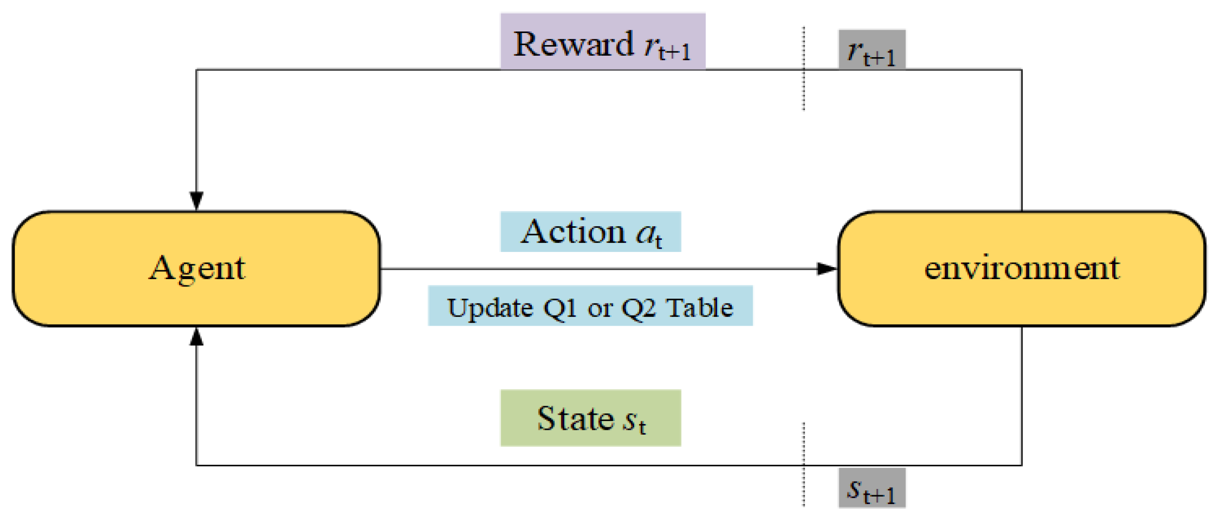
Figure 2.
DQDCS flowchart.
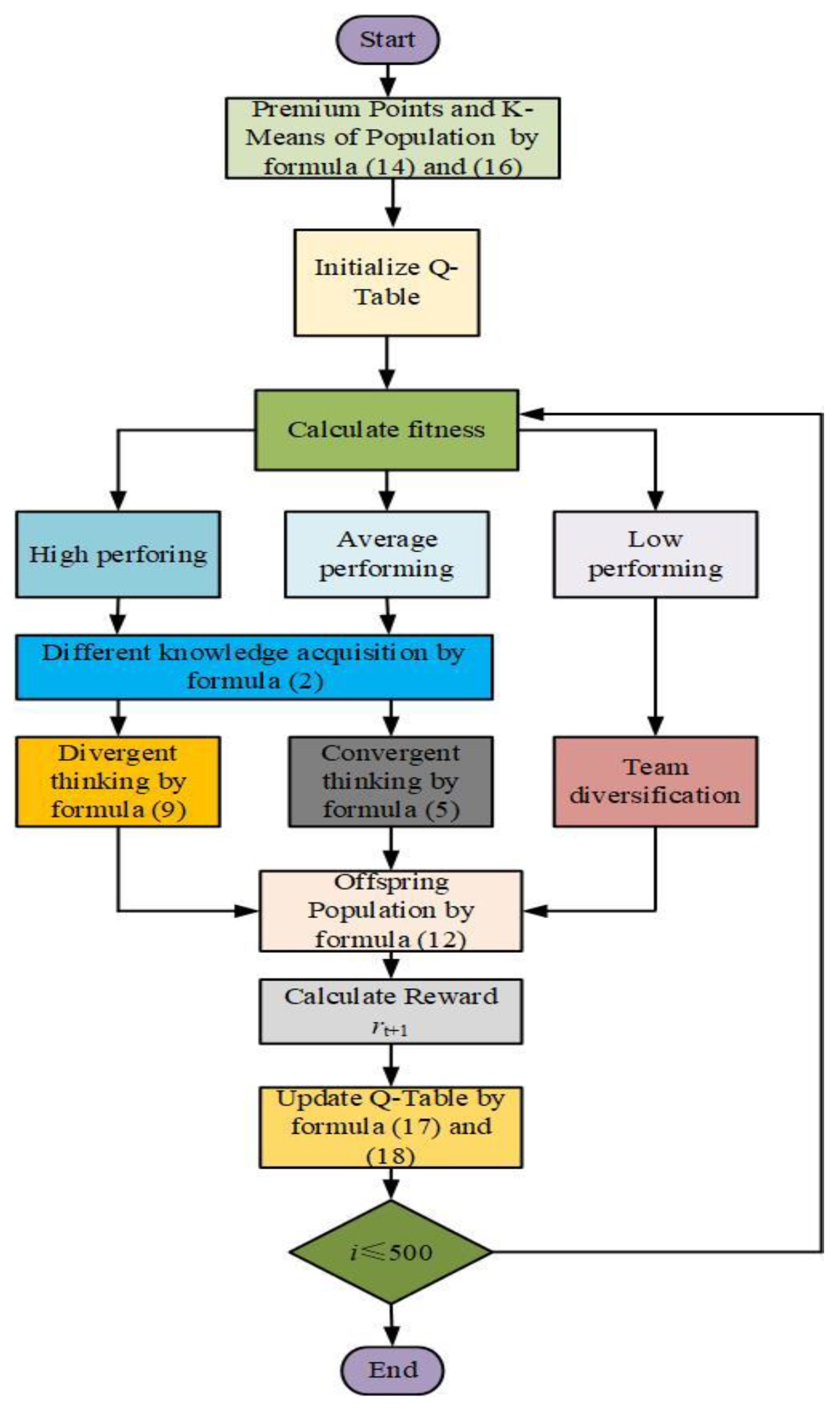
Figure 3.
Convergence curve of CEC2019 benchmark tests.
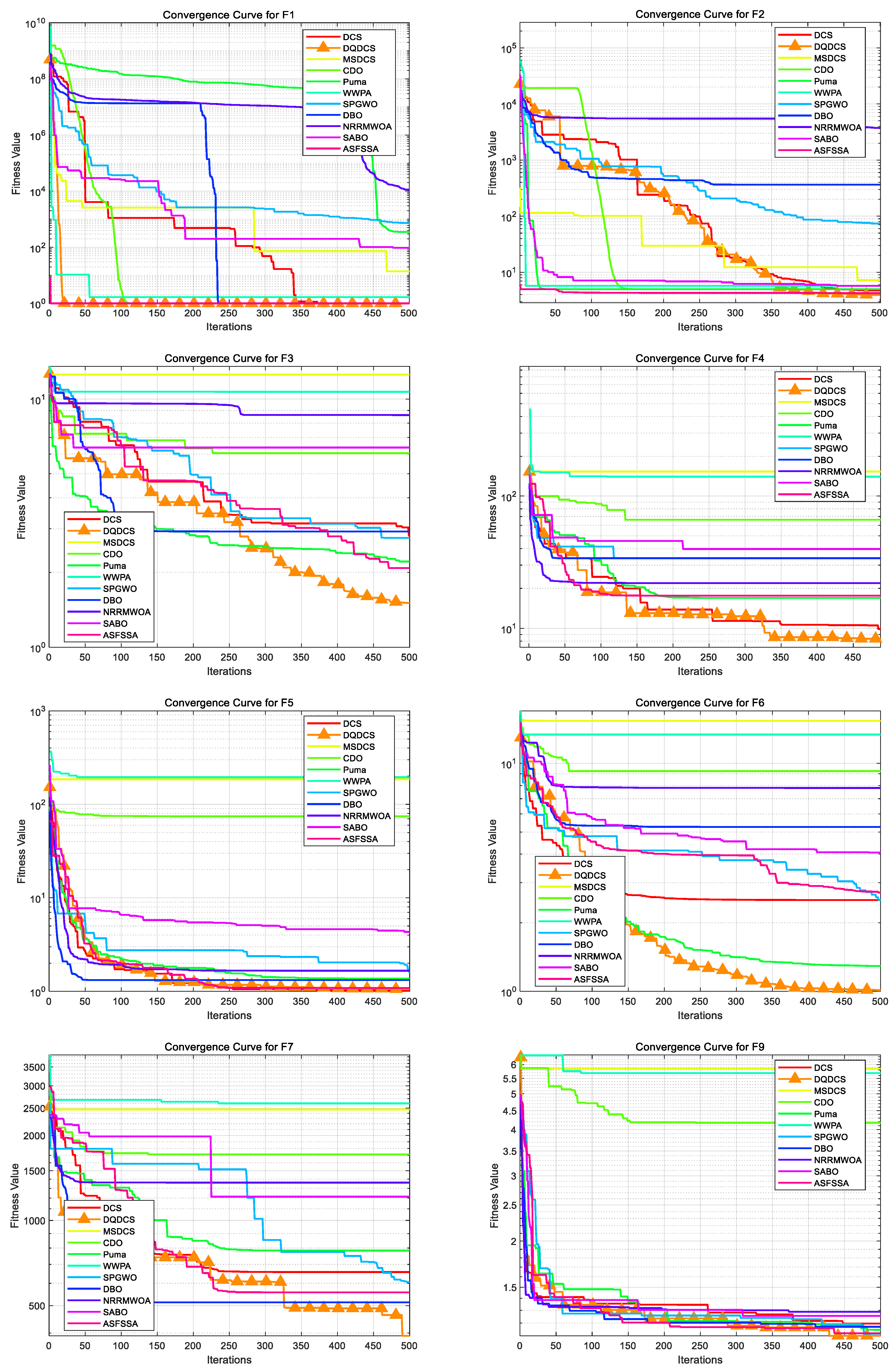
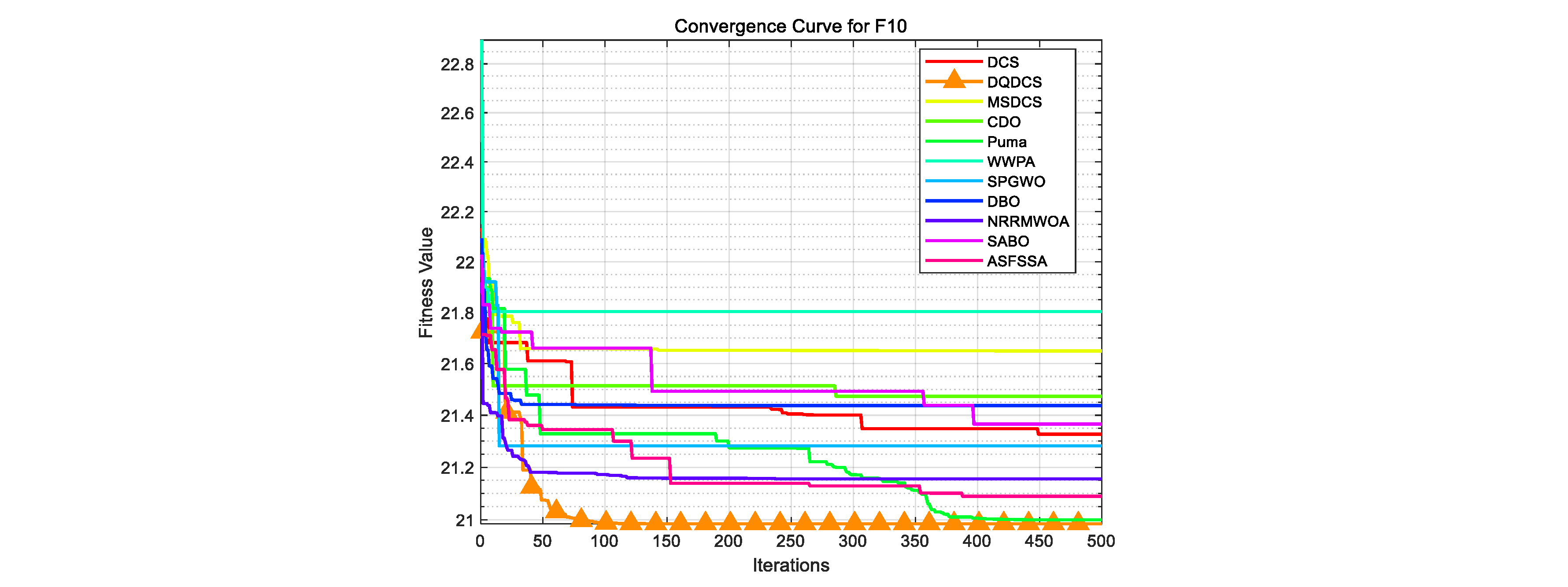
Figure 4.
Boxplots of CEC2019 benchmark functions.
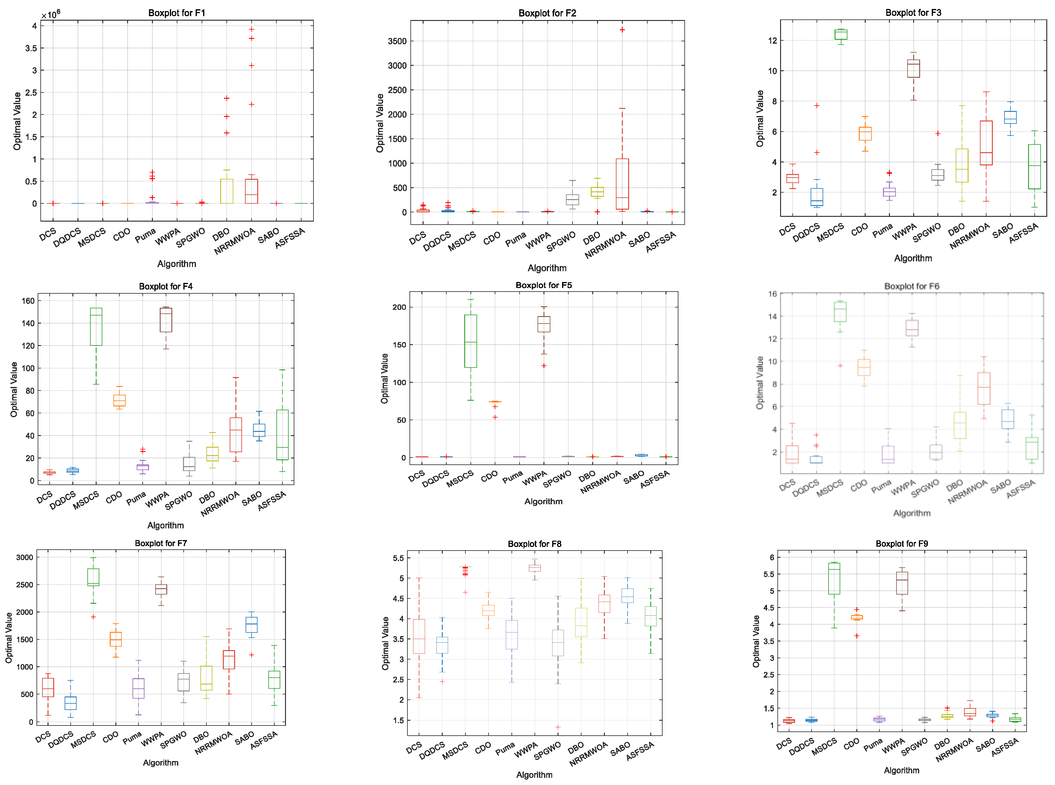

Figure 5.
Convergence curve of CEC2022 benchmark tests.
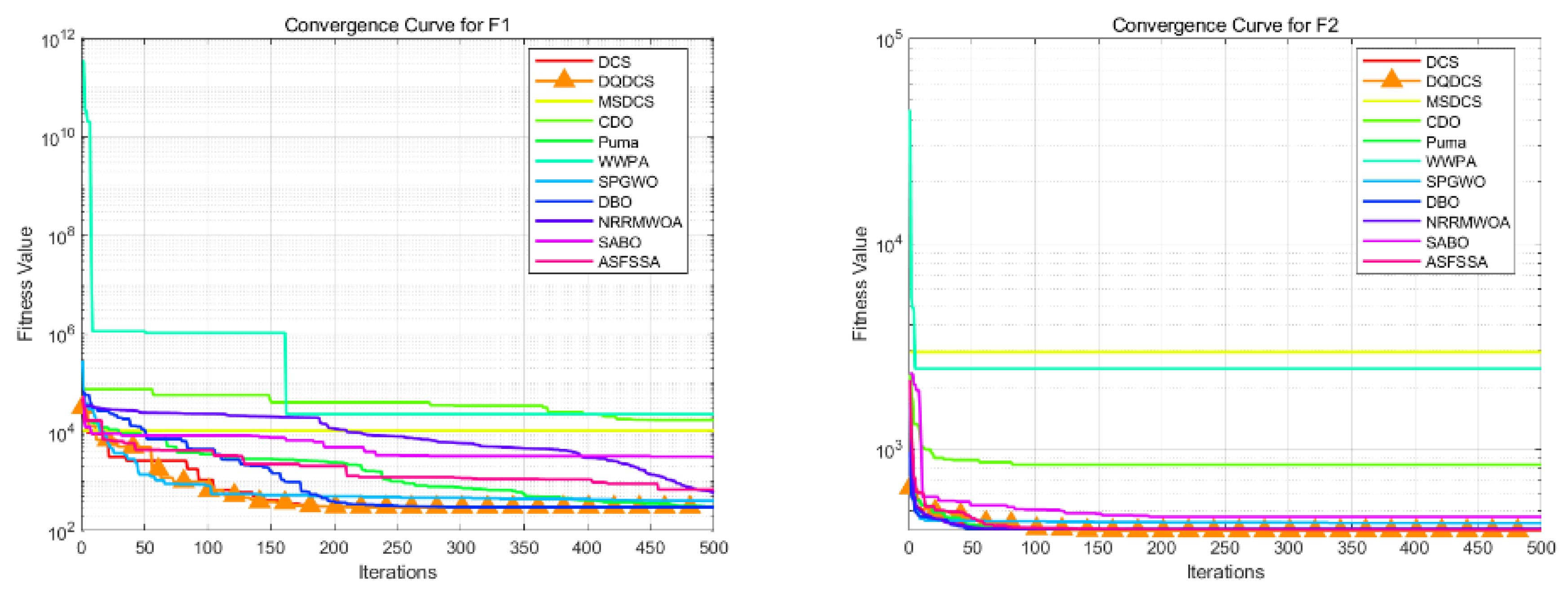
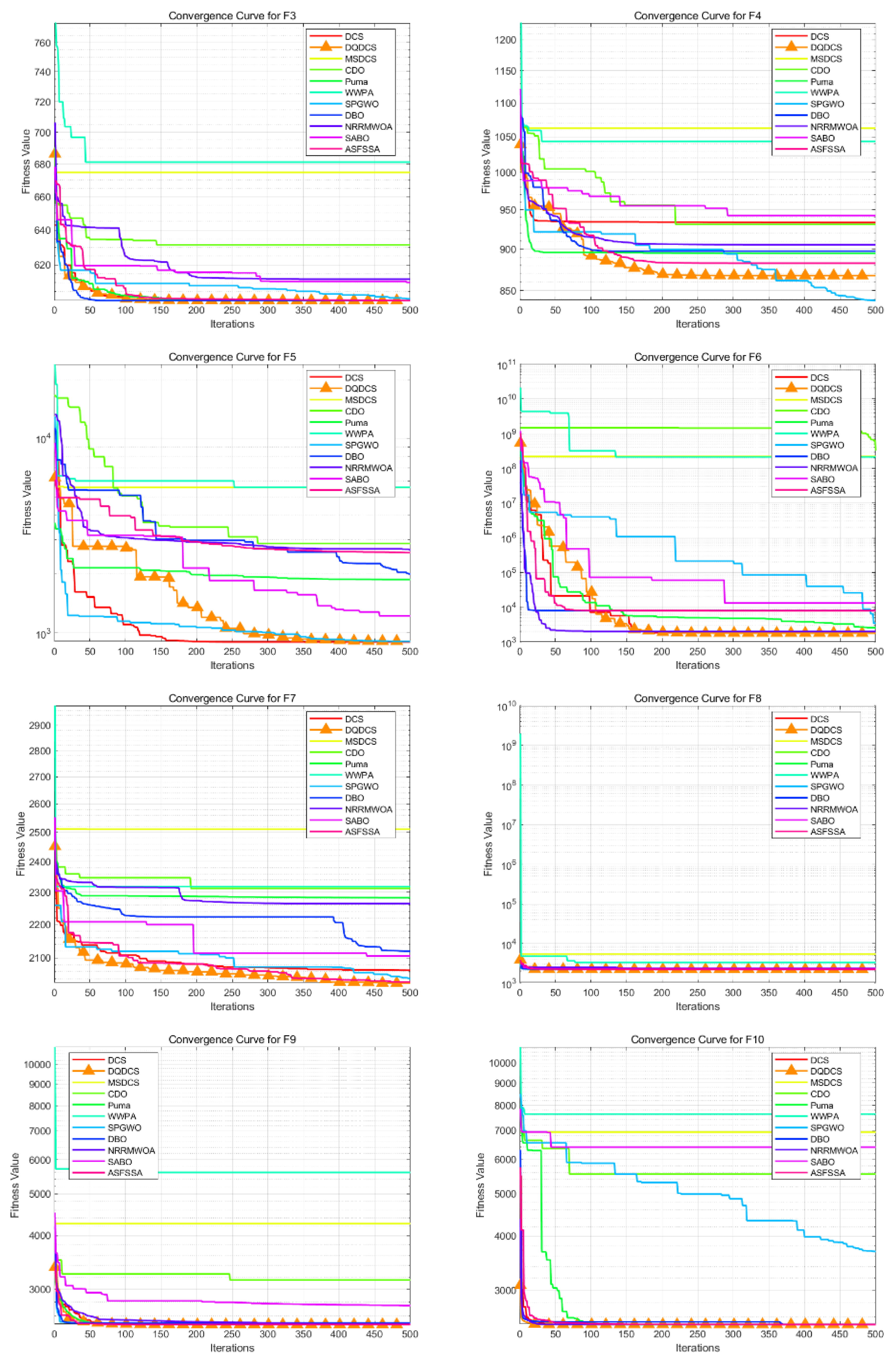
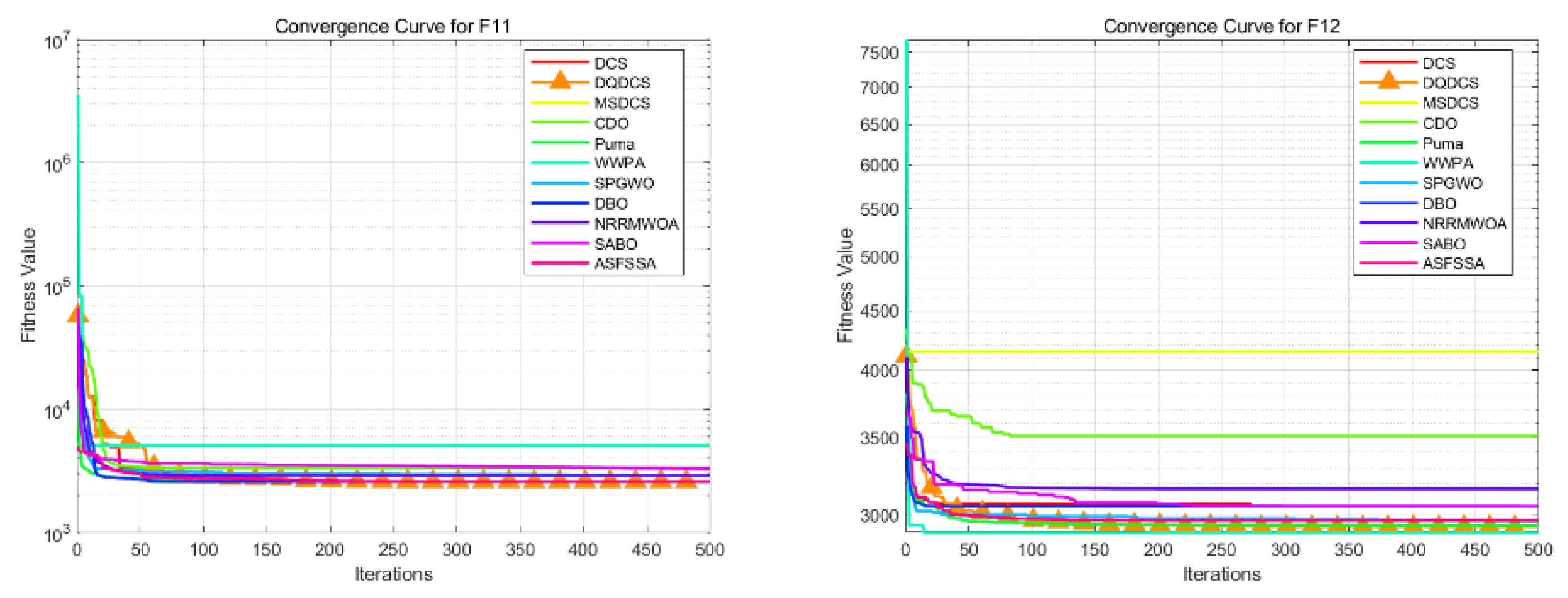
Figure 6.
Boxplots of CEC2022 benchmark functions.
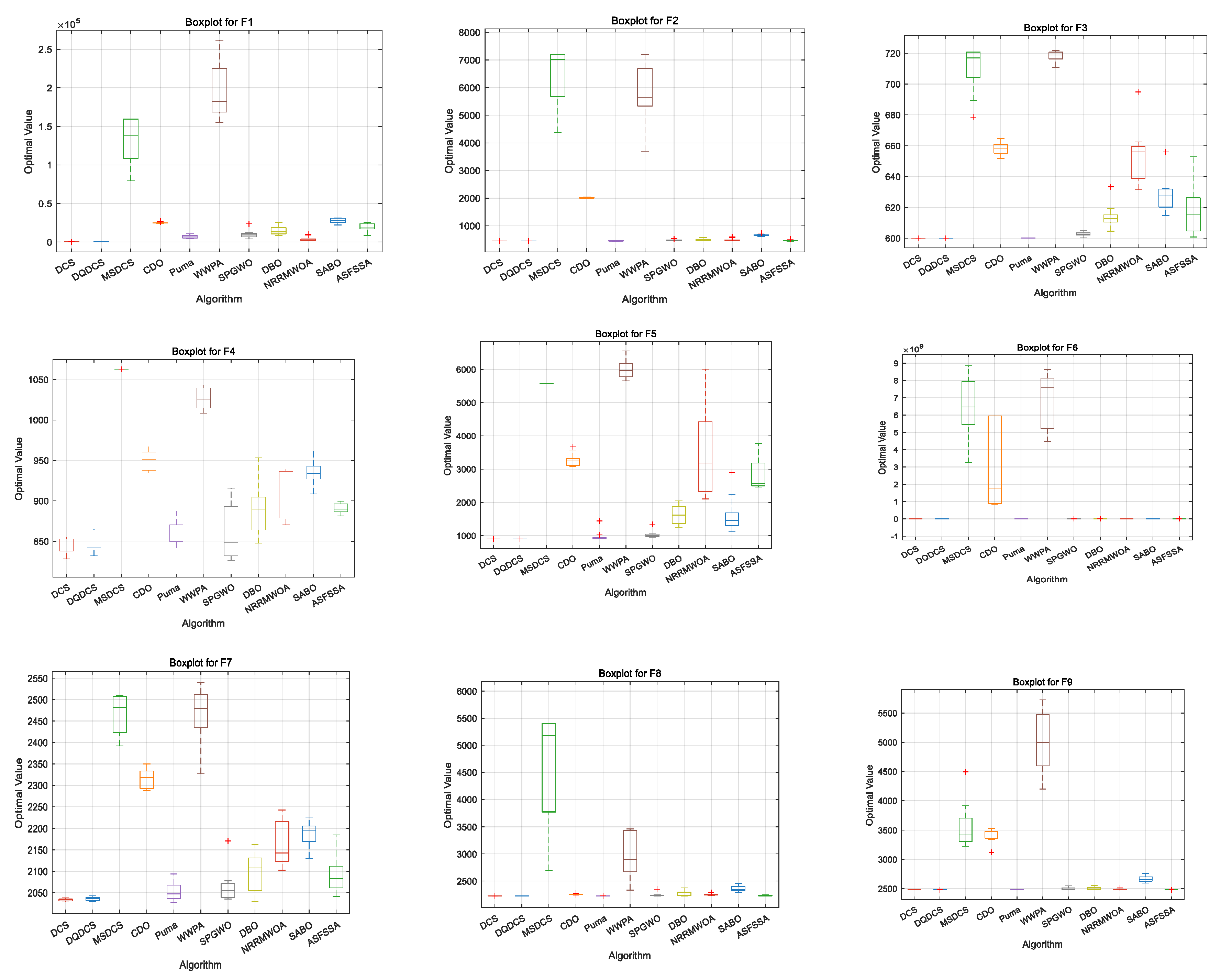
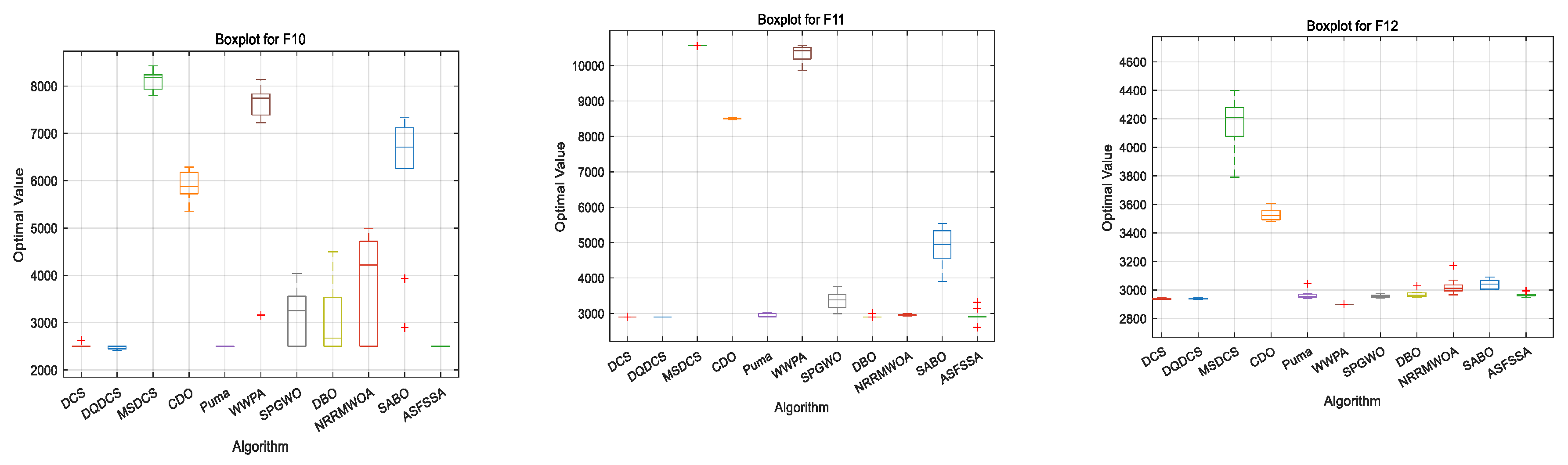
Figure 7.
Static pressure thrust bearing.
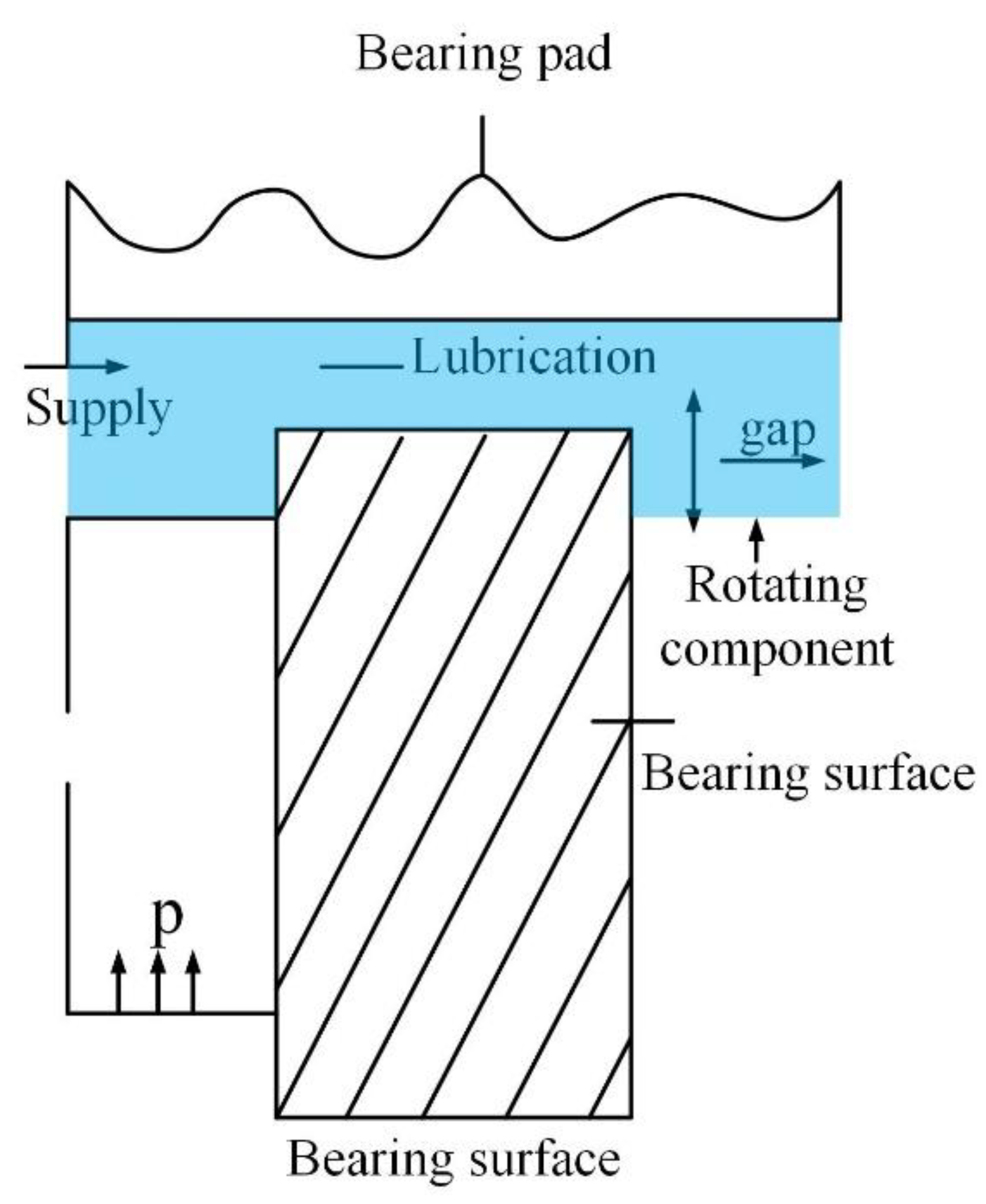
Figure 8.
SOPWM for 3-level inverters.
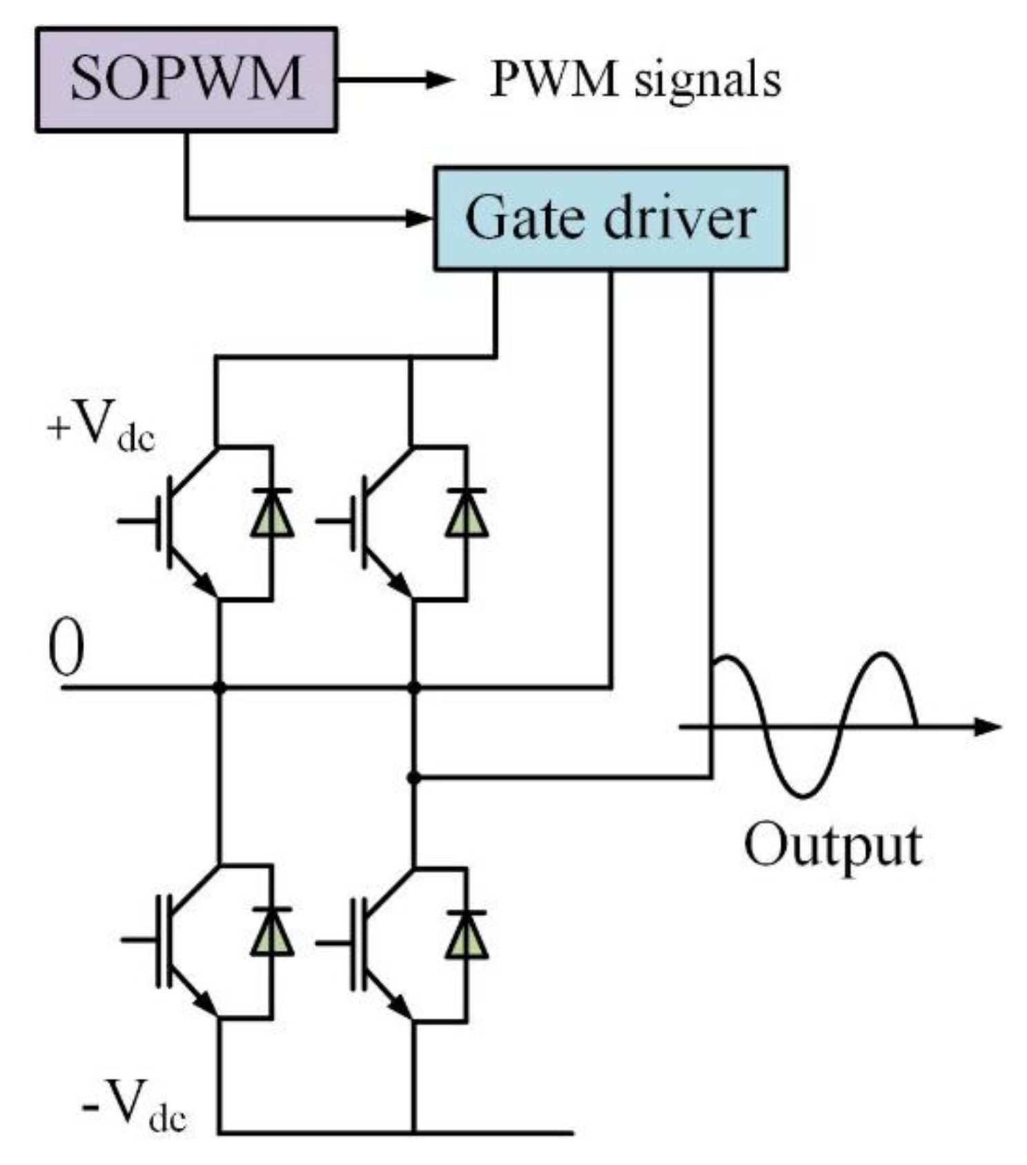
Figure 9.
Comparison charts of CPU running times of various algorithms for static pressure thrust bearing.
Figure 9.
Comparison charts of CPU running times of various algorithms for static pressure thrust bearing.
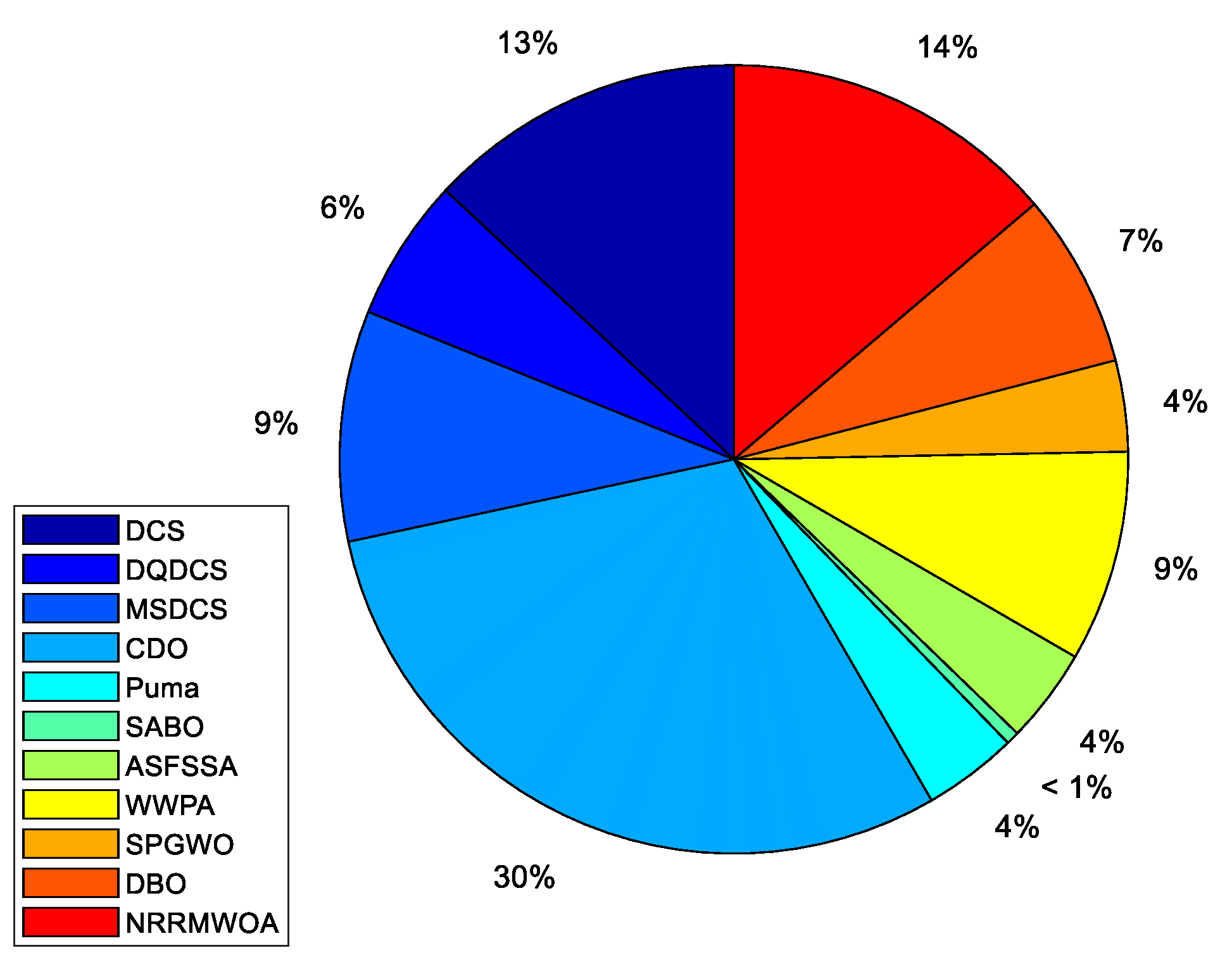
Figure 10.
Comparison charts of CPU running times of various algorithms for SOPWM for 3-level inverters.
Figure 10.
Comparison charts of CPU running times of various algorithms for SOPWM for 3-level inverters.
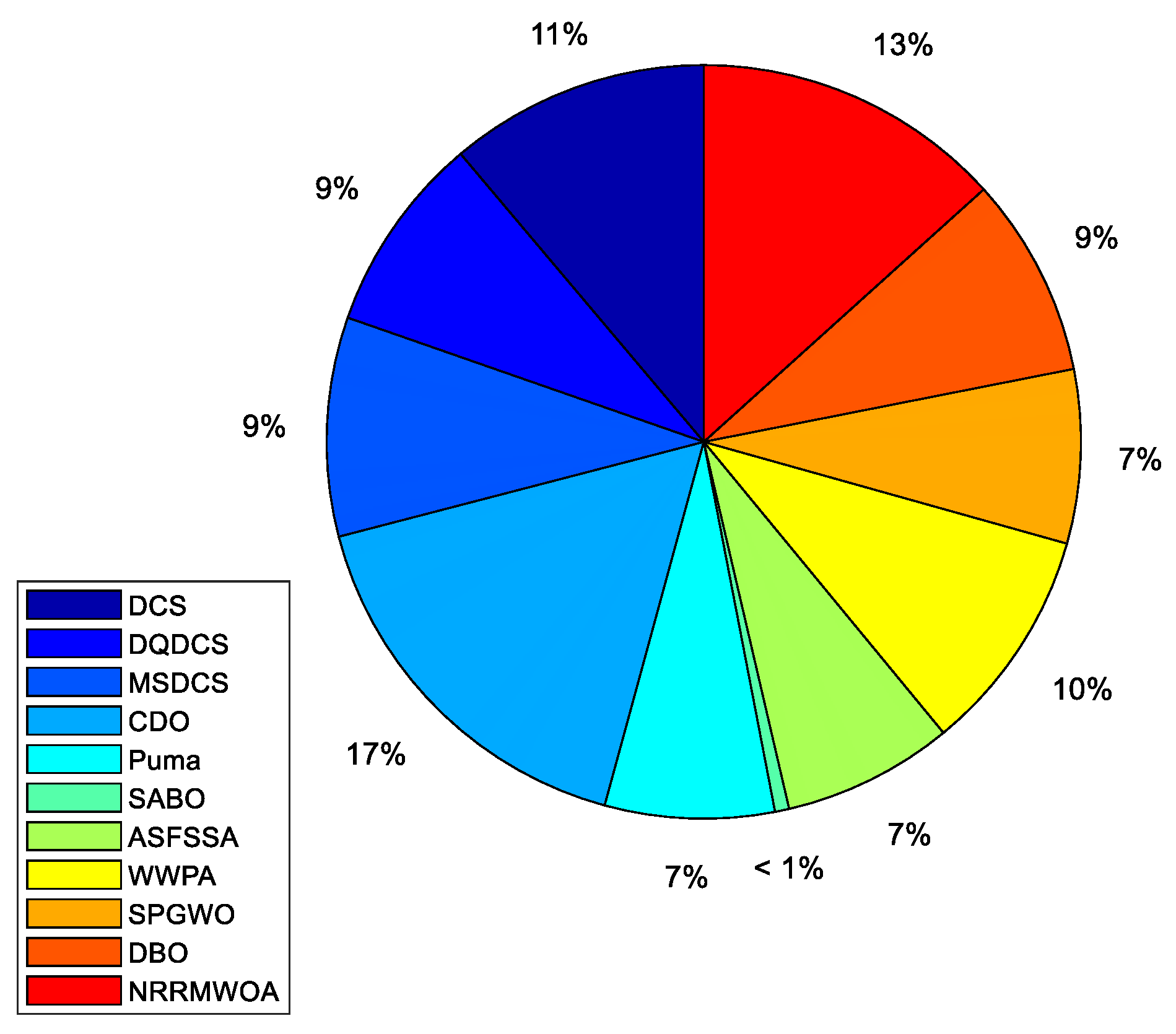
Table 3.
Testing results of CEC2022 benchmark functions.
| Function | Algorithm | Best | Mean | Std |
|---|---|---|---|---|
| F1 | DCS | 300 | 301 | 3.8519e-13 |
| DQDCS | 300 | 300 | 6.8317e-14 | |
| MSDCS | 10766.7503 | 10766.7571 | 0.013964 | |
| CDO | 7490.1964 | 20512.7673 | 13607.6136 | |
| Puma | 300.0023 | 301.2711 | 2.5835 | |
| WWPA | 8455.8816 | 236150.7116 | 1491237.9285 | |
| SPGWO | 304.8303 | 797.5061 | 1028.1107 | |
| DBO | 300 | 361.9946 | 341.4715 | |
| NRRMWOA | 358.8157 | 3032.3131 | 2230.1134 | |
| SABO | 1195.7814 | 3379.0063 | 1311.4349 | |
| ASFSSA | 309.4622 | 586.0842 | 281.7238 | |
| F2 | DCS | 400 | 405.5275 | 3.4253 |
| DQDCS | 400.0035 | 403.425 | 3.6114 | |
| MSDCS | 750.1737 | 2491.5488 | 960.6972 | |
| CDO | 570.9415 | 835.2859 | 49.4592 | |
| Puma | 400 | 406.3943 | 7.2844 | |
| WWPA | 972.5671 | 3270.4214 | 1414.9336 | |
| SPGWO | 400.5352 | 415.7896 | 14.3696 | |
| DBO | 400.0218 | 424.2427 | 29.16 | |
| NRRMWOA | 400.0781 | 422.0518 | 27.9517 | |
| SABO | 404.4744 | 448.4682 | 21.9722 | |
| ASFSSA | 400.0102 | 413.4404 | 19.3205 | |
| F3 | DCS | 600 | 600 | 3.5703e-07 |
| DQDCS | 600.0001 | 600.0005 | 3.2297e-07 | |
| MSDCS | 643.6113 | 682.7551 | 10.18 | |
| CDO | 627.5045 | 634.8725 | 3.539 | |
| Puma | 600 | 600 | 0.00026748 | |
| WWPA | 662.8221 | 687.3778 | 7.5308 | |
| SPGWO | 600.0541 | 600.4967 | 0.68095 | |
| DBO | 600 | 601.7739 | 2.6285 | |
| NRRMWOA | 601.6986 | 621.4008 | 11.8169 | |
| SABO | 603.078 | 612.0294 | 7.4192 | |
| ASFSSA | 600 | 602.2958 | 6.5591 | |
| F4 | DCS | 803.5611 | 809.1824 | 2.9573 |
| DQDCS | 801.7438 | 809.0859 | 1.0729 | |
| MSDCS | 867.3885 | 896.995 | 4.0671 | |
| CDO | 828.5143 | 845.4771 | 6.2154 | |
| Puma | 806.9647 | 818.357 | 6.8807 | |
| WWPA | 864.4186 | 887.3275 | 8.2043 | |
| SPGWO | 800.3831 | 800.9999 | 6.6974 | |
| DBO | 807.9597 | 829.8866 | 10.517 | |
| NRRMWOA | 809.95 | 835.8238 | 14.4457 | |
| SABO | 819.7184 | 838.0276 | 8.1862 | |
| ASFSSA | 811.9395 | 829.6198 | 5.4414 | |
| F5 | DCS | 900 | 900 | 2.2852e-14 |
| DQDCS | 900 | 900 | 2.0549e-14 | |
| MSDCS | 2066.3081 | 2246.8891 | 21.1599 | |
| CDO | 1248.3716 | 1377.5434 | 69.9206 | |
| Puma | 900 | 900.3861 | 0.57066 | |
| WWPA | 1860.8209 | 2380.0621 | 185.2868 | |
| SPGWO | 900 | 900.0042 | 10.5999 | |
| DBO | 900 | 916.4121 | 57.1606 | |
| NRRMWOA | 906.326 | 1253.0823 | 278.8837 | |
| SABO | 901.1913 | 925.9241 | 16.9796 | |
| ASFSSA | 901.7282 | 1398.8497 | 174.1701 | |
| F6 | DCS | 1800.0368 | 1805.6947 | 1.5327 |
| DQDCS | 1800.0238 | 1801.939 | 2.0455 | |
| MSDCS | 70252227.0095 | 207374163.4593 | 33963697.1425 | |
| CDO | 15167928.0263 | 157093751.8526 | 240080753.4813 | |
| Puma | 1807.9235 | 2063.024 | 734.8686 | |
| WWPA | 8608986.8261 | 185293465.0815 | 73329210.9276 | |
| SPGWO | 1960.6464 | 5799.1861 | 2292.3454 | |
| DBO | 1895.1412 | 4731.5419 | 2375.8384 | |
| NRRMWOA | 1846.6869 | 3977.1499 | 2076.5281 | |
| SABO | 2459.4489 | 20110.6228 | 11920.7947 | |
| ASFSSA | 1930.1248 | 5432.4366 | 1903.6817 | |
| F7 | DCS | 2027.974 | 2049.2777 | 14.7551 |
| DQDCS | 2000.229 | 2001.6385 | 2.837 | |
| MSDCS | 2337.8697 | 2447.3738 | 69.1571 | |
| CDO | 2231.4056 | 2300.052 | 30.0378 | |
| Puma | 2151.4621 | 2192.5272 | 43.688 | |
| WWPA | 2306.8139 | 2451.1073 | 90.2488 | |
| SPGWO | 2034.3498 | 2057.4032 | 25.2011 | |
| DBO | 2032.3433 | 2090.2749 | 34.7803 | |
| NRRMWOA | 2101.6025 | 2198.9024 | 60.3948 | |
| SABO | 2105.6682 | 2178.9918 | 37.0986 | |
| ASFSSA | 2030.9544 | 2094.5985 | 29.2648 | |
| F8 | DCS | 2222.0212 | 2225.7348 | 5.0729 |
| DQDCS | 2200.7186 | 2208.8764 | 7.0158 | |
| MSDCS | 2846.8452 | 3952.5994 | 1101.3132 | |
| CDO | 2243.644 | 2251.946 | 6.6606 | |
| Puma | 2226.3281 | 2353.5188 | 125.6302 | |
| WWPA | 2551.5422 | 2917.5036 | 244.8562 | |
| SPGWO | 2224.4404 | 2229.9677 | 4.8594 | |
| DBO | 2233.7582 | 2301.6076 | 63.7515 | |
| NRRMWOA | 2237.5665 | 2262.526 | 34.2888 | |
| SABO | 2278.1633 | 2356.1119 | 64.2682 | |
| ASFSSA | 2222.1835 | 2227.1796 | 4.6573 | |
| F9 | DCS | 2529.2844 | 2529.2844 | 0 |
| DQDCS | 2480.7821 | 2480.2942 | 0.027562 | |
| MSDCS | 3371.8015 | 3996.9709 | 412.0453 | |
| CDO | 3151.4652 | 3426.8386 | 126.0153 | |
| Puma | 2480.7976 | 2480.8202 | 0.017425 | |
| WWPA | 3370.7773 | 4492.3652 | 979.6033 | |
| SPGWO | 2481.1805 | 2500.7716 | 22.002 | |
| DBO | 2480.9125 | 2496.6431 | 20.4099 | |
| NRRMWOA | 2481.1486 | 2491.6469 | 14.7268 | |
| SABO | 2603.3814 | 2699.6239 | 46.6498 | |
| ASFSSA | 2480.7813 | 2480.8064 | 0.067892 | |
| F10 | DCS | 2500.3438 | 2515.1856 | 46.6588 |
| DQDCS | 2500.1542 | 2503.504 | 18.4699 | |
| MSDCS | 6937.0014 | 7963.4014 | 476.9702 | |
| CDO | 4832.6414 | 5873.0597 | 506.4387 | |
| Puma | 2500.638 | 2515.0468 | 45.15 | |
| WWPA | 7228.1772 | 7552.068 | 210.5838 | |
| SPGWO | 2500.5073 | 3312.8457 | 742.2508 | |
| DBO | 2500.8157 | 2930.6677 | 678.0253 | |
| NRRMWOA | 2501.3194 | 4062.9987 | 1135.7437 | |
| SABO | 2858.03 | 5556.1544 | 1635.5186 | |
| ASFSSA | 2500.7384 | 2630.7374 | 410.1658 | |
| F11 | DCS | 2600 | 2646.5043 | 108.0761 |
| DQDCS | 2600 | 2639 | 103.2576 | |
| MSDCS | 5105.1466 | 5105.1769 | 0.082861 | |
| CDO | 3329.1224 | 3343.2781 | 5.6324 | |
| Puma | 2600.0001 | 2637.3103 | 118.4636 | |
| WWPA | 3712.7414 | 4917.2808 | 262.7002 | |
| SPGWO | 2601.1884 | 2904.431 | 130.4169 | |
| DBO | 2600 | 2814.9987 | 171.69 | |
| NRRMWOA | 2600.698 | 2901.0184 | 130.9309 | |
| SABO | 2832.4972 | 3233.2798 | 104.4736 | |
| ASFSSA | 2600 | 2663.175 | 113.4852 | |
| F12 | DCS | 2988.2699 | 3219.0423 | 181.9443 |
| DQDCS | 2700.6186 | 2722.0363 | 2.1318 | |
| MSDCS | 3624.3346 | 4070.0287 | 301.5474 | |
| CDO | 3478.4691 | 3508.6705 | 25.8794 | |
| Puma | 2939.2542 | 2951.6242 | 13.3077 | |
| WWPA | 2900.0048 | 2900.005 | 5.3612e-05 | |
| SPGWO | 2937.2174 | 2955.9256 | 13.3377 | |
| DBO | 2939.8499 | 2973.7347 | 40.5269 | |
| NRRMWOA | 2958.0579 | 3044.9336 | 70.3033 | |
| SABO | 2994.7804 | 3054.3338 | 38.4792 | |
| ASFSSA | 2945.5917 | 2962.4681 | 13.8506 |
Table 4.
Wilcoxon rank-sum test results for CEC2022 benchmark functions.
| DQDCS vs. | DCS | MSDCS | CDO | Puma | WWPA | SPGWO | DBO | NRRMWOA | SABO | ASFSSA |
| F1 | 4.40E-04 | 1.83E-04 | 1.83E-04 | 1.83E-04 | 1.83E-04 | 7.69E-04 | 1.83E-04 | 4.40E-04 | 1.83E-04 | 1.83E-04 |
| F2 | 3.61E-03 | 1.83E-04 | 1.83E-04 | 1.83E-04 | 1.83E-04 | 1.83E-04 | 8.90E-03 | 1.83E-04 | 1.83E-04 | 1.83E-04 |
| F3 | 2.83E-03 | 1.83E-04 | 1.83E-04 | 1.83E-04 | 1.83E-04 | 2.20E-03 | 1.83E-04 | 1.83E-04 | 1.83E-04 | 1.83E-04 |
| F4 | 9.11E-03 | 1.83E-04 | 1.83E-04 | 4.52E-02 | 1.83E-04 | 1.13E-02 | 2.20E-03 | 8.90E-03 | 1.83E-04 | 5.21E-03 |
| F5 | 2.57E-02 | 1.83E-04 | 1.83E-04 | 1.83E-04 | 1.83E-04 | 1.01E-03 | 1.83E-04 | 1.83E-04 | 1.83E-04 | 1.83E-04 |
| F6 | 6.23E-02 | 1.83E-04 | 1.83E-04 | 1.83E-04 | 1.83E-04 | 1.73E-02 | 1.40E-02 | 2.20E-03 | 1.83E-04 | 4.40E-04 |
| F7 | 3.12E-02 | 1.83E-04 | 1.83E-04 | 1.83E-04 | 1.83E-04 | 3.34E-02 | 2.83E-03 | 1.83E-04 | 1.83E-04 | 6.40E-02 |
| F8 | 3.12E-02 | 1.83E-04 | 1.83E-04 | 4.40E-04 | 1.83E-04 | 2.20E-03 | 1.04E-02 | 1.83E-04 | 1.83E-04 | 4.40E-04 |
| F9 | 1.83E-04 | 1.83E-04 | 1.83E-04 | 1.83E-04 | 1.83E-04 | 1.83E-04 | 2.80E-03 | 1.83E-04 | 1.83E-04 | 1.83E-04 |
| F10 | 1.71E-02 | 1.83E-04 | 1.83E-04 | 2.21E-03 | 1.83E-04 | 1.73E-02 | 9.11E-03 | 1.83E-04 | 1.83E-04 | 3.09E-02 |
| F11 | 4.52E-02 | 1.83E-04 | 1.83E-04 | 1.83E-04 | 1.83E-04 | 1.40E-02 | 2.20E-03 | 1.83E-04 | 1.83E-04 | 1.83E-04 |
| F12 | 1.73E-02 | 1.83E-04 | 1.83E-04 | 1.01E-03 | 1.83E-04 | 7.69E-04 | 1.01E-03 | 2.46E-04 | 1.83E-04 | 2.46E-04 |
Table 5.
Optimization results of static pressure thrust bearing.
| name | x1 | x2 | x3 | x4 | worst | best | std | mean | median |
| DCS | 1.59727828E-05 | 1.00023775E+00 | 1.47915355E+01 | 1.59942442E+01 | 1.06923430E+09 | 1.07206086E+09 | 6.61825327E+05 | 1.07014876E+09 | 1.06997430E+09 |
| DQDCS | 1.60000000E-05 | 1.00000000E+00 | 1.48001689E+01 | 1.60000000E+01 | 1.06894753E+09 | 1.06954809E+09 | 1.34312464E+05 | 1.06898081E+09 | 1.06894753E+09 |
| MSDCS | 1.17291046E-05 | 1.79130942E+00 | 5.70274004E+00 | 1.59413101E+01 | 1.40136705E+09 | 5.22419187E+14 | 1.19485993E+14 | 3.57212782E+13 | 1.17985612E+11 |
| Puma | 1.60000000E-05 | 1.00000000E+00 | 1.48003474E+01 | 1.60000000E+01 | 1.06896145E+09 | 1.12825463E+09 | 1.37399596E+07 | 1.07613384E+09 | 1.07044585E+09 |
| CDO | 1.60000000E-05 | 1.00000000E+00 | 1.48163617E+01 | 1.60000000E+01 | 1.07047191E+09 | 1.15997503E+09 | 2.15231379E+07 | 1.09774625E+09 | 1.09665275E+09 |
| WWPA | 4.73396390E-01 | 1.60123665E+06 | 3.94298347E+05 | 3.91671659E+05 | -2.22716152E+11 | 2.35796666E+10 | 5.37550187E+10 | 1.52405939E+10 | 1.15527859E+09 |
| SPGWO | 1.60000000E-05 | 1.00000000E+00 | 1.48012444E+01 | 1.60000000E+01 | 1.06904448E+09 | 1.32319148E+09 | 5.65555937E+07 | 1.08297369E+09 | 1.07012621E+09 |
| DBO | 1.60000000E-05 | 1.00000000E+00 | 1.48001689E+01 | 1.60000000E+01 | 1.06894753E+09 | 1.47869424E+09 | 9.15951602E+07 | 1.08955220E+09 | 1.06894753E+09 |
| NRRMWOA | 1.60000000E-05 | 1.00000000E+00 | 1.48001572E+01 | 1.60000000E+01 | 1.06894764E+09 | 1.10966892E+09 | 1.11408274E+07 | 1.07630514E+09 | 1.07166285E+09 |
| SABO | 1.60000000E-05 | 1.00000000E+00 | 1.48145609E+01 | 1.60000000E+01 | 1.07029905E+09 | 1.49353781E+09 | 1.44018113E+08 | 1.18985405E+09 | 1.12582885E+09 |
| ASFSSA | 1.60000000E-05 | 1.00000000E+00 | 1.48002442E+01 | 1.60000000E+01 | 1.06895191E+09 | 1.07108086E+09 | 6.86835160E+05 | 1.06948901E+09 | 1.06929758E+09 |
Table 6.
Optimization results of SOPWM for 3-level inverters.
| name | x1 | x2 | x3 | x4 | worst | best | std | mean | median |
| DCS | 5.56990820E-01 | 1.55691929E+00 | 1.55632264E+00 | 1.57069023E+00 | 9.95709896E-01 | 1.00272898E+00 | 1.67135890E-03 | 9.98300957E-01 | 9.98148422E-01 |
| DQDCS | 5.56423139E-01 | 1.57079633E+00 | 1.57037521E+00 | 1.57079633E+00 | 9.95405132E-01 | 9.95440460E-01 | 7.97475504E-06 | 9.95408550E-01 | 9.95405849E-01 |
| MSDCS | 3.98818649E-01 | 1.41758251E+00 | 1.49139957E+00 | 1.54923355E+00 | 1.61761236E+00 | 1.05741270E+02 | 3.01338199E+01 | 2.76842562E+01 | 1.86908292E+01 |
| Puma | 5.56414603E-01 | 1.57079633E+00 | 1.57037818E+00 | 1.57079633E+00 | 9.95405129E-01 | 9.95580896E-01 | 5.19507407E-05 | 9.95430761E-01 | 9.95406675E-01 |
| CDO | 5.55834510E-01 | 1.57079633E+00 | 1.57079633E+00 | 1.57079633E+00 | 9.95593045E-01 | 1.14082188E+00 | 6.15210384E-02 | 1.05110186E+00 | 1.00665276E+00 |
| WWPA | 2.85068113E+03 | 1.48395345E+04 | 1.57150650E+04 | 7.21160329E+04 | 1.48895835E+00 | 7.80431264E+01 | 1.82177239E+01 | 1.19310968E+01 | 4.09729542E+00 |
| SPGWO | 5.56714311E-01 | 1.57079633E+00 | 1.57027734E+00 | 1.57079633E+00 | 9.95418349E-01 | 1.16755946E+00 | 6.26457711E-02 | 1.02849798E+00 | 9.95582535E-01 |
| DBO | 5.56418317E-01 | 1.57079633E+00 | 1.57037750E+00 | 1.57079633E+00 | 9.95405127E-01 | 1.16755679E+00 | 3.97313485E-02 | 1.00687810E+00 | 9.95580896E-01 |
| NRRMWOA | 5.56416113E-01 | 1.57079633E+00 | 1.57037874E+00 | 1.57079633E+00 | 9.95405128E-01 | 1.16755772E+00 | 5.29815832E-02 | 1.01263761E+00 | 9.95405148E-01 |
| SABO | 5.55660648E-01 | 1.57079633E+00 | 1.57079633E+00 | 1.57079633E+00 | 9.95581236E-01 | 9.96458735E-01 | 2.43692395E-04 | 9.95726761E-01 | 9.95624926E-01 |
| ASFSSA | 5.56418323E-01 | 1.57079633E+00 | 1.57037750E+00 | 1.57079633E+00 | 9.95405127E-01 | 1.20665475E+00 | 7.59187361E-02 | 1.04151473E+00 | 9.95508388E-01 |
Disclaimer/Publisher’s Note: The statements, opinions and data contained in all publications are solely those of the individual author(s) and contributor(s) and not of MDPI and/or the editor(s). MDPI and/or the editor(s) disclaim responsibility for any injury to people or property resulting from any ideas, methods, instructions or products referred to in the content. |
© 2025 by the authors. Licensee MDPI, Basel, Switzerland. This article is an open access article distributed under the terms and conditions of the Creative Commons Attribution (CC BY) license (http://creativecommons.org/licenses/by/4.0/).
Copyright: This open access article is published under a Creative Commons CC BY 4.0 license, which permit the free download, distribution, and reuse, provided that the author and preprint are cited in any reuse.


