
Submitted:
02 April 2025
Posted:
03 April 2025
You are already at the latest version
Abstract
Characterization of soil attribute variability often requires dense sampling grids, which can be economically unfeasible. A possible solution is to perform targeted sampling based on previously collected data. The objective of this research was to develop a method for mapping soil attributes based on Management Zones (MZs) delineated from Sentinel-1 radar data. Sentinel-1 images were used to create time profiles of six indices based on VV (vertical-vertical) and VH (vertical-horizontal) backscatter in two agricultural fields. MZs were delineated by analyzing indices and VV/VH backscatter bands individually through two approaches: (1) fuzzy k-means clustering directly applied to the indices' time series, and (2) dimensionality reduction using deep-learning autoencoders followed by fuzzy k-means clustering. The best combination of index and MZs delineation approach was compared with four soil attribute mapping methods: conventional (single composite sample), high-density uniform grid (one sample per hectare), rectangular cells (one composite sample per cell of 5 to 10 hectares), and random cells (one composite sample per cell of varying sizes). Leave-one-out cross-validation evaluated the performance of each sampling method. Results showed that combining VV/VH index and autoencoders for MZs delineation provided more accurate soil attribute estimates, outperforming the conventional, random cells, and often the rectangular cell method.
Keywords:
Precision agriculture
; Remote sensing
; Soil sampling
1. Introduction
Information regarding the spatial and temporal variability of soil attributes plays a crucial role in the development of effective soil management strategies. By examining these data, farmers can adopt the most suitable cultivars and plant population densities for each specific point within the production area. This, in turn, facilitates the precise determination of the required amounts of fertilizers and soil acidity correctives, not only to maximize financial returns but also to promote more sustainable production [1].
However, developing an effective strategy for collecting data to characterize the spatial and temporal variability of soil attributes is a complex and challenging task. Research has highlighted the importance of establishing dense sampling grids, with a minimum density of one sample per hectare, to adequately capture the variability of soil attributes [2,3,4]. [5] demonstrated that variograms used to infer soil attributes at unsampled points are unreliable when based on fewer than 100 data points, potentially leading to inaccurate estimates with significant margins of error. Therefore, grid sampling can provide a precise basis for variable rate application, but the costs and labour requirements, especially in extensive areas with high variability, suggest that other approaches may be more economical [6].
To understand the spatial and temporal variability of soil attributes without the need to establish dense sampling grids, studies have demonstrated the potential of using soil sensors or the crop itself as a 'soil sensor' [1]. Apparent soil electrical conductivity sensors, yield maps, and canopy reflectance indices can provide maps with different spatial and temporal variability patterns and be used to delineate homogeneous areas known as Management Zones (MZs) [7,8,9,10,11,12]. Within each MZs, low variability of soil attributes is assumed, recommending the collection of a single composite sample. Based on specific levels of these attributes, targeted management practices for each MZs are established. This strategy reduces soil sampling costs compared to dense sampling grids, while simultaneously providing a better distribution of management practices (cultivars, plant density, fertilizers) compared to the conventional soil sampling method, in which only a single attribute level and consequently a single management strategy is determined for the entire area.
Although the development of MZs through these methods represents an advancement in precision agriculture, their adoption among farmers remains limited. This limitation is largely due to difficulties in accessing reliable historical yield maps, electrical conductivity data, and multispectral satellite image time series with high temporal resolution. For example, yield maps have been available since the early 1990s, yet their adoption is still limited to only 5% to 25% of the total cultivated area in the United States for crops such as winter wheat, cotton, sorghum, and rice, and 45% for corn and soybean crops [13]. Apparent soil electrical conductivity presents itself as an attractive alternative because it can be quickly and easily measured for fields using electromagnetic induction instruments. However, this type of data collection strongly depends on specialized service providers for data acquisition and interpretation, whose availability varies across agricultural regions, complicating the implementation of this technology.
The use of multispectral optical images, freely available from orbital platforms such as Landsat-8 and Sentinel-2, enables remote service delivery and extensive spatial coverage. However, its application faces significant challenges, such as cloud cover, which compromises consistent data acquisition. This issue is particularly critical in tropical regions, where average annual cloud cover can reach approximately 66%, hindering the construction of representative historical time series [14,15]. Therefore, to expand farmers' adoption of MZs, it is essential to develop alternative methods capable of efficiently characterizing the spatial and temporal variability of soil attributes, with lower cost per unit area and broader spatial coverage.
A promising line of research for characterizing the spatial and temporal variability of soil attributes through MZs is the use of Synthetic Aperture Radar (SAR) data. The Sentinel-1 mission, part of the European Union's Copernicus program, currently consisting of the Sentinel-1A sensor, freely provides SAR imagery with a spatial resolution of 20 × 22 meters and a temporal resolution of 12 days [16]. Equipped with an active C-band SAR sensor operating at a central frequency of 5.405 GHz with dual polarization (Vertical-Vertical and Vertical-Horizontal), this satellite can penetrate cloud cover and acquire imagery both day and night [17,18,19,20]. Moreover, its electromagnetic waves, characterized by a longer wavelength, can penetrate the superficial vegetation layers and, in some cases, reach deeper soil layers. In agricultural contexts, SAR backscatter data have been used, either alone or in combination with multispectral data, for various applications, including soil moisture estimation [21,22,23], assessment of soil physical properties [24,25,26,27], and estimation of multispectral indices such as the Normalized Difference Vegetation Index (NDVI) [28,29,30], among other applications.
Therefore, the previously mentioned properties highlight the potential of Sentinel-1 SAR imagery as a rich source of spatiotemporal information, making it promising for mapping soil attributes and delineating MZs. A methodology can be applied to create temporal profiles of backscatter with dual polarization—VV (vertical-vertical) and VH (vertical-horizontal)—from SAR data, complemented by the calculation of specific SAR indices. These temporal profiles can be analyzed using unsupervised classification techniques to identify regions with similar backscatter responses, potentially associated with variations in soil attributes. Thus, the objective of this study was to develop a method for mapping soil attributes through the delineation of MZs using SAR data provided by Sentinel-1.
2. Materials and Methods
This study was conducted in two commercial grain production fields (Field A and Field B) that exhibit different soil texture characteristics (Figure 1). Field A covers an area of 117 hectares and is situated in the municipality of Sinop, Mato Grosso, Brazil (11°8'20" S and 56°19'18" W). Field B spans an area of 106 hectares and is situated in the municipality of Chapadão do Céu, Goiás, Brazil (18°20'10" S and 52°37'12" W). According to the Brazilian Soil Classification System, Field A is identified as a Dystrophic Red-Yellow Latosol, while Field B is classified as a Dystrophic Red Latosol [31]. For soil sampling, a grid-point sampling method was adopted with an approximate spacing of 100 meters. Field A was represented by 113 samples, and Field B by 104 samples. The values of 9 soil attributes were determined in the laboratory from the grid of points established in each field. Descriptive statistics of these attributes are summarized in Table 1.
The SAR data used in this study were freely obtained from the Sentinel-1A sensor of the European Union's Copernicus program. The Sentinel-1 mission provides global SAR data in the C-band (central frequency of 5.405 GHz) with dual polarization (VV and VH). The temporal resolution is 12 days, although it can be higher in some cases due to overlapping sensor passes. In this study, the Sentinel-1 collection available on Google Earth Engine was used, comprising Ground Range Detected (GRD) format images processed with the Sentinel-1 toolbox to produce calibrated and orthorectified products. All images were acquired in descending orbits using the Interferometric Wide (IW) swath mode and dual polarization (VV and VH). They have a pixel spacing of 10 meters but a spatial resolution of 20 × 22 meters [16].
The preprocessing steps for the SAR data included border noise removal, speckle filtering, terrain radiometric normalization, and conversion of the backscatter coefficient to decibels. Image border noise results from the process of converting acquisitions from GRD format to IW, and its presence is an undesired processing artifact that limits its full exploitation in various applications [32]. The speckle phenomenon, common in SAR images due to the interference of radar waves reflected by surfaces smaller than the radar resolution, was addressed through multitemporal filtering [33]. The Refined Lee filter, 3x3 [34], was used with a multitemporal filtering structure of 10 images. Terrain radiometric normalization corrects variations in the received signal due to terrain slope. For this, the Shuttle Radar Topography Mission digital elevation model with a 1-arc-second resolution (~30 m) [35] was employed, deriving elevation, slope, and aspect values for normalization. Finally, as the last preprocessing step, the terrain-corrected radiometric backscatter coefficient is converted to decibels through a logarithmic transformation. Table 2 summarizes the parameters and specifications for image acquisition and preprocessing. The data were preprocessed using Google Earth Engine (GEE) [36]. All GEE codes for Sentinel-1 data preprocessing were provided by [37] and are available at https://github.com/adugnag/gee_s1_ard.
After preprocessing, each SAR image was converted into a dataframe and stored to generate temporal backscatter profiles. For each analyzed field, a grid of 40m x 40m quadrilaterals was established. In each image, the average pixel values within these quadrilaterals were calculated, thereby constructing the temporal backscatter profiles for the VV and VH bands. This method helps minimize potential residual noise in the images and reduces the computational load required for subsequent analyses. Based on these profiles, six indices were calculated using Sentinel-1 data, as detailed in Table 3. Each VV and VH temporal backscatter series, as well as the indices for each quadrilateral, were standardized using z-score normalization. This process adjusts the data so that each set has a mean of 0 and a standard deviation of 1. To avoid issues of collinearity among the indices, Pearson correlation (r) was calculated between them. Based on this analysis, only those indices that showed lower collinearity (r < 0.95) were included, thus ensuring the independence and relevance of each chosen index for the definition of MZs.
To understand the seasonal variability of the SAR indices, rainfall data from the NASA-POWER system (https://power.larc.nasa.gov) were used, considering that radar data are sensitive to soil moisture [21,22,23].This system was developed to provide meteorological information directly applicable to fields such as architecture, energy generation, and agrometeorology. It compiles information from various data sources, including grid-derived data, to offer a comprehensive view of climate and weather conditions (Maldonado et al. 2019).
To delineate the MZs, all SAR indices were analyzed individually, and two approaches were proposed. The first approach (Approach 1) involved the direct application of the fuzzy k-means clustering algorithm (Bezdek et al. 1984) on the temporal series of the SAR indices. In the second approach (Approach 2), a machine learning method known as autoencoders was implemented to reduce the dimensionality of the temporal series. Autoencoders are a type of neural network often used in unsupervised machine learning tasks, such as feature extraction (Hoang and Kang 2019). The basic architecture of an autoencoder is divided into three parts: encoder, bottleneck layer, and decoder. The encoder receives the input data (in this case, SAR indices) and compresses it into a lower-dimensional representation (bottleneck layer). The decoder then takes this compressed representation and attempts to reconstruct the original data from it. This process is carried out during the training of the autoencoder network. Thus, after training, the bottleneck layer was used as input for the fuzzy k-means algorithm to cluster the SAR data time series and, consequently, define the MZs. To define the architecture and training parameters, a k-fold cross-validation procedure, with k=5, was implemented aiming to identify the most suitable hyperparameters. The selection of the final model was based on the lowest mean squared error obtained during the validation process. The selected architecture and training parameters are detailed in Table 4 and Table 5.
The simulations were conducted considering the number of clusters, in this case MZs, equal to three for both approaches and fields. After clustering, QGIS geoprocessing tools were used for refinements. Clusters with an area smaller than 3 hectares were integrated into the larger contiguous clusters, while clusters larger than 3 hectares but geographically disconnected and sharing the same label were considered as distinct clusters.
The most common soil sampling methods include the conventional soil sampling method (CONV), the cell-based soil sampling method (CEL), the uniform grid soil sampling method (GRID-1), and the MZs-based soil sampling method. The CONV method involves collecting several samples to form a single composite sample, which is considered representative of the entire field. In the present study, the CONV method was considered as the average of all collected samples. The CEL method, on the other hand, divided the area into cells (polygons of 5 to 10 hectares), ensuring the presence of at least four GRID-1 samples in each cell. The attribute estimation in each cell was the average of the samples collected within each cell. A fifth comparison method is proposed where cells are created randomly, called random cell-based soil sampling method (CEL-RND) (Figure 2). The number of random cells was defined to match the number of MZs established by the SAR data-based method. In total, 1000 random cell scenarios were generated for each study area. The minimum size of each random cell was 4 hectares, to ensure the presence of at least four soil samples per cell. The random cells were generated using a Python script based on Voronoi Diagrams, proposed by Georgy Voronoi (Voronoi 1908), and the soil attributes within each cell were estimated by the average of the samples collected within each cell.
To evaluate the performance of each sampling method, the 'leave-one-out' cross-validation (LOOCV) method was used, always based on the GRID-1 data. In this way, we ensured the participation of all points in the error calculation for all evaluated methods. In LOOCV, each point from the GRID-1 dataset was successively removed, and its estimate was made using the sampling methods: CONV, CEL, MZs, GRID-1, and CEL-RND. After the estimation, the point was reintegrated into the dataset. This process continued until all GRID-1 points were evaluated. For the CONV method, the estimate of the removed point was calculated from the average of the remaining points. For the CEL, MZs, and CEL-RND methods, the estimate was based on the average of the remaining samples within their respective areas. Finally, to evaluate the GRID-1 method, the estimate of the removed point was a value interpolated using ordinary kriging based on the fitting of semivariograms. Semivariograms are tools that allow for the characterization and determination of distribution patterns, such as randomness, uniformity, and spatial trends [41]. For this, equation (1) was used to calculate the semi-variance:
where is the value of the experimental semivariance at the distance interval h; is the sample value measured at the sampling points , where data exist at and ; and is the total number of sample pairs within the distance interval h.
During the adaptation of theoretical models to the experimental semivariograms, coefficients were determined that describe the nugget effect (C0), sill (C0 + C), partial sill (C), and range (A). The models tested for adaptation included the spherical, exponential, Gaussian, and linear models, and they were selected based on maximizing coefficient of determination (R²), minimizing sum of squared residuals, and maximizing the correlation coefficient obtained through cross-validation. These metrics are used to evaluate how well the fitted model matches the experimental data. Spatial Dependence Index (SDI) was analyzed using the ratio C0/(C0 + C), and the intervals proposed by [42] were employed to classify spatial dependence into three categories: strong dependence (SDI < 25%), moderate dependence (25% ≤ SDI < 75%), and weak dependence (SDI ≥ 75%). Semivariograms of soil chemical and physical attributes were modelled using SmartMap [43] Version 1.4, an open-source plugin developed for QGIS.
By comparing the estimated values of soil attributes obtained by the CONV, CEL, MZs, GRID-1, and CEL-RND methods with the sampled values at each corresponding point, the Root Mean Square Error (RMSE) was calculated. This analysis was conducted individually for each study field, following the methodology established in equation (2):
where: represents the estimated value of the soil attribute at point i; is the observed value of the soil attribute at point i and n is the number of sampled points.
To compare the MZs defined from SAR data with the other soil sampling methods used in this study, the combination of approach (1 or 2) and SAR index that resulted in the lowest RMSE was selected. After this selection, the average of each attribute was calculated for each zone, and then the attributes were compared using the F-test (with a significance level of p-value < 0.05). The RMSE values of the MZs sampling method for each field were compared with the other values resulting from the sampling methods evaluated in this study. To evaluate the CEL-RND method, we quantified, across 1000 generated scenarios, the frequency with which the MZs method showed a higher RMSE than CEL-RND. Then, the percentage of these scenarios in which the MZs method performed worse, in terms of RMSE, compared to the CEL-RND method was calculated.
3. Results
3.1. Exploratory Analysis of the SAR Dataset
Between January 1, 2018, and March 31, 2023, 319 images were obtained for Field A and 266 images for Field B, resulting in average temporal resolutions of 6.0 and 7.4 days, respectively. Figure 3 shows the Peason correlation estimated between the VV and VH backscatter values and the SAR indices. The correlations obtained were found to be significant, with p-values equal to zero. The indices RVI, NRPB, VH/VV, and VV/VH show high r with each other, as well as PRVI and VH, exhibiting values above 0.95. On the other hand, the RVI4SI index showed the lowest level of r with the other indices. Based on these results, four indices (VV, VH, VV/VH, RVI4SI) were selected for the continuation of the study.
The monthly averages of the time series for the VV and VH backscatter coefficients, as well as the VV/VH and RVI4SI indices, were plotted for both fields in each year (Figure 4). Considering that the data availability extended only until March 2023, the graphical analysis was restricted to the period from 2018 to 2022. The time series of the calculated indices exhibited seasonal trends. Except for the VV/VH index, an increase was observed between September and December, followed by a decline in February. This behavior coincides with the period of increased monthly accumulated precipitation (Figure 5), suggesting a possible relationship between higher soil moisture or vegetation growth and elevated backscatter levels. From February to March, although precipitation tends to remain relatively constant, there is a new increase in backscatter, likely due to the growth of second-crop vegetation. Subsequently, from May to September, there was a decrease in the SAR indices, in line with the reduction in monthly accumulated precipitation and crop biomass. For the VV/VH index, there was an increase between January and February, which then gave way to a decrease from February to April, except for the years 2019 and 2021. Additionally, only for the VV/VH index, an increase in values was recorded from April to August.
3.2. Analysis of Spatial Variability of Soil
The analysis of the experimental semivariograms in GRID-1 confirmed the spatial variability of soil attributes for both fields (Table 6). When analyzing the SDI, it was found that clay (CLA) content and soil organic carbon (C) in Field A and CLA and potential acidity (H+ + Al3+) in Field B had SDI values lower than 25%, indicating a high spatial dependence [42]. All other elements, except for phosphorus (P) in both fields, exhibited SDI values between 25% and 75%, which indicates moderate spatial dependence. Figure 6 and Figure 7 show the maps constructed using ordinary kriging after semivariogram fitting. In Fields A and B, the maps of CLA and C, as well as those of Ca2+ and magnesium (Mg2+), respectively, display visual similarities that indicate high correlations between these soil attributes.
3.3. Delineation of Management Zones with SAR
Regarding the design and quantity of MZs, visual variations were observed depending on the SAR index used and the methodology adopted (Figure 8). These variations in size, shape, and number of MZs become even more noticeable when contrasting the proposed methodologies. The total number of MZs in Approach 2 exceeded that of Approach 1. In the case of Field B, the number of MZs according to Approach 1 was 2, lower than the initially stipulated value of 3. This result is because some clusters created by the Fuzzy C-means algorithm did not have significant associations with data points or exhibited an extremely low degree of membership in relation to all points for a specific cluster. Additionally, the RVI4SI index resulted in excessively fragmented clusters compared to the other algorithms evaluated. Due to this fragmentation, it was considered inappropriate to use this index for the creation of MZs in Field B. Therefore, its results were not considered in this study.
Table 7 presents the RMSE obtained through LOOCV, representing the accuracy of soil attribute estimates for Fields A and B using Approaches 1 and 2 with the MZs method. In the evaluation of errors associated with soil attribute estimation, the VV/VH index consistently stood out, achieving the lowest RMSE values compared to the other indices. For example, in Field A, when estimating the clay content attribute using Approach 2, the VV backscatter band recorded an RMSE of 8.33, while the VV/VH index showed a significantly lower RMSE of 5.74. When analyzing the two approaches, it is observed that Approach 2 has an advantage in terms of accuracy over Approach 1, especially when adopting the VV/VH ratio for soil attribute estimation. In all fields studied, the attributes CLA, P, Ca2+, and C recorded lower RMSE with Approach 2 when using the VV/VH index.
The results indicated significant differences in soil attribute values between the MZs delineated by Approach 2 and the SAR index VV/VH, which had the lowest RMSE (Table 8). At least one mean of each soil attribute from the MZs differed statistically at a p-value < 0.05, except for the V attribute in both fields. For Field A, MZ3 was characterized as the zone with the highest average values of CLA, potassium (K+), Ca2+, Mg2+, C, and potential acidity (H+ + Al3+), while MZ2 had the lowest values. For Field B, MZ2 was characterized as the zone with the lowest average values of CLA, P, Ca2+, Mg2+, and C.
Figure 9 presents a comparison between the error (RMSE) obtained by the MZs method using Approach 2 and the SAR index VV/VH and the error generated from 1000 different CEL-RND scenarios. The value indicated on each bar represents the percentage of times the MZs method, based on SAR data, had a higher error than the random cell method. Therefore, the lower the percentage value displayed on the bar, the better the performance of the MZs method compared to CEL-RND. Values equal to or greater than 50% indicate that MZs do not contribute to the representativeness of the soil attribute variability compared to a random process. As can be observed, for most soil attributes in both fields, the RMSE resulting from the CEL-RND sampling method was higher than the RMSE obtained by the MZs sampling method, resulting in values below 50%. In Field A, the attributes with the lowest percentage of errors (less than 5%) are CLA, K+, C, H+ + Al3+, and pH. This indicates that the MZs method performed well for these attributes in this field. The V attribute, on the other hand, showed a significantly higher error percentage of 43%, indicating that the MZs method may not be as efficient for this specific attribute. In Field B, the CLA attribute had a relatively low error percentage, around 3.9%. On the other hand, pH, K+, and V showed considerably higher errors, around 48%, 72%, and 77%, respectively.
3.4. Comparing Soil Sampling Methods
Table 9 highlights the RMSE obtained through LOOCV cross-validation, demonstrating the accuracy of soil attribute estimates in Fields A and B using different sampling strategies: GRID-1, CONV, CEL, and MZs using Approach 2 and the SAR index VV/VH. The GRID-1 method recorded the lowest RMSE values in both fields, indicating superiority in the precision of soil attribute estimates. In both fields, the CONV method stood out with the highest RMSE values, indicating lower precision in soil attribute estimates. The MZs delineated from SAR data showed superiority compared to the CONV and CEL methods in Field A. In Field B, MZs outperformed the conventional method.
4. Discussion
In the context of remote sensing applied to agricultural fields dedicated to grain production, SAR backscatter time series were used in this study to delineate MZs. Although the Sentinel-1 satellite has a nominal temporal resolution of 12 days for South America, a shorter revisit interval was observed, possibly due to the overlapping of imaging swaths during consecutive satellite passes. Previous studies have demonstrated that higher temporal resolution enhances trend detection, and the identification of spatiotemporal patterns related to crop phenology [44]. [45] pointed out that, in the case of C-band SAR data, temporal resolutions between 3 and 6 days are more suitable for distinguishing crop types and monitoring their phenology, while daily monitoring is necessary to capture rapid changes in soil moisture conditions. Therefore, the higher temporal resolution observed provides improved conditions for understanding and interpreting variations in backscatter over time, potentially contributing to a more accurate delineation of MZs and greater accuracy in estimating soil attributes.
The analysis of the relationship between VV and VH backscatter values and SAR indices revealed that certain indices exhibit strong correlations, indicating potential redundancies. This finding aligns with the study by [46], which identified that the RVI, NRPB, VH/VV, and VV/VH indices show high mutual correlation, with values greater than 0.95 or less than -0.95. Additionally, in both our analysis and the cited study, the RVI4SI index displayed the lowest correlation compared to other indices. Therefore, these findings suggest that, regardless of the agricultural fields studied, the relationship between VV and VH backscatter values and SAR indices tends to follow similar patterns.
From September to December, an increase in VV and VH indices was observed. This increase may be related to the return of the rainy season, which raises soil moisture content. Indeed, during this same period, there is an increase in the monthly accumulated precipitation, elevating soil moisture levels. Additionally, the planting period for agricultural crops, which occurs between September and October, also influences this phenomenon, as increased biomass intensifies signal backscatter [47]. However, during the same period, the VV/VH index showed a decline. According to studies, the VV polarization band is particularly more sensitive to soil moisture compared to the VH band, leading to a reduction in the VV/VH index during this period [48,49].
Between December and January, a stabilization of VV and VH backscatter values is observed. This phenomenon occurs because, with the crop biomass fully developed, there is an attenuation effect from the canopy on the bands, reducing their sensitivity to soil moisture variation. [49] showed that the sensitivity of VV and VH bands to soil moisture variation decreases with the increase in vegetation cover growth (NDVI) and is stronger in the VV polarisation than in the cross-polarization VH. [47] demonstrated that the VV polarization C-band penetrates the maize canopy even when the crop is at its biomass peak (NDVI > 0.7). However, penetration was limited in wheat and pastures. Therefore, during the crop canopy development, vegetation may become the primary component contributing to the volume scattering of the backscattered signal, while the influence of soil may become secondary. Finally, between April and August, there is a strong downward trend in backscatter values for both VV and VH polarizations. This behavior may be associated with the decrease in precipitation during this period, resulting in lower soil moisture content. Since the decrease in backscatter is more pronounced in VV polarization compared to VH, an increase in the VV/VH ratio is observed.
The evaluation of experimental semivariograms in GRID-1, for both fields, highlighted the spatial dependence of soil attributes. The SDI, which relates the nugget effect to the sill to quantify the spatial dependence of these attributes, was found to be less than 75% for most attributes. This indicates strong spatial dependence (less than 25%) and moderate spatial dependence (between 25% and 75%), as suggested by [42]. In this context, kriging emerges as an excellent method for interpolation and estimation of soil attributes in unsampled locations.
The VV and VH backscatter bands, along with the VV/VH and RVI4SI indices, showed variations in the size, shape, and number of MZs when subjected to Approaches 1 and 2. Approach 2, which applies clustering on features extracted from SAR time series via autoencoders, tended to generate more MZs in both fields compared to Approach 1, which performs clustering directly on the time series. Autoencoders belong to a specific class of deep artificial neural networks. They are designed to compress an input into a more compact representation and then reverse that compression, aiming for the reconstructed input to resemble the original as closely as possible [50]. The features extracted by the autoencoder, represented by the compact part, can capture nuances and patterns in the data that raw representation cannot. This leads to a more detailed segmentation of the fields, resulting in a higher number of MZs. Another point to consider is that SAR images are characterized by high levels of noise [51]. Therefore, the use of features extracted by autoencoders represents a less noisy version of the original data, as the learning process of architecture extracts patterns that explain the temporal behavior of the backscatter. This factor may result in more accurate clustering and an increase in the number of MZs.
The VV/VH index, combined with Approach 2 based on autoencoders, tended to exhibit lower RMSE values for soil attribute estimation using the LOOCV strategy. Thus, it was able to produce MZs with greater precision compared to other SAR indices. The integration of VV and VH backscatter band information has shown superior performance compared to the isolated use of each band in various applications [52,53]. This phenomenon is justified by the fact that the VV/VH ratio minimizes acquisition system errors and provides more consistent indications over time than the isolated VH or VV backscatter, as pointed out by [30]. Additionally, certain studies indicate that the VV/VH index correlates more closely with NDVI in specific phenological stages of the crop. This suggests that this index helps in understanding not only the spatial variability of soil moisture but also the canopy structure and crop biomass—crucial aspects for defining MZs [54].
When analyzing the MZs derived from the VV/VH index using autoencoders in both fields, a statistical distinction was observed in at least one mean of each soil attribute originating from the MZs, except for V. Despite the high variability of clay in the region, statistical differences were also detected in temporally unstable attributes, such as Ca2+, Mg2+, K+, etc. The ability of plants to access these attributes is strongly influenced by the soil's ability to retain water in its macro- and micropores. Thus, the sensitivity of SAR data to soil moisture, as evidenced in several studies, is crucial in identifying the variability of these macro- and micronutrients present in the soil [21,49,55].
When analyzing the MZs generated by the VV/VH index using autoencoders in comparison to the randomly created cells (CEL - RND), the potential of the SAR index to delineate MZS was highlighted. Only for the soil attributes K+ and V in Field A was observed that in more than 50% of the scenarios, the RMSE of CEL - RND was lower than the RMSE estimated by the MZs. The best performance scenario of the VV/VH index against CEL - RND was observed for clay in both fields. The clay fraction of the soil is intrinsically linked to water retention [56]. Therefore, the sensitivity of SAR data to soil moisture may be one of the explanations for the high correlation observed between the MZs and clay variability in the fields.
When evaluating the various sampling methods, it was observed that the method based on GRID-1 stood out, recording the lowest errors (lower RMSE) for all soil attributes. This result is justified by the fact that the fields investigated in this study exhibited high and moderate spatial dependencies for soil attributes, as indicated by the SDI. In such contexts, the fitting of semivariograms combined with kriging interpolation, the approach adopted in our study, tends to provide good estimates. In contrast, the significant spatial variability suggests that the CONV method, which attempts to represent the field through a single soil sample, may not be efficient. This observation is reinforced by noting that in the fields analyzed in this study, the CONV method had the highest RMSE values, indicating lower accuracy in the estimates of soil attributes.
The MZs delineated from SAR data showed superiority compared to the CONV, CEL, and CEL-RND methods, being occasionally surpassed only by the CEL and CEL-RND methods. Therefore, in scenarios with limited financial resources where conventional sampling is chosen, SAR data can be used to guide sampling through MZs. This methodology presented in this study offers specialists the opportunity to provide services remotely, eliminating the need for field trips. This results in cost savings facilitates the implementation of precision agriculture, even for small farmers. However, future research should be conducted to investigate the impact of reducing the time series in areas without overlapping satellite passes, where temporal resolution consequently decreases. Additionally, as evidenced, there is significant variation in backscatter intensity throughout the year, primarily influenced by fluctuations in precipitation. Thus, it is also suggested that future studies assess the possibility of using images acquired during specific periods of the year.
5. Conclusions
The strategy combining autoencoders with the VV/VH index resulted in more accurate estimates of soil attributes compared to other Synthetic Aperture Radar (SAR) indices. The GRID-1 method, which uses a high-density point grid followed by kriging interpolation, stood out as the most effective technique for mapping soil attributes, while the conventional soil sampling method (CONV) performed the least satisfactorily. The Management Zones (MZs) delineated using the VV/VH index based on autoencoders outperformed the CONV method, the random cell-based soil sampling method (CEL-RND), and, in many cases, the rectangular cell-based soil sampling method (CEL). These findings are encouraging and indicate the potential of SAR data in analyzing soil variability and defining MZs.
Author Contributions
Conceptualization, J.P.G.; methodology, J.P.G., F.A.C.P., D.M.Q. and D.S.M.V.; formal analysis, J.P.G.; resources, F.A.C.P.; writing—original draft preparation, J.P.G.; writing—review and editing, J.P.G., F.A.C.P., D.M.Q. and D.S.M.V.; project administration, F.A.C.P. All authors have read and agreed to the published version of the manuscript.
Funding
This research was funded by Coordination for the Improvement of Higher Education Personnel (Coordenação de Aperfeiçoamento de Pessoal de Nível de Superior, CAPES) – Funding Code 001.
Data Availability Statement
The codes used to download the Sentinel-1 dataset and perform the preprocessing were developed by Mullissa et al. (2021) and are available at https://github.com/adugnag/gee_s1_ard. The Sentinel-1 dataset required to run the proposed methodology is publicly available at https://github.com/juliano1992/Sentinel-1-time-series-data.git. The data is stored as ZIP files.
Acknowledgments
The authors acknowledge the support from the National Council for Scientific and Technological Development (Conselho Nacional de Desenvolvimento Científico e Tecnológico, CNPq), the Research Support Foundation of the State of Minas Gerais (Fundação de Amparo à Pesquisa do Estado de Minas Gerais, FAPEMIG), and the Coordination for the Improvement of Higher Education Personnel (Coordenação de Aperfeiçoamento de Pessoal de Nível de Superior, CAPES) – Funding Code 001.
Conflicts of Interest
The authors declare no conflicts of interest.
Abbreviations
The following abbreviations are used in this manuscript:
| A | range (m) |
| C | partial sill |
| C0 | nugget effect |
| C0 + C | sill |
| Ca2+ | Calcium (cmolc dm-3) |
| CEL | cell-based soil sampling method |
| CLA | Clay (g kg-1) |
| CONV | conventional soil sampling method |
| CEL-RND | random cell-based soil sampling method |
| CV | coefficients of variation |
| GEE | Google Earth Engine |
| GRD | Ground Range Detected |
| GRID-1 | uniform grid soil sampling method |
| IW | Interferometric Wide |
| K+ | Potassium (mg dm-3) |
| LOOCV | 'leave-one-out' cross-validation |
| Mg2+ | Magnesium (cmolc dm-3) |
| MZ | Management Zones |
| NDVI | Normalized Difference Vegetation Index |
| NRPB | Normalized Ratio Procedure Between Bands |
| P | Phosphorus (mg dm-3) |
| PRVI | Polarimetric Radar Vegetation Index |
| r | Pearson correlation |
| R² | Coefficient of determination |
| RMSE | Root Mean Square Error |
| RVI | Radar Vegetation Index |
| RVI4SI | Sentinel-1 Radar Vegetation Index. |
| SAR | Synthetic Aperture Radar |
| SDI | Spatial Dependence Index |
| SOC | Soil Organic Carbon (cmolc dm-3) |
| V | Basis Saturations (%) |
| VH | vertical-horizontal polarization |
| VV | vertical-vertical polarization |
References
- Queiroz, D.M. de; Coelho, A.L. de F.; Valente, D.S.M.; Schueller, J.K. Sensors Applied to Digital Agriculture: A Review. REVISTA CIÊNCIA AGRONÔMICA 2020, 51. [Google Scholar] [CrossRef]
- Franzen, D.W.; Peck, T.R. Field Soil Sampling Density for Variable Rate Fertilization. Journal of Production Agriculture 1995, 8, 568–574. [Google Scholar] [CrossRef]
- Lauzon, J.D.; O’Halloran, I.P.; Fallow, D.J.; von Bertoldi, A.P.; Aspinall, D. Spatial Variability of Soil Test Phosphorus, Potassium, and PH of Ontario Soils. Agron J 2005, 97, 524–532. [Google Scholar] [CrossRef]
- Lawrence, P.G.; Roper, W.; Morris, T.F.; Guillard, K. Guiding Soil Sampling Strategies Using Classical and Spatial Statistics: A Review. Agron J 2020, 112, 493–510. [Google Scholar] [CrossRef]
- Webster, R.; Oliver, M.A. Sample Adequately to Estimate Variograms of Soil Properties. Journal of Soil Science 1992, 43, 177–192. [Google Scholar] [CrossRef]
- Fleming, K.L.; Westfall, D.G.; Wiens, D.W.; Brodahl, M.C. Evaluating Farmer Defined Management Zone Maps for Variable Rate Fertilizer Application. Precis Agric 2000, 2, 201–215. [Google Scholar] [CrossRef]
- Bottega, E.L.; Safanelli, J.L.; Zeraatpisheh, M.; Amado, T.J.C.; Queiroz, D.M. de; Oliveira, Z.B. de Site-Specific Management Zones Delineation Based on Apparent Soil Electrical Conductivity in Two Contrasting Fields of Southern Brazil. Agronomy 2022, 12, 1390. [Google Scholar] [CrossRef]
- Brock, A.; Brouder, S.M.; Blumhoff, G.; Hofmann, B.S. Defining Yield-Based Management Zones for Corn-Soybean Rotations. Agron J 2005, 97, 1115–1128. [Google Scholar] [CrossRef]
- Damian, J.M.; Pias, O.H. de C.; Cherubin, M.R.; Fonseca, A.Z. da; Fornari, E.Z.; Santi, A.L. Applying the NDVI from Satellite Images in Delimiting Management Zones for Annual Crops. Sci Agric 2020, 77. [Google Scholar] [CrossRef]
- Jaynes, D.B.; Colvin, T.S.; Kaspar, T.C. Identifying Potential Soybean Management Zones from Multi-Year Yield Data. Comput Electron Agric 2005, 46, 309–327. [Google Scholar] [CrossRef]
- Peralta, N.R.; Costa, J.L. Delineation of Management Zones with Soil Apparent Electrical Conductivity to Improve Nutrient Management. Comput Electron Agric 2013, 99, 218–226. [Google Scholar] [CrossRef]
- Valente, D.S.M.; Queiroz, D.M. de; Pinto, F. de A. de C.; Santos, N.T.; Santos, F.L. Definition of Management Zones in Coffee Production Fields Based on Apparent Soil Electrical Conductivity. Sci Agric 2012, 69, 173–179. [Google Scholar] [CrossRef]
- McFadden, J.; Njuki, E.; Griffin, T. Precision Agriculture in the Digital Era: Recent Adoption on U.S. Farms, 2023.
- Ju, J.; Roy, D.P. The Availability of Cloud-Free Landsat ETM+ Data over the Conterminous United States and Globally. Remote Sens Environ 2008, 112, 1196–1211. [Google Scholar] [CrossRef]
- Wei, J.; Huang, W.; Li, Z.; Sun, L.; Zhu, X.; Yuan, Q.; Liu, L.; Cribb, M. Cloud Detection for Landsat Imagery by Combining the Random Forest and Superpixels Extracted via Energy-Driven Sampling Segmentation Approaches. Remote Sens Environ 2020, 248, 112005. [Google Scholar] [CrossRef]
- Torres, R.; Snoeij, P.; Geudtner, D.; Bibby, D.; Davidson, M.; Attema, E.; Potin, P.; Rommen, B.; Floury, N.; Brown, M.; et al. GMES Sentinel-1 Mission. Remote Sens Environ 2012, 120, 9–24. [Google Scholar] [CrossRef]
- Bioresita, F.; Puissant, A.; Stumpf, A.; Malet, J.-P. Fusion of Sentinel-1 and Sentinel-2 Image Time Series for Permanent and Temporary Surface Water Mapping. Int J Remote Sens 2019, 1–24. [Google Scholar] [CrossRef]
- Miles, K.E.; Willis, I.C.; Benedek, C.L.; Williamson, A.G.; Tedesco, M. Toward Monitoring Surface and Subsurface Lakes on the Greenland Ice Sheet Using Sentinel-1 SAR and Landsat-8 OLI Imagery. Front Earth Sci (Lausanne) 2017, 5. [Google Scholar] [CrossRef]
- Vickers, H.; Malnes, E.; Høgda, K.-A. Long-Term Water Surface Area Monitoring and Derived Water Level Using Synthetic Aperture Radar (SAR) at Altevatn, a Medium-Sized Arctic Lake. Remote Sens (Basel) 2019, 11, 2780. [Google Scholar] [CrossRef]
- Xing, L.; Tang, X.; Wang, H.; Fan, W.; Wang, G. Monitoring Monthly Surface Water Dynamics of Dongting Lake Using Sentinal-1 Data at 10 m. PeerJ 2018, 6, e4992. [Google Scholar] [CrossRef]
- Balenzano, A.; Mattia, F.; Satalino, G.; Lovergine, F.P.; Palmisano, D.; Peng, J.; Marzahn, P.; Wegmüller, U.; Cartus, O.; Dąbrowska-Zielińska, K.; et al. Sentinel-1 Soil Moisture at 1 Km Resolution: A Validation Study. Remote Sens Environ 2021, 263, 112554. [Google Scholar] [CrossRef]
- Chaudhary, S.K.; Srivastava, P.K.; Gupta, D.K.; Kumar, P.; Prasad, R.; Pandey, D.K.; Das, A.K.; Gupta, M. Machine Learning Algorithms for Soil Moisture Estimation Using Sentinel-1: Model Development and Implementation. Advances in Space Research 2022, 69, 1799–1812. [Google Scholar] [CrossRef]
- Rossini, P.R.; Ciampitti, I.A.; Hefley, T.; Patrignani, A. A Soil Moisture-based Framework for Guiding the Number and Location of Soil Moisture Sensors in Agricultural Fields. Vadose Zone Journal 2021, 20. [Google Scholar] [CrossRef]
- Azizi, K.; Garosi, Y.; Ayoubi, S.; Tajik, S. Integration of Sentinel-1/2 and Topographic Attributes to Predict the Spatial Distribution of Soil Texture Fractions in Some Agricultural Soils of Western Iran. Soil Tillage Res 2023, 229, 105681. [Google Scholar] [CrossRef]
- Garosi, Y.; Ayoubi, S.; Nussbaum, M.; Sheklabadi, M.; Nael, M.; Kimiaee, I. Use of the Time Series and Multi-Temporal Features of Sentinel-1/2 Satellite Imagery to Predict Soil Inorganic and Organic Carbon in a Low-Relief Area with a Semi-Arid Environment. Int J Remote Sens 2022, 43, 6856–6880. [Google Scholar] [CrossRef]
- Mirzaeitalarposhti, R.; Shafizadeh-Moghadam, H.; Taghizadeh-Mehrjardi, R.; Demyan, M.S. Digital Soil Texture Mapping and Spatial Transferability of Machine Learning Models Using Sentinel-1, Sentinel-2, and Terrain-Derived Covariates. Remote Sens (Basel) 2022, 14, 5909. [Google Scholar] [CrossRef]
- Yang, R.-M.; Guo, W.-W. Modelling of Soil Organic Carbon and Bulk Density in Invaded Coastal Wetlands Using Sentinel-1 Imagery. International Journal of Applied Earth Observation and Geoinformation 2019, 82, 101906. [Google Scholar] [CrossRef]
- Frison, P.-L.; Fruneau, B.; Kmiha, S.; Soudani, K.; Dufrêne, E.; Toan, T. Le; Koleck, T.; Villard, L.; Mougin, E.; Rudant, J.-P. Potential of Sentinel-1 Data for Monitoring Temperate Mixed Forest Phenology. Remote Sens (Basel) 2018, 10, 2049. [Google Scholar] [CrossRef]
- Kaushik, S.K.; Mishra, V.N.; Punia, M.; Diwate, P.; Sivasankar, T.; Soni, A.K. Crop Health Assessment Using Sentinel-1 SAR Time Series Data in a Part of Central India. Remote Sens Earth Syst Sci 2021, 4, 217–234. [Google Scholar] [CrossRef]
- Veloso, A.; Mermoz, S.; Bouvet, A.; Le Toan, T.; Planells, M.; Dejoux, J.-F.; Ceschia, E. Understanding the Temporal Behavior of Crops Using Sentinel-1 and Sentinel-2-like Data for Agricultural Applications. Remote Sens Environ 2017, 199, 415–426. [Google Scholar] [CrossRef]
- Solos Embrapa Sistema Brasileiro de Classificação de Solos. Centro Nacional de Pesquisa de Solos: Rio de Janeiro 2013, 3.
- Stasolla, M.; Neyt, X. An Operational Tool for the Automatic Detection and Removal of Border Noise in Sentinel-1 GRD Products. Sensors 2018, 18, 3454. [Google Scholar] [CrossRef]
- Quegan, S. ; Jiong Jiong Yu Filtering of Multichannel SAR Images. IEEE Transactions on Geoscience and Remote Sensing 2001, 39, 2373–2379. [Google Scholar] [CrossRef]
- Lee, J.-S.; Grunes, M.R.; de Grandi, G. Polarimetric SAR Speckle Filtering and Its Implication for Classification. IEEE Transactions on Geoscience and Remote Sensing 1999, 37, 2363–2373. [Google Scholar] [CrossRef]
- Farr, T.G.; Rosen, P.A.; Caro, E.; Crippen, R.; Duren, R.; Hensley, S.; Kobrick, M.; Paller, M.; Rodriguez, E.; Roth, L.; et al. The Shuttle Radar Topography Mission. Reviews of Geophysics 2007, 45. [Google Scholar] [CrossRef]
- Gorelick, N.; Hancher, M.; Dixon, M.; Ilyushchenko, S.; Thau, D.; Moore, R. Google Earth Engine: Planetary-Scale Geospatial Analysis for Everyone. Remote Sens Environ 2017, 202, 18–27. [Google Scholar] [CrossRef]
- Mullissa, A.; Vollrath, A.; Odongo-Braun, C.; Slagter, B.; Balling, J.; Gou, Y.; Gorelick, N.; Reiche, J. Sentinel-1 SAR Backscatter Analysis Ready Data Preparation in Google Earth Engine. Remote Sens (Basel) 2021, 13, 1954. [Google Scholar] [CrossRef]
- Chang, J.G.; Shoshany, M.; Oh, Y. Polarimetric Radar Vegetation Index for Biomass Estimation in Desert Fringe Ecosystems. IEEE Transactions on Geoscience and Remote Sensing 2018, 56, 7102–7108. [Google Scholar] [CrossRef]
- Trudel, M.; Charbonneau, F.; Leconte, R. Using RADARSAT-2 Polarimetric and ENVISAT-ASAR Dual-Polarization Data for Estimating Soil Moisture over Agricultural Fields. Canadian Journal of Remote Sensing 2012, 38, 514–527. [Google Scholar] [CrossRef]
- Filgueiras, R.; Mantovani, E.C.; Althoff, D.; Fernandes Filho, E.I.; Cunha, F.F. da Crop NDVI Monitoring Based on Sentinel 1. Remote Sens (Basel) 2019, 11, 1441. [Google Scholar] [CrossRef]
- Isaaks, E.H.; Srivastava., R.M. Applied Geostatistics. New York: Oxford university press 1989.
- Cambardella, C.A.; Moorman, T.B.; Novak, J.M.; Parkin, T.B.; Karlen, D.L.; Turco, R.F.; Konopka, A.E. Field-Scale Variability of Soil Properties in Central Iowa Soils. Soil Science Society of America Journal 1994, 58, 1501–1511. [Google Scholar] [CrossRef]
- Pereira, G.W.; Valente, D.S.M.; Queiroz, D.M. de; Coelho, A.L. de F.; Costa, M.M.; Grift, T. Smart-Map: An Open-Source QGIS Plugin for Digital Mapping Using Machine Learning Techniques and Ordinary Kriging. Agronomy 2022, 12, 1350. [Google Scholar] [CrossRef]
- Ahl, D.E.; Gower, S.T.; Burrows, S.N.; Shabanov, N. V.; Myneni, R.B.; Knyazikhin, Y. Monitoring Spring Canopy Phenology of a Deciduous Broadleaf Forest Using MODIS. Remote Sens Environ 2006, 104, 88–95. [Google Scholar] [CrossRef]
- Moran, M.S.; Alonso, L.; Moreno, J.F.; Cendrero Mateo, M.P.; de la Cruz, D.F.; Montoro, A. A RADARSAT-2 Quad-Polarized Time Series for Monitoring Crop and Soil Conditions in Barrax, Spain. IEEE Transactions on Geoscience and Remote Sensing 2012, 50, 1057–1070. [Google Scholar] [CrossRef]
- Pelta, R.; Beeri, O.; Tarshish, R.; Shilo, T. Sentinel-1 to NDVI for Agricultural Fields Using Hyperlocal Dynamic Machine Learning Approach. Remote Sens (Basel) 2022, 14, 2600. [Google Scholar] [CrossRef]
- El Hajj, M.; Baghdadi, N.; Bazzi, H.; Zribi, M. Penetration Analysis of SAR Signals in the C and L Bands for Wheat, Maize, and Grasslands. Remote Sens (Basel) 2018, 11, 31. [Google Scholar] [CrossRef]
- Amazirh, A.; Merlin, O.; Er-Raki, S.; Gao, Q.; Rivalland, V.; Malbeteau, Y.; Khabba, S.; Escorihuela, M.J. Retrieving Surface Soil Moisture at High Spatio-Temporal Resolution from a Synergy between Sentinel-1 Radar and Landsat Thermal Data: A Study Case over Bare Soil. Remote Sens Environ 2018, 211, 321–337. [Google Scholar] [CrossRef]
- Bousbih, S.; Zribi, M.; Lili-Chabaane, Z.; Baghdadi, N.; El Hajj, M.; Gao, Q.; Mougenot, B. Potential of Sentinel-1 Radar Data for the Assessment of Soil and Cereal Cover Parameters. Sensors 2017, 17, 2617. [Google Scholar] [CrossRef]
- Bank, D.; Koenigstein, N.; Giryes, R. Autoencoders. In Machine Learning for Data Science Handbook; Springer International Publishing: Cham, 2023; pp. 353–374. [Google Scholar]
- Schmidt, K.; Schwerdt, M.; Miranda, N.; Reimann, J. Radiometric Comparison within the Sentinel-1 SAR Constellation over a Wide Backscatter Range. Remote Sens (Basel) 2020, 12, 854. [Google Scholar] [CrossRef]
- Bazzi, H.; Baghdadi, N.; El Hajj, M.; Zribi, M.; Minh, D.H.T.; Ndikumana, E.; Courault, D.; Belhouchette, H. Mapping Paddy Rice Using Sentinel-1 SAR Time Series in Camargue, France. Remote Sens (Basel) 2019, 11, 887. [Google Scholar] [CrossRef]
- Lasko, K.; Vadrevu, K.P.; Tran, V.T.; Justice, C. Mapping Double and Single Crop Paddy Rice With Sentinel-1A at Varying Spatial Scales and Polarizations in Hanoi, Vietnam. IEEE J Sel Top Appl Earth Obs Remote Sens 2018, 11, 498–512. [Google Scholar] [CrossRef]
- Soudani, K.; Delpierre, N.; Berveiller, D.; Hmimina, G.; Vincent, G.; Morfin, A.; Dufrêne, É. Potential of C-Band Synthetic Aperture Radar Sentinel-1 Time-Series for the Monitoring of Phenological Cycles in a Deciduous Forest. International Journal of Applied Earth Observation and Geoinformation 2021, 104, 102505. [Google Scholar] [CrossRef]
- Dabrowska-Zielinska, K.; Musial, J.; Malinska, A.; Budzynska, M.; Gurdak, R.; Kiryla, W.; Bartold, M.; Grzybowski, P. Soil Moisture in the Biebrza Wetlands Retrieved from Sentinel-1 Imagery. Remote Sens (Basel) 2018, 10, 1979. [Google Scholar] [CrossRef]
- Ismail, S.M.; Ozawa, K. Improvement of Crop Yield, Soil Moisture Distribution and Water Use Efficiency in Sandy Soils by Clay Application. Appl Clay Sci 2007, 37, 81–89. [Google Scholar] [CrossRef]
Figure 1.
Location of the study fields (Field A and Field B) in Brazil with the respective sampling points.
Figure 1.
Location of the study fields (Field A and Field B) in Brazil with the respective sampling points.
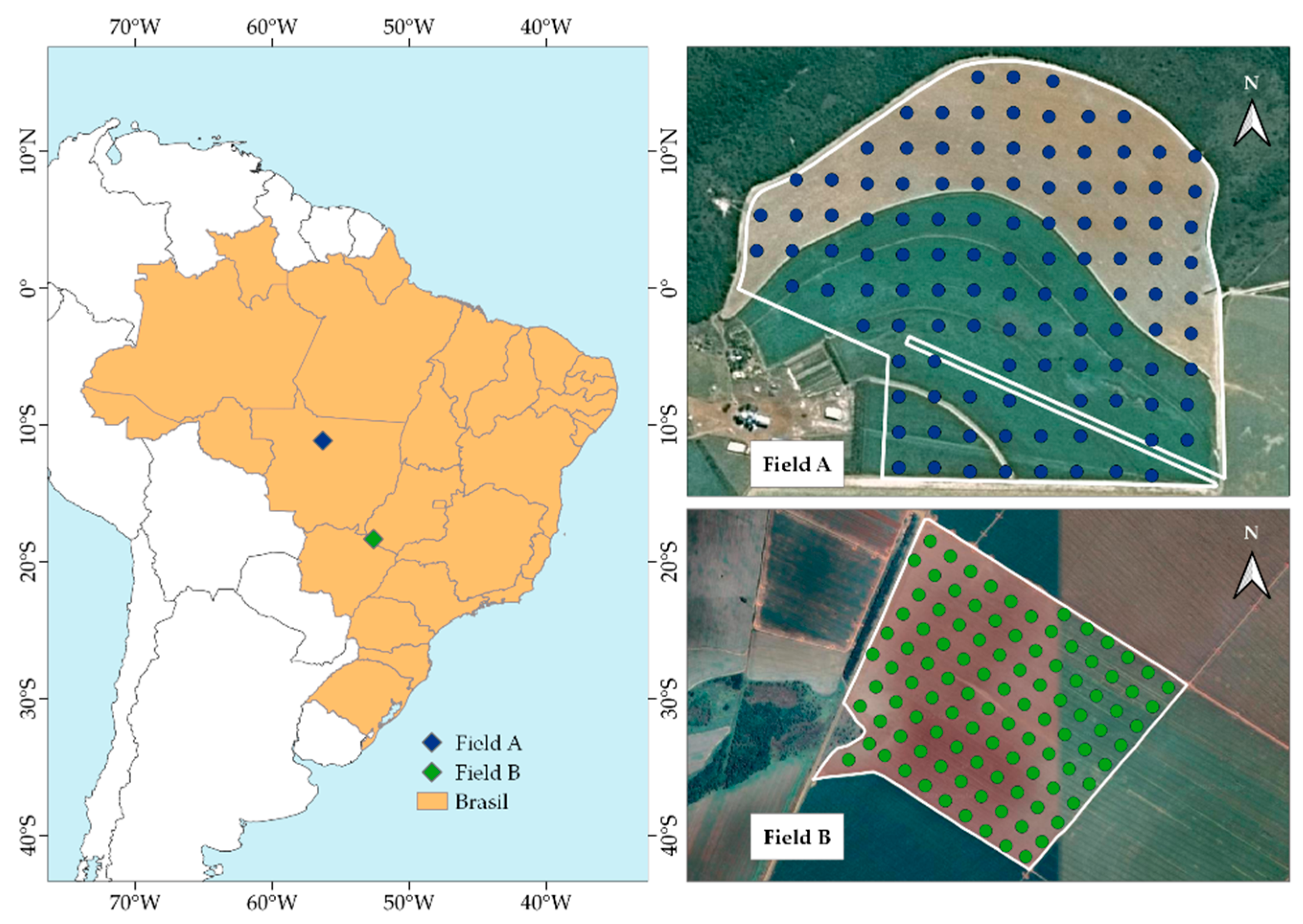
Figure 2.
Sampling methods defined by cells (CEL) and random cells (CEL-RND) for the study areas (Field A and Field B). The number within each zone represents its area in hectares.
Figure 2.
Sampling methods defined by cells (CEL) and random cells (CEL-RND) for the study areas (Field A and Field B). The number within each zone represents its area in hectares.
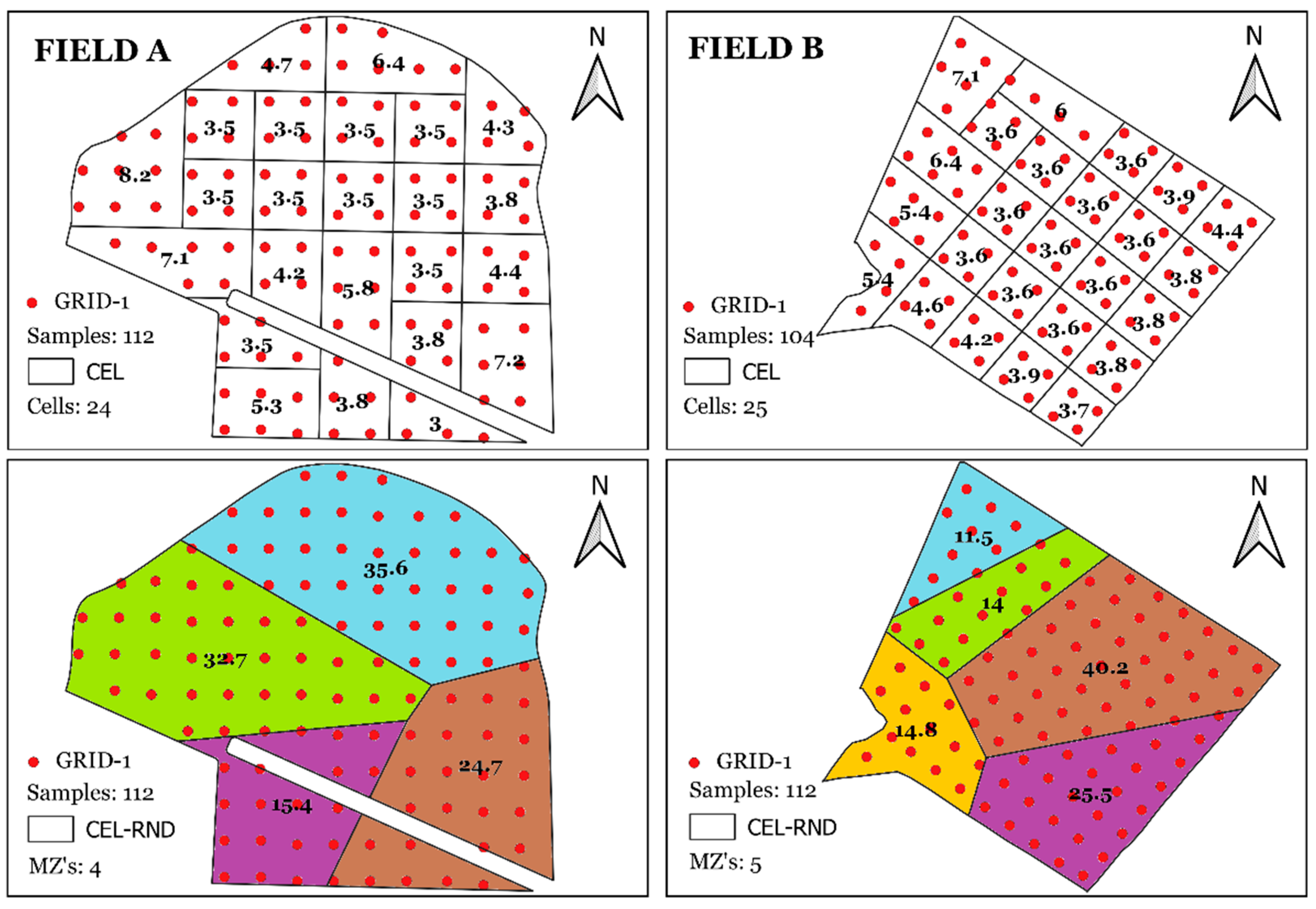
Figure 3.
Pearson correlation between VV (Vertical-Vertical polarization) and VH (Vertical-Horizontal polarization) backscatter values and SAR indices obtained in Fields A and B. VH: Vertical-Horizonal polarization; VV: Vertical-Vertical polarization; PRVI: Polarimetric Radar Vegetation Index; RVI4SI: Sentinel-1 Radar Vegetation Index; RVI: Radar Vegetation Index; NRPB: Normalized Ratio Procedure Between Bands; VV/VH: VV VH Ratio; VH/VV: VH VV Ratio.
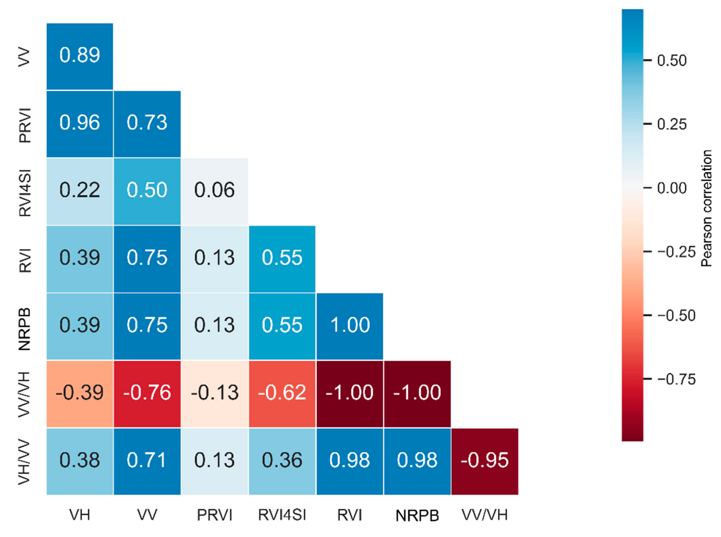
Figure 4.
Scatter plots with smoothed lines of backscatter coefficients and SAR indices for Fields A and B over the months, covering the period from January 1, 2018, to December 31, 2022. VV: Vertical-Vertical polarization; VH: Vertical-Horizonal polarization; VV/VH: VV VH Ratio: RVI4SI: Sentinel-1 Radar Vegetation Index.
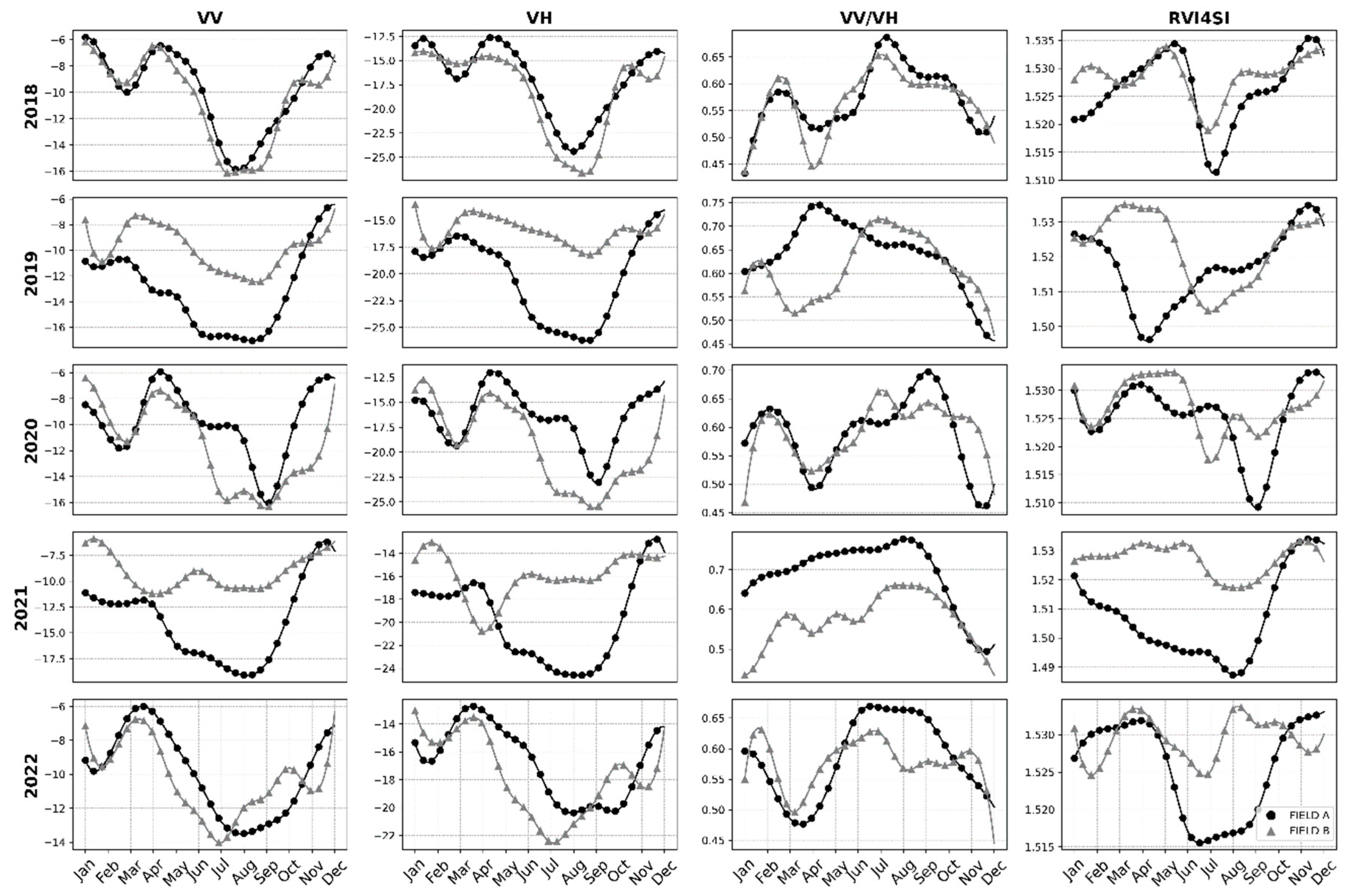
Figure 5.
Scatter plots with smoothed trend lines of monthly accumulated precipitation for Fields A and B, using NASA POWER data, in annual subplots from January 2018 to December 2022.
Figure 5.
Scatter plots with smoothed trend lines of monthly accumulated precipitation for Fields A and B, using NASA POWER data, in annual subplots from January 2018 to December 2022.
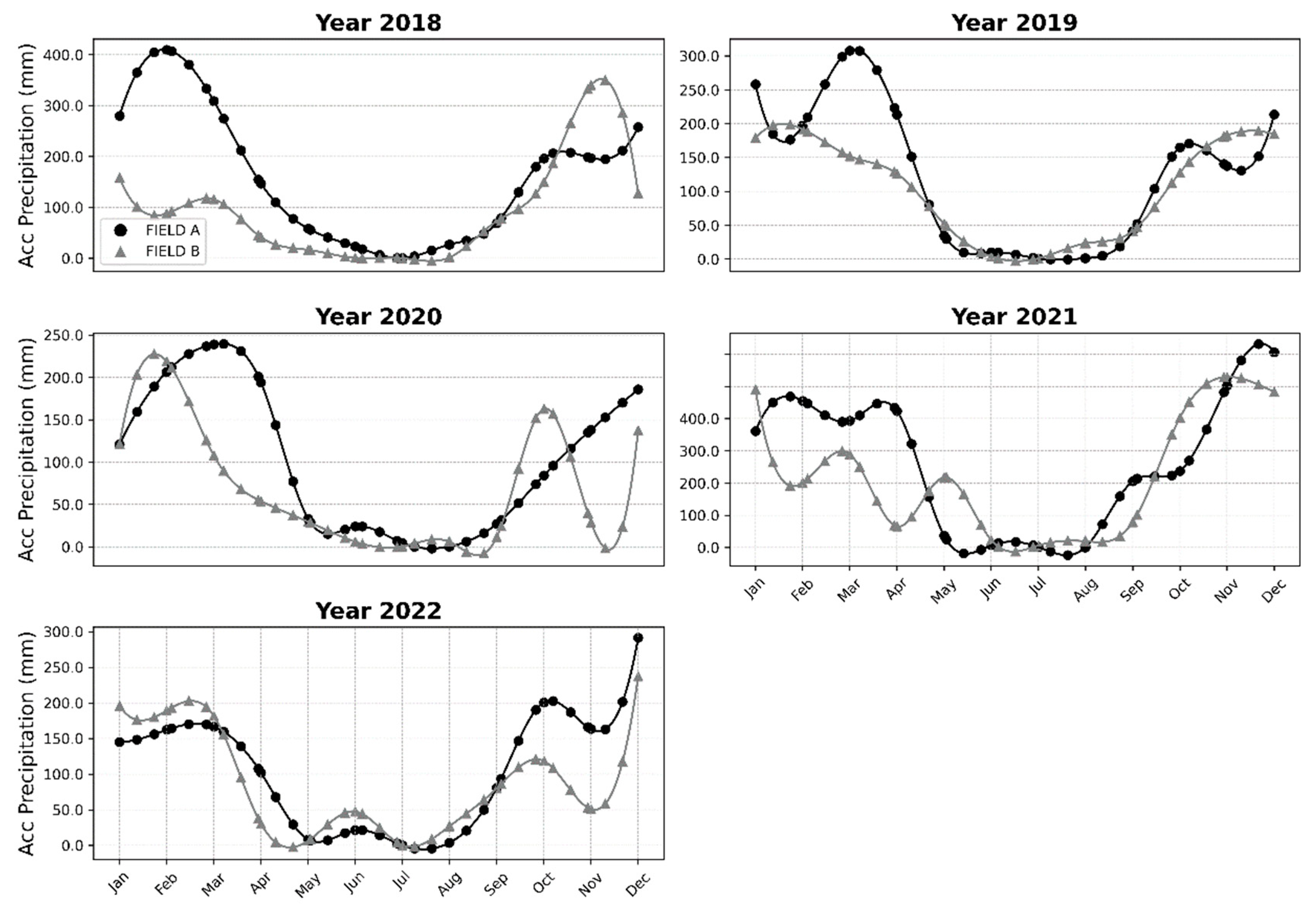
Figure 6.
Figures of soil attributes interpolated by ordinary kriging for Field A using GRID-1. CLA: Clay; pH: Active Acidity in water; P: Phosphorus; K+: Potassium; Ca2+: Calcium; Mg2+: Magnesium; C: Soil Organic Carbon; V: Basis Saturations; H+ + Al3+: Potential acidity.
Figure 6.
Figures of soil attributes interpolated by ordinary kriging for Field A using GRID-1. CLA: Clay; pH: Active Acidity in water; P: Phosphorus; K+: Potassium; Ca2+: Calcium; Mg2+: Magnesium; C: Soil Organic Carbon; V: Basis Saturations; H+ + Al3+: Potential acidity.
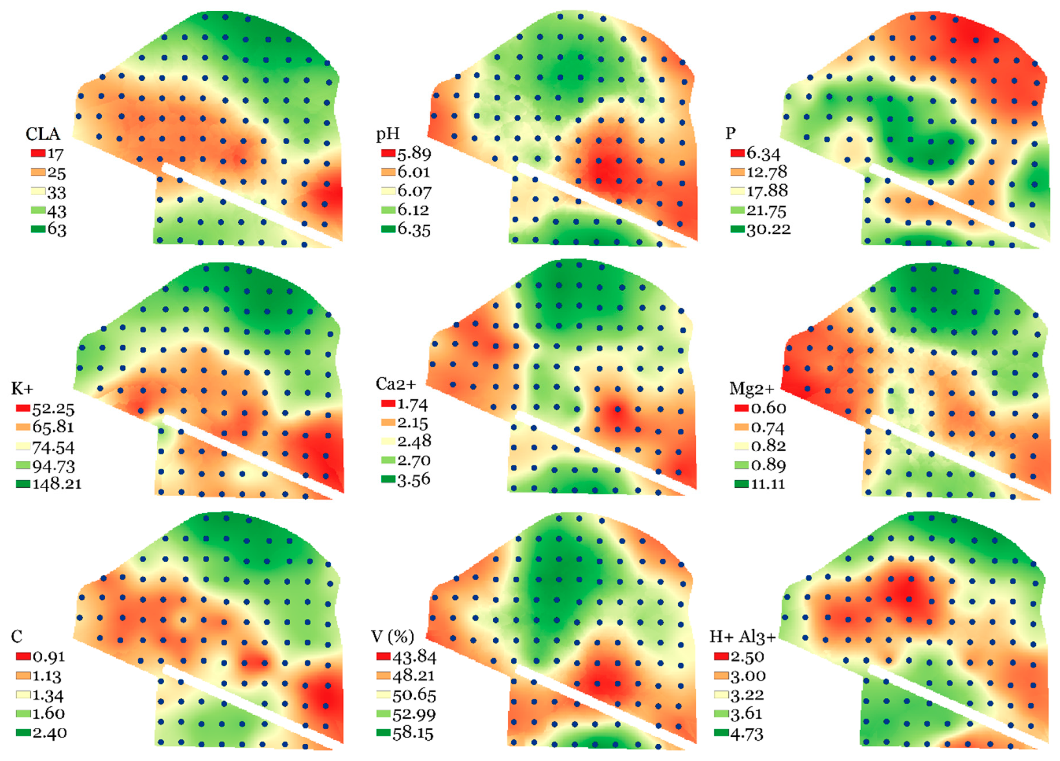
Figure 7.
Figures of soil attributes interpolated by ordinary kriging for Field B using GRID-1. CLA: Clay; pH: Active Acidity in water; P: Phosphorus; K+: Potassium; Ca2+: Calcium; Mg2+: Magnesium; C: Soil Organic Carbon; V: Basis Saturations; H+ + Al3+: Potential acidity.
Figure 7.
Figures of soil attributes interpolated by ordinary kriging for Field B using GRID-1. CLA: Clay; pH: Active Acidity in water; P: Phosphorus; K+: Potassium; Ca2+: Calcium; Mg2+: Magnesium; C: Soil Organic Carbon; V: Basis Saturations; H+ + Al3+: Potential acidity.
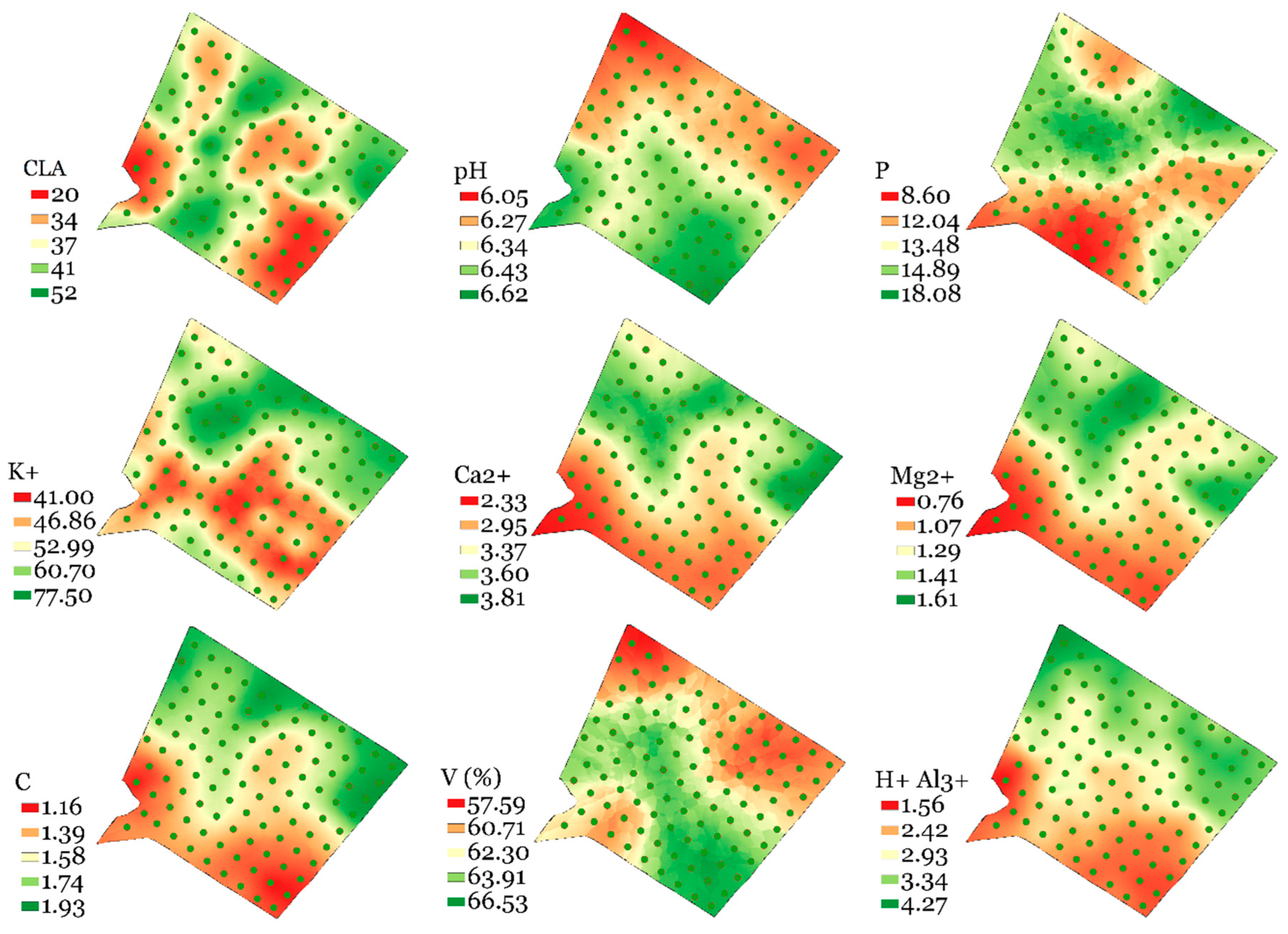
Figure 8.
Management zones resulting from SAR indices for both fields and approaches. The number within each zone represents its area in hectares. VV: Vertical-Vertical polarization; VH: Vertical-Horizonal polarization; VV/VH: VV VH Ratio: RVI4SI: Sentinel-1 Radar Vegetation Index.
Figure 8.
Management zones resulting from SAR indices for both fields and approaches. The number within each zone represents its area in hectares. VV: Vertical-Vertical polarization; VH: Vertical-Horizonal polarization; VV/VH: VV VH Ratio: RVI4SI: Sentinel-1 Radar Vegetation Index.
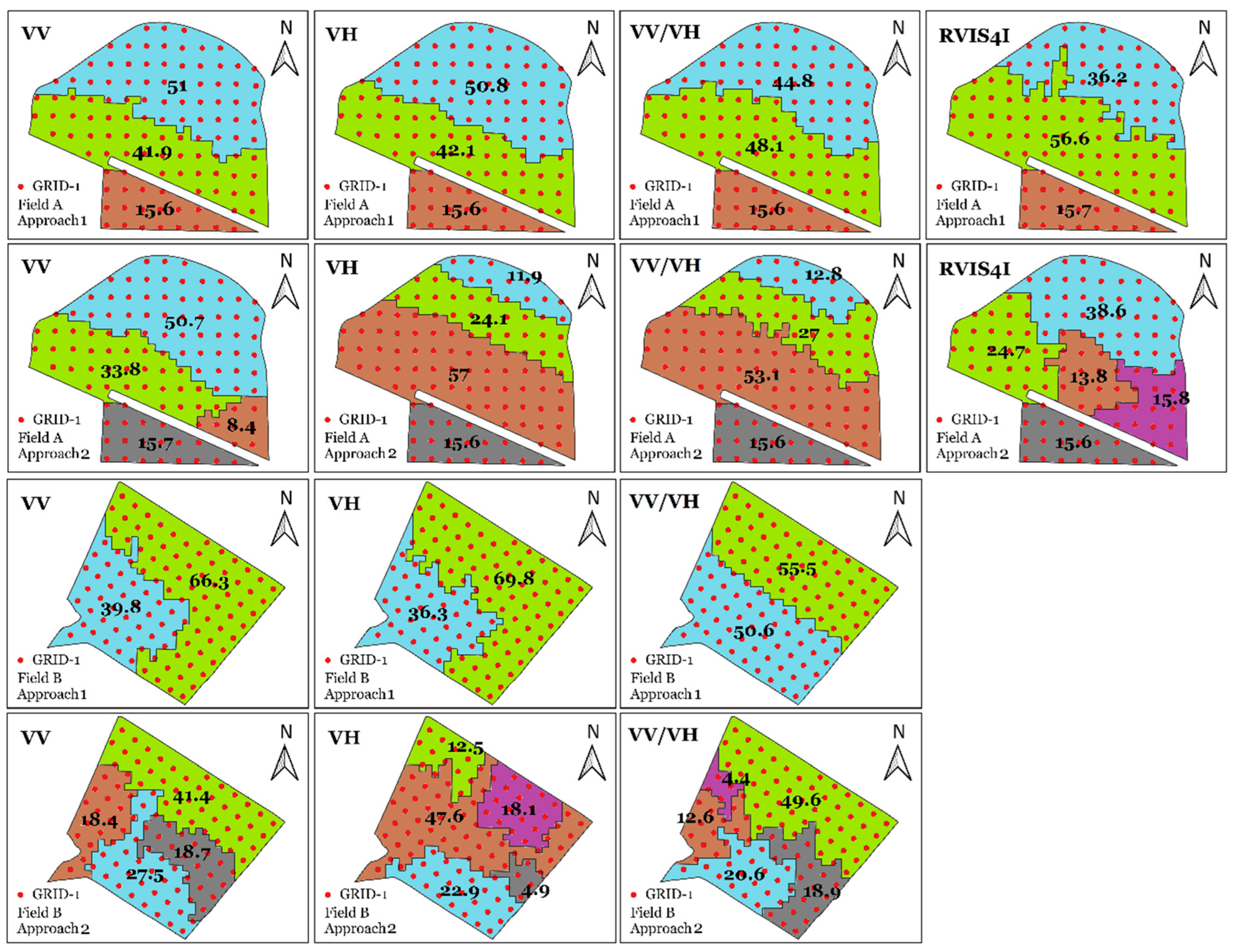
Figure 9.
The percentage value by which the RMSE of the Management Zones (MZs) soil sampling method, delineated by Approach 2 and the SAR VV/VH index, was greater than the RMSE generated by the 1000 random cell soil sampling method (CEL-RND) scenarios. CLA: Clay; pH: Active Acidity in water; P: Phosphorus; K+: Potassium; Ca2+: Calcium; Mg2+: Magnesium; C: Soil Organic Carbon; V: Basis Saturations; H+ + Al3+: Potential acidity.
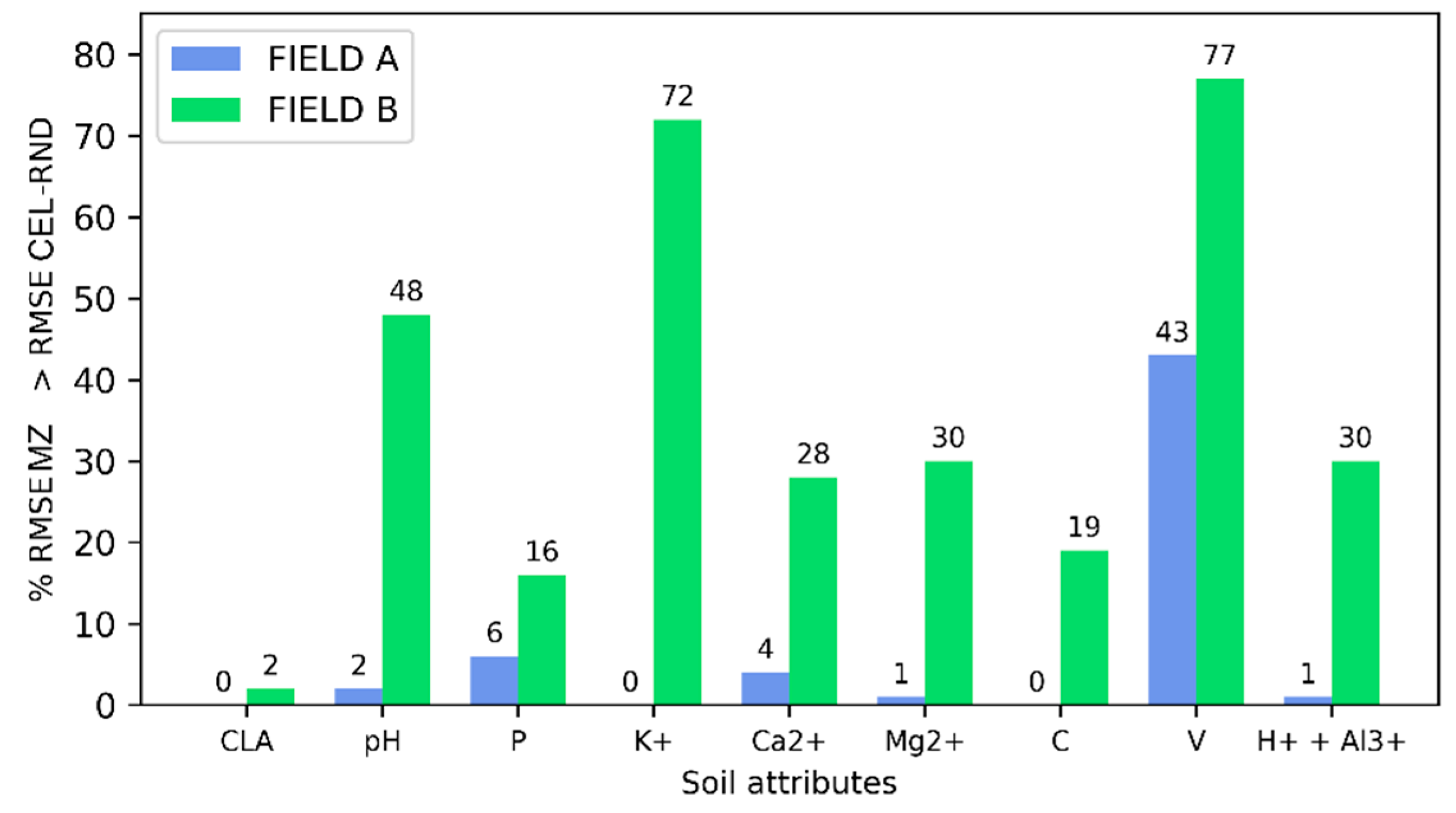

Table 1.
Summary of descriptive statistics of soil properties measured in the study area.
| Field | Soil attribute | Unity | Mean | Minimum | Maximum | STD | CV (%) |
| A | CLA | g/kg | 35.65 | 16.30 | 62.00 | 11.91 | 33 |
| pH | - | 6.11 | 5.76 | 7.78 | 0.28 | 5 | |
| P | mg/dm3 | 17.91 | 3.40 | 56.60 | 10.40 | 58 | |
| K+ | mg/dm3 | 86.24 | 25.00 | 199.00 | 36.72 | 43 | |
| Ca2+ | cmolc/dm3 | 2.55 | 0.99 | 5.82 | 0.70 | 28 | |
| Mg2+ | cmolc/dm3 | 0.84 | 0.43 | 1.68 | 0.22 | 26 | |
| C | cmolc/dm3 | 1.43 | 0.47 | 2.78 | 0.45 | 31 | |
| V | % | 51.65 | 36.70 | 97.00 | 8.95 | 17 | |
| H+ + Al3+ | cmolc/dm3 | 3.28 | 0.20 | 5.20 | 0.81 | 25 | |
| B | CLA | g/kg | 37.00 | 19.00 | 58.30 | 7.71 | 21 |
| pH | - | 6.35 | 5.81 | 6.91 | 0.21 | 3 | |
| P | mg/dm3 | 13.75 | 2.50 | 30.10 | 6.16 | 45 | |
| K+ | mg/dm3 | 55.55 | 26.0 | 120.00 | 19.43 | 35 | |
| Ca2+ | cmolc/dm3 | 3.30 | 2.14 | 5.23 | 0.61 | 18 | |
| Mg2+ | cmolc/dm3 | 1.25 | 0.72 | 2.08 | 0.29 | 24 | |
| C | cmolc/dm3 | 1.58 | 0.87 | 2.86 | 0.32 | 2 | |
| V | % | 62.29 | 49.50 | 74.60 | 5.46 | 9 | |
| H+ + Al3+ | cmolc/dm3 | 2.87 | 1.20 | 4.40 | 0.72 | 25 |
CLA: Clay; pH: Active Acidity in water; P: Phosphorus; K+: Potassium; Ca2+: Calcium; Mg2+: Magnesium; C: Soil Organic Carbon; V: Basis Saturations; H+ + Al3+: Potential acidity; STD: standard deviation; CV: coefficient of variation (%).
Table 2.
Specifications of the Sentinel-1 SAR data used in this study.
| Parameters | Specifications |
| Satellite Pass | Descending |
| Polarization | Vertical-Vertical (VV) Vertical-Horizontal (VH) |
| Speckle filter | Refined Lee - 3x3 (Lee et al., 1999) |
| Speckle filter Framework | Multitemporal – 10 images |
| Digital elevation model | NASA SRTM Digital Elevation 30m (T.G. Farr et al., 2007) |
SRTM: Shuttle Radar Topography Mission.
Table 3.
The SAR (Synthetic Aperture Radar) indices used in this study to delineate management zones.
Table 3.
The SAR (Synthetic Aperture Radar) indices used in this study to delineate management zones.
| Full Name | Abbreviated Name | Equation | Source |
| Polarimetric Radar Vegetation Index | PRVI | [38] | |
| Sentinel-1 Radar Vegetation Index | RVI4S1 | https://custom-scripts.sentinel-hub.com/custom-scripts/sentinel-1/radar_vegetation_index/# | |
| Radar Vegetation Index | RVI | [39] | |
| Normalized Ratio Procedure Between Bands | NRPB | [40] | |
| VV VH Ratio | VV/VH | [30] | |
| VH VV Ratio | VH/VV | [28] | |
| VH Backscattering | VH | - | |
| VV Backscattering | VV | - |
VV: Vertical-Vertical polarization; VH: Vertical-Horizonal polarization.
Table 4.
A proposed autoencoder architecture for feature extraction.
| Layers | Type | Neurons | Activation Function |
| Input Layer (SAR) | - | N° of SAR images each field | - |
| Encoder Layer 1 | Fully Connected | 32 | ReLU |
| Bottleneck Layer 1 | Fully Connected | 6 | ReLU |
| Decoder Layer 1 | Fully Connected | 32 | ReLU |
| Output Layer | Fully Connected | N° of SAR images each field | Sigmoid |
ReLU: Rectified Linear Unit; SAR: Synthetic Aperture Radar.
Table 5.
Parameters used to train the autoencoder architecture.
| Parameter | Value |
| Number of Epochs | 200 |
| Optimization Function | Adam |
| Learning Rate | 0.0001 |
| Batch Size | 1 |
| Loss Function | Mean Squared Error |
| Regularization | L2 (lambda = 0.01) |
Table 6.
O The theoretical model parameters were adjusted to the empirical semivariance of the soil attributes for Field A and Field B.
Table 6.
O The theoretical model parameters were adjusted to the empirical semivariance of the soil attributes for Field A and Field B.
| Field | Soil attribute | Model | Range (m) | C0 | C0 + C | R2 | SDI (%) | |
| A | CLA | Gaussian | 697.85 | 14.72 | 198.50 | 0.99 | 7.42 | |
| pH | Linear to Sill | 370.64 | 0.022 | 0.036 | 0.47 | 61.11 | ||
| P | Spherical | 396.95 | 45.27 | 96.66 | 0.74 | 46.83 | ||
| K+ | Linear to Sill | 642.51 | 286.77 | 1012.68 | 0.99 | 28.32 | ||
| Ca2+ | Linear to Sill | 419.14 | 0.12 | 0.36 | 0.79 | 33.33 | ||
| Mg2+ | Linear to Sill | 458.12 | 0.02 | 0.04 | 0.83 | 50.00 | ||
| C | Linear to Sill | 472.85 | 0.04 | 0.17 | 0.97 | 23,52 | ||
| V (%) | Linear to Sill | 347.48 | 28.78 | 48.47 | 0.59 | 59.37 | ||
| H+ + Al3+ | Linear to Sill | 379.13 | 0.24 | 0.57 | 0.67 | 42.11 | ||
| B | CLA | Spherical | 401.31 | 3.77 | 58.51 | 0.97 | 6.44 | |
| pH | Linear | 557.85 | 0.02 | 0.04 | 0.948 | 50.00 | ||
| P | Linear to Sill | 320.92 | 26.97 | 33.60 | 0.29 | 80.26 | ||
| K+ | Exponential | 788.23 | 160.36 | 341.29 | 0.92 | 46.99 | ||
| Ca2+ | Linear | 552.69 | 0.13 | 0.30 | 0.98 | 43.33 | ||
| Mg2+ | Linear | 559.91 | 0.03 | 0.08 | 0.99 | 37.50 | ||
| C | Linear | 557.18 | 0.03 | 0.09 | 0.99 | 33.33 | ||
| V | Linear to Sill | 585.78 | 23.10 | 31.00 | 0.96 | 74.19 | ||
| H+ + Al3+ | Linear | 569.48 | 0.09 | 0.53 | 0.98 | 16.98 | ||
CLA: Clay; pH: Active Acidity in water; P: Phosphorus; K+: Potassium; Ca2+: Calcium; Mg2+: Magnesium; C: Soil Organic Carbon; V: Basis Saturations; H+ + Al3+: Potential acidity; Range (m); C0: Nugget effect; C0 + C: Sill; R²: Coefficient of determination; SDI (%): Special Dependency Index.
Table 7.
RMSE of Approaches 1 and 2 for Fields A and B related to the VV and VH backscatter coefficients and the SAR indices VV/VH and RVI.
Table 7.
RMSE of Approaches 1 and 2 for Fields A and B related to the VV and VH backscatter coefficients and the SAR indices VV/VH and RVI.
| FIELD | Approach | Soil attribute | VV | VH | VV/VH | RVI4SI |
| A | Approach 1 | CLA | 8.99 | 9.01 | 7.82 | 7.67 |
| pH | 0.27 | 0.27 | 0.27 | 0.27 | ||
| P | 10.08 | 10.18 | 9.74 | 9.42 | ||
| K+ | 31.63 | 31.73 | 29.73 | 29.21 | ||
| Ca2+ | 0.66 | 0.65 | 0.65 | 0.65 | ||
| Mg2+ | 0.2 | 0.2 | 0.19 | 0.2 | ||
| C | 0.38 | 0.38 | 0.36 | 0.35 | ||
| V | 8.99 | 8.93 | 9.04 | 9.09 | ||
| H+ + Al3+ | 0.82 | 0.83 | 0.81 | 0.8 | ||
| Approach 2 | CLA | 8.33 | 6.34 | 5.74 | 7.82 | |
| pH | 0.27 | 0.27 | 0.27 | 0.27 | ||
| P | 9.98 | 9.81 | 9.67 | 10.02 | ||
| K+ | 31.28 | 24.87 | 23.7 | 29.47 | ||
| Ca2+ | 0.65 | 0.64 | 0.64 | 0.63 | ||
| Mg2+ | 0.19 | 0.19 | 0.19 | 0.19 | ||
| C | 0.36 | 0.3 | 0.27 | 0.35 | ||
| V | 9 | 9.08 | 9.05 | 8.99 | ||
| H+ + Al3+ | 0.82 | 0.75 | 0.75 | 0.83 | ||
| B | Approach 1 | CLA | 7.77 | 7.81 | 7.48 | - |
| pH | 0.21 | 0.21 | 0.19 | - | ||
| P | 6.24 | 6.23 | 6.21 | - | ||
| K+ | 19.24 | 18.79 | 18.28 | - | ||
| Ca2+ | 0.61 | 0.6 | 0.55 | - | ||
| Mg2+ | 0.29 | 0.29 | 0.26 | - | ||
| C | 0.32 | 0.31 | 0.29 | - | ||
| V | 5.51 | 5.52 | 5.3 | - | ||
| H+ + Al3+ | 0.7 | 0.7 | 0.56 | - | ||
| Approach 2 | CLA | 7.31 | 7.8 | 6.53 | - | |
| pH | 0.19 | 0.19 | 0.2 | - | ||
| P | 6.14 | 6.26 | 6.08 | - | ||
| K+ | 18.25 | 19.03 | 19.22 | - | ||
| Ca2+ | 0.57 | 0.57 | 0.53 | - | ||
| Mg2+ | 0.27 | 0.27 | 0.25 | - | ||
| C | 0.29 | 0.29 | 0.28 | - | ||
| V | 5.31 | 5.31 | 5.52 | - | ||
| H+ + Al3+ | 0.58 | 0.59 | 0.58 | - |
CLA: Clay; pH: Active Acidity in water; P: Phosphorus; K+: Potassium; Ca2+: Calcium; Mg2+: Magnesium; C: Soil Organic Carbon; V: Basis Saturations; H+ + Al3+: Potential acidity; VV: Vertical-Vertical polarization; VH: Vertical-Horizonal polarization; VV/VH: VV VH Ratio: RVI4SI: Sentinel-1 Radar Vegetation Index.
Table 8.
Univariate analysis of variance of soil attributes for the management zones delineated by Approach 2 and the SAR VV/VH index for fields A and B.
Table 8.
Univariate analysis of variance of soil attributes for the management zones delineated by Approach 2 and the SAR VV/VH index for fields A and B.
| Field | Management zones | Number of Samples | Soil Attributes | ||||||||
| CLA | pH | P | K | Ca2+ | Mg2+ | C | V | H+ + Al3+ | |||
| A | MZ1 | 20 | 38.11 | 6.29 | 19.81 | 73.35 | 2.91 | 0.87 | 1.47 | 54.40 | 3.34 |
| MZ2 | 52 | 25.97 | 6.02 | 21.41 | 67.38 | 2.20 | 0.72 | 1.12 | 49.84 | 3.04 | |
| MZ3 | 12 | 58.23 | 6.05 | 8.48 | 160.50 | 3.11 | 1.09 | 2.29 | 50.03 | 4.33 | |
| MZ4 | 28 | 42.18 | 6.15 | 14.13 | 98.64 | 2.70 | 0.93 | 1.59 | 53.75 | 3.23 | |
| Variance analysis | F-Value | 128.50 | 5.25 | 7.98 | 57.93 | 11.57 | 17.78 | 69.34 | 2.03 | 10.15 | |
| Prob > F | 0 | 0 | 0 | 0 | 0 | 0 | 0 | 0.11 | 0 | ||
| B | MZ1 | 49 | 39.30 | 6.26 | 14.54 | 62.08 | 3.60 | 1.41 | 1.73 | 60.94 | 3.31 |
| MZ2 | 4 | 40.58 | 6.28 | 16.7 | 55.00 | 3.80 | 1.54 | 1.75 | 63.32 | 3.18 | |
| MZ3 | 14 | 33.75 | 6.42 | 14.61 | 52.5 | 3.16 | 1.15 | 1.48 | 63.9 | 2.56 | |
| MZ4 | 20 | 40.58 | 6.42 | 9.63 | 48.85 | 2.98 | 1.06 | 1.44 | 62.92 | 2.45 | |
| MZ5 | 17 | 28.01 | 6.51 | 14.92 | 47.24 | 2.81 | 1.03 | 1.33 | 63.91 | 2.25 | |
| Variance analysis | F-Value | 12.80 | 6.89 | 3.13 | 3.07 | 11.21 | 13.86 | 9.14 | 1.57 | 16.57 | |
| Prob > F | 0 | 0 | 0.02 | 0.02 | 0 | 0 | 0 | 0.19 | 0 | ||
CLA: Clay; pH: Active Acidity in water; P: Phosphorus; K+: Potassium; Ca2+: Calcium; Mg2+: Magnesium; C: Soil Organic Carbon; V: Basis Saturations; H+ + Al3+: Potential acidity. CLA in g/kg; P e K+ in mg/dm3; Ca2+, Mg2+, C e H+ + Al3+ in cmolc/dm3.
Table 9.
RMSE of the sampling methods GRID-1, CONV, CEL, and MZs delineated by Approach 2 and the SAR index VV/VH for soil attributes in Fields A and B.
Table 9.
RMSE of the sampling methods GRID-1, CONV, CEL, and MZs delineated by Approach 2 and the SAR index VV/VH for soil attributes in Fields A and B.
| Field | Soil attribute | GRID-1 | CONV | CEL | MZs |
| A | CLA | 3.49 | 11.97 | 6.24 | 5.74 |
| pH | 0.22 | 0.28 | 0.29 | 0.27 | |
| P | 6.72 | 10.44 | 10.23 | 9.67 | |
| K | 18.59 | 36.88 | 25.32 | 23.7 | |
| Ca2+ | 0.43 | 0.71 | 0.64 | 0.64 | |
| Mg2+ | 0.15 | 0.22 | 0.2 | 0.19 | |
| SOC | 0.17 | 0.45 | 0.31 | 0.27 | |
| V | 7.07 | 8.99 | 9.34 | 9.05 | |
| H+AL | 0.55 | 0.82 | 0.84 | 0.75 | |
| B | CLA | 1.45 | 7.75 | 6.35 | 6.53 |
| pH | 0.14 | 0.21 | 0.2 | 0.2 | |
| P | 5.24 | 6.19 | 6.95 | 6.08 | |
| K | 12.69 | 19.52 | 20.12 | 19.22 | |
| Ca2+ | 0.36 | 0.61 | 0.46 | 0.53 | |
| Mg2+ | 0.14 | 0.3 | 0.2 | 0.25 | |
| SOC | 0.19 | 0.32 | 0.26 | 0.28 | |
| V | 4.63 | 5.48 | 5.66 | 5.52 | |
| H+AL | 0.26 | 0.72 | 0.54 | 0.58 |
CLA: Clay; pH: Active Acidity in water; P: Phosphorus; K+: Potassium; Ca2+: Calcium; Mg2+: Magnesium; SOC: Soil Organic Carbon; V: Basis Saturations; H+ + Al3+: Potential acidity. GRID-1: uniform grid soil sampling method; CONV: conventional soil sampling method; CEL: cell soil sampling method; MZs: management zone soil sampling method.
Disclaimer/Publisher’s Note: The statements, opinions and data contained in all publications are solely those of the individual author(s) and contributor(s) and not of MDPI and/or the editor(s). MDPI and/or the editor(s) disclaim responsibility for any injury to people or property resulting from any ideas, methods, instructions or products referred to in the content. |
© 2025 by the authors. Licensee MDPI, Basel, Switzerland. This article is an open access article distributed under the terms and conditions of the Creative Commons Attribution (CC BY) license (http://creativecommons.org/licenses/by/4.0/).
Copyright: This open access article is published under a Creative Commons CC BY 4.0 license, which permit the free download, distribution, and reuse, provided that the author and preprint are cited in any reuse.


