Submitted:
17 April 2025
Posted:
17 April 2025
You are already at the latest version
Abstract
The spatial distribution of ephemeral and perennial dryland plant species is increasingly modified and restricted by ever-changing climates and development expansion. At the interface of biodiversity conservation and developmental planning in desert landscapes in the growing need for adaptable tools in identifying and monitoring these ecologically fragile plant assemblages, habitats and, often, heritage sites. This study evaluates usage of Sentinel-2 time-series composite imagery to discriminate vegetation assemblages in a hyper-arid landscape. Spatial predictor spaces were compared to classify different veg-etation communities: spectral components (PCs), vegetation indices (VIs), and their combination. Further, the uncertainty in discriminating field-verified vegetation as-semblages is assessed using the Shannon entropy and intensity analysis. Lastly, the intensity analysis helped to decipher and quantify class transitions between maps from different spatial predictors. We mapped plant assemblages in 2022 from combined PCs and VIs at overall accuracy of 82.71% (95% CI: 81.08, 84.28). A high overall accuracy did not directly translate to high class prediction probabilities. Prediction by spectral com-ponents, with comparably lower accuracy (80.32, 95% CI: 78.60, 81.96), showed lower class uncertainty. Class disagreement or transition between classification models was mainly contributed by class exchange (a component of spatial allocation) and less so from quantity disagreement. Different artefacts of vegetation classes are associated to the predictor space - spectral components versus vegetation indices. We contribute insights into using feature extraction (VIs) versus feature selection (PCs) for pixel-based classification of plant as-semblages. Emphasising the ecologically sensitive vegetation in desert landscapes, the study contributes uncertainty considerations in translating optical satellite imagery to vegetation maps of arid landscapes. These are perceived to inform and support vegetation map creation and interpretation for operational management and plant conservation in such landscapes.
Keywords:
Sentinel-2 Dense time series
; Desert plant assemblages
; Forward Feature Selection
; Random Forest Ensemble Classifier
; Spatial cross-validation
; Shannon entropy
; Intensity Analysis
1. Introduction
Dryland vegetation communities endure remarkable ecological resilience and adaptation strategies that are increasingly challenged by uncertain climate patterns and changing ecological conditions. Globally, drylands comprising arid and hyper-arid regions has been estimated at 27% of the terrestrial surface area [1]. Local scale mapping and conservation of, often heritage and ecologically unique, arid plant communities is gaining global attention considering the upsurge in developmental actions that undermine the spatial and temporal shifts in plant habitats due to changing climates. The differentiation of environmental conditions at local scale is an important determinant of plant biodiversity and distribution [2,3]. Such differentiation, mediated by variability in topography, promotes the formation of micro-refugia for plant species [4] – stressing the importance of microtopographic variability. Variability in the spatial configuration of terrain contributes to diversifying potential plant habitats, on one hand. On another, by decreasing the spatial range of individual habitats and their likely connectivity, it mitigates inter-species competition (for limited space and resources); thus, contributing to plant micro-refugia and species’ richness [4,5,6]. The mapping of these refugia and vegetation assemblages is imperative in monitoring spatial changes and in planning the protection and conservation of their contributed and heritage biodiversity.
Land use and land cover maps, by and large, are increasing serving as support tools for both research and end-user applications as predicting impacts of climate crisis and planning development or management strategies [7,8,9,10]. Since maps are a simplified representation of ground reality, errors and uncertainties are inevitable in their production. These errors vary in magnitude depending on one of several, often compounding, factors including data quality, data processing, and analysis procedure [11]. Thus, an important consideration of such maps is their reliability or uncertainty – often evaluated by metrics of map quality or accuracy. For effective remote sensing application, different approaches have been suggested for accounting and reporting uncertainties in classification at the pixel level [12], object-based [13,14,15] and scale-based or spatial uncertainty [16,17]. In general, different analysis and target application of land use and land cover, whether pixel- or object-based, warrant corresponding scale of accuracy assessment [18]. Thus, approaches combining multi-features (several indices, texture) at high spatiotemporal resolution are promising in differentiating classes of mixed vegetation or land cover [19,20,21,22], which may inform several intended conservation and management endeavours in drylands and desert landscapes.
In remote sensing of vegetation, the use of Vegetation Indices (VIs) have been largely successful in mapping high and dense vegetation landscapes [19,22]. Such vegetation retain leaf and related phenological cycles over prolong periods, which feeds sensitivity of VIs and other proxies as feature texture. Leaf phenology and texture is captured in aerial or satellite images and across time series to inform the differentiation and mapping of different and mixed vegetation [15,21,22,23,24]. However, such proxies of vegetation may be applicable and reliable in arid and desert landscapes to a lesser extent. In arid and desert landscapes, permanent vegetation prevails in cultivated farms and active oases, in existent montane forests, sparse woodlands. A considerable proportion of the vegetation has ephemeral distribution, with very brief periods of green leaf phenology – chlorophyll retention – during periods of rainfall and water flushes into the Wadis (water channels and catchments). Since these periods of vegetation proliferation are often erratic and short-live, field observations of vegetation occurrence and distribution may not be readily reflected in remote sensing-based proxies of vegetation status. And, these proxies may be less sensitive, or the lack thereof, to observed non-green, dried, and sparse vegetation [25,26,27]. Thus, it is unrealistic to continuously apply classic proxies and assumptions, mostly reliable to permanent vegetation distribution and density, in mapping vegetation in arid and desert landscapes. Usage of spectral-based VIs, as spatial predictors, to map and monitor arid vegetation is increasingly questionable [11,26,28] and may be unreliable for different and specific landscapes [11,20,25,27,29,30,31]. Thus, for brief and mostly dry vegetation in arid landscapes, it is unreasonable to continuously apply or assume unverified reliance on Vegetation Index (VI) proxy from multi-spectral remote sensing data. Such proxy may be reliable under certain landscape specifics – such as in areas with persistent vegetation cover - and in other circumstances provide only complementary information in discriminating vegetation assemblages and mapping their distribution.
The spatial and temporal heterogeneity of dryland vegetation are key contributors to errors in mapping their distribution. Nonetheless, literature on remote sensing of such vegetation has overlooked quantifying the uncertainties in vegetation mapping from spatial features of spectral signatures and vegetation indices. Different methods have been suggested in assessing accuracy or errors of remote sensing classification of vegetation and land cover at the pixel-based level [32,33], local spatial scale [34], object-based feature extraction [35], and map change classification [36,37]. In addition to classification error and confusion, spatial consideration of unknown space, for which no reference predictor information is available, is essential in estimating area of applicability of map outputs [16,17]. The application of remote sensing in pixel-based (soft) classification produces errors that vary across space. Thus, usage of overall accuracy estimates, and related metrics as kappa, provide less intuitive visual clues to, and interpretation of, the spatial variability and patterns in classification errors [32,38].
Uncertainties in mapping vegetation have been largely overlooked in remote sensing of vegetation in arid, semi-arid and desert landscapes [39,40,41,42]. There is scant literature that either validate or benchmarks the reliability and spatial extent of VIs-based mapping of desert plant communities for applications as biodiversity conservation and development planning. This study, therefore, questions and dissociates, based on quantified classification uncertainties and spatial disagreement, the contribution of VIs proxies versus principal spectral information in discriminating and mapping vegetation assemblages in desert landscapes. Using a dense time-series of Sentinel-2 imagery and the random forest (ensemble features) classification algorithm, we quantify classification error from both per-pixel class uncertainty by Shannon entropy (information loss) and feature-based uncertainty by intensity analysis of class transition across classification models.
2. Materials and Methods
2.1. Study Area
The study landscape is Wadi Ashar in AlUla County (in Al Madinah District) of the Kingdom of Saudi Arabia. The landscape’s physical structure and geology comprise a mix of several spectacular natural features and landforms (sandstone massifs, harrat plateaux, steep gorges, sand dunes, sandy plains, open Wadis, or seasonal drainage channels) and land uses (irrigated farms, date palm orchards, animal camps, etc.). The elevation across the landscape ranges between 760m a.s.l in the Wadis to 1240m a.s.l on the Harrat plateaus, while the terrains have slope range of 0 to 75 degrees. The administrative boundary covers a surface area of about 3,046 ha (Figure 2), and the landscape has established and planned development strategies and facilities of both public, touristic, and regal interests - exquisite hotel resorts. At its centre is the iconic Maraya Concert Hall as the centre structure of a developed chain of exquisite desert resorts which are punctuated by heritage landscape features and touristic attractions.
2.2. Vegetation Classification and Mapping
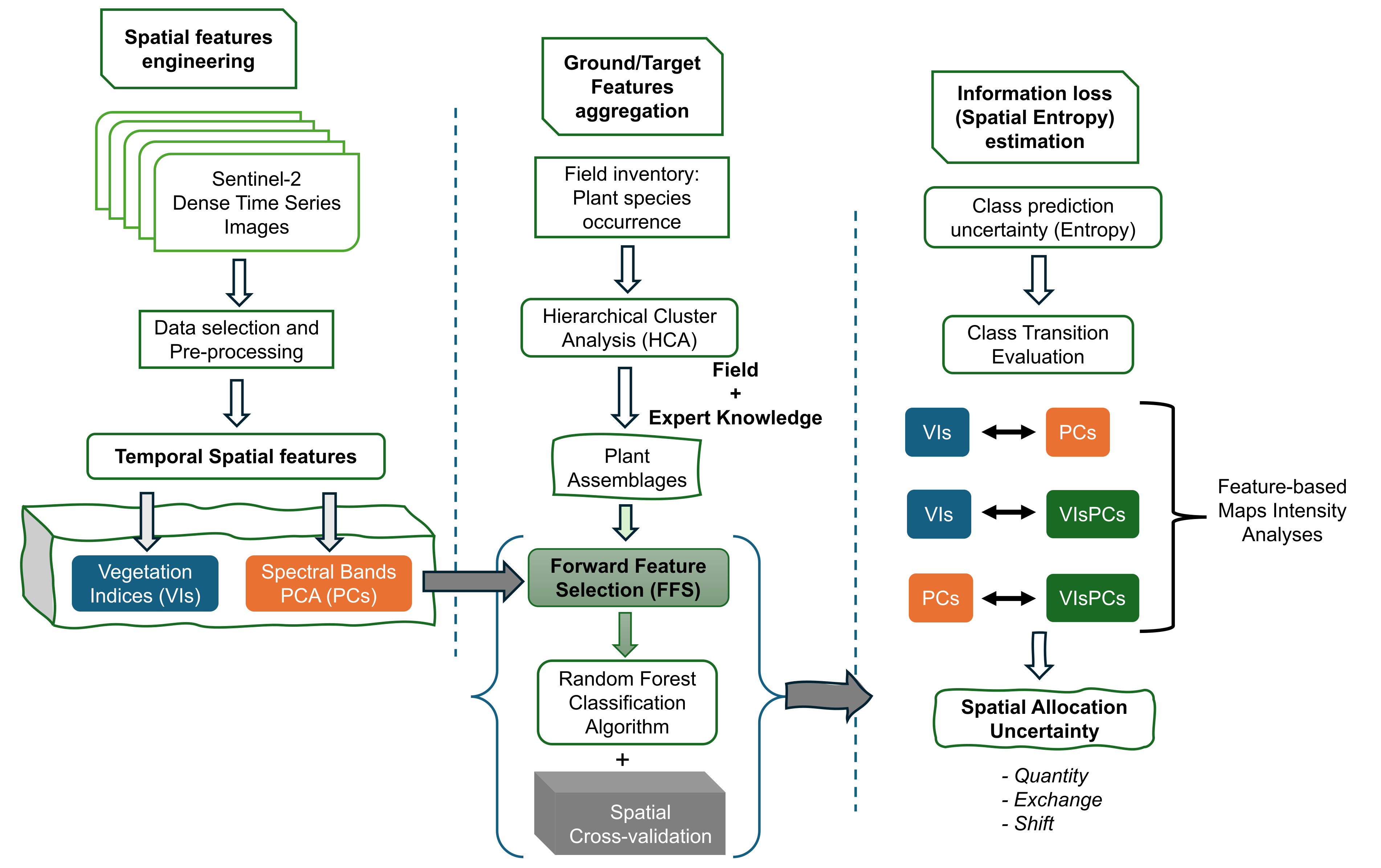
In detecting and mapping the different field-surveyed vegetation communities or assemblages, we implemented supervised classifications based on the random forest ensemble (bagging and decision tree) algorithm [43]. As predictors for the classifier algorithm, we explore spatial information of spectral bands and their derivative vegetation indices from time-series Sentinel-2 multi-spectral imagery. The details of the reference ground truth data, spatial data, and classification procedure are provided in the following subsections.
2.2.1. Plant Survey (Field) Data
Field data and observations are initially a mosaic of different key vegetation types in the study area. The vegetation types were preliminarily categorised into a high order based on three major habitats: sandy plains, sand dunes and harrats. To better understand these habitats and generate vegetation descriptions and maps, extensive field data were sampled during field surveys - the surveys were conducted from November to December 2021 and in September 2022. During the surveys, two types of plant data were collected: 1. Plot data - a complete list of the plants in a delimited plot of vegetation, with information on species cover, substrate, and other abiotic features; 2. General observations – to ensure that we capture as wide a variety of plant species found on the site as possible.
To ascertain and describe vegetation community on surveyed locations, which had associated identified plants, the plant species data, recorded as species abundance (values from 0 to 5 coded according to a DAFOR scale), were then subjected to hierarchical cluster analysis (HCA). The HCA helped define the reference classes or types of vegetation communities in the study area. Further visual observation in google earth enabled extracting additional reference points identified for roads, settlements, and other farms or agricultural areas. These, in addition to the vegetation survey points, serve as ground truth data (Table 1) for remote sensing data extraction and classification model training. The reference spatial data were extracted using reference polygons for the identified vegetation classes (described in Table A1 of online Supplementary Material).
2.2.2. Spatial Data and Processing
As spatial information, we explore Sentinel-2 (S-2) Multi-spectral Image archives provided by the European Space Agency. Available S-2 images covering the study areas were accessed using the Google Earth Engine (GEE) cloud computing platform, and the time-series images were filtered for images acquired for the area of interest in the period between 1st January 2021 to 15th September 2022 with cloudy pixel percentage of < 5% for each image. A total of 85 images (temporal series) were accessed following this filtering criteria, and each image collection was processed to compute 5 different vegetation indices (VIs) that provide proxy for vegetation status and cover: NDVI: Normalized Difference Vegetation Index [44], EVI: Enhanced Vegetation Index [45,46,47]. SAVI: Soil Adjusted Vegetation Index [48], MSAVI2: Modified Soil-Adjusted Vegetation Index – 2 [49] and GSAVI: Green Soil Adjusted Vegetation Index [50]. For each computed VI, we estimated and retained the max values for each pixel across the time-series [51]. Thus, the pre-processing of spatial data resulted in 5 raster images for the vegetation indices.
In addition to spatial information from VIs, we explored information lurking in the spectral signatures (for both vegetation and non-vegetation) to potentially improve the classification based on VIs. For each of the computed VI, we extracted the corresponding spectral bands to create a raster stack of spectral signatures. A total of 20 spectral bands (4 from each VI corresponding to the Blue, Green, Red, and Near Infrared bands) were subjected to a Principal Component Analysis (PCA) data reduction procedure to obtain a set of uncorrelated spatial features. Based on the PCA, 5 Principal Components (PCs) explained about 99% of the variance in the spectral signatures for the study area (Table 2), of which 4 were most significant [52]. The PCs (raster layers) estimation procedure is illustrated in Figure 3. The PCs raster layers served as additional explanatory variables for vegetation and land cover classification. Thus, in total, we used 10 raster layers (5 PCs and 5 VIs) as the spatial predictors or environmental space for vegetation classification.
2.2.3. Vegetation Type Classification and Validation
To map the vegetation assemblages (and land cover) in study landscapes, the random forest classification algorithm was implemented to delineate clusters of vegetation types, hitherto identified, and grouped as clusters of plant assemblages. The reference polygons for the vegetation assemblages or land cover classes (Table 1) were used to extract training data from the stack of raster layers (10 explanatory or predictor raster in total). Considering disparities in both the number and size of reference polygons for each class, the extracted training data or pixels were unbalanced across the considered classes.
We trained Random Forest classification models to learn distinguishing features of plant assemblages based on the ten (10) raster predictors. Considering the unbalanced tally of reference clusters and extracted spatial data between the target vegetation and land cover classes, we tuned the hyper-parameters for the random forest classification algorithm by applying forward feature selection (FFS) and spatial cross-validation procedures [16]. We used a spatial 5-fold cross-validation (k = 5), and the ground truth data had the minimum of 5 reference polygons for the “Bare rock” class; thus, ensuring each fold in cross-validation contains data from each reference class. Based on the unique IDs for each reference polygon, we implemented a spatial cross-validation, using the Leave-Location-Out Cross-Validation (LLO-CV) procedure, which specify that data from the same polygon are always grouped prevent usage in both model training and testing [16] procedure by leaving location out at each iteration of model training.
2.2.4. Classification Error and Area of Applicability
Using Dissimilarity Index (DI) in assessing the area of applicability (AOA) of the final classification map. As suggested by [16], we considered areas with predictor space (VI and Spectral features) that are unknown to the classification model are termed “Unknown spaces” and identified by high Dissimilarity Index. The dissimilarity index was computed based on weighted distance of new prediction space and the average (threshold) distance within the spatial cross-validated prediction space in the trained model. Thus, for model prediction, areas, or pixels with a DI < Threshold were classified to be within the Area of Applicability (AOA) for model prediction. The predictions within the AOA were based on the DI map and threshold (Figure 4).
2.3. Quantifying Uncertainty (Information) in Class Prediction
There is an unreliable common practice in remote sensing literature to overlook details of sampling scheme and size for accuracy assessment [18]. This is especially the case for object-based image analysis (OBIA) and less likely so for pixel-level classifications. To ascertain and delineate the contribution of spectral signature versus vegetation indices to discriminate vegetation assemblages, we compare three models or scenarios of predictor (explanatory) remote sensing variables: 1) Model VIs: Using vegetation indices (VIs) – 5 raster images, 2) Model PCs: Using principal components (PCs) of time-series spectral signatures – 5 raster images, and 3) Model VIsPCs: Using both VIs and PCs as predictor features – 10 raster images.
In quantifying the uncertainty in the pixel-based classification, a measure of uncertainty, the Shannon Entropy (H), computed from predicted class probability, was applied to evaluate information gained from the use of different spatial predictors. For pixel-based classification, the Shannon entropy or cross-entropy has been applied in remote sensing for edge detection [53], in measuring of class error [21], in quantifying land use change and dynamics [54,55,56].
The entropy of a random variable, according to information theory [57], is the average level of "information", "surprise", or "uncertainty" inherent to the variable's possible outcomes. Given a discrete random variable X, which takes values in the alphabet X and is distributed according to p: X → [0,1], the Shannon Entropy (information content, surprisal, or self-information) is estimated as follows:
where: H(X) is the total amount of information in an entire probability distribution, p(xi) is probability of classifying a pixel as class i, log is logarithm, and b is the base of the log and changing its value modifies the unit of estimated entropy. The choice of base for log, the logarithm, depends on the applications: base 2 = unit of bits or "Shannon" unit, base e = "natural units" nat, and base 10 = units of "dits" or "bans".
To ascertain the level of information or uncertainty in class predictions, the Shannon entropy was employed as a measure of the reliability in the predicted probabilities (class votes) by the random forest ensemble models. The estimated Shannon entropy (uncertainty) was compared between classes and across the different models (predictor features). To evaluate the within-class variability in uncertainty, we applied the Kernel density (distribution) profiles and non-parametric Kruskal-Wallis test with mean comparison based on Dunn test pairwise comparison and Bonferroni p-value adjustment.
2.4. Dissociating the Contribution of Predictor Features: Intensity Analysis
Intensity analysis provides a procedure for analysing land use change and transition at three different levels: time interval, category, and transition level [58,59,60]. The three successive levels of analysis form a hierarchical framework to decipher increasing details in change patterns at specific time intervals (or between maps) and assuming that the spatial extent is identical at each time point and class categories between comparable maps. To assess class uncertainty and accuracy between the three classification models, we apply the categorical and transition level intensity analysis.
The category level intensity analysis examines how the loss intensity, Lti, from category i and the gain intensity, Gtj, to category j compares to a uniform intensity, St, during each map interval [Mt, Mt+1]. If Lti < St, then Lti is dormant i.e. category i experiences loss less intensively than if the change during map interval [Mt, Mt+1] were uniformly distributed across the spatial extent. If Lti > St, then Lti is active, implying that category i experiences loss more intensively than if the change during map interval [Mt, Mt+1] had uniform distribution across the analysis domain or spatial extent of map. Likewise for the gain intensity, if Gtj < St, then Gtj is dormant; and Gtj is active when if Gtj > St. The computation of St, Lti and Gtj is illustrated in Eq. (3), Eq. (4) and Eq. (5), respectively.
At the transition level, the analysis examines how the transition intensity, Rtij, from category i to category j compares to a uniform transition intensity Wtj given the gain of category j during interval [Mt, Mt+1]. If Rtij < Wtj, then the gain of j transitions from i less intensively during time interval [Mt, Mt+1] than if the gain of j were to have transitioned uniformly from the space that is not j at time Mt - i.e. the gain of j avoids i. Conversely, If Rtij > Wtj, this implies the gain of j transitions from i more intensively during time interval [Mt, Mt+1] than if the gain of j were to have transitioned uniformly from the space that is not j at time Mt i.e. the gain of j targets i. Equations (6) and (7) illustrate, respectively, estimates of Rtij and Wtj. The order of subscripts j and i in Ctji of the denominator of Eq. (7) allows that the summation over i subtracts category j at the initial time Mt. The relationship among the different equations and intensity estimates is illustrated in Table 3 and Table 4.
The conceptual organization of the various intensities and land use dynamic degrees during time intervals [Mt, Mt+1] is presented in Table 4. At the transition level, the intensity analysis determines if the gain of a category j either avoids or targets its transition from another category I; thus, the intensity analysis compares a uniform transition intensity (Wti) to its corresponding transition intensities within each column j, Rtij. For the category level analysis, a comparison is made between change percentage in the time interval St and both the loss intensities (Lti) and the gain intensities (Gtj) to determine whether each loss and gain is dormant or active.
3. Results
3.1. Vegetation and Land Cover Classification
Plant assemblages (or communities) were discriminated, based on time-series of both spectral information and vegetation indices, with reliable accuracy. Overall, the different vegetation types were predicted with an overall accuracy of 0.834 (95% CI: 0.8178, 0.8493), a kappa of 0.699, and a global F1-Score of 0.535 as detailed on Table 5. The classification error was within reported reasonable range in remote sensing of vegetation in arid landscapes [41,65,66]. However, there was high variability in individual class accuracy across different classification models. All the models showed a high specificity and sensitivity in discriminating the monoculture farmlands and orchards (Table 6). For mixed plant assemblages, the classification uncertainty and accuracy were variable between the different models. The thematic map of 11 vegetation and land cover categories, including the unclassified areas – outside AOA, for the three classification models are depicted in Figure 5.
3.2. Classification Uncertainty
The Kernel density distribution, within the quantile range 2.5 to 97.5%, of the estimated Shannon entropy (classification uncertainty) for the vegetation categories is reported in Figure 6. A low classification uncertainty is observed for class representing mono-specific plant assemblages and/or their mosaic structure in farms or orchards (FO). For all the other considered categories, the distribution of the uncertainty is either skewed or multi-model across the different classification models (top row of Figure 6). Classification model based on vegetation indices (top middle panel in Figure 6) showed a normal distribution in the range of uncertainty (information complexity) for both uniform (FO) and high (VTW) vegetation categories. The range of statistics representing vegetation proxy and spectral information of the FO class was wide enough to reliably predict the spatial and structural variability in the class. In general, the kernel distribution of Shannon entropy (H) is indicative of high variability in classification uncertainty, for some vegetation assemblages, both in the pixel domain and local spatial levels. For the FO category, using VIs as predictor showed lowest uncertainty estimate (4.76%) in comparison to using the spectral components - PCs (6.13%) - and the combined predictors - VIsPCs (11.16%).
3.3. Change Intensity by Spectral information Versus Vegetation Indices
Overall differences in class quantity and allocation (exchange and shift) - between the classification models (maps) - are presenting in Figure 7. The exchange component represents allocation difference due to pairwise confusions while shift component estimates allocation difference from non-pairwise confusions. The class allocation components, exchange and shift, accounted most of the difference between all three thematic maps. Highest class disagreement was observed between the thematic maps from spectral components (PCs) and vegetation indices (VIs); compared to the latter, the former had lower allocation difference to map predictions based on combined predictors (VIsPCs). Although the overall accuracy of the VIs-based map was higher than that based on PCs predictors, the latter showed more consistency in discriminating other vegetation assemblages excepting farms and orchards. With reference to the combined (VIsPCs) model, the overall quantity disagreement in the PCs-based classification (7.60%) was less than that observed in the VIs -based classification (9.68%)., for the PCs to VIs map transition, the quantity component derives largely from a net gain of 2 non-vegetation categories - R and BR - and net loss in 2 vegetation categories - OVRW and OMSSS - (Figure 8). The contribution of such classes to the quantity component is backed by the heterogeneous nature and distribution of vegetation in the desert landscapes as modulated by major landforms and topography. Such spatial heterogeneity in vegetation and landforms is well captured in time-series image composite and the derived spatial features from principal (spectral) components.
The Land cover and use level change intensity between the map predictions is presented in Figure 8A. In general, we observed an active change intensity (gain and loss) for most classes across the different models. However, for some classes, large change intensity is attributable to their comparably small change area (size) in comparison (initial) map than in the reference map. Such as observed for the following classes: HSS, DSSDC, BGU, OutsideAOA. Figure 8B presents the three components of the quantified disagreement between reference and comparison maps: quantity, exchange, and shift. The components are stacked to highlight their respective contribution to overall class disagreement between the maps reference and comparison maps. In other words, their joint contribution conveys, for the purpose of this analysis, the proportion of correctly classified pixels (often calculated as 1 – total proportion of disagreement). Thus, uncertainty in class predictions based on spectral components versus vegetation indices centred around class allocation disagreements and less so from proportion correction (quantity disagreement).
4. Discussion
4.1. Vegetation Discrimination Accuracy
The classification models had accuracies in the range widely reported in remote sensing literature [18]. However, reliance on class accuracy to validate land use maps is a subject of increasing debate. Controversies in the acceptable range of classification accuracy hinge on complexities in validation related to (1) variability in mapping goals, (2) the errors of mapping as a function of the target classes, (3) heterogeneity within and between landscapes, and (4) the highly variable quality of remotely sensed data between classification experiments [68]. Thus, as a guideline to aim classification results, a generic accuracy threshold is not feasible across studies [18]. A widely used metric for accuracy assessment, the kappa statistics, which compares the observed accuracy to a baseline of random accuracy – to be properly estimated as a proportion correct for each class equalling one over the number of considered categories. This comparison is usually irrelevant and misleading as random classification is not usually the alternative scenario in mapping experiments [38]. Based on accuracy and Kappa statistics, the VI-based classification had a higher overall accuracy that would imply better classification and reliability. Similarly, an accuracy of 66% was reported using higher resolution multi-spectral imagery to map 28 vegetation classes in arid landscapes [41]. However, for classification based on VIs, the results in this study emphasize class uncertainty (or entropy) distribution and class allocation (or configuration) disagreement when compared to the classification by combination of feature selection and extraction (Figure 6 and Figure 9). Besides confirming high variability of pixel-based (soft) classification error across space, the Shannon Entropy distribution also communicates spatial uncertainty in individual class predictions. Such variability and uncertainty in class allocation is largely overlooked by mere usage and reliance on accuracy values of pixel-based land use classification.
The application of vegetation indices to spatially discriminate and map vegetation types, from landscape level to global scales, abounds in literature. The widely used vegetation indices, as those in our analysis, rely on the NIR band to distinguish specific vegetation types and to assess their status and structural changes in space and time. However, arid and hyper-arid landscapes exhibit a predominantly sparse vegetation distribution that characterised by a short duration of photosynthetic activity - largely greyer to brown than green foliage, relating to either the phases of plant senescence or adaptation strategies through variable duration of non-vegetative states. These features present challenges to the vegetation index approach of vegetation identification and discrimination in such landscapes. Thus, sporadic spatial and temporal congruence between VIs and vegetation phenological status may explain the high uncertainty and variability of the VI-based classification model (Figure 5). This is especially observable of categories with low vegetation, short-live photosynthetic activity and extensively sparse or non-vegetative state – MHCTS, OMSSS, DSSDC. As these vegetation assemblages comprise herbaceous cover, shrubs mosaics, and woodlands with comparably short-lived leafy or green states, they may convey little to no sensitivity of legacy proxies developed and tailored to capture more permanent and dense vegetation. The disconnect or link between conventional vegetation indices and different vegetation types and structure warrant discussions. For instance, research reports inconsistencies between RGB-only vegetation indices and actual crop health or NDVI [69]. Their observations were, however, based on comparison of vegetation in agricultural fields (corn versus rice). There is need for alternative, non-NIR reliant approaches of discriminating arid or rangeland vegetation for wide range applications in at landscape and other jurisdictional levels. Our results support and compound the need to reconsider vegetation mapping by tailoring and handcrafting spectral information to landscape specifics, especially in the standpoint of discriminating and monitoring the sparse and ecologically fragile vegetation in hyper-arid landscapes.
Contrary to the other vegetation and land cover categories, the class-specific accuracy for farms and orchards (FO) did not vary as much with choice of spatial predictors. Our results highlight that the VIs-based classification, with comparably high overall accuracy (Kappa of 65.91%), had high variability in class-specific prediction probability. Vegetation assemblages with low height and density showed inconsistency in reliable (low uncertainty) prediction across the classification models. This uncertain accuracy reflects temporal and spatial variability in combination of vegetation structure and phenological cycles In desert landscapes, most vegetations have distinctive spatial patterns - their type and mechanism of formation are modulated by geomorphic processes amongst other landscape processes [67]. Most of the vegetation communities are a mixture of different species, with often different growth forms, providing different functions. Thus, distinctive plant assemblages often inhabit different niches distributed across micro-habitats in a landscape. The high uncertainty and quantity disagreement observed for vegetation index-based classification model is indicative of typical vegetation structural and forms that superpose variability in vegetation index. In an arid landscape in Africa, [30] observed that spatial and temporal variations in species dominance is likely a noise contributor in modelling relationship between NDVI and biomass.
Several factors may explain the variation in classification accuracy or classification confusion (Table 6) between the considered vegetation types. Class confusion may be linked to either the status of the vegetation either at field sampling, spatial variability in class spectral and VI signature, or the resultant of information from temporal image composite - observably a mishmash within a spectrum from green to dried-out vegetation. Class error or uncertainty is attributable to the low sensitivity (or the lack thereof) of some vegetation indices on the one side. For instance, as is remarkable with vegetation classes with short-live green leaf phenology. On another note, confusion accounted by the status of the considered vegetation assemblages across temporal and spatial scales - a characteristic mixed spectral signature; these may derive spectral information or indices which are transitional between one or more classes. Uniform or transitional spectral information of vegetation or land cover may result from one or a combination of following: spatial location, the vegetation structure at field sampling and across seasons, and changes resulting from previous and on-going developmental and maintenance landscaping.
Developmental and landscaping works during periods of field surveys and beyond, all captured within by the image time-series window, results in roads and buildings of different type and status. These contribute complexities in spectral information at both the individual class levels and spatial context. Such observations may help explain the high uncertainty and miss-classification for the road and build-up areas in the study area. Besides, heterogeneity in vegetation structure has been reported to be prominent during periods of high vegetation growth [70]; however, such scenario is less intuitive in arid or desert landscapes. Colour similarities between desert plant assemblages in non-green (non-photosynthesising) state and non-vegetation areas may explain the low accuracy or misclassification using vegetation indices and the ambiguity in discriminating these classes. Variabilities in spectral information and indices are reflected in the wide distribution of class uncertainties or Shannon entropy (Figure 6). Though such temporal variabilities hold true for the vegetation classes, besides the contributed disturbance of landscaping actions to both suppress and enhance growth of some vegetation categories, the high uncertainties derive from structural and phenological heterogeneity in time and space. The period cover by time-series image composite provided adequate spatial information and feature to capturing temporal variations in both intra- and inter-annual vegetation distribution. Using vegetation proxies in assessing vegetation sensitivity to climate change, research suggests parabolic variations in along aridity index gradient and differences between vegetation types in arid and semi-arid regions [71]. We observed a low but variable class uncertainty in FO class - representing monospecific vegetation assemblages and/or their mosaic (Figures 5). For this class, the prediction uncertainty (entropy) and sensitivity of vegetation proxies is attributable to differing degrees of anthropogenic activities, predominantly the changes in structure and pattern crops and trees, irrigation and fallow regimes, and land use management.
4.2. Class Uncertainty Distribution
The classification uncertainty was estimated as the Shannon entropy of the distribution of class probability votes for each pixel. This was extrapolated to the estimated (average) uncertainty in the class predictions for different classification models (or predictor variables). The distribution of uncertainty (entropy) varied for the different land cover/use categories across the classification models. Based on the dense time series spectral information and vegetation indices at each pixel (in image composites), the estimate of uncertainty is interpreted as representative of the probable distribution error relating to the sampling for each considered vegetation assemblage or land cover class. In making inference about population statistics, sampling may provide different estimates of target population parameters. Thus, the kernel distribution may reflect, and be interpreted as, variation in the Shannon entropy or class uncertainty due to the sampling procedure - for the distribution of reference vegetation assemblages. The VI-based classification shows a narrow distribution of class uncertainty for the high vegetation categories. i.e. FO and VTW. For the other considered classes, high variability in uncertainty was observed for low vegetation and non-vegetation categories. The model, thus, reasonably captures the spatial variability in high vegetation categories (Figure 6) and less so for the low and mixed vegetation classes. The latter classes may be potential targets for sampling tailored aimed at improving classification error i.e. sampling mainly areas with feature (spectral and indices values) that are unknown or not learned by the classification algorithms. Nonetheless, the observed uncertainty distribution is not interpreted to be exhaustive for each considered classes and the study landscape - as is considered the accuracy of the classification algorithm. Though the Random forest algorithm is known to outperform other algorithms used in vegetation classification [66], there is scant or lack of literature confirming such performance for desert vegetation. Our results, while reducing this information void, highlight considerations in optimal feature selection relating to the context of analysis, vegetation specifics and expected model performance. A high variability in class-specific accuracy was observable across all considered classification models, that reflects an improvement in reported classification accuracies for similar landscapes [41,66].
The map prediction from spectral components, with comparable lower accuracy and Kappa (80.32% and 65.42% respectively) showed lower prediction uncertainty for individual classes (Figure 6). The performance of spectral components, from multispectral bands, has been reliable in land cover/use mapping based on image from different sensors and feature selection [72]; however, the measured performance has been limited to accuracy measures. While revealing the performance of spectral components over spectral indices, for the study landscape, our results compliments concerns of misleading reliance on accuracy and Kappa value in remote sensing application [38]. The classifier model with spectral components, deriving from principal component analysis of time-series spectral signatures, are representative of data dimension reduction approaches or feature selections. In the scenarios of limited sample size and spectral indices, feature selection, through Recursive Feature Elimination (RFE) improves LC classification accuracy in arid areas by removing redundant variables [65]. In our analysis, redundant spectral information was eliminated through principal component dimensionality reduction – the spectral components (PCs). A merit of multispectral data reduction, by feature selection (principal components), is the non-reliance on specific spectral bands and the reliability in differentiating both natural (including vegetation) and artificial features [72]. By contrast, application of vegetation indices, as a feature extraction approach is constrained by a select of specific spectral bands to match analysis objectives and target features. The wavelength range of spectral bands may vary when merging images captured by different sensors. Thus, a select of VI proxies will often provide a constrained or limited sensitivity range in relation to specific landscape features and their variability in space and time.
4.3. Class Spatial Allocation and Intensity
To resolve the contribution of vegetation indices versus spectral signature (principal) components in class predictions, intensity analysis was applied to assess the spatial configuration of vegetation classes or land cover [58,59]. This enabled quantifying the class change and dynamics between the classification models and the underlying change patterns and intensity related to the spatial predictors. The marginal difference in overall accuracies between the classification models supports direct comparison of class prediction and spatial allocation in the respective thematic maps (Figure 5). The change pattern in the predicted class supports our understanding of the contribution of the different predictor features, or their interaction, to pixel class at different spatial scales.
Overall, the change in each map interval was accounted mostly by allocation differences due to class exchange. The VIs-VIsPCs map interval had the smallest quantity differences but the largest proportion of allocation (exchange and shift) differences (Figure 7). Most of this quantity difference is contributed by FO and OVRW categories (Figure 8B); while the former category has an overall quantity gain, the latter is a net quantity loss. Each bar in Figure 8B demonstrates that less than a quarter of the overall disagreement is attributable to quantity disagreement. Quantity disagreement refers the amount of difference between the reference map and a comparison map that is due to the less than perfect match in the proportions of the categories. An objective in this study was to estimate and compare the contribution of predictor variables to land use/cover change based on the three classification models; in this regard, class allocation transition due to class exchange and shift disagreements were of much less significance. Exchange disagreement consists of a transition from category i to category j in some pixels and a transition from category j to category i in an identical number of other pixels; meanwhile, Shift refers to the difference after subtracting quantity and exchange from the overall. Thus, although the overall classification error is in the range 17.29% to 19.68% across the classification models, this compares with merely reported accuracies for land use/cover mapping in similar landscapes [41,66]. As observable in Figure 8, pairs of categories may contribute to exchange disagreement between maps. Thus, it is useful to separate overall change into its constituent components given that each component is interpretable in relation to application specifics. For instance, in change characterization, error assessment and map comparison. Insights into the effect of category aggregation on model performance can help eliminate less contributing or informative factor to the model performance. The observed performance in map comparisons and the contributions to class quantity and allocation transition (Figure 8) suggest that spectral information may provide optimal spatial features in discriminating and mapping vegetation assemblages in arid and hyper-arid landscapes. The results are reliable for both the purpose of analysis and as a reference distribution map (Figure 9) for different intended practical applications.
5. Conclusions
The need for monitoring and management of vegetation assemblages in desert and arid landscapes have gained country-specific and international attention due to spreading developmental actions that impact the ecological heritage in these landscapes, besides ubiquitous ecological challenges elicited by erratic climate patterns. In this study, we question and quantify the uncertainty associated with, of contributed by, using vegetation indices versus spectral information, from Sentinel-2 imagery, as proxies for mapping vegetation communities of drylands. The results suggest considerations in translating multi-spectral remote sensing data to context-specific vegetation mapping, with emphasis on the ephemeral and ecologically erratic vegetation distribution in desert landscapes. Our findings underscore the distribution of classification uncertainty and spatial difference (quantity and spatial allocation) related to the choice of predictor features between spectral information and vegetation indices.
The discrimination and mapping of plant species distribution on drylands, modulated by environmental variables such as soil and topography, depends on the choice of spatial predictor variables or metrics, besides other parameters relating to model selection, desired level of map details, complexities in the target landscapes, etc. The choice of predictor variables constitutes persistent burden and challenges to resource managers, who require informed guidance relating to available reference data, the scale of analysis, and to reliably match models and/or knowledge with context. In context of remote sensing of drylands, vegetation types are widely mapped according to a select metrics of vegetation and environmental differentiation. By questioning the reliability of classic metrics of vegetation across different landscape, this study suggests considerations of feature extraction versus feature selection in mapping and quantifying vegetation communities in arid landscapes. Thus, with consideration of landscape specifics, the findings highlight a rethinking in a) combining predictors for different features for vegetation mapping and b) using information loss (entropy) to decipher spatial uncertainties in class allocation. Though the resultant maps are not perceived as potential inputs for models that seek to maximize overall accuracy, the results contribute relevant insights into the characterisation and mapping of desert vegetation communities and woodlands by integrating remote-sensing data.
The analysis and quantification of class uncertainty may lend a-priori information in understanding the application and limits of remotely sensed data to landscape specifics. In quantifying the level of uncertainty in mapping vegetation assemblages, using different spatial predictors, the presented analyses fall short of considering an exhaustive number of possible proxies in identifying and mapping the considered vegetation communities. Nonetheless, this study contributes insights into using and optimising feature extraction (VIs) versus feature selection (PCs) for pixel-based classification of arid vegetation communities. These results are perceived to leverage usage of Sentinel-2 satellite imagery to inform and support the interpretation of vegetation maps intended for operational management and developmental planning in hyper-arid landscapes..
Supplementary Materials
The following supporting information can be downloaded at the website of this paper posted on Preprints.org, Figure S1: Illustration of the 5 raster bands (maximum VIs) used as explanatory variables for mapping the vegetation types or assemblages; Figure S2: Illustration of the 5 Principal components images (of time series spectral signatures) used as both separate and complementary spatial variables; Table S1: Description of vegetation assemblages as identified from field surveys and reference data collection, plant species groupings; Table S2: Classification statistics (Precision, Recall and F1-Scores) for the three RF Classification Models; Table S3: Classification confusion matrix (of training data or pixels) for the considered classes and different classifier models; Figure S3: Predictor variable importance for the PCs-based Classifier; Figure S4: Predictor variable importance for the VIs-based Classifier; Figure S5: Predictor variable importance for the combined PCsVIs-based Classifier; Figure S6: Cumulative density of class uncertainty (Shannon entropy) for the PCs-based Classification model; Figure S7: Cumulative density of class uncertainty (Shannon entropy) for the VIs-based Classification model; Figure S8: Cumulative density of class uncertainty (Shannon entropy) for the VIsPCs-based Classification model; Table S4: Size (No. Pixels) of class transitions between the different classifier-model-based maps..
Funding
This research received no external funding.
Data Availability Statement
The spatial data (processed time-series satellite images) that support the findings of this study are available from the corresponding author upon reasonable request. However, the plant inventory data analysed in this study were generated by the Royal Botanic Garden Edinburgh (RBGE) in collaboration with the Royal Commission for AlUla (RCU) and may be shared upon request from the respective institutions.
Acknowledgments
Field work and plant surveys were conducted by scientists at the Centre for Middle Eastern Plants (CMEP) of the Royal Botanic Garden Edinburgh (RBGE). Field surveys were supported through the Flora Project in collaboration with the Royal Commission for AlUla (RCU). Plant identification during field surveys was done principally by Tonie Muller and Sophie Neale. They provided key contributions in project administration, interpreting the vegetation clusters and in describing the plant assemblages. The following RCU and CMEP researchers also provided worthy contributions and support during field surveys and plant species identification: Aymann A. Abdulkareem, Mohammed J. Darwish, Gail Stott, and Frederick N. Numbisi.
Conflicts of Interest
The author declares no conflicts of interest.
Abbreviations
The following abbreviations are used in this manuscript:
| AOA | Area of Applicability |
| DI | Dissimilarity index |
| FFS | Forward Feature Selection |
| HCA | Hierarchical Cluster Analysis |
| PCA | Principal Component Analysis |
| PCs | Principal Component images |
| RF | Random Forest |
| RFE | Recursive Feature Elimination |
| VIs | Vegetation Indices |
References
- Zomer, R.J., Xu, J., Trabucco, A.: Version 3 of the Global Aridity Index and Potential Evapotranspiration Database. Sci. Data. 9, 409 (2022). [CrossRef]
- Deutschewitz, K., Lausch, A., Kühn, I., Klotz, S.: Native BlackwellPublishingLtd. and alien plant species richness in relation to spatial heterogeneity on a regional scale in Germany. Glob. Ecol. (2003).
- Lundholm, J.T.: Plant species diversity and environmental heterogeneity: spatial scale and competing hypotheses. J. Veg. Sci. 20, 377–391 (2009). [CrossRef]
- Opedal, Ø.H., Armbruster, W.S., Graae, B.J.: Linking small-scale topography with microclimate, plant species diversity and intra-specific trait variation in an alpine landscape. Plant Ecol. Divers. 8, 305–315 (2015). [CrossRef]
- Dobrowski, S.Z.: A climatic basis for microrefugia: the influence of terrain on climate: A CLIMATIC BASIS FOR MICROREFUGIA. Glob. Change Biol. 17, 1022–1035 (2011). [CrossRef]
- Dufour, A., Gadallah, F., Wagner, H.H., Guisan, A., Buttler, A.: Plant species richness and environmental heterogeneity in a mountain landscape: effects of variability and spatial configuration. Ecography. 29, 573–584 (2006). [CrossRef]
- Aburas, M.M., Abdullah, S.H., Ramli, M.F., Ash’aari, Z.H.: Measuring Land Cover Change in Seremban, Malaysia Using NDVI Index. Procedia Environ. Sci. 30, 238–243 (2015). [CrossRef]
- Bhandari, A.K., Kumar, A., Singh, G.K.: Feature Extraction using Normalized Difference Vegetation Index (NDVI): A Case Study of Jabalpur City. Procedia Technol. 6, 612–621 (2012). [CrossRef]
- Bharathkumar, L., Mohammed-Aslam, M.A.: Crop Pattern Mapping of Tumkur Taluk Using NDVI Technique: A Remote Sensing and GIS Approach. Aquat. Procedia. 4, 1397–1404 (2015). [CrossRef]
- Hammond, W.M., Williams, A.P., Abatzoglou, J.T., Adams, H.D., Klein, T., López, R., Sáenz-Romero, C., Hartmann, H., Breshears, D.D., Allen, C.D.: Global field observations of tree die-off reveal hotter-drought fingerprint for Earth’s forests. Nat. Commun. 13, 1761 (2022). [CrossRef]
- Yengoh, G.T., Dent, D., Olsson, L., Tengberg, A.E., Tucker, C.J.: Limits to the Use of NDVI in Land Degradation Assessment. In: Use of the Normalized Difference Vegetation Index (NDVI) to Assess Land Degradation at Multiple Scales. pp. 27–30. Springer International Publishing, Cham (2015).
- Beckschäfer, P.: Obtaining rubber plantation age information from very dense Landsat TM & ETM + time series data and pixel-based image compositing. Remote Sens. Environ. 196, 89–100 (2017). [CrossRef]
- Galletti, C., Myint, S.: Land-Use Mapping in a Mixed Urban-Agricultural Arid Landscape Using Object-Based Image Analysis: A Case Study from Maricopa, Arizona. Remote Sens. 6, 6089–6110 (2014). [CrossRef]
- Mishra, N.B., Crews, K.A.: Mapping vegetation morphology types in a dry savanna ecosystem: integrating hierarchical object-based image analysis with Random Forest. Int. J. Remote Sens. 35, 1175–1198 (2014). [CrossRef]
- Wang, S., Waldner, F., Lobell, D.B.: Unlocking large-scale crop field delineation in smallholder farming systems with transfer learning and weak supervision, http://arxiv.org/abs/2201.04771, (2022).
- Meyer, H., Reudenbach, C., Hengl, T., Katurji, M., Nauss, T.: Improving performance of spatio-temporal machine learning models using forward feature selection and target-oriented validation. Environ. Model. Softw. 101, 1–9 (2018). [CrossRef]
- Meyer, H., Pebesma, E.: Predicting into unknown space? Estimating the area of applicability of spatial prediction models. Methods Ecol. Evol. 12, 1620–1633 (2021). [CrossRef]
- Ye, S., Pontius, R.G., Rakshit, R.: A review of accuracy assessment for object-based image analysis: From per-pixel to per-polygon approaches. ISPRS J. Photogramm. Remote Sens. 141, 137–147 (2018). [CrossRef]
- Ganem, K.A., Xue, Y., Rodrigues, A.D.A., Franca-Rocha, W., Oliveira, M.T.D., Carvalho, N.S.D., Cayo, E.Y.T., Rosa, M.R., Dutra, A.C., Shimabukuro, Y.E.: Mapping South America’s Drylands through Remote Sensing—A Review of the Methodological Trends and Current Challenges. Remote Sens. 14, 736 (2022). [CrossRef]
- Karnieli, A., Agam, N., Pinker, R.T., Anderson, M., Imhoff, M.L., Gutman, G.G., Panov, N., Goldberg, A.: Use of NDVI and Land Surface Temperature for Drought Assessment: Merits and Limitations. J. Clim. 23, 618–633 (2010). [CrossRef]
- Numbisi, F.N., Van Coillie, F.M.B., De Wulf, R.: Delineation of Cocoa Agroforests Using Multiseason Sentinel-1 SAR Images: A Low Grey Level Range Reduces Uncertainties in GLCM Texture-Based Mapping. ISPRS Int. J. Geo-Inf. 8, 179 (2019). [CrossRef]
- Peña-Barragán, J.M., Ngugi, M.K., Plant, R.E., Six, J.: Object-based crop identification using multiple vegetation indices, textural features and crop phenology. Remote Sens. Environ. 115, 1301–1316 (2011). [CrossRef]
- Almalki, R., Khaki, M., Saco, P.M., Rodriguez, J.F.: Monitoring and Mapping Vegetation Cover Changes in Arid and Semi-Arid Areas Using Remote Sensing Technology: A Review. Remote Sens. 14, 5143 (2022). [CrossRef]
- Gil, A., Yu, Q., Lobo, A., Lourenço, P., Silva, L., Calado, H.: Assessing the effectiveness of high resolution satellite imagery for vegetation mapping in small islands protected areas. J. Coast. Res. (2011).
- Forkel, M., Carvalhais, N., Verbesselt, J., Mahecha, M., Neigh, C., Reichstein, M.: Trend Change Detection in NDVI Time Series: Effects of Inter-Annual Variability and Methodology. Remote Sens. 5, 2113–2144 (2013). [CrossRef]
- Jiang, Z., Huete, A.R., Chen, J., Chen, Y., Li, J., Yan, G., Zhang, X.: Analysis of NDVI and scaled difference vegetation index retrievals of vegetation fraction. Remote Sens. Environ. 101, 366–378 (2006). [CrossRef]
- Zhen, Z., Chen, S., Yin, T., Chavanon, E., Lauret, N., Guilleux, J., Henke, M., Qin, W., Cao, L., Li, J., Lu, P., Gastellu-Etchegorry, J.-P.: Using the Negative Soil Adjustment Factor of Soil Adjusted Vegetation Index (SAVI) to Resist Saturation Effects and Estimate Leaf Area Index (LAI) in Dense Vegetation Areas. Sensors. 21, 2115 (2021). [CrossRef]
- Pellat, F.P., Sanchez, M.E.R., Vélez, E.P., González, M.B., Lazalde, J.R.V.: ALCANCES Y LIMITACIONES DE LOS ÍNDICES ESPECTRALES DE LA VEGETACIÓN: ANÁLISIS DE ÍNDICES DE BANDA ANCHA. (2015).
- Loranty, M., Davydov, S., Kropp, H., Alexander, H., Mack, M., Natali, S., Zimov, N.: Vegetation Indices Do Not Capture Forest Cover Variation in Upland Siberian Larch Forests. Remote Sens. 10, 1686 (2018). [CrossRef]
- Mbow, C., Fensholt, R., Rasmussen, K., Diop, D.: Can vegetation productivity be derived from greenness in a semi-arid environment? Evidence from ground-based measurements. J. Arid Environ. 97, 56–65 (2013). [CrossRef]
- Smith, W.K., Dannenberg, M.P., Yan, D., Herrmann, S., Barnes, M.L., Barron-Gafford, G.A., Biederman, J.A., Ferrenberg, S., Fox, A.M., Hudson, A., Knowles, J.F., MacBean, N., Moore, D.J.P., Nagler, P.L., Reed, S.C., Rutherford, W.A., Scott, R.L., Wang, X., Yang, J.: Remote sensing of dryland ecosystem structure and function: Progress, challenges, and opportunities. Remote Sens. Environ. 233, 111401 (2019). [CrossRef]
- Khatami, R., Mountrakis, G., Stehman, S.V.: Predicting individual pixel error in remote sensing soft classification. Remote Sens. Environ. 199, 401–414 (2017). [CrossRef]
- Zhang, J., Zhang, W., Mei, Y., Yang, W.: Geostatistical characterization of local accuracies in remotely sensed land cover change categorization with complexly configured reference samples. Remote Sens. Environ. 223, 63–81 (2019). [CrossRef]
- Zhang, Q., Zhang, P., Hu, X.: Novel Classification Uncertainty Measurement Model Integrating Spatial Information For Remote Sensing Image. ISPRS Ann. Photogramm. Remote Sens. Spat. Inf. Sci. V-3–2020, 723–730 (2020). [CrossRef]
- Clinton, N., Holt, A., Scarborough, J., Yan, L., Gong, P.: Accuracy Assessment Measures for Object-based Image Segmentation Goodness. Photogramm. Eng. Remote Sens. 76, 289–299 (2010). [CrossRef]
- Arora, A., Pandey, M., Mishra, V.N., Kumar, R., Rai, P.K., Costache, R., Punia, M., Di, L.: Comparative evaluation of geospatial scenario-based land change simulation models using landscape metrics. Ecol. Indic. 128, 107810 (2021). [CrossRef]
- Tsutsumida, N., Rodríguez-Veiga, P., Harris, P., Balzter, H., Comber, A.: Investigating spatial error structures in continuous raster data. Int. J. Appl. Earth Obs. Geoinformation. 74, 259–268 (2019). [CrossRef]
- Pontius, R.G., Millones, M.: Death to Kappa: birth of quantity disagreement and allocation disagreement for accuracy assessment. Int. J. Remote Sens. 32, 4407–4429 (2011). [CrossRef]
- Al-Ghamdi, A.S.: Classifying and mapping of vegetated area in Al- Baha region, Saudi Arabia using remote sensing. I. Extent and distribution of ground vegetated cover categories. Indian J. Appl. Res. 75–80 (2020). [CrossRef]
- Al-Rowaily, S.R., Assaeed, A.M., Al-Khateeb, S.A., Al-Qarawi, A.A., Al Arifi, F.S.: Vegetation and condition of arid rangeland ecosystem in Central Saudi Arabia. Saudi J. Biol. Sci. 25, 1022–1026 (2018). [CrossRef]
- Malatesta, L., Attorre, F., Altobelli, A., Adeeb, A., De Sanctis, M., Taleb, N.M., Scholte, P.T., Vitale, M.: Vegetation mapping from high-resolution satellite images in the heterogeneous arid environments of Socotra Island (Yemen). J. Appl. Remote Sens. 7, 073527 (2013). [CrossRef]
- Roy, P.S., Behera, M.D., Murthy, M.S.R., Roy, A., Singh, S., Kushwaha, S.P.S., Jha, C.S., Sudhakar, S., Joshi, P.K., Reddy, Ch.S., Gupta, S., Pujar, G., Dutt, C.B.S., Srivastava, V.K., Porwal, M.C., Tripathi, P., Singh, J.S., Chitale, V., Skidmore, A.K., Rajshekhar, G., Kushwaha, D., Karnatak, H., Saran, S., Giriraj, A., Padalia, H., Kale, M., Nandy, S., Jeganathan, C., Singh, C.P., Biradar, C.M., Pattanaik, C., Singh, D.K., Devagiri, G.M., Talukdar, G., Panigrahy, R.K., Singh, H., Sharma, J.R., Haridasan, K., Trivedi, S., Singh, K.P., Kannan, L., Daniel, M., Misra, M.K., Niphadkar, M., Nagabhatla, N., Prasad, N., Tripathi, O.P., Prasad, P.R.C., Dash, P., Qureshi, Q., Tripathi, S.K., Ramesh, B.R., Gowda, B., Tomar, S., Romshoo, S., Giriraj, S., Ravan, S.A., Behera, S.K., Paul, S., Das, A.K., Ranganath, B.K., Singh, T.P., Sahu, T.R., Shankar, U., Menon, A.R.R., Srivastava, G., Neeti, Sharma, S., Mohapatra, U.B., Peddi, A., Rashid, H., Salroo, I., Krishna, P.H., Hajra, P.K., Vergheese, A.O., Matin, S., Chaudhary, S.A., Ghosh, S., Lakshmi, U., Rawat, D., Ambastha, K., Malik, A.H., Devi, B.S.S., Gowda, B., Sharma, K.C., Mukharjee, P., Sharma, A., Davidar, P., Raju, R.R.V., Katewa, S.S., Kant, S., Raju, V.S., Uniyal, B.P., Debnath, B., Rout, D.K., Thapa, R., Joseph, S., Chhetri, P., Ramachandran, R.M.: New vegetation type map of India prepared using satellite remote sensing: Comparison with global vegetation maps and utilities. Int. J. Appl. Earth Obs. Geoinformation. 39, 142–159 (2015). [CrossRef]
- Breiman, L.: Random Forests. Mach. Learn. 45, 5–32 (2001). [CrossRef]
- Rouse, W., Haas, R.H., Schell, J. A., Deering, D.W.: Monitoring Vegetation Systems in the Great Plains with ERTS. In: Proceedings of 3rd Earth Resources Technology Satellite-1 Symposium, Greenbelt, NASASP-351, 3010-3017 (1974).
- Huete, A.: A comparison of vegetation indices over a global set of TM images for EOS-MODIS. Remote Sens. Environ. 59, 440–451 (1997). [CrossRef]
- Huete, A., Didan, K., Miura, T., Rodriguez, E.P., Gao, X., Ferreira, L.G.: Overview of the radiometric and biophysical performance of the MODIS vegetation indices. Remote Sens. Environ. 83, 195–213 (2002). [CrossRef]
- Jiang, Z., Huete, A., Didan, K., Miura, T.: Development of a two-band enhanced vegetation index without a blue band. Remote Sens. Environ. 112, 3833–3845 (2008). [CrossRef]
- Huete, A.R.: A soil-adjusted vegetation index (SAVI). Remote Sens. Environ. 25, 295–309 (1988). [CrossRef]
- Qi, J., Chehbouni, A., Huete, A.R., Kerr, Y.H., Sorooshian, S.: A modified soil adjusted vegetation index. Remote Sens. Environ. 48, 119–126 (1994). [CrossRef]
- Sripada, R.P., Heiniger, R.W., White, J.G., Meijer, A.D.: Aerial Color Infrared Photography for Determining Early In-Season Nitrogen Requirements in Corn. Agron. J. 98, 968–977 (2006). [CrossRef]
- Tassi, A., Vizzari, M.: Object-Oriented LULC Classification in Google Earth Engine Combining SNIC, GLCM, and Machine Learning Algorithms. Remote Sens. 12, 3776 (2020). [CrossRef]
- Kaiser, H.F.: The Application of Electronic Computers to Factor Analysis. Educ. Psychol. Meas. 20, 141–151 (1960). [CrossRef]
- Kiani, A., Sahebi, M.R.: Edge detection based on the Shannon Entropy by piecewise thresholding on remote sensing images. IET Comput. Vis. 9, 758–768 (2015). [CrossRef]
- Deribew, K.T.: Spatiotemporal analysis of urban growth on forest and agricultural land using geospatial techniques and Shannon entropy method in the satellite town of Ethiopia, the western fringe of Addis Ababa city. Ecol. Process. 9, 46 (2020). [CrossRef]
- Patra, P.K., Behera, D., Goswami, S.: Relative Shannon’s Entropy Approach for Quantifying Urban Growth Using Remote Sensing and GIS: A Case Study of Cuttack City, Odisha, India. J. Indian Soc. Remote Sens. 50, 747–762 (2022). [CrossRef]
- Yulianto, F., Fitriana, H.L., Sukowati, K.A.D.: Integration of remote sensing, GIS, and Shannon’s entropy approach to conduct trend analysis of the dynamics change in urban/built-up areas in the Upper Citarum River Basin, West Java, Indonesia. Model. Earth Syst. Environ. 6, 383–395 (2020). [CrossRef]
- Shannon, C.E.: A Mathematical Theory of Communication. Bell Syst. Tech. J. 27, 379–423, 623–656 (1948).
- Aldwaik, S.Z., Pontius Jr., R.G.: Map errors that could account for deviations from a uniform intensity of land change. Int. J. Geogr. Inf. Sci. 27, 1717–1739 (2013). [CrossRef]
- Aldwaik, S.Z., Pontius, R.G.: Intensity analysis to unify measurements of size and stationarity of land changes by interval, category, and transition. Landsc. Urban Plan. 106, 103–114 (2012). [CrossRef]
- Pontius, R.G., Santacruz, A.: Quantity, exchange, and shift components of difference in a square contingency table. Int. J. Remote Sens. 35, 7543–7554 (2014). [CrossRef]
- Huang, B., Huang, J., Gilmore Pontius, R., Tu, Z.: Comparison of Intensity Analysis and the land use dynamic degrees to measure land changes outside versus inside the coastal zone of Longhai, China. Ecol. Indic. 89, 336–347 (2018). [CrossRef]
- Meyer, H., Milà, C., Ludwig, M., Linnenbrink, J.: CAST: “caret” Applications for Spatial-Temporal Models, https://CRAN.R-project.org/package=CAST, (2023).
- R Core Team: R: A Language and Environment for Statistical Computing, https://www.R-project.org/, (2023).
- Pontius Jr., R.G., Santacruz, A.: diffeR: Metrics of Difference for Comparing Pairs of Maps or Pairs of, https://CRAN.R-project.org/package=diffeR, (2023).
- Saeed, M., Ahmad, A., Mohd, O.: Optimal Land-cover Classification Feature Selection in Arid Areas based on Sentinel-2 Imagery and Spectral Indices. Int. J. Adv. Comput. Sci. Appl. 14, (2023). [CrossRef]
- Silver, M., Tiwari, A., Karnieli, A.: Identifying Vegetation in Arid Regions Using Object-Based Image Analysis with RGB-Only Aerial Imagery. Remote Sens. 11, 2308 (2019). [CrossRef]
- Wainwright, J.: Desert Ecogeomorphology. In: Parsons, A.J. and Abrahams, A.D. (eds.) Geomorphology of Desert Environments. pp. 21–66. Springer Netherlands, Dordrecht (2009).
- Foody, G.M.: Harshness in image classification accuracy assessment. Int. J. Remote Sens. 29, 3137–3158 (2008). [CrossRef]
- Motohka, T., Nasahara, K.N., Oguma, H., Tsuchida, S.: Applicability of Green-Red Vegetation Index for Remote Sensing of Vegetation Phenology. Remote Sens. 2, 2369–2387 (2010). [CrossRef]
- Xu, X., Liu, L., Han, P., Gong, X., Zhang, Q.: Accuracy of Vegetation Indices in Assessing Different Grades of Grassland Desertification from UAV. Int. J. Environ. Res. Public. Health. 19, 16793 (2022). [CrossRef]
- Chen, J., Yang, H., Jin, T., Wu, K.: Assessment of terrestrial ecosystem sensitivity to climate change in arid, semi-arid, sub-humid, and humid regions using EVI, LAI, and SIF products. Ecol. Indic. 158, 111511 (2024). [CrossRef]
- Palanisamy, P.A., Jain, K., Bonafoni, S.: Machine Learning Classifier Evaluation for Different Input Combinations: A Case Study with Landsat 9 and Sentinel-2 Data. Remote Sens. 15, 3241 (2023). [CrossRef]
Figure 2.
Location Map of the study landscape as viewed on Sentinel-2 imagery (false colour RGB composite: Green, NIR, and Red spectral bands).
Figure 2.
Location Map of the study landscape as viewed on Sentinel-2 imagery (false colour RGB composite: Green, NIR, and Red spectral bands).
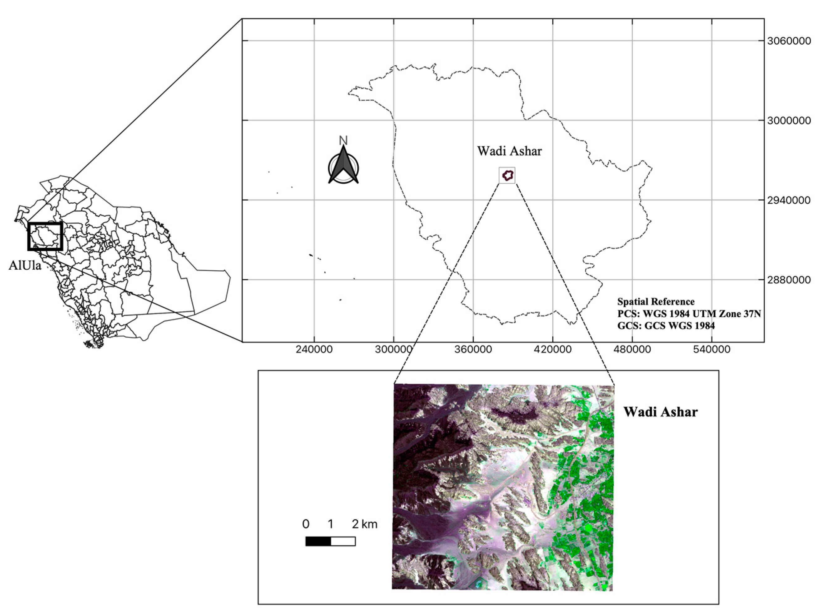
Figure 3.
Workflow for extracting principal spectral information from Sentinel-2 image dense time series.
Figure 3.
Workflow for extracting principal spectral information from Sentinel-2 image dense time series.
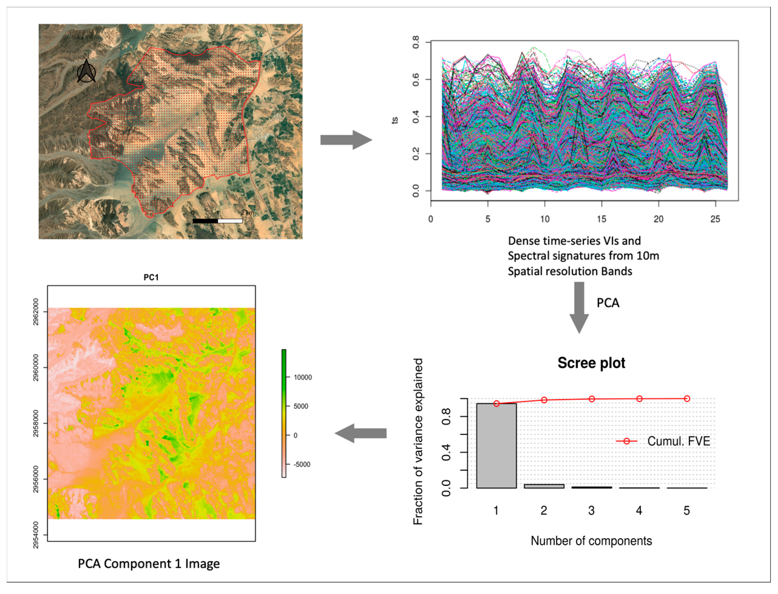
Figure 4.
Spatial consideration and estimation of unknown space for map predictions within area of applicability (AOA) of classification model. The top left panel shows predictions for known and unknown environmental space. Dissimilarity index (DI) estimated and mapped (top middle panel) as measurement threshold for unknown environmental space. The DI used as basis for model prediction within AOA (map at top right panel) – DI above the AOA threshold (bottom panel) is mapped out as outside AOA (unclassified areas).
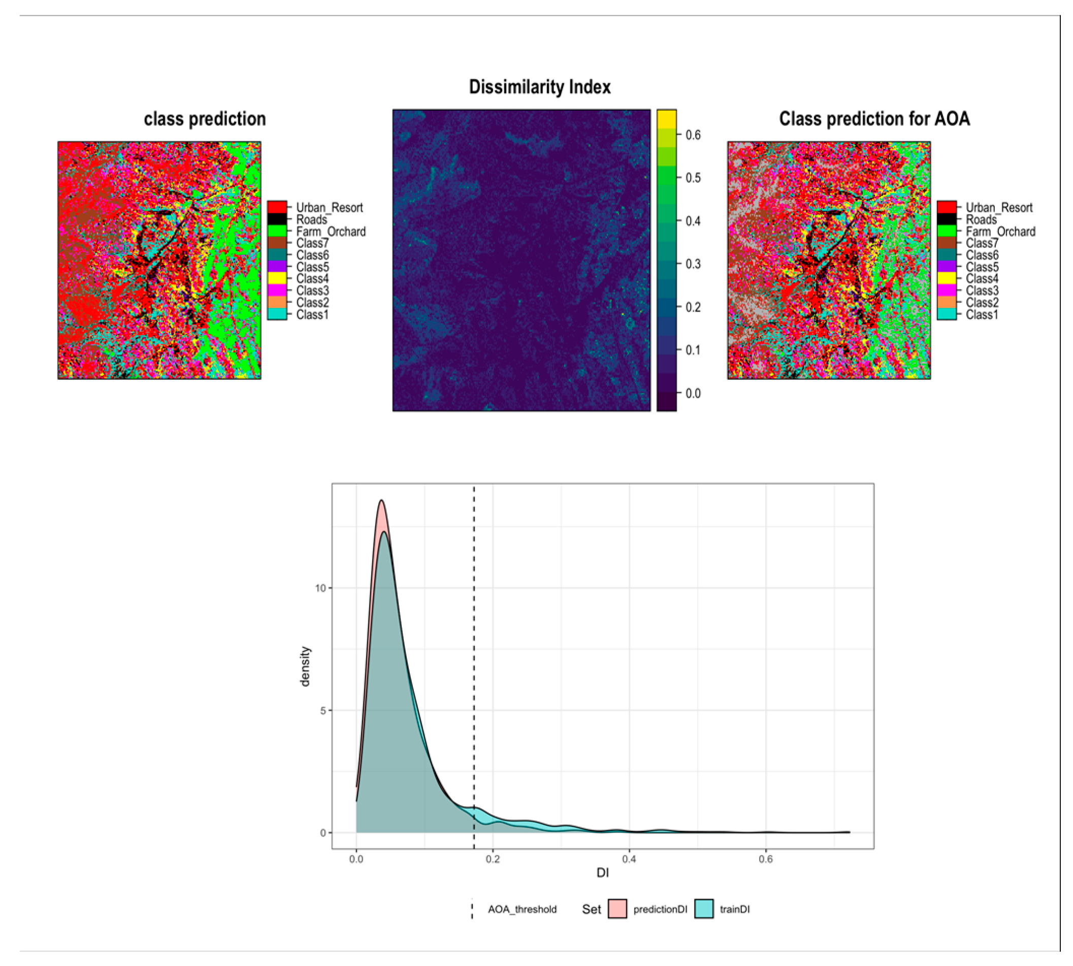
Figure 5.
Thematic maps of plant assemblages land cover categories based on the three classification models (top row) and the class (pixel) proportions in the respective maps (bottom row). Contrary to the other vegetation and land cover categories, the class-specific accuracy for farms and orchards (FO) did not vary as much with choice of spatial predictors. Our results highlight that the VIs-based classification, with comparably high overall accuracy (Kappa of 65.91%), had high variability in class-specific prediction probability. Vegetation assemblages with low height and density showed inconsistency in reliable (low uncertainty) prediction across the classification models. This uncertain accuracy reflects temporal and spatial variability in combination of vegetation structural and phenological traits. In desert landscapes, most vegetations have distinctive spatial patterns - their type and mechanism of formation are modulated by geomorphic processes amongst other landscape processes [67]. Most of the vegetation communities are a mixture of different species, with often different growth forms, providing different functions. Thus, distinctive plant assemblages often inhabit different niches distributed across micro-habitats in a landscape. The high uncertainty and quantity disagreement observed for vegetation index-based classification model is indicative of typical vegetation structural and forms that superpose variability in vegetation index. In an arid landscape in Africa, [30] observed that spatial and temporal variations in species dominance is likely a noise contributor in modelling relationship between NDVI and biomass.
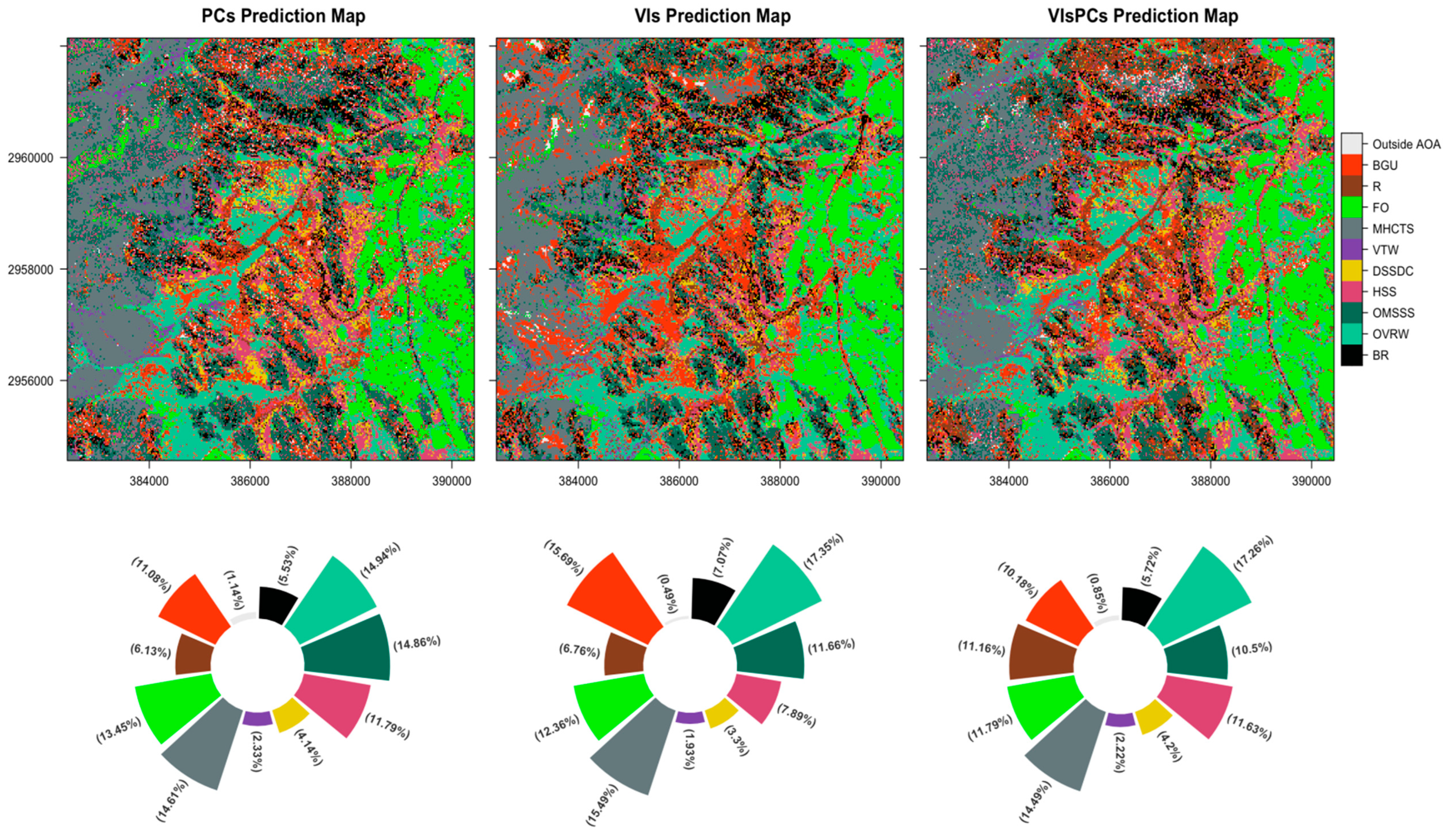
Figure 6.
Distribution of information uncertainty (Shannon Entropy) based on non-parametric probability (kernel) distribution estimates (top row) and the boxplot and non-parametric mean comparison of uncertainty (bottom row) for the predicted vegetation assemblages and land cover. Categories with significantly different mean entropy are indicated with an Asterix.
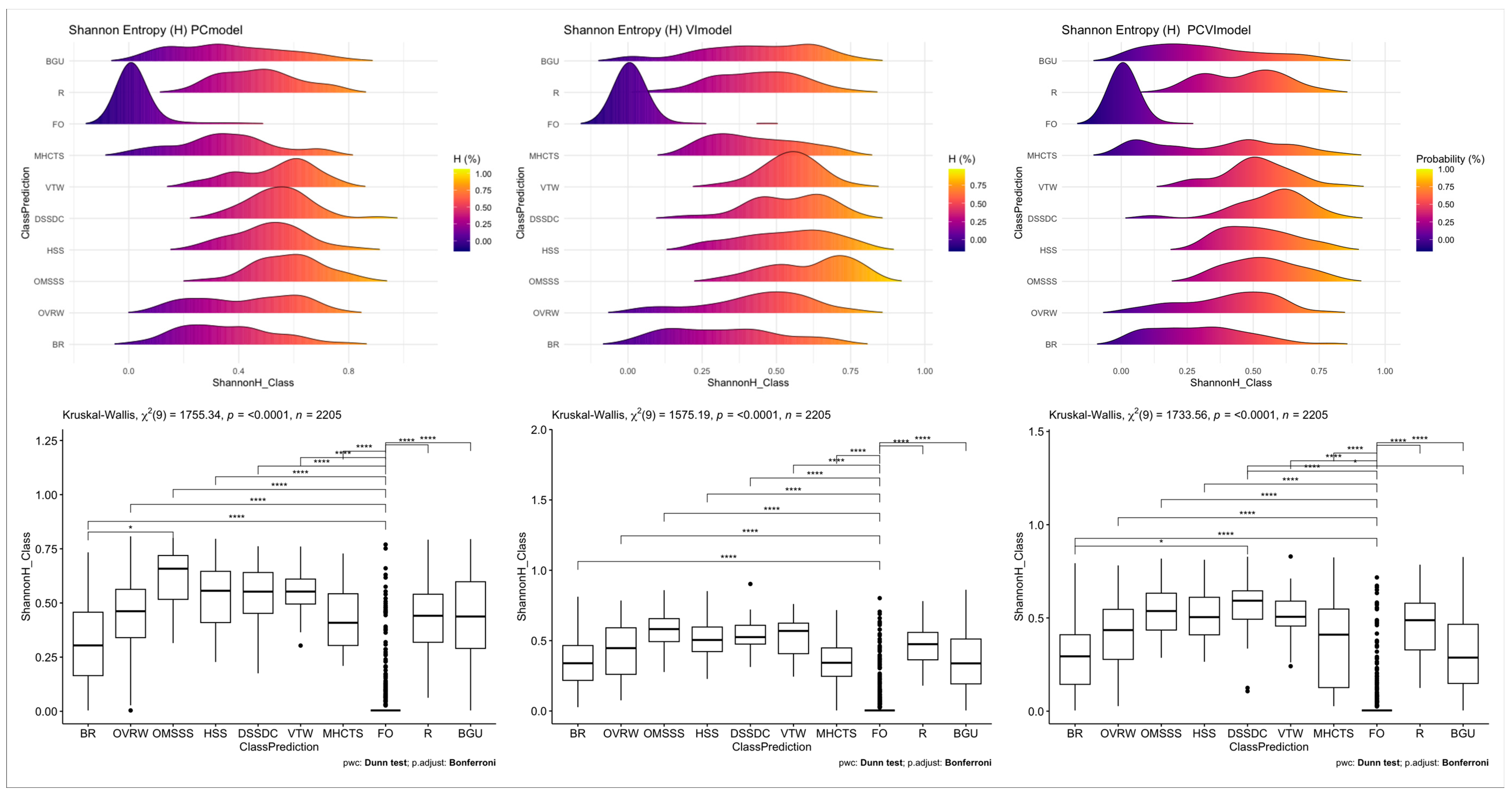
Figure 7.
Overall difference in class prediction between maps, as estimated by disagreements in class quantity and the spatial allocation or configuration (exchange and shift).
Figure 7.
Overall difference in class prediction between maps, as estimated by disagreements in class quantity and the spatial allocation or configuration (exchange and shift).
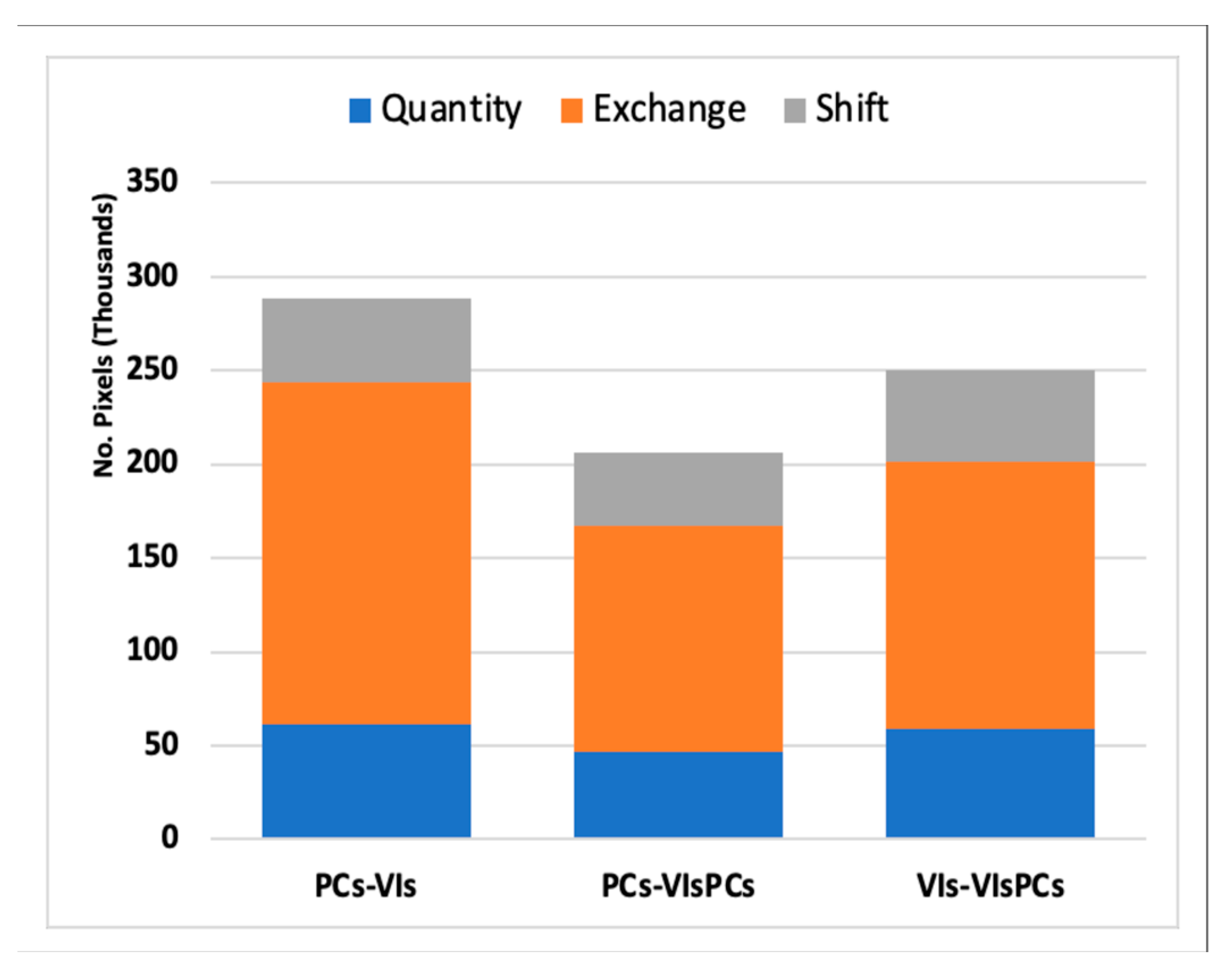
Figure 8.
Land cover/use category-level change intensity and class disagreement for the three predicted maps: (A) Graphs on the left show change intensity - the mapped categories are indicated as pair of bars - for loss and gain between the map intervals. Bars that extend to the left of 0 axis are the sizes (no. of pixels) of loss or gain, and those that extend to the right are the intensities (proportions) of loss Lti or gain Gtj – each the size of the corresponding bar to the left of 0 line divided by the category’s total size. For each map interval, the black dashed line represents the value of uniform spatial intensity St. If a bar extends above the uniform intensity line, the change intensity for the category is active. If a bar stops below the uniform intensity line, then the category is dormant; (B) Graphs show the three different class disagreements for the transition-level change intensity between each reference and comparison map. Labels for each category indicate the overall quantity difference between maps (Gain is the sum of pixels at reference or final map minus persistence, while Loss is the sum at comparison or initial map minus persistence).
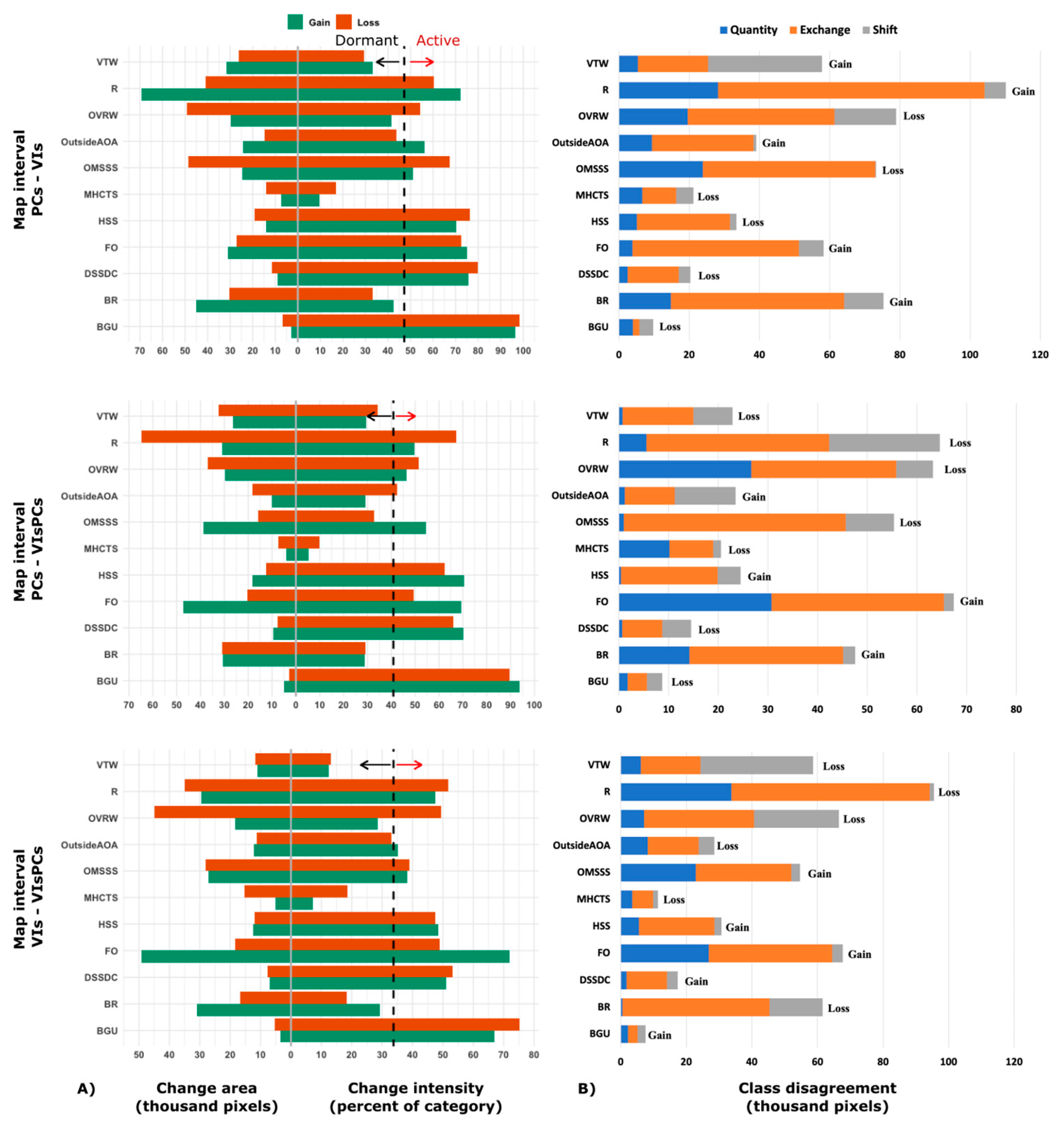
Figure 9.
Thematic map of plant assemblage distribution for the study area. The pictures illustrate some main vegetation assemblages observed during field surveys.
Figure 9.
Thematic map of plant assemblage distribution for the study area. The pictures illustrate some main vegetation assemblages observed during field surveys.
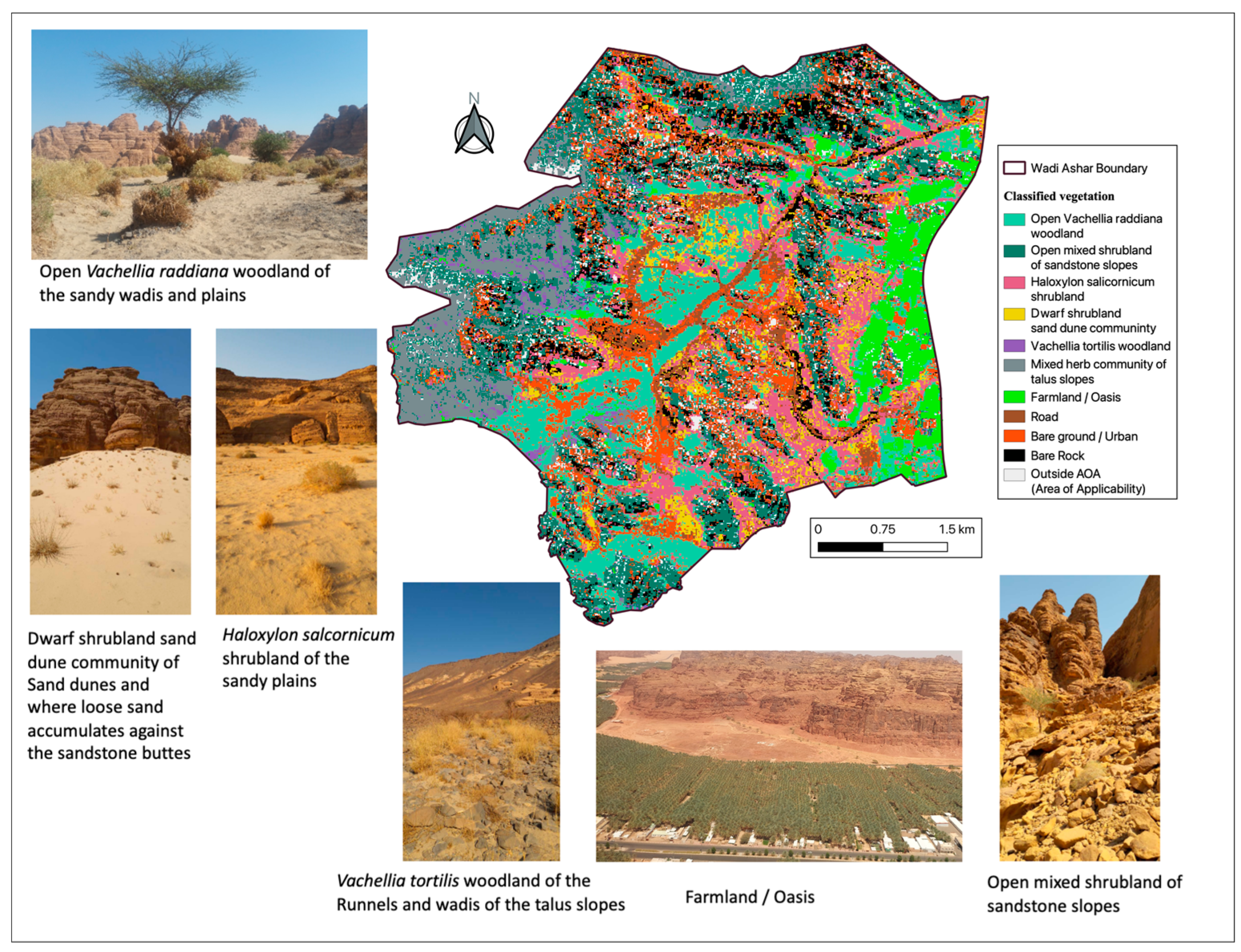

Table 1.
Summary of references pixels and areas (m2) for the vegetation and land cover classes.
| Vegetation and Land Cover Classes | No. Ref. Polygons | No. Ref. Pixels (10 × 10 m2) | Total Ref. Area (m2) |
| Class 1 - Open Vachellia raddiana Woodland (OVRW) | 38 | 121 | 11748.3 |
| Class 2 – Bare rock (BR) | 5 | 99 | 9762.1 |
| Class 3 - Open mixed shrubland of sandstone slopes (OMSSS) | 14 | 45 | 4328.3 |
| Class 4 - Haloxylon salicornicum shrubland (HSS) | 20 | 63 | 6183.3 |
| Class 5 - Dwarf shrubland sand dune community (DSSDC) | 16 | 49 | 4946.7 |
| Class 6 - Vachellia tortilis woodland (VTW) | 11 | 36 | 3400.8 |
| Class 7 - Mixed herb community of the talus slopes (MHCTS) | 12 | 37 | 3709.9 |
| Farms / Orchards (FO) | 84 | 1441 | 153520.5 |
| Roads (R) | 60 | 114 | 4637.5 |
| Bare ground / Urban (BGU) | 106 | 200 | 1310.9 |
Table 2.
Explained variance by 5 Principal Components (PCs) of PCA on the 20 Spectral bands.
| PC Layer | Explained Variance (%) | Cumulative Variance (%) |
| PC1 | 87.17 | 87.17 |
| PC2 | 7.64 | 94.81 |
| PC3 | 2.53 | 97.35 |
| PC4 | 1.33 | 98.67 |
| PC5 | 0.57 | 99.25 |
| Symbol | Meaning |
| i | index for a category at interval’s initial time point |
| j | index for a category at interval’s final time point |
| J | number of categories i.e. eleven for this study |
| t | index for time point |
| T | number of time points |
| Mt | map at time point t |
| Ctij | number of pixels that are category i at Mt and category j at Mt+1 i.e. total number of pixels that transition from category i to j. |
| Gtj | intensity of gain of category j during map interval [Mt, Mt+1] relative to size of category j at Mt+1 |
| Lti | intensity of loss of category i during map interval [Mt, Mt+1] relative to size of category i at Mt |
| Wtj | uniform intensity of transition from all non-j categories to category j during interval [Mt, Mt+1] relative to size of all non-j categories at Mt |
| Rtij | intensity of transition from category i to category j during interval [Mt, Mt+1] relative to size of category i at Mt |
| St | total change percentage during the interval [Mt, Mt+1] |
Table 4.
Illustration of confusion matrix and relationship between estimated intensity components.
| Categories in Map Mt+1 | |||||||
| j=1 | j=2 | j=3 | …… | j=J | LossIntensities | ||
| Categories in Map Mt | i=1 | Rt11 | Rt12 | Rt13 | …… | Rt1J | Lt1 |
| i=2 | Rt21 | Rt22 | Rt23 | …… | Rt2J | Lt2 | |
| i=3 | Rt31 | Rt32 | Rt33 | Rt3J | Lt3 | ||
| …… | ….. | ….. | ….. | …… | …… | ….. | |
| i=J | RtJ1 | RtJ2 | RtJ3 | …… | RtJJ | LtJ | |
| Uniform Transition Intensities | Wt1 | Wt2 | Wt3 | …… | WtJ | ||
| GainIntensities | Gt1 | Gt2 | Gt3 | …… | GtJ | ||
| All categories during interval [Mt, Mt+1] | St | ||||||
Table 5.
Summary statistics of the RF classification models from different predictor variables.
| PCs Model | VIs Model | VIsPCs Model | |
| Independent Variables | 5 | 5 | 10 |
| Selected Predictors | 5 | 4 | 5 |
| Overall Accuracy (OA) % (95% CI) | 80.32 (78.60, 81.96) | 80.68 (79.97, 82.31) | 82.71 (81.08, 84.28) |
| Kappa % | 65.42 | 65.91 | 69.51 |
| DI Threshold for AOA | 0.261 | 0.076 | 0.172 |
DI: Dissimilarity Index, AOA: Area of Applicability.
Table 6.
Plant assemblage (vegetation) classification model statistics.
| Class Prediction statistics | |||
| Models and Classes | F1-Score | Sensitivity | Specificity |
| PCs Model | |||
| BR | 0.7162 | 0.7777 | 0.9814 |
| OVRW | 0.6141 | 0.6446 | 0.9736 |
| OMSSS | 0.3917 | 0.4222 | 0.9847 |
| HSS | 0.3939 | 0.4127 | 0.9799 |
| DSSDC | 0.2278 | 0.1836 | 0.9902 |
| VTW | 0.0638 | 0.0833 | 0.9746 |
| MHCTS | 0.6133 | 0.6216 | 0.9930 |
| FO | 0.9632 | 0.9452 | 0.9673 |
| R | 0.3184 | 0.2807 | 0.9737 |
| BGU | 0.6529 | 0.7100 | 0.9536 |
| VIs Model | |||
| BR | 0.6698 | 0.7071 | 0.9810 |
| OVRW | 0.5395 | 0.6198 | 0.9606 |
| OMSSS | 0.2268 | 0.2444 | 0.9810 |
| HSS | 0.3275 | 0.3016 | 0.9841 |
| DSSDC | 0.3703 | 0.3061 | 0.9921 |
| VTW | 0.2195 | 0.2500 | 0.9829 |
| MHCTS | 0.6000 | 0.5675 | 0.9944 |
| FO | 0.9711 | 0.9556 | 0.9764 |
| R | 0.4279 | 0.4035 | 0.9737 |
| BGU | 0.6385 | 0.6800 | 0.9551 |
| VIsPCs Model | |||
| BR | 0.7336 | 0.7374 | 0.9872 |
| OVRW | 0.5631 | 0.7190 | 0.9515 |
| OMSSS | 0.4634 | 0.4222 | 0.9917 |
| HSS | 0.4000 | 0.4444 | 0.9771 |
| DSSDC | 0.2272 | 0.2041 | 0.9865 |
| VTW | 0.3529 | 0.3333 | 0.9908 |
| MHCTS | 0.6865 | 0.6216 | 0.9968 |
| FO | 0.9732 | 0.9577 | 0.9804 |
| R | 0.4205 | 0.3947 | 0.9737 |
| BGU | 0.7223 | 0.7350 | 0.9701 |
Disclaimer/Publisher’s Note: The statements, opinions and data contained in all publications are solely those of the individual author(s) and contributor(s) and not of MDPI and/or the editor(s). MDPI and/or the editor(s) disclaim responsibility for any injury to people or property resulting from any ideas, methods, instructions or products referred to in the content. |
© 2025 by the authors. Licensee MDPI, Basel, Switzerland. This article is an open access article distributed under the terms and conditions of the Creative Commons Attribution (CC BY) license (http://creativecommons.org/licenses/by/4.0/).
Copyright: This open access article is published under a Creative Commons CC BY 4.0 license, which permit the free download, distribution, and reuse, provided that the author and preprint are cited in any reuse.


