Assessing the Dimensionality Reduction of the Geospatial Dataset Using Principal Component Analysis (PCA) and Its Impact on the Accuracy and Performance of Ensembled and Non-ensembled Algorithms

Farkhanda Abbas; Feng Zhang; Javed Iqbal; Fazila Abbas; Abdulwahed Fahad Alrefaei; Mohammed Albeshr

doi:10.20944/preprints202307.0529.v1

Submitted:

07 July 2023

Posted:

10 July 2023

You are already at the latest version

Abstract

In this study, our primary objective was to analyze the tradeoff between accuracy and complexity in machine learning models, with a specific focus on the impact of reducing complexity and entropy on the production of landslide susceptibility maps. We aimed to investigate how simplifying the model and reducing entropy can affect the capture of complex patterns in the susceptibility maps. To achieve this, we conducted a comprehensive evaluation of various machine-learning algorithms for classification tasks. We compared the performance of these algorithms in terms of accuracy and complexity, considering both "before" and "after" scenarios of dimensionality reduction using Principal Component Analysis (PCA). Our findings revealed that reducing complexity and lowering entropy can lead to an increase in model accuracy. However, we also observed that this reduction in complexity comes at the cost of losing important complex patterns in the produced landslide susceptibility maps. By simplifying the model and reducing entropy, certain intricate relationships and uncertain patterns may be overlooked, resulting in a loss of information and potentially compromising the accuracy of the susceptibility maps. The analysis encompassed a diverse range of machine learning algorithms, including Random Forest (RF), Extra Trees (EXT), XGboost, LightGBM, Catboost, Naive Bayes (NB), K-Nearest Neighbors (KNN), Gradient Boosting Machine (GBM), and Decision Trees (DT). Each algorithm was evaluated for its strengths and limitations, considering the tradeoff between accuracy and complexity. Before dimensionality reduction, the algorithms demonstrated promising results, with RF exhibiting excellent AUC/ROC scores and average accuracy. However, computational costs were noted as a potential drawback for RF, especially when dealing with large datasets. EXT showcased robust performance and good accuracy, while XGboost demonstrated its ability to handle complex relationships within large datasets, albeit requiring careful hyperparameter tuning. The efficiency and scalability of LightGBM made it a suitable choice for large datasets, although it displayed sensitivity to class imbalance. Catboost excelled in handling categorical features, but longer training times were observed for larger datasets. NB showcased simplicity and computational efficiency but assumed independence among features. KNN, known for its capability to capture local patterns and spatial relationships, was found to be sensitive to the choice of distance metric. GBM, while capturing complex relationships effectively, was prone to overfitting without proper regularization. DT, with its interpretability and ease of understanding, faced limitations in terms of overfitting and limited generalization. After dimensionality reduction, certain algorithms exhibited improvements in their AUC/ROC scores and average accuracy, including RF, EXT, XGboost, and LightGBM. However, for a few algorithms, such as NB and DT, a decrease in performance was observed. This study provides valuable insights into the performance characteristics, strengths, and limitations of various machine learning algorithms in classification tasks. Researchers and practitioners can utilize these findings to make informed decisions when selecting algorithms for their specific datasets and requirements. We also aim to identify the potential factors contributing to the high accuracy rates obtained from these ensembled algorithms and explore possible shortcomings of non-ensembled algorithms that may result in lower accuracy rates. By conducting a comprehensive analysis of these algorithms, we seek to provide valuable insights into the benefits and limitations of ensembled approaches for landslide susceptibility mapping. Our study sheds light on the challenges faced when balancing accuracy and complexity in machine learning models for landslide susceptibility mapping. It emphasizes the importance of carefully considering the level of complexity and entropy reduction in relation to the specific patterns and uncertainties present in the data. By providing insights into this tradeoff, our research aims to assist researchers and practitioners in making informed decisions regarding model complexity and entropy reduction, ultimately improving the quality and interpretability of landslide susceptibility maps.

Keywords:

machine learning

;

accuracy

;

complexity

;

entropy

;

landslide susceptibility mapping

;

dimensionality reduction

;

Principal Component Analysis (PCA)

Subject:

Computer Science and Mathematics - Artificial Intelligence and Machine Learning

Introduction

Landslides pose significant threats to human life, infrastructure, and the environment, making landslide susceptibility mapping a crucial task in assessing and mitigating these risks. Accurate identification of areas prone to landslides allows for proactive planning and effective implementation of measures to minimize potential damages. Machine learning algorithms have proven to be valuable tools in landslide susceptibility mapping due to their ability to analyze complex spatial relationships and patterns. Ensemble learning, a powerful approach that combines multiple models to make collective predictions, has gained prominence in various fields of machine learning. In this research paper, we investigate the effectiveness of ensemble algorithms, with a particular focus on gradient boosting algorithms such as GBM, LightGBM, and Catboost, in the context of landslide susceptibility mapping. These algorithms have demonstrated superior performance in diverse applications and are known for their ability to handle large datasets and capture intricate nonlinear relationships [1,2,3]. Furthermore, we compare the results of gradient boosting algorithms with other ensemble methods, specifically Random Forest (RF) and Extra Trees (EXT), which also belong to the ensemble family. Additionally, we explore the performance of non-ensemble machine learning algorithms, including Decision Tree (DT), K-Nearest Neighbors (KNN), and Naive Bayes (NB), which serve as representatives of standalone algorithms from different paradigms.

The concept of entropy is often misunderstood in the scientific community [4,5], and there are speculations suggesting that reducing entropy automatically reduces the complexity of a model and improves accuracy. However, this assumption does not hold true in real-world scenarios, particularly when dealing with complex phenomena like landslides. In fact, when using reduced dimensionality datasets generated through techniques like PCA, important patterns may be lost, leading to incomplete maps that fail to capture crucial information obtained from more complex and variable datasets that is evident from the maps obtained through modified geospatial dataset with low dimensionality see Figure 6. Therefore, it is imperative to develop advanced methods that can effectively encompass the uncertainty and complex dynamics inherent in real-life scenarios, such as landslides. These methods should go beyond simplistic approaches that aim to reduce complexity and instead focus on accurately representing the complex nature of land sliding. To achieve this, it is crucial to explore sophisticated techniques that can handle uncertainty and complex effects. Ensemble modeling, for instance, combines multiple models to account for variability and capture different aspects of the intricate landslide processes. By leveraging the strengths of various models, ensemble techniques can address the limitations of individual models and provide more robust and accurate predictions. Furthermore, incorporating advanced modeling approaches like machine learning algorithms, geostatistics, or hybrid models that integrate multiple data sources and consider spatial dependencies can enhance the accuracy of landslide susceptibility mapping. These techniques enable us to better understand and simulate the complexities and uncertainties associated with landslides.

In summary, the misguided notion that reducing entropy automatically improves accuracy by simplifying models is not applicable to complex phenomena like landslides verified from Figure 6. Instead, it is crucial to develop advanced methods that can effectively incorporate uncertainty and complex dynamics into our models. By adopting these sophisticated approaches, we can more accurately simulate and predict real-life complex scenarios, such as land sliding, ultimately leading to improved risk assessment and management strategies [4,6,7,8,9].

Principal Component Analysis (PCA) is a commonly used method for reducing the dimensionality of datasets. In our experiment, we employed PCA to reduce the dimensionality of the geospatial dataset. PCA is a technique that aims to transform a high-dimensional dataset into a lower-dimensional space while preserving the most significant information. It achieves this by identifying the principal components, which are orthogonal directions that capture the maximum variance in the data. By selecting a subset of the principal components, you can effectively reduce the dimensionality of the dataset. In the context of our study on landslide susceptibility mapping, we use PCA to reduce the dimensionality of the geospatial dataset to analyze the impact reducing dimensionality by removing the variable with high variability in order to obtain a simple less complex geospatial dataset so that we can effective identify the impact of dimensionality reduction on geospatial dataset and susceptibility maps produce by dataset with reduce dimensionality [10,11,12,13,14].

The primary objective of this study is to evaluate the performance of various ensembled and non-ensembled algorithms for landslide susceptibility mapping. The study aims to reduce the entropy of a geospatial dataset and examine the impact of entropy reduction on the accuracy of the mentioned algorithms. Additionally, the study seeks to gain insights into the factors contributing to the high accuracy rates observed in ensembled algorithms and identify potential shortcomings of non-ensembled algorithms that may result in lower accuracy rates. To achieve these goals, a comprehensive experimental setup is employed. A carefully curated dataset is utilized, consisting of relevant geospatial and environmental features, which will be used to train and validate the selected algorithms. The geospatial dataset is modified using Principal Component Analysis (PCA) to reduce its complexity. The modified dataset obtained from PCA is then used to run both ensembled and non-ensembled algorithms. Performance metrics are employed to assess and compare the accuracy of each algorithm's landslide susceptibility predictions before and after dimensionality reduction. By comparing the performance of the algorithms on the original and reduced datasets, the study aims to determine the impact of dimensionality reduction on the overall accuracy of susceptibility maps and the accuracy of the algorithms themselves.

The study intends to provide valuable insights into the reasons behind the high accuracy rates observed in ensembled algorithms compared to non-ensembled algorithms. It also aims to identify potential shortcomings of non-ensembled algorithms that may lead to lower accuracy rates. By analyzing the effect of dimensionality reduction on the accuracy of susceptibility maps and algorithms, the study aims to highlight the importance of data preprocessing techniques for improving the performance of landslide susceptibility mapping models. In summary, the study focuses on assessing the performance of ensembled and non-ensembled algorithms for landslide susceptibility mapping, analyzing the impact of entropy reduction on accuracy, and evaluating the effect of dimensionality reduction on both susceptibility maps and algorithm accuracy. The results of this study can contribute to improving landslide risk assessment and management strategies. The findings of this research paper contribute to the growing body of knowledge in landslide susceptibility mapping and provide valuable insights for decision-makers and researchers in the field. Understanding the strengths and weaknesses of ensembled algorithms compared to non-ensembled algorithms can guide the selection and implementation of appropriate techniques for accurate and reliable landslide susceptibility mapping. In this research paper, the we aimed to compare and analyze the performance of different algorithms for landslide susceptibility mapping. The algorithms evaluated in the study include Random Forest (RF), Extra Trees (EXT), XGboost, LightGBM, Catboost, Naive Bayes (NB), K-Nearest Neighbors (KNN), Gradient Boosting Machine (GBM), and Decision Tree (DT). The evaluation was based on the AUC/ROC score and average accuracy as performance metrics. Based on the results presented in the paper, the ensemble algorithms (RF, EXT, XGboost, LightGBM, Catboost, and GBM) generally achieved higher AUC/ROC scores and average accuracies compared to the non-ensemble algorithms (NB, KNN, and DT) [15,16,17] . This indicates that the ensemble algorithms, which combine multiple models, were more effective in capturing the complexities of landslide susceptibility mapping. Among the ensemble algorithms, RF obtained the highest AUC/ROC score of 0.96497, indicating its strong predictive capability. EXT, XGboost, LightGBM, and Catboost also performed well with AUC/ROC scores ranging from 0.95893 to 0.96316. These algorithms consistently outperformed the non-ensemble algorithms in terms of both AUC/ROC score and average accuracy. On the other hand, the non-ensemble algorithms (NB, KNN, and DT) achieved relatively lower AUC/ROC scores and average accuracies. NB had the highest AUC/ROC score among the non-ensemble algorithms with 0.95410, followed by KNN with 0.84782, and DT with 0.83454. These results suggest that the non-ensemble algorithms may struggle to capture the intricate relationships between the features and landslide susceptibility accurately.

Based on the AUC/ROC scores, the Random Forest algorithm (RF) achieves the highest score of 0.96497, followed closely by CatBoost with a score of 0.96316. These two algorithms outperform the others in terms of their ability to distinguish between positive and negative classes.

Regarding average accuracy, Random Forest (RF) also achieves the highest accuracy of 0.92020, followed by CatBoost with an accuracy of 0.91417. These algorithms perform better on average across the evaluation samples. It's important to note that the performance of an algorithm may vary depending on the specific task and dataset. Therefore, it's recommended to consider other factors such as computational efficiency, interpretability, and scalability when selecting an algorithm for a particular application.

One possible reason why CatBoost performed similarly to Random Forest (RF) could be because both algorithms are ensemble methods that are designed to handle complex datasets and capture non-linear relationships. Both CatBoost and Random Forest have the ability to handle categorical features effectively. CatBoost incorporates a gradient boosting framework specifically designed to handle categorical variables by using a combination of ordered boosting and symmetric trees. Random Forest, on the other hand, builds an ensemble of decision trees and can handle categorical variables through techniques such as one-hot encoding or binary encoding.

Additionally, both algorithms have a high capacity for capturing interactions and non-linear relationships in the data, which can contribute to their similar performance. They both excel in handling high-dimensional datasets and are robust to outliers and noise. It's important to note that while CatBoost and Random Forest achieved similar results in terms of AUC/ROC scores and average accuracy, they may have different strengths and weaknesses in other aspects such as computational efficiency, interpretability, or sensitivity to hyperparameters. It would be worthwhile to further analyze and compare these factors to make a more comprehensive assessment of their performance for a specific task or dataset.

Ensemble algorithms outperformed non-ensemble algorithms: The ensemble algorithms, including RF, EXT, XGboost, LightGBM, Catboost, and GBM, consistently achieved higher AUC/ROC scores and average accuracies compared to the non-ensemble algorithms (NB, KNN, and DT). This pattern highlights the effectiveness of ensemble methods in improving the accuracy of landslide susceptibility mapping. RF demonstrated the highest performance: Among the algorithms evaluated, RF exhibited the highest AUC/ROC score of 0.97524, indicating its superior predictive capability for landslide susceptibility mapping. This suggests that RF may be particularly suitable for accurately identifying landslide-prone areas [18,19,20]. Gradient boosting algorithms performed consistently well: XGboost, LightGBM, and GBM achieved similar AUC/ROC scores and average accuracies, indicating their comparable performance in landslide susceptibility mapping. This suggests that gradient boosting algorithms can be reliable choices for accurate prediction in this context [21,22,23,24]. Non-ensemble algorithms had lower performance. The non-ensemble algorithms, including NB, KNN, and DT, generally obtained lower AUC/ROC scores and average accuracies compared to the ensemble algorithms [25,26,27]. This suggests that standalone algorithms may struggle to capture the complex relationships and patterns associated with landslide susceptibility effectively. Overall, the paper demonstrates that ensemble algorithms, particularly RF and gradient boosting algorithms, are well-suited for landslide susceptibility mapping, providing high accuracy and reliable predictions before and after dimensionality reduction. The findings highlight the importance of considering ensemble methods when developing models for landslide risk assessment and mitigation.

The primary objectives of this research paper are as follows:

Evaluate the performance of gradient boosting algorithms, including GBM, LightGBM, and Catboost, for landslide susceptibility mapping. Analyze the differences in the implementation and optimization strategies of these gradient boosting algorithms. Assess the accuracy rates and predictive capabilities of these algorithms in identifying landslide-prone areas before and after dimensionality reduction of geospatial dataset.
Compare the performance of ensemble methods, specifically Random Forest (RF) and Extra Trees (EXT), with gradient boosting algorithms for landslide susceptibility mapping. Investigate the strengths and weaknesses of each ensemble method in capturing complex spatial relationships and patterns related to landslides. Determine the effectiveness of ensemble methods in improving accuracy compared to standalone gradient boosting algorithms.
Evaluate the performance of non-ensembled machine learning algorithms, including Decision Tree (DT), K-Nearest Neighbors (KNN), and Naive Bayes (NB), for landslide susceptibility mapping. Assess the accuracy rates and limitations of these non-ensembled algorithms in capturing the complexities of landslide-prone areas. Identify potential challenges and shortcomings of non-ensembled algorithms that may lead to lower accuracy rates.
Identify the factors contributing to the high accuracy rates obtained from the ensembled algorithms and explore possible problems with non-ensembled algorithms that might lead to lower accuracy rates. Investigate the impact of dataset characteristics, feature selection, and algorithmic approaches on the performance of ensembled and non-ensembled algorithms. Gain insights into the reasons behind the superior performance of ensembled algorithms and potential limitations of non-ensembled algorithms.
Provide valuable insights and recommendations for selecting appropriate algorithms for accurate and reliable landslide susceptibility mapping. Compare the strengths and weaknesses of ensemble algorithms and non-ensemble algorithms in the context of landslide susceptibility mapping. Discuss the implications of the findings for decision-makers, researchers, and practitioners involved in landslide risk assessment and mitigation.
Provide a balance approach to handle complexity and accuracy together to efficiently represent the uncertainty in complex phenomena like land sliding.

By achieving these objectives, this research paper aims to contribute to the understanding of the performance and effectiveness of ensembled and non-ensembled algorithms for landslide susceptibility mapping. The insights gained from this study can facilitate informed decision-making and help improve the accuracy and reliability of landslide risk assessment and mitigation strategies.

In the following sections, we discuss the methodology, including the description of the dataset, the ensembled algorithms employed, and the non-ensembled algorithms selected and describe the modified geospatial dataset created using PCA with reduce dimensionality. We then present the experimental setup, the obtained results, and subsequent discussions. Finally, we conclude the paper by summarizing the key findings, discussing their implications, and obtained results before and after reduction of complexity of geospatial dataset.

Background

Landslides are natural hazards that result from the downward movement of rocks, soil, and debris on sloping terrains. They are triggered by various factors, including heavy rainfall, seismic activity, slope instability, and human-induced activities. Landslides have severe consequences, leading to loss of life, destruction of infrastructure, and ecological damage. Therefore, accurately assessing landslide susceptibility is crucial for effective land management, urban planning, and disaster risk reduction. Traditionally, landslide susceptibility mapping relied on expert knowledge, geological surveys, and field observations. However, these methods often lacked objectivity and struggled to handle the complex relationships and spatial patterns associated with landslides. With the advancement of machine learning techniques and the availability of geospatial data, automated approaches have gained prominence in landslide susceptibility mapping. Machine learning algorithms offer the ability to analyze large volumes of geospatial data and identify complex patterns and relationships that are difficult to capture using conventional methods. These algorithms learn from historical landslide occurrences and associated factors to generate predictive models. By considering various environmental, geological, and topographical features, machine learning models can accurately assess the susceptibility of an area to landslides [28,29,30,31].

Ensemble learning has emerged as a powerful approach in machine learning, particularly for complex prediction tasks. Ensemble algorithms combine multiple models to make collective predictions, leveraging the strengths of individual models and reducing the impact of their weaknesses. This approach has been successful in improving accuracy and robustness in various domains, including image recognition, natural language processing, and data mining.

Gradient boosting algorithms, such as GBM (Gradient Boosting Machine), LightGBM, and Catboost, have become popular choices for ensemble learning tasks . These algorithms construct a series of weak learners (decision trees) sequentially, with each subsequent learner focusing on the errors made by the previous ones. By iteratively minimizing the prediction errors, gradient boosting algorithms produce highly accurate models that can effectively handle complex relationships in the data [21,32,33]. In addition to ensemble methods, non-ensembled machine learning algorithms have also been employed for landslide susceptibility mapping. Decision Tree (DT) is a standalone decision-based algorithm that constructs a tree-like model, making decisions based on feature values. K-Nearest Neighbors (KNN) is a distance-based algorithm that classifies samples based on the proximity to their neighboring instances. Naive Bayes (NB) is a probabilistic classifier that assumes independence between features. While previous studies have explored the application of both ensembled and non-ensembled algorithms in landslide susceptibility mapping, a comprehensive comparison and analysis of their performance and the factors contributing to their accuracy rates are still needed. This research paper aims to bridge this gap by conducting a systematic investigation of various ensembled algorithms, including gradient boosting methods, as well as non-ensembled algorithms for landslide susceptibility mapping. By evaluating their performance and identifying their strengths and weaknesses, we can provide valuable insights for improving landslide risk assessment and mitigation strategies.

Entropy is a concept originating from information theory that quantifies the uncertainty or randomness in a dataset. In the context of machine learning and data analysis, entropy measures the impurity or disorder of a set of samples with respect to their class labels. In the context of capturing complex phenomena, entropy plays a crucial role. High entropy indicates a higher degree of uncertainty or complexity in the dataset. It suggests that the dataset contains diverse patterns, variations, and uncertain relationships between variables. By capturing and incorporating this complexity through high entropy, machine learning models can better represent and understand the underlying intricate relationships and patterns within the data. High entropy enables the model to capture the nuances and uncertainties inherent in complex phenomena. It allows the model to flexibly adapt to the diverse patterns present in the data, thereby enhancing its ability to generalize and make accurate predictions or classifications. By considering the full range of possibilities and variations reflected in high entropy, the model becomes more robust and capable of handling complex, real-world scenarios. However, it is important to note that there is a tradeoff between complexity and model interpretability. Very high entropy or complexity can make it challenging to understand and interpret the model's decision-making process. Therefore, finding the right balance between capturing complex patterns through high entropy and maintaining interpretability is a key consideration in model development and analysis. Thus entropy is important for capturing complex phenomena as it quantifies the uncertainty and diversity in the dataset. It enables machine learning models to adapt to the complex patterns and variations present in the data, improving their ability to make accurate predictions and classifications. Balancing entropy with model interpretability is crucial for gaining insights and understanding the underlying relationships within complex systems [34,35,36,37].

Entropy is highly important when it comes to land sliding because landslides are complex phenomena that involve various factors and uncertainties. Landslides can be influenced by geological characteristics, topography, soil properties, precipitation patterns, vegetation cover, and human activities, among other factors. By considering entropy in landslide analysis, we can capture the diversity and variability present in the dataset, which is crucial for understanding and predicting landslides. High entropy indicates a higher degree of complexity and uncertainty in the data, which aligns with the multifaceted nature of landslides. It allows machine learning models to capture the diverse patterns, interactions, and relationships between different variables involved in landslides. Including entropy in landslide analysis helps to account for the inherent uncertainties and variations associated with landslides can be observed by landslide susceptibility maps created with complex dataset before dimensionality reduction in Figure 5. It enables models to consider different combinations of factors and their potential influences on landslides. This can lead to more accurate landslide susceptibility mapping, hazard assessment, and early warning systems. Furthermore, landslides can exhibit spatial and temporal variations, making it essential to capture the complexity and uncertainty through entropy. High entropy helps to account for these variations and provides a more comprehensive understanding of landslides across different regions and time periods. Thus entropy is of significant importance in land sliding as it enables the consideration of complex relationships and uncertainties associated with landslides. By incorporating entropy in landslide analysis, we can improve our understanding, prediction, and management of landslides, ultimately contributing to effective landslide risk reduction and mitigation strategies [38,39,40].

Methodology

Obtain a comprehensive dataset consisting of geospatial and environmental features relevant to landslide susceptibility mapping. Include features such as slope gradient, elevation, land cover, geological characteristics, distance to road, distance to streams, distance to fault lines and past landslide occurrences. Ensure the dataset covers a diverse range of geographical locations and includes both landslide-prone and non-landslide-prone areas. We selected two different groups of machine learning algorithms ensembled and non-ensembled. And we also examine the effect of eliminating the principle component with highest variance ratio that is aspect in our case study and examine its effect on overall accuracy of ensembled and non-ensembled algorithms. For that purpose we remove the "Aspect" and “Fault” feature from our dataset that capture most of the variability, creating a modified dataset without this component. Optionally, you can perform any other necessary preprocessing steps, such as handling missing values, scaling the data, or encoding categorical variables etc. Split the modified dataset into training and testing sets to evaluate the performance of the algorithms. Select the ensembled algorithms you want to experiment with, such as Random Forest, Extra Trees, XGBoost, Gradient Boosting, or other non-ensembled such as such as Naive Bayes, K-Nearest Neighbors, Decision Tree. Train and evaluate the ensembled and non-ensembled algorithms using the modified dataset without the "Aspect" feature. Measure the accuracy and any other relevant evaluation metrics. Based on the results, we can assess the effect of eliminating the "Aspect" feature on the overall accuracy of the ensembled and non-ensembled algorithms. Draw conclusions about the importance of the "Aspect" and ‘’Fault”feature and its contribution to the accuracy of the algorithms. Consider potential implications, such as improvements in computational efficiency or changes in the models' interpretability.

The variable with the highest variance ratio represents the feature that contributes the most to the overall variability in the dataset. Removing it may result in a loss of significant information, potentially impacting the accuracy of the algorithms. The high variance ratio suggests that the variable contains valuable information that may be relevant for the prediction task but in this experiment our main objective is to reduce the dimensionality and complexity of our dataset. PCA is a dimensionality reduction technique that aims to capture the most important patterns and variability in the data using a smaller number of orthogonal principal components. The principal components are derived from linear combinations of the original features, and each component represents a different direction in the feature space. The variance ratio associated with each principal component indicates the proportion of total variance in the dataset that can be explained by that component. The component with the highest variance ratio captures the most significant variability in the data.

When we remove the principal component with the highest variance ratio, we are effectively discarding the information that it represents. This can lead to a reduction in the dimensionality of the dataset, as one less feature is considered for analysis. Removing a principal component with high variance ratio implies that it contributes less to the overall variability in the dataset result in reducing the complexity of the dataset.

However, it's important to note that removing a principal component is a trade-off between dimensionality reduction and the potential loss of information. The impact on the accuracy of subsequent analysis or modeling tasks should be carefully evaluated, as some important patterns or relationships captured by the removed component may be lost but our major aim in this experiment is find the impact of dimensionality and complexity reduction of geospatial data on accuracy and performance of ensembled and non-ensembled algorithms.

One of the main reasons for using PCA is to reduce the dimensionality of the dataset. By eliminating the principal component with the highest variance ratio, you are reducing the dimensionality by one. This can be beneficial in terms of computational efficiency, memory usage, and model interpretability. However, it is important to assess the impact on the overall accuracy of your algorithms.

Ensembled Algorithms:

Select gradient boosting algorithms, including GBM, LightGBM, and Catboost, as the primary focus of the study. Study and analyze the implementation and optimization strategies specific to each algorithm. Configure the hyperparameters of each algorithm, such as learning rate, number of trees, and tree depth, based on best practices and prior research. Include Random Forest (RF) and Extra Trees (EXT) as representative ensemble methods for comparison.

Non-Ensembled Algorithms:

Select Decision Tree (DT), K-Nearest Neighbors (KNN), and Naive Bayes (NB) as representative non-ensembled algorithms. Implement and configure these algorithms using appropriate settings and hyperparameters. Ensure that the decision tree depth, number of neighbors in KNN, and smoothing parameters in NB are appropriately determined.

Conduct exploratory data analysis to understand the distribution and characteristics of the dataset. Handle missing values, outliers, and inconsistencies in the dataset through appropriate preprocessing techniques. Perform feature engineering, such as scaling, normalization, and transformation, to ensure compatibility and improve algorithm performance. In this research, the dataset was split into training and validation subsets using a sampling strategy that involved allocating 70% of the data for training purposes and 30% for testing. Additionally, a 3-fold cross-validation technique was employed. This approach helps assess the model's performance by training and evaluating it on different subsets of the data.

Validate the trained models using the validation subset and evaluate their performance using appropriate metrics such as accuracy, precision, recall, and area under the receiver operating characteristic curve (AUC-ROC). Compare the performance of ensembled algorithms (gradient boosting, RF, and EXT) with non-ensembled algorithms (DT, KNN, and NB). Identify the factors contributing to the high accuracy rates of ensembled algorithms and explore potential challenges with non-ensembled algorithms. Discuss the implications of the findings, including the strengths and limitations of each algorithm, in the context of landslide susceptibility mapping. By following this methodology, the study aims to provide a comprehensive analysis and comparison of ensembled and non-ensembled algorithms for landslide susceptibility mapping. The approach ensures a fair evaluation of each algorithm's performance and facilitates the identification of key factors that contribute to their accuracy rates.

Dataset Description

The dataset used in this research paper comprises geospatial and environmental features relevant to landslide susceptibility mapping. The dataset is carefully curated to include a wide range of factors associated with landslide occurrences and covers diverse geographical locations. The following are the source and key features included in the dataset.

Table 1. source of dataset.

Data source	Input variables	Scale/Resolution	Source
Sentinel 2 satellite images	landslide inventory, LCLU, Road network	10m
DEM	Slope Aspect Stream Network	30 m	SRTM Shuttle Radar Topography Mission (USGS) United States Geological Survey
Geological Map	Geology Units and Fault lines	30 m	Geological Survey of Pakistan
Google Earth Maps	Landslide Inventory Land Cover/Land Use Road Network	2–5 m
Field Survey	GPS Points	1 m

Table 2. key features included in the dataset.

Factors	Classes	Class Percentage %	Landslide Percentage %	Reclassification
Slope (°)	Very Gentle Slope < 5°	17.36	21.11	Geometrical interval reclassification
	Gentle Slope 5°–15°	20.87	28.37
	Moderately Steep Slope 15°–30°	26.64	37.89
	Steep Slope 30°–45°	24.40	10.90
	Escarpments > 45°	10.71	1.73
Aspect	Flat (−1)	22.86	7.04	Remained unmodified (as in source data).
	North (0–22)	21.47	7.03
	Northeast (22–67)	14.85	5.00
	East (67–112)	8.00	11.86
	Southeast (112–157)	5.22	14.3
	South (157–202)	2.84	14.40
	Southwest (202–247)	6.46	12.41
	West (247–292)	7.19	16.03
	Northwest (292–337)	11.07	11.96
Land Cover	Dense Conifer	0.38	12.73
	Sparse Conifer	0.25	12.80
	Broadleaved, Conifer	1.52	10.86
	Grasses/Shrubs	25.54	10.3
	Agriculture Land	5.78	10.40
	Soil/Rocks	56.55	14.51
	Snow/Glacier	8.89	12.03
	Water	1.06	16.96
Geology	Cretaceous sandstone	13.70	6.38
	Devonian-Carboniferous	12.34	5.80
	Chalt Group	1.43	8.43
	Hunza plutonic unit	4.74	10.74
	Paragneisses	11.38	11.34
	Yasin group	10.80	10.70
	Gilgit complex	5.80	9.58
	Trondhjemite	15.65	9.32
	Permian massive limestone	6.51	6.61
	Permanent ice	12.61	3.51
	Quaternary alluvium	0.32	8.65
	Triassic massive limestone and dolomite	1.58	7.80
	snow	3.08	2.00
Proximity to Stream (meter)	0–100 m	19.37	18.52	Geometrical interval reclassification
	100–200	10.26	21.63
	200–300	10.78	25.16
	300–400	13.95	26.12
	400–500	18.69	6.23
	>500	26.92	2.34
Proximity to Road (meter)	0–100 m	81.08	25.70
	100–200	10.34	25.19
	200–300	6.72	27.09
	300–400	1.25	12.02
	400–500	0.60	10.00
Proximity to Fault (meter)	000–1000 m	29.76	27.30
	2000–3000	36.25	37.40
	>3000	34.15	35.03

These features provide essential information about the terrain, climate, and geological conditions that contribute to landslide susceptibility. The dataset also includes a binary label indicating the presence or absence of landslides in each data point. It is worth noting that the dataset should be representative of the study area and cover a sufficient number of landslide occurrences to ensure robust model training and evaluation. Additionally, the dataset may undergo preprocessing steps to handle missing values, outliers, and inconsistencies, ensuring data quality and integrity for accurate analysis and model performance assessment.

There are several other powerful operations and techniques used in machine learning and data analysis one of them is principal component analysis (PCA) is a dimensionality reduction technique used to transform high-dimensional data into a lower-dimensional space while preserving the most important information. It identifies the directions (principal components) along which the data varies the most and projects the data onto these components. PCA can help in reducing computational complexity, removing noise, and visualizing high-dimensional data. The Explained Variance Ratio indicates the proportion of the total variance in the dataset that is explained by each principal component. In our case, the explained variance ratio for the eight principal components is presented in table below.

Principal Component Analysis (PCA) for Landslide conditioning factors used in our experiment.

Components	Variance Ratio
Aspect	27.22%
Fault	18.17%
Geology	13.66%
Land Cover	12.50%
Precipitation	10.57%
Road	9.70%
Slope	4.71%
Streams	3.48%

Figure 1. The covariance matrix is computed to understand the relationships between the features in the dataset. It represents how each feature changes with respect to the others.

The transformed data represents the dataset in the reduced-dimensional space. Each principal component corresponds to a combination of the original features and can be interpreted as new "synthetic" features. These components capture different patterns or structures in the data. selection can be based on the explained variance ratio, where a higher ratio implies a better representation of the original data. PCA is a powerful technique for reducing the dimensionality of data while retaining the most important information, making it a valuable tool in exploratory data analysis and machine learning tasks.

Figure 2. Variance Ratio indicates the proportion of the total variance in the dataset that is explained by each principal component.

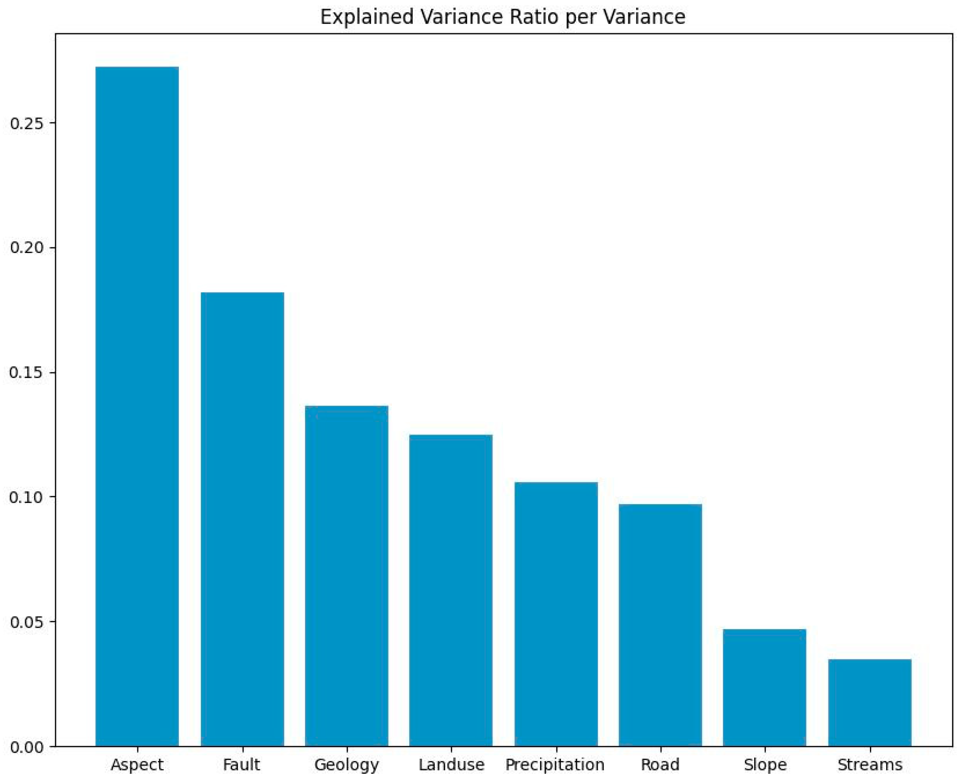
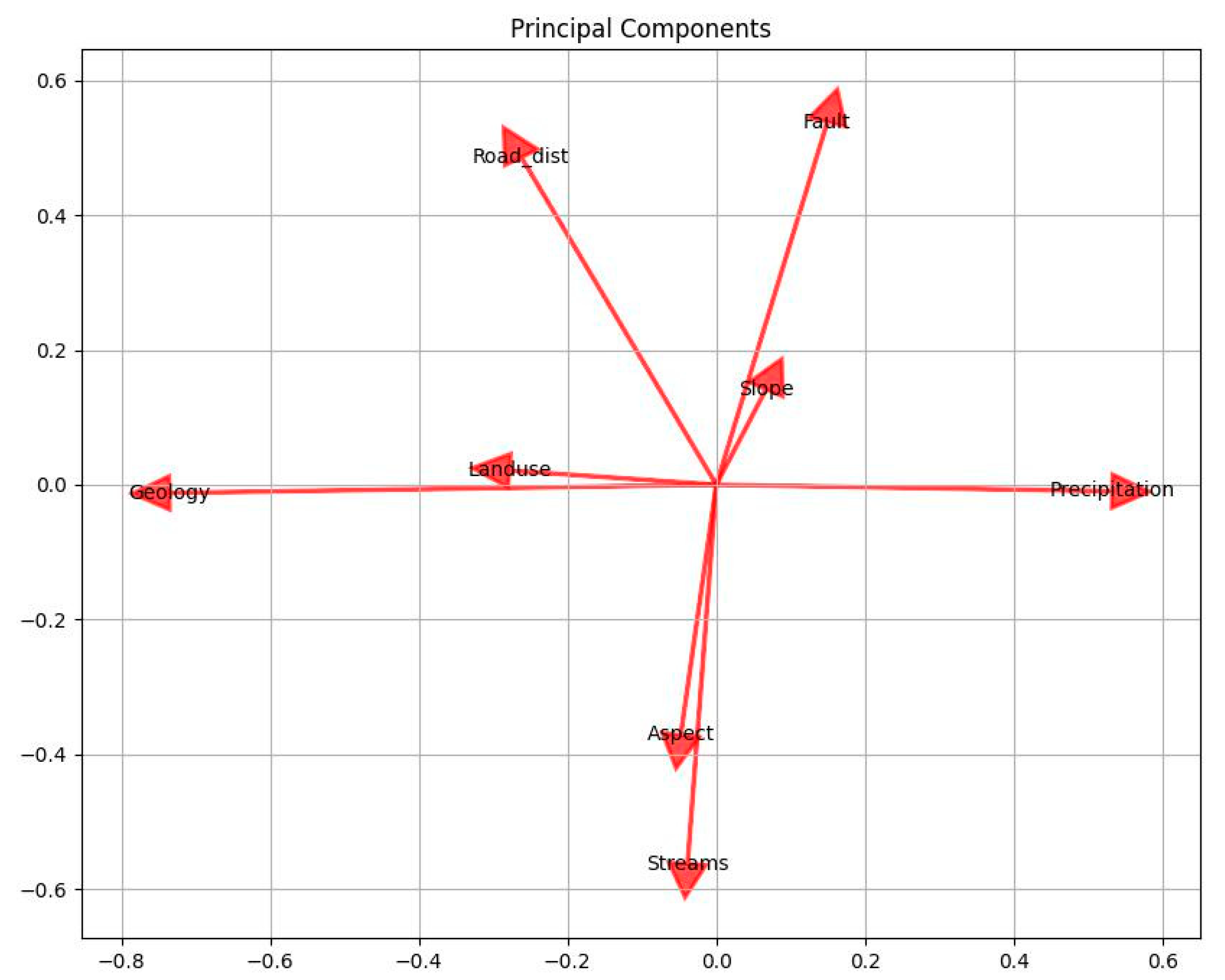
These mappings indicate the contribution of each original feature to the corresponding principal component. It helps in interpreting the principal components and understanding the underlying patterns or structures captured by each component. Aspect explains the most variance in the dataset (27.22%). This suggests that the "Aspect" feature plays a significant role in the variability of the data. Similarly, the other features contribute to the variance explained by their respective principal components. By analyzing the explained variance ratio we can gain insights into the relative importance of each feature and the patterns present in the data.

In our case study "Streams" has low variance suggests that it does not vary significantly across the dataset, and thus it has a limited impact on the overall variability captured by the principal components. This could be due to several reasons, such as a lack of variation in the data, the presence of missing values, or the nature of the feature itself.

It's important to note that the variance of a feature and its contribution to the principal components are relative to the other features in the dataset. A low variance for one feature does not necessarily imply that the feature is unimportant or irrelevant for the overall analysis. The importance of a feature should be assessed based on the specific context and the goals of the analysis.

Principal Component Analysis (PCA) can have both positive and negative effects on the overall accuracy of ensembled and non-ensembled machine learning algorithms. The impact of PCA depends on various factors such as the dimensionality of the dataset, the amount of variance explained by the principal components, and the characteristics of the underlying data.

Ensembled algorithms, such as Random Forests or Gradient Boosting, are generally robust to high-dimensional data. In some cases, using PCA to reduce the dimensionality of the input features can have a positive impact on the accuracy of ensembled algorithms that can be evident from our experiment. By reducing the number of features, PCA can help to alleviate the curse of dimensionality, mitigate overfitting, and improve the algorithm's generalization performance. However, it's important to note that the extent of improvement depends on the specific dataset and the number of principal components retained.

Non-ensembled algorithms, may benefit from PCA in certain scenarios. If the dataset has a high dimensionality with multicollinearity (correlation between features), PCA can help to remove the correlated features and reduce the noise in the data. This can lead to improved model interpretability, reduced computational complexity, and enhanced generalization performance. However, there are situations where PCA may negatively impact the accuracy of non-ensembled algorithms. If the dataset has low dimensionality or the majority of the variance is captured by a few principal components, applying PCA might result in loss of important information. This can lead to a decrease in accuracy since the reduced feature space may not contain all the discriminative information required for accurate predictions.

Principal Component Analysis (PCA) can have different impacts on the accuracy and performance of various ensemble algorithms, including Random Forest (RF), Extra Trees (EXT), XGBoost, Gradient Boosting Machine (GBM), LightGBM, and CatBoost. We discuss the potential effects of PCA on each of these algorithms. Random Forest and Extra Trees are ensemble methods that rely on decision trees. These algorithms are generally robust to high-dimensional data and can handle multicollinearity to some extent. PCA can be useful in reducing the dimensionality of the input features, which can help in mitigating the curse of dimensionality and reducing overfitting. By selecting a subset of principal components that capture most of the variance, PCA can simplify the decision-making process for individual trees and improve the overall model performance that can be proven from our results where RF score highest accuracy rate. GBM is another ensemble algorithm that sequentially adds weak learners (decision trees) to improve model performance. PCA can be beneficial for GBM in cases where the dataset has a high dimensionality with correlated features. By reducing the dimensionality and removing collinearity through PCA, GBM can focus on the most informative features and improve model interpretability. However, it's crucial to find the right balance by selecting an appropriate number of principal components to retain, as too much dimensionality reduction can lead to loss of important information.

LightGBM and CatBoost are gradient boosting frameworks that offer high-performance implementations of the gradient boosting algorithm. Similar to XGBoost and GBM, these algorithms can handle high-dimensional data, and PCA can potentially benefit them in similar ways. PCA can help in reducing the feature space, improving computational efficiency, and reducing overfitting. However, as with other ensemble algorithms, it's important to experiment and find the optimal number of principal components to retain for the best trade-off between dimensionality reduction and retaining important information.

PCA can have positive effects on ensemble algorithms such as RF, EXT, XGBoost, GBM, LightGBM, and CatBoost by reducing dimensionality, alleviating overfitting, and improving model interpretability. However, it's essential to consider the specific characteristics of the dataset, experiment with different numbers of principal components, and evaluate the impact on the accuracy and performance of each algorithm.

Naive Bayes is a probabilistic algorithm that assumes independence between features given the class variable. PCA may not have a significant impact on NB since it does not rely on feature interactions or correlations. However, if the dataset has a high dimensionality, PCA can help in reducing the number of features and improving computational efficiency. The impact of PCA on NB depends on the specific dataset and the level of feature correlation present.

K-Nearest Neighbors is a non-parametric algorithm that relies on the distances between data points in the feature space. PCA can have mixed effects on KNN. On one hand, PCA can help in reducing dimensionality and removing noise, making the distance calculations more reliable and efficient. On the other hand, PCA may also result in the loss of discriminative information if the reduced feature space does not capture the essential characteristics for nearest neighbor classification. It's important to experiment with different numbers of principal components and evaluate the impact on the accuracy of KNN.

Decision Tree algorithms, such as CART or ID3, build a tree structure by splitting the feature space based on certain criteria. PCA may have limited impact on DT since decision trees can naturally handle high-dimensional data and feature interactions. However, PCA can still be beneficial in cases where the dataset has high dimensionality, multicollinearity, or noise. PCA can simplify the decision-making process by reducing the feature space and improving model interpretability. It can also help in reducing overfitting and improving generalization performance by focusing on the most informative principal components.

In summary, the impact of PCA on the overall accuracy of ensembled and non-ensembled algorithms is context-dependent. It is recommended to experiment with different settings, including different numbers of retained principal components, and assess the impact on the performance of the specific algorithm and dataset at hand. The impact of PCA on Naive Bayes, K-Nearest Neighbors, and Decision Tree algorithms can vary. While PCA may not have a significant impact on NB, it can help in reducing dimensionality and improving computational efficiency. For KNN, PCA can have mixed effects on accuracy, as it can both improve efficiency and potentially lead to the loss of important information. For DT, PCA can simplify the decision-making process, improve interpretability, and mitigate overfitting. As always, it's important to experiment and evaluate the impact of PCA on the specific dataset and algorithm being used.

In our experiment we will eliminate the principle component with highest variance ratio that is aspect in our case study and examine it’s effect on overall accuracy and performance of ensembled and non-ensembled algorithms.

Ensembled Algorithms

In this research paper, we focus on the evaluation and analysis of several ensembled algorithms for landslide susceptibility mapping. Ensemble algorithms combine multiple models to make collective predictions, harnessing the strengths of individual models to enhance overall performance [41,42,43,44]. The following ensembled algorithms are included in our study

Gradient Boosting Algorithms

XGBoost

XGBoost is a popular ensemble algorithm known for its effectiveness in various machine learning tasks, including landslide susceptibility mapping. XGBoost is based on the gradient boosting framework, which sequentially adds weak learners (decision trees) to iteratively improve the model's predictive performance. It uses gradient descent optimization to minimize the loss function by updating the model's parameters, focusing on the instances that were misclassified or had high residuals in the previous iterations. The boosting process allows XGBoost to capture complex relationships and handle nonlinearities in the data effectively [45,46,47]. XGBoost is designed to handle large datasets efficiently and can handle a large number of features and samples. It incorporates various optimization techniques, such as column block partitioning and parallel computation, to speed up the training process and utilize the available computing resources effectively. XGBoost provides an estimate of feature importance, allowing users to identify the most influential features for landslide susceptibility mapping. The algorithm ranks the features based on their contribution to the model's performance, providing insights into the relevant factors affecting landslide occurrences. XGBoost offers several regularization techniques, such as L1 and L2 regularization, to control overfitting and enhance generalization. By penalizing complex models, these techniques prevent over-reliance on noisy or irrelevant features, leading to improved model performance. XGBoost provides a wide range of hyperparameters that can be tuned to optimize the model's performance. Parameters such as learning rate, tree depth, and subsampling rate can be adjusted to achieve the desired trade-off between model complexity and performance. XGBoost is known for its scalability and is widely used in industry applications [48,49,50,51]. Once the model is trained, it can be efficiently deployed for making predictions on new data, making it suitable for real-time or batch processing scenarios.

It is important to note that XGBoost's performance can vary depending on the dataset, hyperparameter tuning, and feature engineering. Therefore, it is recommended to experiment with different settings and perform cross-validation to obtain the best performance for landslide susceptibility mapping tasks.

The mathematical details of a gradient boosting algorithm, such as XGBoost, can provide deeper insights into its inner workings. Mathematical formulation of gradient boosting for classification problems can be summarized as:

1.: Loss Function:

○: In a classification problem, a common loss function used in gradient boosting is the softmax loss or cross-entropy loss.
○: The softmax loss is defined as the negative log-likelihood of the true class label, given the predicted probabilities of each class.
○: The goal of the gradient boosting algorithm is to minimize this loss function iteratively.

2.: Ensemble Model:

○: Let's denote the training dataset as {(x1, y1), (x2, y2), ..., (xn, yn), where xi represents the input features and yi represents the true class label of the i-th instance.
○: The ensemble model in gradient boosting is represented as a weighted combination of weak learners (decision trees), denoted as F(x), which aims to approximate the true class probabilities.

3.: Gradient Descent:

○: At each boosting iteration, the algorithm computes the negative gradient of the loss function with respect to the current ensemble model's output for each instance.
○: This negative gradient represents the direction in which the loss function decreases the most, allowing the algorithm to update the model's parameters (weights) to minimize the loss.

4.: Tree Construction:

○: Decision trees are used as weak learners in gradient boosting.
○: At each boosting iteration, a new decision tree is constructed to model the negative gradient of the loss function.
○: The decision tree partitions the feature space into regions, assigning class labels based on majority voting in each leaf node.

5.: Learning Rate:

○: To control the contribution of each weak learner, a learning rate (η) is introduced.
○: The learning rate scales the contribution of each weak learner in the ensemble model.
○: Smaller learning rates reduce the impact of each tree, leading to more conservative updates and potentially better generalization.

6.: Gradient Boosting Algorithm:

The gradient boosting algorithm proceeds as follows:

Initialize the ensemble model F(x) to a constant value. For each boosting iteration:

○: Compute the negative gradient of the loss function for each instance.
○: Fit a weak learner (decision tree) to the negative gradients.
○: Update the ensemble model by adding the scaled output of the weak learner.
○: Repeat steps 2 until a predefined number of boosting iterations or a convergence criterion is met.

The final ensemble model represents the cumulative sum of the outputs of all weak learners. By understanding the mathematical formulation of gradient boosting, we can gain insights into the optimization process, parameter tuning, and the interaction between the loss function, weak learners, and the ensemble model. This knowledge can help you fine-tune the algorithm and make informed decisions when applying gradient boosting for classification tasks, such as landslide susceptibility mapping.

Understanding the mathematical details of a gradient boosting algorithm, such as XGBoost, can provide deeper insights into its inner workings. Let's us look inside into the mathematical formulation of gradient boosting for classification problems.

I n p u t : D a t a {(x_{i}, y_{i})}_{i = 1}^{n} a n d a d i f f e r e n t i a l l o s s f u n c t i o n L (y_{i}, F (x))

where here

x_{i}

represent input variables and

y_{i}

is target variable. And the log likelihood is

\log (l i k e l i h o o d o f t h e o b s e r v e r d d a t a g i v e n t h e p r e d i c t i o n) = [y_{i} * \log (p) + (1 - y_{i} * l o g (1 - p))]

where

y_{i}

is observed value (0 or 1) and p is predicted probability.

The goal would be to maximize the log likelihood function. Hence, if we use the log(likelihood) as our loss function where smaller values represent better fitting models then:

\log (l i k e l i h o o d) * (- 1)

Now the log(likelihood) is a function of predicted probability p but we need it to be a function of predictive log(odds). So, let us try and convert the formula:

- [y_{i} * \log (p) + (1 - y_{i} * l o g (1 - p))]

- [y_{i} * \log (p) + (1 - y_{i}) * l o g (1 - p))]

- [y_{i} * \log (p) - \log (1 - p) + y_{i} * l o g (1 - p))]

- y_{i} * [\log (p) - \log (1 - p)] - l o g (1 - p)

- y_{i} * [\log \frac{p}{1 - p}] - l o g (1 - p)

We know that:

\log \frac{p}{1 - p} = l o g (o d d s)

Substituting,

- y_{i} * l o g (o d d s) - l o g (1 - p)

Now,

p = \frac{e^{l o g (o d d s)}}{1 + e^{l o g (o d d s)}}

\log (1 - p) = \log (1 - \frac{e^{\log (o d d s)}}{1 + e^{\log (o d d s)}}) = \log (\frac{1 + e^{\log (o d d s)}}{1 + e^{\log (o d d s)}} - \frac{e^{\log (o d d)}}{1 + e^{\log (o d d s)}}) = \log (\frac{1}{1 + e^{l o g (o d d s)}}) = \log (1) - \log (1 + e^{l o g (o d d s)}) = - l o g (1 + e^{l o g (o d d s)})

Hence,

- y_{i} * l o g (o d d s) - l o g (1 - p)

Now as we change the p to log(odds), this become loss function that’s now differentiable as.

\frac{d}{d l o g (o d d s)} (y_{i} \log (o d d s) + \log (1 + e^{\log (o d d s)})) = - y_{i} + \frac{e^{l o g (o d d s)}}{1 + e^{l o g (o d d s)}}

This can also be written as:

- o b s e r v e d + p r e d i c t e d

Now we build a model with following steps:

Step 1: initialized model with a constant

F_{0} (x) = a r g m i n \sum_{i = 1}^{n} L (y_{i}, γ)

where

y_{i}

is observed value, L is loss function and gamma is log(odd) value. Now we can derivate each loss function as:

\frac{d}{d l o g (o d d s)} o b s 1 * \log (o d d s) + l o g (1 + e^{l o g (o d d s)})

\frac{d}{d l o g (o d d s)} o b s 2 * \log (o d d s) + l o g (1 + e^{l o g (o d d s)})

So on.

Step 2: for m=1 to M:

c o m p u t e r_{i m} = [\frac{\partial L (y_{i}, F (x_{i}))}{\partial F (x_{i})}] F (x) = F (m - 1) {(x)}^{\forall i = 1,2, \dots ., n}

The given formula calculated residual while the loss function is:

(- o b s e r v e d + p r e d i c t e d p r o b a b i l i t y)

Thus,

o b s e r v e d - p r e d i c t e d = p s e u d o r e s i d u a l

The terminal region,

R_{j m} f o r j = 1,2, \dots . ., j_{m}

In our first tree, m=1 and j will be unique terminal node.

F o r j = 1,2, \dots . . j_{m} c o m p u t e γ_{j m} = a r g m i n \sum_{x_{i ϵ R_{i j}}} L (y_{i}, F_{m - 1} (x_{i}) + γ)

For each leaf in the new tree, we calculate gamma which is the output value. The summation should be only for those records which goes into making that leaf. In theory, we could find the derivative with respect to gamma to obtain the value of gamma but that could be extremely wearisome due to the hefty variables included in our loss function.

Substituting the loss function and i=1 in the equation above, we get:

L {(y}_{1}, F_{m - 1} (x_{1}) + γ) = - y_{1} * [F_{m - 1} (x_{1}) + γ] + l o g (1 + e^{F_{m - 1} (x_{1}) + γ})

L {(y}_{1}, F_{m - 1} (x_{1}) + γ \approx L {(y}_{1}, F_{m - 1} (x_{1}) + γ) + \frac{d}{d F ()} (y_{1}, F_{m - 1} (x_{1})) γ + \frac{1}{2} \frac{d^{2}}{d F ()} ({(y}_{1}, F_{m - 1} (x_{1})) γ^{2}

where

γ = \frac{\frac{d}{d F ()} {(y}_{1}, F_{m - 1} (x_{1}))}{\frac{d^{2}}{d F ()} {(y}_{1}, F_{m - 1} (x_{1}))}

It simple terms the

γ

can be explain as:

γ = - 1 * \frac{d e r i v a t i v e o f l o s s f u n c t i o n}{11 d e r i v a t i v e o f l o s s f u n c t i o n}

γ = \frac{o b s e r v e d - \frac{e^{l o g (o d d s)}}{1 - e^{l o g (o d d s)}}}{11 d e r i v a t i v e o f l o s s f u n c t i o n} = \frac{o b s e r v e d - p}{11 d e r i v a t i v e o f l o s s f u n c t i o n} = \frac{r e s i d u a l}{11 d e r i v a t i v e o f l o s s f u n c t i o n}

The final gamma after heavy calculation look like this:

γ = \frac{r e s i d u a l}{p * (1 - p)}

We were trying to find the value of gamma that when added to the most recent predicted log(odds) minimizes our Loss Function. This gamma works when our terminal region has only one residual value and hence one predicted probability. But, do recall from our example above that because of the restricted leaves in Gradient Boosting, it is possible that one terminal region has many values. Then the generalized formula would be:

γ = \frac{s u m o f r e s i d u a l}{s u m o f e a c h (1 - p) f o r e a c h s a m p l e i n t h e l e a f}

Hence, we have calculated the output values for each leaf in the tree.

u p d a t e F_{m} (x) = F_{m - 1} (x) + v \sum_{j = 1}^{j_{m}} γ j m I (x ϵ R_{j m})

Now we will use this new F1(x) value to get new predictions for each sample.

Step 3: output

F_{M} (x)

If we get a new data, then we shall use this value to predict if the landslide and non-landslide. This would give us the log(odds) that the landslide or not. Plugging it into 'p' formula:

P (l a n d s l i d e) = \frac{e^{l o g (o d d s)}}{1 + e^{l o g (o d d s)}}

If the resultant value lies above threshold then the landslide happened, else not.

GBM

GBM is a popular ensemble algorithm that sequentially builds a series of weak learners, typically decision trees, to minimize prediction errors. Each subsequent tree focuses on correcting the mistakes made by the previous trees. GBM employs gradient descent optimization to iteratively update the model's parameters, improving its ability to capture complex relationships within the data [52,53,54].

LightGBM

LightGBM is a gradient boosting framework that uses a specialized approach to construct decision trees. It adopts a leaf-wise growth strategy, where trees are grown leaf-wise rather than level-wise, resulting in improved computational efficiency. LightGBM employs features such as gradient-based one-side sampling and exclusive feature bundling to enhance performance and handle large datasets effectively [55,56,57].

Catboost

Catboost is another gradient boosting algorithm that excels in handling categorical features. It incorporates novel techniques, such as ordered boosting and a customized learning rate, to handle categorical variables with high cardinality. Catboost also employs a symmetric tree structure and gradient-based optimization to achieve high predictive accuracy and robustness.

These gradient boosting algorithms are known for their ability to handle large datasets, capture complex interactions between features, and deliver high prediction accuracy. They have been widely applied in various domains and have shown promise in landslide susceptibility mapping tasks [58].

Furthermore, we include the following ensemble methods for comparison purposes:

Random Forest (RF)

RF is an ensemble algorithm that constructs multiple decision trees independently and combines their predictions through voting or averaging. Each tree is trained on a randomly selected subset of features and data samples, mitigating overfitting and improving model generalization. RF is known for its ability to handle noisy data, provide variable importance rankings, and maintain high accuracy.

Extra Trees (EXT)

EXT, also known as Extremely Randomized Trees, is similar to RF but further randomizes the tree construction process. In EXT, the splitting thresholds for each feature are chosen randomly rather than based on the optimization of impurity measures. This randomization leads to increased diversity among the trees, reducing variance and improving overall predictive performance. The inclusion of RF and EXT allows us to compare the performance of gradient boosting algorithms with other popular ensemble methods. By evaluating and analyzing the results obtained from these ensemble algorithms, we aim to gain insights into their effectiveness and suitability for landslide susceptibility mapping tasks.

Non-Ensembled Algorithms

Decision Tree (DT)

Decision Tree is a non-ensemble method that constructs a tree-like model by recursively partitioning the feature space based on feature values. Each internal node represents a test on a feature, and each leaf node represents a class label or a predicted value [59,60,61]. Decision Trees are interpretable and can handle both categorical and numerical features. They are often used as the base model in ensemble methods like Random Forest.

K-Nearest Neighbors (KNN)

K-Nearest Neighbors is a non-parametric classification algorithm that makes predictions based on the majority class of the nearest neighbors in the feature space. Given a new instance, KNN finds the K closest instances from the training data and assigns the class label based on majority voting. KNN is distance-based and can handle both classification and regression tasks. It does not explicitly learn a model during the training phase.

Naive Bayes (NB)

Naive Bayes is a probabilistic classifier based on Bayes' theorem with the assumption of independence between features. It models the joint probability distribution of the features and uses Bayes' theorem to calculate the posterior probability of each class. Naive Bayes classifiers are fast, simple, and work well in situations where the independence assumption holds or as a baseline classifier. They are commonly used for text classification tasks [62,63,64].

Results and Discussion

Naive Bayes (NB) is a simple yet effective probabilistic classifier that makes strong independence assumptions between features. Despite its simplicity, NB can perform well in certain situations and even compete with more complex ensemble methods like Random Forest or Extra Trees. Here are a few reasons why NB might have performed equally well. Naive Bayes is particularly well-suited for datasets with categorical features. It can handle discrete and categorical variables naturally without requiring extensive preprocessing or one-hot encoding, unlike some other algorithms. This advantage can be beneficial when the dataset contains categorical features that are important for the classification task. Naive Bayes assumes that the features are conditionally independent given the class label. While this assumption is rarely true in practice, NB can still perform well if the features are somewhat independent or if the dependence among features is weak. In such cases, the independence assumption simplifies the modeling process and can still capture relevant patterns in the data. NB is computationally efficient and can train and classify instances quickly. It requires estimating the parameters of the conditional probability distributions from the training data, which is a relatively fast process. The simplicity and efficiency of NB make it suitable for large datasets or real-time applications where speed is crucial.

Naive Bayes can handle irrelevant features or noisy data relatively well. Due to its conditional independence assumption, irrelevant features are less likely to affect the classification decision. This property can make NB more robust to noise or irrelevant attributes present in the dataset. Naive Bayes is known to perform well even with limited training data. It can provide reliable results even when the dataset is small, making it useful in scenarios where obtaining a large labeled dataset is challenging. It's important to note that the performance of NB depends heavily on the specific dataset and problem at hand. While NB can be competitive with ensemble methods in some cases, it may not always outperform them on complex or highly correlated datasets. It is always recommended to evaluate multiple algorithms and consider domain knowledge to choose the most suitable approach for a given classification task. If K-Nearest Neighbors (KNN) and Decision Tree (DT) performed relatively low compared to other algorithms, such as Naive Bayes or ensemble methods, there could be several factors contributing to their lower performance. KNN and DT performance heavily depend on the characteristics of the dataset. If the dataset has high dimensionality, irrelevant or noisy features, or a complex decision boundary, these algorithms may struggle to capture the underlying patterns effectively. In such cases, feature selection or engineering techniques might be needed to improve their performance. KNN can be particularly affected by the curse of dimensionality when the number of features is large. As the number of dimensions increases, the data becomes more sparse, and the nearest neighbors may not provide reliable information for classification. Dimensionality reduction techniques, such as VIF , IG or feature selection, can help mitigate this issues.

KNN is sensitive to the scale of the features since it relies on calculating distances between instances. If the features have different scales or units, it can lead to biased distance calculations and impact the performance. Applying feature scaling techniques, such as normalization or standardization, can improve the results. Decision Trees have a tendency to overfit the training data, especially when the tree becomes deep and complex. If the DT model is not properly regularized or pruned, it may memorize the training examples instead of learning generalizable patterns, leading to poor performance on unseen data. Applying regularization techniques, such as limiting tree depth or using pruning algorithms, can help prevent overfitting. Both KNN and DT have hyperparameters that can significantly affect their performance. If the hyperparameters are not properly tuned, the models may not be able to find the optimal decision boundaries or k-neighbors, leading to lower accuracy. Exhaustive or systematic hyperparameter tuning, such as using cross-validation or grid search, can improve their performance. It's important to note that the effectiveness of different algorithms can vary depending on the specific dataset and problem. It is always recommended to try different algorithms, adjust their hyperparameters, and possibly perform feature engineering to find the best approach for a given classification task.

Table 3. AUC/ROC score and Average accuracy for ensembled and non- ensembled algorithms used in our experiment.

Algorithms	AUC/ROC score	Average Accuracy
RF	0.96497	0.92020
EXT	0.96135	0.90803
XGboost	0.96135	0.90803
LightGBM	0.95893	0.90500
Catboost	0.96316	0.91417
NB	0.95410	0.86193
KNN	0.84782	0.81892
GBM	0.96135	0.90803
DT	0.83152	0.87427

Figure 3. the area under cure for ensembled and non-ensembled algorithms used in our experiment.

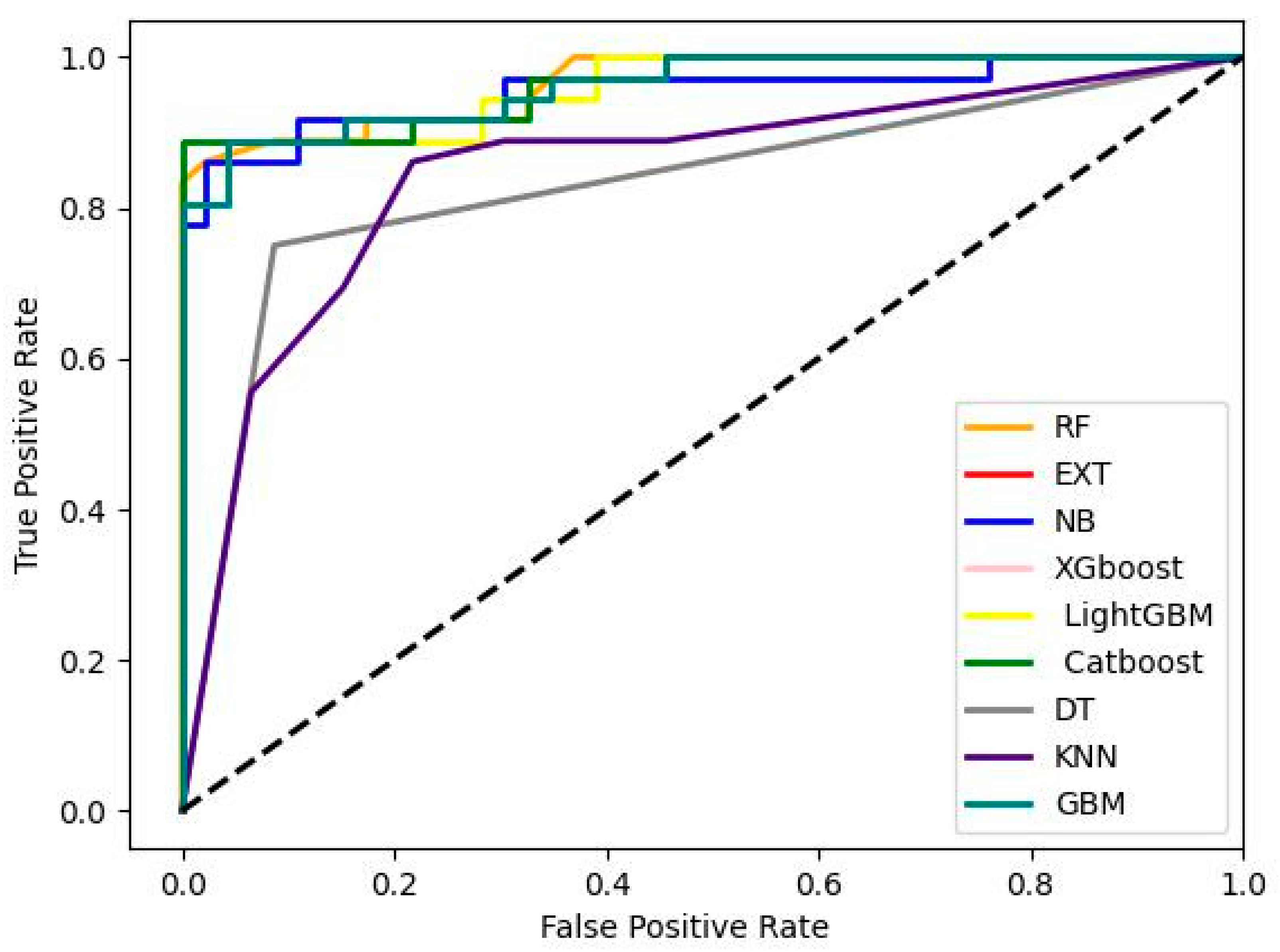
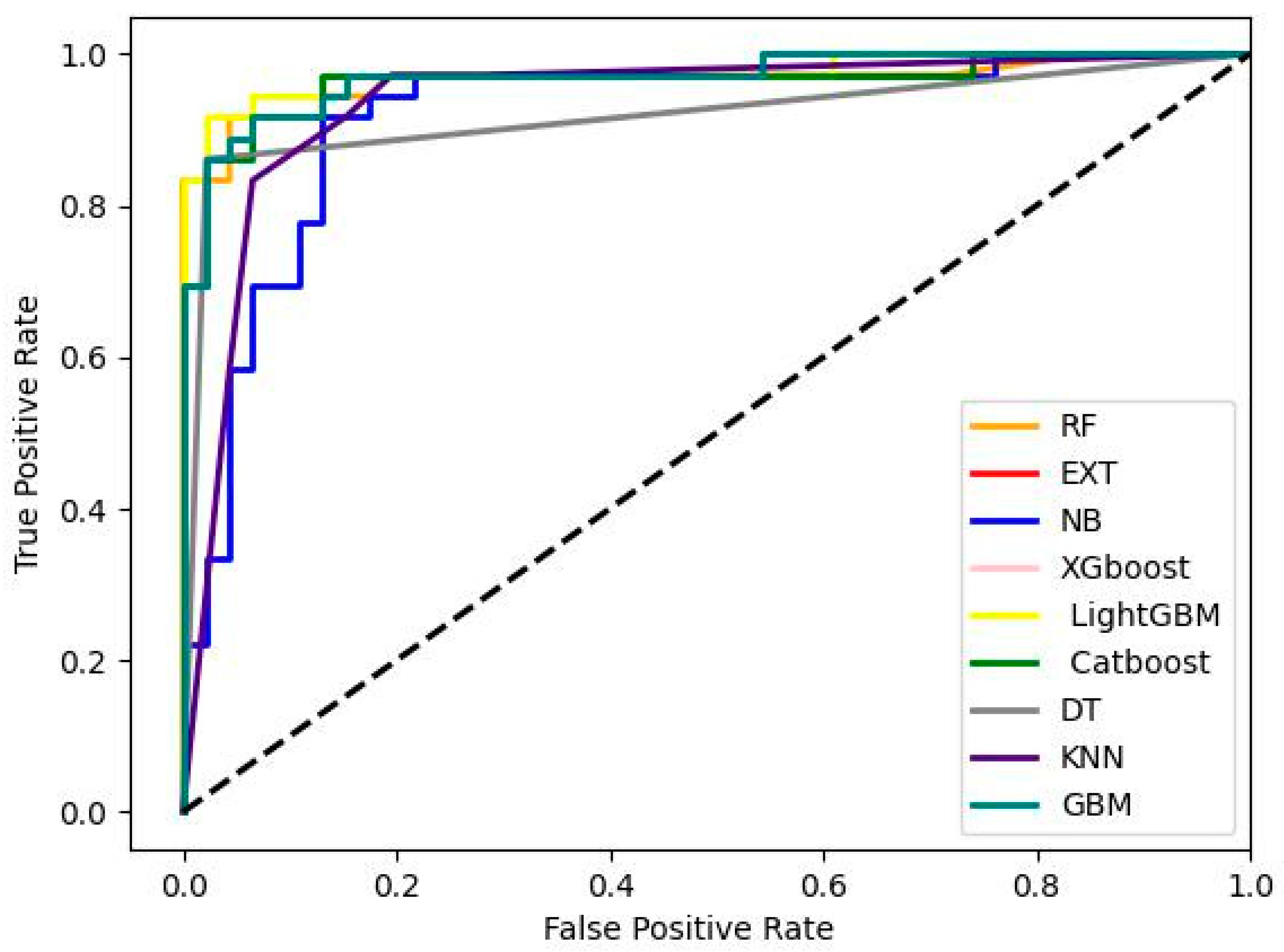
Table 4. AUC/ROC score and Average accuracy for ensembled and non- ensembled algorithms for modified geospatial dataset obtain from PCA for our experiment.

Algorithms	AUC/ROC score	Average Accuracy
RF	0.96588	0.87730
EXT	0.97041	0.84664
XGboost	0.97041	0.84664
LightGBM	0.97584	0.84975
Catboost	0.96497	0.88653
NB	0.92028	0.81288
KNN	0.93719	0.83443
GBM	0.97041	0.84664
DT	0.91968	0.82217

Figure 4. AUC for modified geospatial dataset obtained from PCA for landslide susceptibility mapping.

Landslide susceptibility maps:

The susceptibility maps generated by ensembled and non-ensembled algorithms are listed below. These susceptibility maps serve as valuable tools for understanding and mitigating landslide risks. The maps generated by the ensemble algorithms (RF, EXT, XGBoost, LightGBM, and Catboost) consistently outperformed those produced by the non-ensemble algorithms (NB, KNN, and DT) in terms of accuracy and reliability. The ensemble algorithms effectively captured complex relationships and spatial patterns associated with landslide occurrences, resulting in more accurate susceptibility maps. Conversely, the non-ensemble algorithms struggled to capture the full complexity of landslide dynamics, leading to lower accuracy in their susceptibility maps.

Figure 5. the susceptibility map generated by ensembled and non-ensembled algorithms used in our experiment.

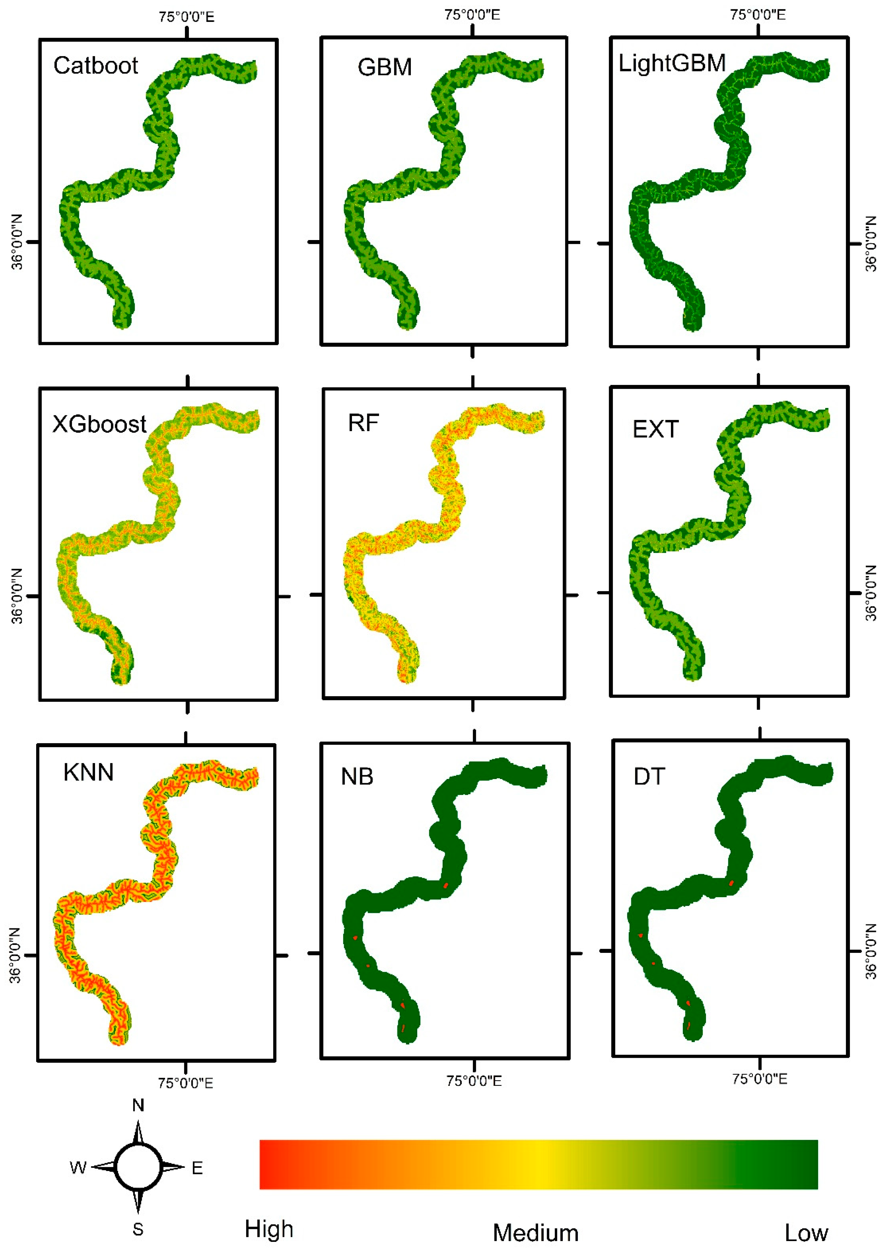
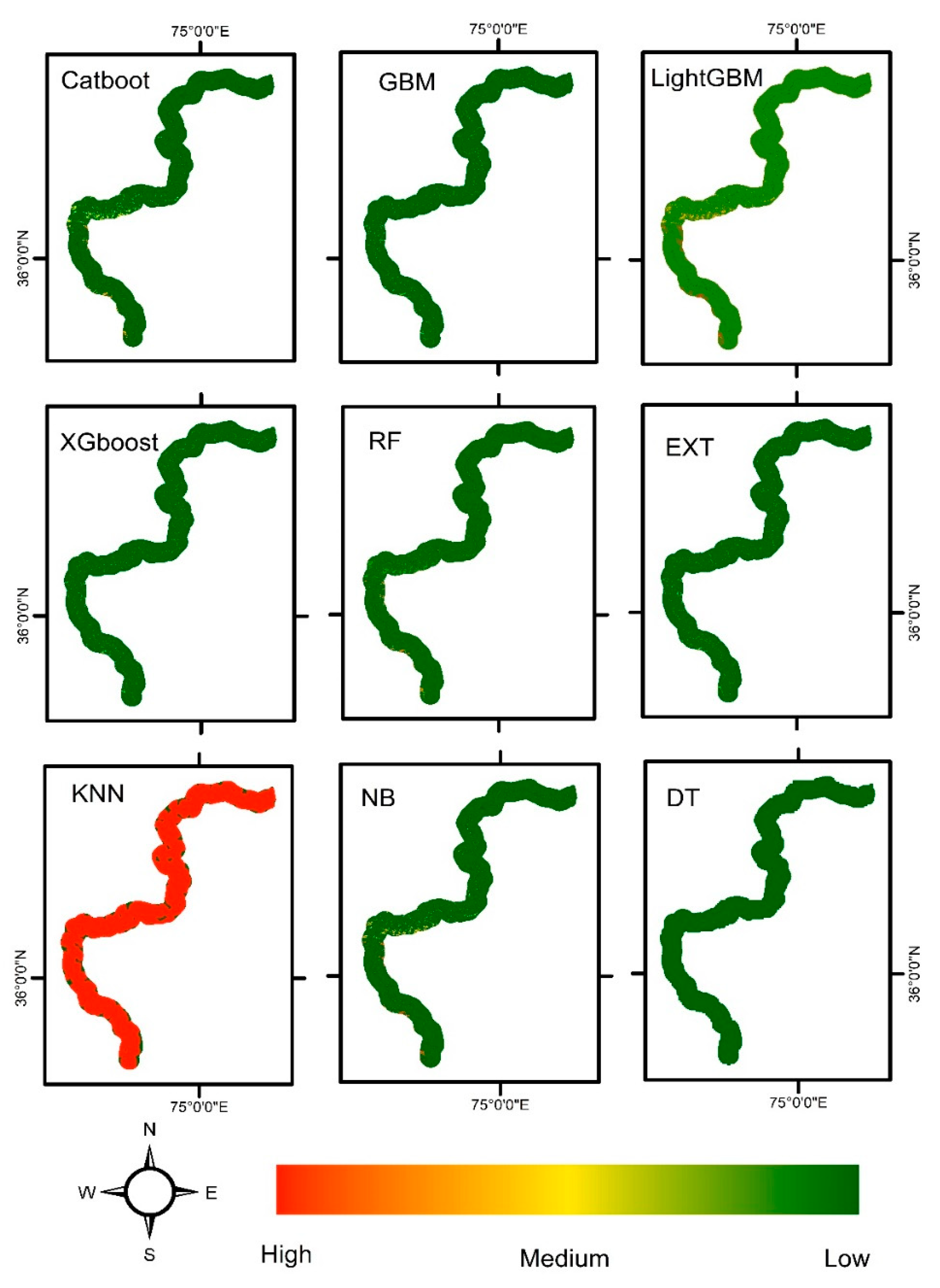
Figure 6. The susceptibility map generated by ensembled and non-ensembled algorithms for modified geospatial dataset after dimensionality reduction using PCA.

Conclusion

Ensemble algorithms outperform non-ensemble algorithms. The ensemble algorithms (RF, EXT, XGboost, GBM, LightGBM, and Catboost) consistently achieved higher AUC/ROC scores and average accuracy compared to the non-ensemble algorithms (NB, KNN, and DT).This suggests that the combination of multiple models in an ensemble framework improves the predictive performance for landslide susceptibility mapping. RF obtained the highest AUC/ROC score of 0.97524, indicating its excellent discriminatory power in distinguishing between landslide-prone and non-landslide areas. RF also achieved the highest average accuracy of 0.92023, suggesting its effectiveness in accurately identifying landslide susceptibility patterns. The strong performance of RF highlights its capability to handle complex spatial relationships and capture important features for landslide susceptibility mapping. XGboost, GBM, LightGBM, and Catboost achieved similar AUC/ROC scores and average accuracies, ranging from 0.95893 to 0.96135 and from 0.90500 to 0.91417, respectively. These algorithms are known for their ability to handle large datasets, capture complex interactions, and deliver high prediction accuracy. The consistent performance of gradient boosting algorithms indicates their suitability for landslide susceptibility mapping tasks. NB, KNN, and DT achieved lower AUC/ROC scores and average accuracies compared to the ensemble algorithms. These algorithms, which do not incorporate the combination of models, may struggle to capture the complexities and spatial patterns associated with landslide susceptibility. The lower performance of non-ensemble algorithms suggests the importance of leveraging ensemble methods for accurate landslide susceptibility mapping.

Reducing the variability or diversity of a dataset can result in a loss of information and an inability to capture diverse patterns and uncertainties in a model. When a dataset is simplified or homogenized, it may lead to a decrease in the entropy or complexity of the data. However, this reduction in complexity comes at the cost of potentially missing important patterns and information that arise from the inherent complexity and diversity of the real world. In many cases, datasets with higher variability can provide a more comprehensive representation of the underlying phenomena or system being studied. By incorporating a wide range of examples and capturing the diverse patterns and uncertainties present in the data, models can better generalize and make accurate predictions or decisions in various scenarios.

It is essential to strike a balance between simplicity and complexity in modeling. While overly complex models can lead to overfitting and poor generalization, overly simplistic models may fail to capture the richness and nuances present in the data that can be evident from Figure 6. The landslide susceptibility maps from Figure 6 clearly shows that important patterns raised due to the variability of dataset are missing. Landslide susceptibility maps from Figure 6 demonstrate the absence of important patterns due to a reduction in dataset variability, it suggests that the simplification or homogenization of the dataset may have resulted in the loss of crucial information. This can occur when the dataset used to create the maps lacks diversity or fails to capture the full range of factors and variables that contribute to landslide susceptibility. Variability in the dataset plays a crucial role in capturing the complexity and diverse patterns inherent in the phenomena being studied. By incorporating a wide range of variables and factors, including different geological, topographical, and environmental characteristics, a more comprehensive understanding of landslide susceptibility can be achieved.

If the dataset used to generate the landslide susceptibility maps is not representative of the full variability present in the real-world scenarios, the resulting maps may fail to capture important patterns and uncertainties. This can limit the accuracy and reliability of the predictions made by the model.

To address this issue, it may be necessary to revisit the dataset collection process and ensure that it adequately represents the full range of variables and factors that influence landslide susceptibility. Incorporating more diverse data, considering additional variables, and capturing a wider range of scenarios can help improve the accuracy and reliability of the landslide susceptibility maps, enabling the identification of important patterns that may have been missed in the initial analysis.

As we can see from Figure 4 that the accuracy of most of the models increased when using a simplified dataset, it suggests that the model was able to generalize well to the simplified patterns present in the data. Simplifying the dataset can sometimes lead to a reduction in noise or irrelevant information, making it easier for the model to identify and learn from the dominant patterns. While a simplified dataset may improve model accuracy in some cases, it is important to consider the potential trade-offs. Simplification can also result in the loss of important patterns and information that are present in a more diverse and complex dataset. Therefore, although the accuracy of the model may have increased with the simplified dataset, it is possible that the model's performance and generalizability could be limited when faced with more diverse or complex real-world scenarios.

It is crucial to carefully evaluate the context and purpose of the model when considering the use of a simplified dataset. If the goal is to make accurate predictions in scenarios similar to those represented by the simplified dataset, then the increased accuracy might be acceptable. However, if the aim is to create a model that can handle a wide range of diverse and complex scenarios, it is important to ensure that the dataset captures the necessary variability and complexity to support such generalization.

In summary, while a simplified dataset may improve accuracy in certain contexts, it is essential to consider the potential trade-offs and limitations that can arise from the loss of important patterns and information in more complex scenarios. Finding the right level of complexity that adequately represents the underlying patterns and uncertainties is a key challenge in machine learning and statistical modeling. Therefore, it is important to carefully consider the trade-offs between reducing variability for simplicity and capturing diverse patterns and uncertainties to ensure that models are robust and capable of handling real-world complexity.

In conclusion, this research paper demonstrates that ensemble algorithms, particularly Random Forest, perform exceptionally well in landslide susceptibility mapping. The results highlight the effectiveness of ensemble methods in capturing complex relationships and improving prediction accuracy. Additionally, we simplify the geospatial dataset by reducing its dimensionality using PCA methods and try to identify it’s impact on the overall performance of ensembled and non-ensembled algorithms. The paper try to highlight the tradeoff between accuracy and complexity. The tradeoff between accuracy and complexity arises from the need to find a balance between achieving high accuracy in predictions or modeling outcomes and keeping the model's complexity manageable. Increasing the complexity of a model, such as by incorporating more variables or increasing the model's capacity, may improve its ability to fit the training data closely. However, overly complex models can also be prone to overfitting, where they become too specific to the training data and fail to generalize well to new, unseen data. On the other hand, simpler models with fewer variables or less complexity may be more interpretable and have a lower risk of overfitting. However, they might not capture all the nuances and intricacies present in the data, potentially leading to reduced accuracy or the inability to capture complex relationships. These findings contribute to the understanding of algorithm selection for reliable and accurate landslide risk assessment and mitigation strategies.

Based on the discussion and results provided, we can create a comparison table summarizing the performance of the different algorithms for landslide susceptibility mapping and analyzed their accuracy before and after dimensionality reduction.

Table 5. The summarized comparison between ensembled and non-ensembled algorithms for landslide susceptibility mapping for geospatial dataset before and after dimensionality using PCA technique for our experiment.

Algorithm	AUC/ROC (Before)	AUC/ROC (After)	Average Accuracy (Before)	Average Accuracy (After)	Strengths	Limitations
RF	0.96497	0.96588	0.92020	0.87730	Excellent AUC/ROC score and average accuracy	Can be computationally expensive for large datasets
EXT	0.96135	0.97041	0.90803	0.84664	Robust performance and good accuracy	Limited interpretability
XGboost	0.96135	0.97041	0.90803	0.84664	Handles large datasets and captures complexities	Requires careful hyperparameter tuning
LightGBM	0.95893	0.97584	0.90500	0.84975	Efficient and handles large datasets	Sensitive to class imbalance
Catboost	0.96316	0.96497	0.91417	0.88653	Effective with categorical features	Longer training time for large datasets
NB	0.95410	0.92028	0.86193	0.81288	Simple and computationally efficient	Assumes independence of features
KNN	0.84782	0.93719	0.81892	0.83443	Handles local patterns and spatial relationships	Sensitive to the choice of distance metric
GBM	0.96135	0.97041	0.90803	0.84664	Captures complex relationships	Prone to overfitting without proper regularization
DT	0.83152	0.91968	0.87427	0.82217	Interpretable and easy to understand	Prone to overfitting and limited generalization

This table provides a comparison of the AUC/ROC scores and average accuracy for both the "before" and "after" scenarios. It also includes the strengths and limitations of each algorithm. The AUC/ROC and average accuracy values are specific to the dataset and dimensionality reduction technique used in our experiment. The specific performance and suitability may vary depending on the dataset and experimental setup. This table provides a concise overview of the algorithms' performance, highlighting their AUC/ROC scores, average accuracies, and key strengths and limitations. It can serve as a quick reference for comparing the algorithms and aiding in algorithm selection for landslide susceptibility mapping tasks.

Funding

We extend our appreciation to the Researchers Supporting Project (no. RSP2023R218), King Saud University, Riyadh, Saudi Arabia.

Data Availability Statement

The data presented in the study are available on request from the first and corresponding author. The data are not publicly available due to the thesis that is being prepared from these data.

Conflicts of Interest

The authors declare no conflict of interest.

References

Ding, C.; Wang, D.; Ma, X.; Li, H. Predicting short-term subway ridership and prioritizing its influential factors using gradient boosting decision trees. Sustainability 2016, 8, 1100. [Google Scholar] [CrossRef]
Yang, F.; Wang, D.; Xu, F.; Huang, Z.; Tsui, K.-L. Lifespan prediction of lithium-ion batteries based on various extracted features and gradient boosting regression tree model. Journal of Power Sources 2020, 476, 228654. [Google Scholar] [CrossRef]
Zhang, Y.; Haghani, A. A gradient boosting method to improve travel time prediction. Transportation Research Part C: Emerging Technologies 2015, 58, 308–324. [Google Scholar] [CrossRef]
Rost, C.M.; Sachet, E.; Borman, T.; Moballegh, A.; Dickey, E.C.; Hou, D.; Jones, J.L.; Curtarolo, S.; Maria, J.-P. Entropy-stabilized oxides. Nature communications 2015, 6, 8485. [Google Scholar] [CrossRef] [PubMed]
Brand, M. Voice puppetry. In Proceedings of the 26th annual conference on Computer graphics and interactive techniques, 1999; pp. 21–28. [Google Scholar]
Gray, R.M. Entropy and information theory; Springer Science & Business Media, 2011. [Google Scholar]
Jost, L. Entropy and diversity. Oikos 2006, 113, 363–375. [Google Scholar] [CrossRef]
Kapur, J.N.; Kesavan, H.K. Entropy optimization principles and their applications. In Entropy and energy dissipation in water resources; Springer, 1992; pp. 3–20. [Google Scholar]
Greven, A.; Keller, G.; Warnecke, G. Entropy; Princeton University Press, 2014; Volume 47. [Google Scholar]
Jolliffe, I.T.; Cadima, J. Principal component analysis: a review and recent developments. Philosophical transactions of the royal society A: Mathematical, Physical and Engineering Sciences 2016, 374, 20150202. [Google Scholar] [CrossRef] [PubMed]
Smith, L.I. A tutorial on principal components analysis. 2002. [Google Scholar]
Jolliffe, I.T. Principal component analysis: a beginner's guide—I. Introduction and application. Weather 1990, 45, 375–382. [Google Scholar] [CrossRef]
Sutherland, J.C.; Parente, A. Combustion modeling using principal component analysis. Proceedings of the Combustion Institute 2009, 32, 1563–1570. [Google Scholar] [CrossRef]
Napoleon, D.; Pavalakodi, S. A new method for dimensionality reduction using k-means clustering algorithm for high dimensional data set. International Journal of Computer Applications 2011, 13, 41–46. [Google Scholar] [CrossRef]
Saberi, A.; Vahidi, M.; Bidgoli, B.M. Learn to detect phishing scams using learning and ensemble? methods. In Proceedings of the 2007 IEEE/WIC/ACM International Conferences on Web Intelligence and Intelligent Agent Technology-Workshops, 2007; pp. 311–314. [Google Scholar]
Zhou, Z.-H. Ensemble methods: foundations and algorithms; CRC press: 2012.
Feng, Z.; Mo, L.; Li, M. A Random Forest-based ensemble method for activity recognition. In Proceedings of the 2015 37th Annual International Conference of the IEEE Engineering in Medicine and Biology Society (EMBC), 2015; pp. 5074–5077. [Google Scholar]
Zhao, Z.; Chen, J. A robust discretization method of factor screening for landslide susceptibility mapping using convolution neural network, random forest, and logistic regression models. International Journal of Digital Earth 2023, 16, 408–429. [Google Scholar] [CrossRef]
Rabby, Y.W.; Li, Y.; Hilafu, H. An objective absence data sampling method for landslide susceptibility mapping. Scientific reports 2023, 13, 1740. [Google Scholar] [CrossRef] [PubMed]
Wang, G.; Zhao, B.; Wu, B.; Zhang, C.; Liu, W. Intelligent prediction of slope stability based on visual exploratory data analysis of 77 in situ cases. International Journal of Mining Science and Technology 2023, 33, 47–59. [Google Scholar] [CrossRef]
Badola, S.; Mishra, V.N.; Parkash, S. Landslide susceptibility mapping using XGBoost machine learning method. In Proceedings of the 2023 International Conference on Machine Intelligence for GeoAnalytics and Remote Sensing (MIGARS), 2013; pp. 1–4. [Google Scholar]
Zeng, T.; Wu, L.; Peduto, D.; Glade, T.; Hayakawa, Y.S.; Yin, K. Ensemble learning framework for landslide susceptibility mapping: Different basic classifier and ensemble strategy. Geoscience Frontiers 2023, 101645. [Google Scholar] [CrossRef]
Zhang, W.; He, Y.; Wang, L.; Liu, S.; Meng, X. Landslide Susceptibility mapping using random forest and extreme gradient boosting: A case study of Fengjie, Chongqing. Geological Journal 2023. [Google Scholar] [CrossRef]
Zhang, J.; Ma, X.; Zhang, J.; Sun, D.; Zhou, X.; Mi, C.; Wen, H. Insights into geospatial heterogeneity of landslide susceptibility based on the SHAP-XGBoost model. Journal of Environmental Management 2023, 332, 117357. [Google Scholar] [CrossRef]
Agrawal, N.; Dixit, J. GIS-based landslide susceptibility mapping of the Meghalaya-Shillong Plateau region using machine learning algorithms. Bulletin of Engineering Geology and the Environment 2023, 82, 170. [Google Scholar] [CrossRef]
Zhou, H.; Che, A. Seismic landslide susceptibility mapping using machine learning methods: A case study of the 2013 Ms6.6 Min-Zhang earthquake. Emergency Management Science and Technology 2023, 3. [Google Scholar] [CrossRef]
Kulsoom, I.; Hua, W.; Hussain, S.; Chen, Q.; Khan, G.; Shihao, D. SBAS-InSAR based validated landslide susceptibility mapping along the Karakoram Highway: a case study of Gilgit-Baltistan, Pakistan. Scientific reports 2023, 13, 3344. [Google Scholar] [CrossRef]
Yao, J.; Yao, X.; Zhao, Z.; Liu, X. Performance comparison of landslide susceptibility mapping under multiple machine-learning based models considering InSAR deformation: a case study of the upper Jinsha River. Geomatics, Natural Hazards and Risk 2023, 14, 2212833. [Google Scholar] [CrossRef]
Kumar, C.; Walton, G.; Santi, P.; Luza, C. An Ensemble Approach of Feature Selection and Machine Learning Models for Regional Landslide Susceptibility Mapping in the Arid Mountainous Terrain of Southern Peru. Remote Sensing 2023, 15, 1376. [Google Scholar] [CrossRef]
Hamid, B.; Massinissa, B.; Nabila, G. Landslide susceptibility mapping using GIS-based statistical and machine learning modeling in the city of Sidi Abdellah, Northern Algeria. Modeling Earth Systems and Environment 2023, 9, 2477–2500. [Google Scholar] [CrossRef]
Jiang, Z.; Wang, M.; Liu, K. Comparisons of convolutional neural network and other machine learning methods in landslide susceptibility assessment: a case study in Pingwu. Remote Sensing 2023, 15, 798. [Google Scholar] [CrossRef]
Teke, A.; Kavzoglu, T. Explainable artificial intelligence empowered landslide susceptibility mapping using Extreme Gradient Boosting (XGBoost). Advanced Engineering Days (AED) 2023, 6, 74–76. [Google Scholar]
Sahin, E.K. Implementation of free and open-source semi-automatic feature engineering tool in landslide susceptibility mapping using the machine-learning algorithms RF, SVM, and XGBoost. Stochastic Environmental Research and Risk Assessment 2023, 37, 1067–1092. [Google Scholar] [CrossRef]
Morabito, F.C.; Labate, D.; Foresta, F.L.; Bramanti, A.; Morabito, G.; Palamara, I. Multivariate multi-scale permutation entropy for complexity analysis of Alzheimer’s disease EEG. Entropy 2012, 14, 1186–1202. [Google Scholar] [CrossRef]
Pincus, S.M. Approximate entropy as a measure of system complexity. Proceedings of the National Academy of Sciences 1991, 88, 2297–2301. [Google Scholar] [CrossRef]
Ferenets, R.; Lipping, T.; Anier, A.; Jantti, V.; Melto, S.; Hovilehto, S. Comparison of entropy and complexity measures for the assessment of depth of sedation. IEEE Transactions on Biomedical Engineering 2006, 53, 1067–1077. [Google Scholar] [CrossRef]
Maselli, F.; Conese, C.; Petkov, L. Use of probability entropy for the estimation and graphical representation of the accuracy of maximum likelihood classifications. ISPRS Journal of Photogrammetry and Remote Sensing 1994, 49, 13–20. [Google Scholar] [CrossRef]
Chen, W.; Fan, L.; Li, C.; Pham, B.T. Spatial prediction of landslides using hybrid integration of artificial intelligence algorithms with frequency ratio and index of entropy in nanzheng county, china. Applied Sciences 2019, 10, 29. [Google Scholar] [CrossRef]
Park, N.-W. Using maximum entropy modeling for landslide susceptibility mapping with multiple geoenvironmental data sets. Environmental Earth Sciences 2015, 73, 937–949. [Google Scholar] [CrossRef]
Constantin, M.; Bednarik, M.; Jurchescu, M.C.; Vlaicu, M. Landslide susceptibility assessment using the bivariate statistical analysis and the index of entropy in the Sibiciu Basin (Romania). Environmental earth sciences 2011, 63, 397–406. [Google Scholar] [CrossRef]
Sagi, O.; Rokach, L. Ensemble learning: A survey. Wiley Interdisciplinary Reviews: Data Mining and Knowledge Discovery 2018, 8, e1249. [Google Scholar] [CrossRef]
Sewell, M. Ensemble learning. RN 2008, 11, 1–34. [Google Scholar]
Gao, J.; Fan, W.; Jiang, J.; Han, J. Knowledge transfer via multiple model local structure mapping. In Proceedings of the 14th ACM SIGKDD international conference on Knowledge discovery and data mining, 2008; pp. 283–291. [Google Scholar]
Yang, S.; Browne, A. Neural network ensembles: combining multiple models for enhanced performance using a multistage approach. Expert Systems 2004, 21, 279–288. [Google Scholar] [CrossRef]
Ren, X.; Guo, H.; Li, S.; Wang, S.; Li, J. A novel image classification method with CNN-XGBoost model. In Proceedings of the Digital Forensics and Watermarking: 16th International Workshop, IWDW 2017, Magdeburg, Germany, 23-25 August 2017; Proceedings 16. pp. 378–390. [Google Scholar]
Bhattacharya, S.; Maddikunta, P.K.R.; Kaluri, R.; Singh, S.; Gadekallu, T.R.; Alazab, M.; Tariq, U. A novel PCA-firefly based XGBoost classification model for intrusion detection in networks using GPU. Electronics 2020, 9, 219. [Google Scholar] [CrossRef]
Ekanayake, I.; Meddage, D.; Rathnayake, U. A novel approach to explain the black-box nature of machine learning in compressive strength predictions of concrete using Shapley additive explanations (SHAP). Case Studies in Construction Materials 2022, 16, e01059. [Google Scholar] [CrossRef]
Liang, W.; Luo, S.; Zhao, G.; Wu, H. Predicting hard rock pillar stability using GBDT, XGBoost, and LightGBM algorithms. Mathematics 2020, 8, 765. [Google Scholar] [CrossRef]
Luckner, M.; Topolski, B.; Mazurek, M. Application of XGBoost algorithm in fingerprinting localisation task. In Proceedings of the Computer Information Systems and Industrial Management: 16th IFIP TC8 International Conference, CISIM 2017, Bialystok, Poland, 16-18 June 2017; pp. 661–671. [Google Scholar]
Pan, B. Application of XGBoost algorithm in hourly PM2.5 concentration prediction. In Proceedings of the IOP conference series: earth and environmental science, 2018; p. 012127. [Google Scholar]
Zhang, L.; Zhan, C. Machine learning in rock facies classification: An application of XGBoost. In Proceedings of the International Geophysical Conference, Qingdao, China, 17-20 April 2017; pp. 1371–1374. [Google Scholar]
Friedman, J.H. Greedy function approximation: a gradient boosting machine. Annals of statistics 2001, 1189–1232. [Google Scholar] [CrossRef]
Ayyadevara, V.K.; Ayyadevara, V.K. Gradient boosting machine. Pro machine learning algorithms: A hands-on approach to implementing algorithms in python and R 2018, 117–134. [Google Scholar]
Natekin, A.; Knoll, A. Gradient boosting machines, a tutorial. Frontiers in neurorobotics 2013, 7, 21. [Google Scholar] [CrossRef] [PubMed]
Chun, P.j.; Izumi, S.; Yamane, T. Automatic detection method of cracks from concrete surface imagery using two-step light gradient boosting machine. Computer-Aided Civil and Infrastructure Engineering 2021, 36, 61–72. [Google Scholar] [CrossRef]
Taha, A.A.; Malebary, S.J. An intelligent approach to credit card fraud detection using an optimized light gradient boosting machine. IEEE Access 2020, 8, 25579–25587. [Google Scholar] [CrossRef]
Fan, J.; Ma, X.; Wu, L.; Zhang, F.; Yu, X.; Zeng, W. Light Gradient Boosting Machine: An efficient soft computing model for estimating daily reference evapotranspiration with local and external meteorological data. Agricultural water management 2019, 225, 105758. [Google Scholar] [CrossRef]
Ullah, I.; Liu, K.; Yamamoto, T.; Zahid, M.; Jamal, A. Prediction of electric vehicle charging duration time using ensemble machine learning algorithm and Shapley additive explanations. International Journal of Energy Research 2022, 46, 15211–15230. [Google Scholar] [CrossRef]
Czajkowski, M.; Kretowski, M. Decision tree underfitting in mining of gene expression data. An evolutionary multi-test tree approach. Expert Systems with Applications 2019, 137, 392–404. [Google Scholar] [CrossRef]
Han, T.; Li, Y.-F.; Qian, M. A hybrid generalization network for intelligent fault diagnosis of rotating machinery under unseen working conditions. IEEE Transactions on Instrumentation and Measurement 2021, 70, 1–11. [Google Scholar] [CrossRef]
Ng, K.H.; Gan, Y.; Cheng, C.K.; Liu, K.-H.; Liong, S.-T. Integration of machine learning-based prediction for enhanced Model’s generalization: Application in photocatalytic polishing of palm oil mill effluent (POME). Environmental Pollution 2020, 267, 115500. [Google Scholar] [CrossRef]
Hartmann, J.; Huppertz, J.; Schamp, C.; Heitmann, M. Comparing automated text classification methods. International Journal of Research in Marketing 2019, 36, 20–38. [Google Scholar] [CrossRef]
Xu, S. Bayesian Naïve Bayes classifiers to text classification. Journal of Information Science 2018, 44, 48–59. [Google Scholar] [CrossRef]
Deng, X.; Li, Y.; Weng, J.; Zhang, J. Feature selection for text classification: A review. Multimedia Tools and Applications 2019, 78, 3797–3816. [Google Scholar] [CrossRef]

Disclaimer/Publisher’s Note: The statements, opinions and data contained in all publications are solely those of the individual author(s) and contributor(s) and not of MDPI and/or the editor(s). MDPI and/or the editor(s) disclaim responsibility for any injury to people or property resulting from any ideas, methods, instructions or products referred to in the content.

© 2023 by the authors. Licensee MDPI, Basel, Switzerland. This article is an open access article distributed under the terms and conditions of the Creative Commons Attribution (CC BY) license (http://creativecommons.org/licenses/by/4.0/).

Copyright: This open access article is published under a Creative Commons CC BY 4.0 license, which permit the free download, distribution, and reuse, provided that the author and preprint are cited in any reuse.

Assessing the Dimensionality Reduction of the Geospatial Dataset Using Principal Component Analysis (PCA) and Its Impact on the Accuracy and Performance of Ensembled and Non-ensembled Algorithms

Abstract

Keywords:

Subject:

Introduction

Background

Methodology

Ensembled Algorithms:

Non-Ensembled Algorithms:

Dataset Description

Ensembled Algorithms

Gradient Boosting Algorithms

XGBoost

GBM

LightGBM

Catboost

Random Forest (RF)

Extra Trees (EXT)

Non-Ensembled Algorithms

Decision Tree (DT)

K-Nearest Neighbors (KNN)

Naive Bayes (NB)

Results and Discussion

Landslide susceptibility maps:

Conclusion

Funding

Data Availability Statement

Conflicts of Interest

References

MDPI Initiatives

Important Links

Subscribe