
Submitted:
01 July 2025
Posted:
02 July 2025
You are already at the latest version
Abstract
Landslide susceptibility assessment is critical for hazard mitigation and land-use planning. This study evaluates the impact of two different non-landslide sampling methods—random sampling and sampling constrained by the Global Landslide Hazard Map (GLHM)—on the performance of various machine learning and deep learning models, including Naïve Bayes (NB), Support Vector Machine (SVM), SVM-Random Forest hybrid (SVM-RF), and XGBoost. The study area is a 2 km buffer zone along the Duku Highway in Xinjiang, China, with 101 landslide and 101 non-landslide points extracted by aforementioned sampling methods. Models were tested using ROC curves and non-parametric significance tests based on 20 repetitions of 5-fold spatial cross-validation data. GLHM sampling consistently improved AUROC and accuracy across all models (e.g., AUROC gains: NB +8.44, SVM +7.11, SVM-RF +3.45, XGBoost +3.04; accuracy gains: NB +11.30%, SVM +8.33%, SVM-RF +7.40%, XGBoost +8.31%). XGBoost delivered the best performance under both sampling strategies, reaching 94.61% AUROC and 84.30% accuracy with GLHM sampling. SHAP analysis showed that GLHM sampling stabilized feature importance rankings, highlighting STI, TWI and NDVI are the main controlling factors for landslides in the study area. These results highlight the importance of hazard-informed sampling to enhance landslide susceptibility modeling accuracy and interpretability.
Keywords:
Landslide susceptibility assessment
; SHAP method
; machine learning
; deep learning
1. Introduction
China experiences some of the highest frequencies of natural disasters. In 2024 alone, these disasters resulted in direct economic losses amounting to 2.5 billion. Landslides, which constitute 96.96% of these natural disasters, are one of the most prevalent forms of disaster in China [1]. Minimizing the consequential impacts of landslides continues to be a significant challenge to policy makers in various fields.
Landslide susceptibility assessment [2], is often associated with landslide susceptibility mapping, takes into account the location of previous landslides and the contributing factors that caused them (such as slope, precipitation, and land use, etc.) within the Areas of Interest (AOIs). It then predicts the distribution of areas that are prone to landslides and draws a zoning map based on the probability of landslide initiation when triggering events occur. Landslide susceptibility mapping has proven to be a highly useful tool in landslide management over the years. The approaches employed to conduct landslide susceptibility mapping can be divided into 3 main categories: inventory mapping, knowledge-based models and data-driven models [3,4].
Prior to the maturity of GIS technology, the assessment was mainly done using inventory mapping. The accuracy of the knowledge-based models, including Analytical Hierarchy Process (AHP) and Weighted Overlay Analysis, reflected on the experts’ knowledge regarding the landslide mechanisms, thus lacking objectivity. The studies based on data-driven models have proliferated in recent years with booming machine learning techniques and more accessible public aerial imagery databases. In landslide susceptibility assessment, machine learning applications are predominantly focused on supervised learning approaches [5], with the most widely adopted models including logistic regression (LR), support vector machines (SVM) [6-8], random forest (RF) [7,9], convolutional neural network (CNN) [10], deep belief network [11], and recurrent neural network (RNN) [6,10].
Developing a universally applicable landslide susceptibility model is challenging for it is observed that the weights of the contributing indicators showed some consistency across models within a single AOI, but significant variability across AOIs [12]. Also, the predictive performance of a specific model can vary under entirely different geological and geomorphological conditions. In light of this, the primary goal of this research is to identify the most suitable model for landslide susceptibility assessment within G3033 Duku Expressway buffer zones. This research aims to examine a range of approaches, from basic models to hybrid methods and more advanced techniques, while also assessing the impact of different sampling strategies on model performance. The findings of this research are expected to contribute not only to improving landslide susceptibility modeling within road buffer zones but also to providing valuable insights for landslide mitigation throughout the entire lifecycle of road construction projects.
Although machine learning and deep learning techniques have been widely applied in landslide susceptibility modeling [13], the influence of non-landslide sampling strategies on model performance and robustness remains underexplored [9,14]. Moreover, comparative studies integrating multiple models under consistent sampling frameworks are limited, which restricts understanding of optimal model selection and interpretability. Addressing these gaps is critical for developing reliable and interpretable susceptibility maps that better support disaster risk management and land-use planning.
2. Study Area
The G3033 Duku Expressway, located in Xinjiang Uyghur Autonomous Region, spans approximately 460 kilometers in length and has a ratio of bridges and tunnels exceeding 50%. It functions as the replacement of the original G217 Duku Highway which only opens from July to October for safety considerations due to heavy snowfall. It enables all-weather traffic and is an important component for enhancing the resilience of Xinjiang’s road network. Serving as a crucial line connecting southern and northern Xinjiang, the G3033 Duku Expressway holds significant importance for the exploitation of mineral resources, tourism development, and economic growth in the Tianshan Mountains area.
The G3033 Duku Expressway crosses the Tianshan Mountains, which was characterized by significant topographical variations, complex landforms, densely distributed faults and strong tectonic movement [15]. The combined effects of the area’s lithology, lineaments, topography, meteorology, and hydrology have resulted in frequent occurrence of high-speed and long-run-out landslides ranging from 200m-2km [16,17]. Thus, the 2km buffer zone of the route was chosen as our AOI (Figure 1). It is situated within the following geographic coordinates: 44.5465° N for the northern boundary, 82.8549° W for the western boundary, 85.1121° W for the eastern boundary, and 41.5999° N for the southern boundary, and covers area of 2215.00 km². Figure 2 shows the significant elevation changes along the Duku Expressway, showing that it traverses through diverse terrains with varying altitudes. Specifically, the elevation of the AOI ranges from 358 meters (green) to 4678 meters (red).
The annual average temperature is 9.6°C, with a typical January average of -15°C and an extreme minimum of -35°C. In July, the average temperature reaches 18°C, with an extreme maximum of 32°C. This area is classified as semi-arid, with precipitation being low in all seasons except summer. Rainfall primarily occurs as heavy rain or showers, with the regions along the route experiencing heavy rain almost every year. The heavy rainfall typically concentrates between June and August, accounting for over 50% of the total annual precipitation. The main lithologies are limestone, sandstone, conglomerates, and sand-gravel.
The surrounding population density is quite low, and the availability of resources for emergency road recovery is limited. Geological hazards along the route exhibit characteristics such as frequent occurrence, recurrence, and hidden nature. Once geological disasters occur, ensuring timely rescue operations becomes challenging. To achieve the overall goal of a safe and all-weather accessible expressway, it is imperative to conduct a landslide susceptibility assessment along the G3033 Duku Expressway, establish an accurate and efficient landslide susceptibility model, and provide quantitative data for strengthening disaster prevention and mitigation capabilities.
3. Material and Method
3.1. Landslide Inventory
Building a landslide inventory is a crucial preliminary step in susceptibility evaluation [18,19]. This process involves identifying the existing landslides, including information of their location, scale, type, and other features. A landslide inventory database can be developed through various methods such as field surveys, existing landslide distribution maps, satellite image interpretation, Synthetic Aperture Radar (SAR) image shift tracking, or a combination of these approaches [20]. Paul, et al. combined field geologic investigations, remote sensing impact interpretation, and historical landslide reports to locate 816 historical landslides in the study area [21]. Faming, et al. cross-referenced the local Department of Natural Resources (DNR) historical field survey data with Landsat 8 Land Imager (OLI) remote sensing image interpretation results in order to build the landslide inventory database [7]. In this study, 101 landslide events were identified by field survey and Google Earth satellite image interpretation. Figure 3 shows two landslides identified during the field survey. In this study, the centroid of each landslide deposit was used to construct the landslide inventory dataset.
Figure 4 presents the workflow for landslide susceptibility assessment within the 2 km buffer zone alongside the G3033 Duku Expressway.
3.2. Contributing Factors
Landslide susceptibility evaluation indicators can be categorized into two primary types: internal and external factors [22]. Internal indicators refer to topographic and geomorphological data of the AOI, such as elevation, slope, and aspect, etc. External factors, often referred to as triggering factors, include variables like rainfall and seismic activity. Depending on the characteristics of the dataset, these indicators can further be classified into continuous indicators (elevation, slope, etc.) and nominal indicators (stratigraphic lithology, land use type, etc.).
Currently, there is no unified standard or specification for constructing landslide susceptibility evaluation indicator systems [19,23,24]. The selected evaluation indicators vary significantly across different regions. Table 1 compiles landslide susceptibility evaluation indicators from various studies, showing substantial differences in the selection and number of indicators. Most studies’ evaluation systems consist solely of internal indicators (topographic and geomorphological indicators), with commonly used indicators being elevation, slope, aspect, and plan and profile curvature. These indicators can be computed from the Digital Elevation Model (DEM) of the study area using Geographic Information Systems (GIS) tools. The distance to rivers, distance to roads, and distance to faults is also frequently considered. Some studies use the distance to linear structures as an indicator. The concept of linear structures refers to significant landscape lines formed by joints, fractures, shear zones, and faults, which can more comprehensively reveal the topographic and geomorphological features of the study area [25].
The selection of external (triggering) indicators was based on prominent disaster-inducing factors specific to the local area. Considering the meteorological and topographical characteristics as well as landslide mechanisms observed in the Tinshan region and supported by a comprehensive literature review, we initially selected 16 indicators: plain curvature, profile curvature, roughness, STI, TWI, elevation (DEM), aspect, slope, NDVI, land cover, distance to roads, distance to rivers, distance to faults, lithology, and precipitation (including rainfall and snowfall) as well as snowmelt. Precipitation and snowmelt were chosen as triggering indicators since they are recognized as primary landslide-inducing factors during the warm seasons in Xinjiang [30,31]. The selection is also consistent with frequently used factors identified in previous studies, including a review by Md. Sharafat et al. [5], which summarized 45 landslide susceptibility indicators commonly used between 2008 and 2020, highlighting slope, land use/cover, aspect, elevation, geology, NDVI, distance to roads, rainfall, and distance to rivers as the most frequent.
The digital elevation model (DEM) was acquired through the ASTER Global Digital Elevation Model V003 from https://search.earthdata.nasa.gov/ with a resolution of 30 meters. Plain curvature, profile curvature, roughness, STI, TWI, elevation (DEM), aspect, and slope were calculated and extracted in ArcMap 10.8 based on the DEM of our area of interest (AOI). The road and river datasets were obtained through the OpenStreetMap program (https://www.openstreetmap.org). The faults dataset was sourced from the results published in July 2024 by the research team led by Xu et al. at the Institute of Geology [32], China Earthquake Administration. The multiple ring buffer function was employed to construct the distances to roads, rivers, and faults. The normalized difference vegetation index (NDVI) was calculated based on Landsat 8 satellite imagery (https://www.usgs.gov/). Land cover and lithology data were acquired from the global SOTER database, developed by the Food and Agriculture Organization (FAO), the United Nations Environment Programme (UNEP), and ISRIC. Snowmelt data were obtained from the monthly-scale snowmelt dataset (1951-2020) provided by Yong, et al. [33]. Additionally, the precipitation dataset was sourced from ERA5 monthly averaged data on pressure levels from 1940 to the present, available at ECMWF (https://www.ecmwf.int), the point rainfall data were processed using the Kriging method [34]. All datasets were converted to 30-meter resolution raster format in ArcMap 10.8 to facilitate future calculations (Figure 5).
3.3. Landslide Susceptibility Assessment
3.3.1. Sampling the training & validation dataset
This study used the common 1:1 landslide/non-landslide sampling strategy [35], while the non-landslide points were sampled using two different methods (Figure 6): Group 1: sample randomly within the AOI. Group 2: sample within the interpolated section of the AOI and the Low and Medium hazard level area of The Global Landslide Hazard Map (GLHM) to avoid accidentally including points located in actual landslide-prone area into the non-landslide dataset. The application of Group 2 (GLHM) has resulted in a notable reduction in the concentration of elevation within the dataset. Specifically, the median elevation for Group 2 is 2619 m, compared to 2756 m for the Group 1 (Random) (Figure 7).
Global landslide hazard map is a quantitative landslide hazard map for the whole world produced by Arup under the joint request of the World Bank and the Global Facility for Disaster Reduction and Recovery (GFDRR). The dataset comprises gridded maps of estimated annual frequency of significant landslides per square kilometer, categorized as follows: Very low: <0.0001 per square kilometer; Low: 0.0001 - 0.001; Medium: 0.001-0.01; High: >0.01. This project was conducted based on global-level datasets to show spatial and temporal variation of landslide occurrence internationally, however lacking accuracy on regional level. Though only three events in Xinjiang are listed in the global landslide hazard map inventory, to the extent that the map reflects the homogeneous features of landslides reported worldwide.
The values of contributing factors for all landslide and non-landslide points were extracted from their respective raster grids to form the dataset. The dataset—comprising 101 landslide points (assigned a value of 1) and 101 non-landslide points (assigned 0)—was then randomly split into training (70%) and validation (30%) groups for the modeling procedure. Prior to training, the input features were normalized using L2 normalization to ensure consistent scaling across variables, thereby reducing the risk of overfitting and enhancing the stability and efficiency of the learning process.
3.3.2. Modeling techniques
To address the critical concern of overfitting, especially given our limited dataset of 204 instances (102 landslide, 102 non-landslide) and 12 geological indicators, we implemented tailored regularization strategies for each model: Naive Bayes (NB), Support Vector Machine (SVM), Random Forest (RF), and XGBoost. We employed 5-fold stratified cross-validation to conduct both hyperparameter tuning and evaluate overall model performance. A brief overview of each technique is provided below.
- Naïve Bayes (NB)
Naïve Bayes is a probabilistic classifier based on Bayes' theorem with the assumption of feature independence. Given a feature vector and class label , the posterior probability is calculated as [36]:
Where is the prior probability of class , and is the likelihood of feature , given class . The classifier assigns the class with the highest posterior probability.
For Naive Bayes, traditional regularization techniques like L2 regularization or Dropout were not applicable, as it is a probabilistic model without iterative training or adjustable weights. Additive smoothing was used to prevent zero probabilities for unseen feature combinations, which was crucial for robust performance on small datasets. We tuned the alpha parameter for MultinomialNB or BernoulliNB using cross-validation. The optimal alpha value was 1.0.
- Support Vector Machine (SVM)
Support Vector Machine is a supervised learning algorithm that seeks to find the optimal hyperplane that maximizes the margin between two classes [37]. Given a training dataset , where and , SVM solves the following optimization problem:
SVM inherently regularize by maximizing the classification margin. This regularization was controlled by the C parameter and, when using the RBF kernel, the gamma parameter. A smaller C value led to stronger regularization by allowing more misclassifications to achieve a larger margin, beneficial for our small dataset. Similarly, a smaller gamma with the RBF kernel resulted in a simpler, more generalized decision boundary. We used a logarithmic grid search for both parameters. The optimal C value was 0.1, and the optimal gamma (RBF kernel) was 0.001. Dropout and Early Stopping were not applicable to SVMs.
- SVM–RF Hybrid Modeling Framework (SVM-RF)
The SVM-RF model is a hybrid approach that combines the strengths of Support Vector Machines (SVM) and Random Forests (RF). While SVM excels at finding the optimal decision boundary in the feature space, Random Forests provide robust feature selection and reduce overfitting by aggregating predictions from multiple decision trees [38]. The integration of these methods has been shown to enhance classification accuracy in landslide susceptibility studies by leveraging the strengths of both techniques.
Each model was individually optimized using distinct strategies. For SVM, we employed the same optimization method as with our standalone SVM model, tuning its box constraint (C) and kernel scale (gamma) within the ranges [0.1, 100] and [0.001, 10], respectively. For random forest, it naturally resisted overfitting through their ensemble nature, employing bootstrap aggregating and random feature selection during tree construction. Our regularization strategy constrained the complexity of individual trees and enhanced ensemble diversity. Key parameters that were tuned included max_depth, min_samples_split, min_samples_leaf, and max_features. The optimal parameters found were max_depth=7, min_samples_split=5, min_samples_leaf=3, and max_features='sqrt'. For our small dataset, we favored smaller max_depth values and larger min_samples_split/min_samples_leaf to build more generalized trees.
After tuning, models were evaluated on a validation set. If one model significantly outperformed the other (difference in accuracy > 1%), the better model was chosen. If performance was similar, a weighted ensemble was used, where the final prediction was a weighted average of SVM and RF outputs, with weights inversely proportional to validation error.
- Extreme Gradient Boosting (XGBoost)
XGBoost is a tree-based ensemble learning method that builds models sequentially, where each new tree corrects the residuals of the previous ones. It minimizes a regularized objective function [39]:
Where is a differentiable loss function (e.g., log loss), and is a regularization term that penalizes model complexity.
We employed both L1 (reg_alpha) and L2 (reg_lambda) regularization to penalize the weights of the leaf nodes, along with Early Stopping to prevent excessive boosting iterations. The optimal reg_lambda (L2) was 1.0, and the optimal reg_alpha (L1) was 0.01. We used Early Stopping by monitoring performance on a validation set; training halted if validation performance did not improve for 20 early_stopping_rounds. Other crucial regularization parameters for XGBoost were also tuned, with optimal values including max_depth=4, min_child_weight=1, subsample=0.8, and colsample_bytree=0.7.
3.3.3. Assessing predictive performance
The Receiver Operating Characteristic (ROC) curve is a graphical representation used to evaluate the performance of a binary classification model. At each step, the True Positive Rate (TPR) and the False Positive Rate (FPR) were calculated, and they were plotted as the vertical and horizontal coordinates, respectively, to obtain the “ROC curve.” It uses the True Positive Rate (TPR) on the vertical axis and the False Positive Rate (FPR) on the horizontal axis. Other performance metrics derived from the confusion matrix are presented in Equations 8-11.
Five-fold cross-validation was used to evaluate model performance. The dataset was partitioned into five equal or nearly equal subsets, with each subset used once as the test set while the remaining subsets were used for training [40]. To ensure representative fold composition, K-means clustering was applied to group data into distinct clusters based on feature similarity prior to partitioning [41,42]. K-means-based 5-fold cross-validation is well-suited for landslide susceptibility assessment because it accounts for the inherent spatial heterogeneity of landslide occurrences, for validating the model on spatially disjoint clusters tests its ability to generalize across different terrain characteristics, reflecting real-world scenarios where predictions are applied to new, unseen areas [12].
Model performance was evaluated using two metrics: area under the receiver operating characteristic curve (AUROC) and accuracy. AUROC measures the ability of a classifier to distinguish between classes, with a value of 1 indicating perfect classification and 0.5 indicating random guessing. Accuracy represents the proportion of correctly classified instances among all samples and was chosen as a complementary metric to provide an intuitive measure of overall correctness. The calculation of accuracy is given in Equation 10.
The cross-validation procedure was repeated 20 times to obtain stable performance estimates. The resulting data were used for subsequent statistical significance analyses. Statistical significance of performance differences was assessed to determine if observed variations were attributable to factors beyond random variability. The Mann–Whitney U test was used to compare performance between different sampling methods, while the Kruskal–Wallis one-way ANOVA test was applied to compare multiple susceptibility models. To control for false discoveries arising from multiple comparisons, the Benjamini–Hochberg procedure was used to control the false discovery rate (FDR).
This evaluation framework is critical not only for quantifying model performance but also for ensuring that model improvements are statistically meaningful. It supports the reliability and reproducibility of the susceptibility assessment, making the findings applicable to real-world risk management and decision-making scenarios.
The modeling and performance metric calculations were conducted using MATLAB R2023a. All statistical significance analyses were performed using IBM SPSS Statistics 27.
3.3.4. Assessing factors’ importance in models
To quantify the contribution of each contributing factor to the predictive performance of the employed machine learning models, this study adopts the SHAP (SHapley Additive exPlanations) method [43]. SHAP is a game-theoretic approach rooted in cooperative game theory, which assigns an importance value to each feature by calculating its marginal contribution across all possible combinations of features.
For a given model, the SHAP value () of a feature represents the average change in the model’s output when i is included in a prediction, weighted across all possible feature subsets. This is formalized as:
where is the set of all features, is a subset of features excluding , and is the model’s prediction for subset .
SHAP provides locally interpretable explanations of these landslide susceptibility prediction models, thereby addressing the limitation raised by a few studies - the poor interpretability of most machine learning approaches [6,12,49]. The SHAP analysis was performed using the shapley function available in the Statistics and Machine Learning Toolbox of MATLAB R2023a.
4. Results and Discussion
4.1. Multicollinearity assessment of the contributing indicators
To minimize multicollinearity among input variables, we conducted Pearson correlation analysis between all pairs of the initial 16 contributing factors. Indicators with an absolute correlation coefficient exceeding 0.5 were considered highly correlated. The Pearson correlation coefficients between each pair of the 16 contributing indicators are shown in Figure 8. As a result, plain curvature, roughness, rainfall, and snowmelt were excluded from the final modeling process. Notably, rainfall and snowmelt are the only triggering factors in our dataset.
The correlation coefficient between elevation and rainfall reached 0.618, while that between elevation and snowmelt was 0.725, indicating strong linear relationships. These findings are consistent with previous research highlighting the influence of topography on precipitation patterns in mid- and high-latitude mountainous regions [45]. For example, Bingqi et al. [46] reported a significant linear relationship between precipitation and elevation in Northern Xinjiang. Similarly, Zheng et al. [47] identified a positive elevation–precipitation relationship during the warm season in Xinjiang. In our study area, warm-season precipitation contributes substantially to the annual total, which further justifies the strong observed correlation.
Therefore, despite rainfall and snowmelt being triggering indicators, their high correlation with elevation suggests that excluding them will not significantly reduce the model’s ability to capture triggering conditions. This approach also helps avoid redundancy and improves model stability.
Consequently, the final set of 12 contributing factors included in the model were profile curvature, sediment transport index (STI), topographic wetness index (TWI), elevation, aspect, slope, normalized difference vegetation index (NDVI), land cover, distance to roads, distance to rivers, distance to faults, and lithology.
Given this evidence and consistent with prior studies, excluding the highly correlated indicators does not compromise the comprehensiveness or robustness of the dataset. Similar correlation-based indicator selection procedures have been widely adopted in landslide susceptibility modeling to ensure model stability and interpretability [18,48].
4.2. Landslide susceptibility maps
Maps of landslide susceptibility were produced for visual comparison based on the probability of landslide initiation at each raster point, derived from the tuned aforementioned models that provided predictions along with probabilities. The Jenks natural breaks method [49] was employed to reclassify the probability of the original map into five classes: very low, low, medium, high, and severe, representing the susceptibility of 3,093,091 raster points in total, namely the potential of landslide initiation when triggering events happened (Figure 9).
By comparing the susceptibility maps of each model, it is evident that while the area proportions of the predicted risk levels vary, the distribution of high-risk and severe-risk zones shows a high degree of consistency. These zones are consistently concentrated along the section of the G3033 Duku Expressway that traverses the Tianshan Mountains. Although the models differ in their underlying mechanisms, they all identified similar high-risk areas along this segment, indicating that topographic and geological factors played a dominant role in model determination. The consistency in the distribution of high-risk zones also suggests that, despite differences in algorithms and non-landslide unit sampling strategies, the models exhibit a certain degree of robustness in landslide susceptibility assessment.
Table 2 shows the zonal statistics of landslide susceptibility maps, providing a detailed breakdown of the spatial distribution of landslide susceptibility areas across different models and sampling strategies. The spatial distribution, number of landslide points, and landslide density within each zone are used to assess the effectiveness of each model.
Among all models, the SVM-GLHM and SVM-RF-GLHM models exhibit the highest landslide point densities in the “Severe” zones, reaching 0.1679 point/km² and 0.1791 point/km², respectively. This indicates a strong clustering of actual landslide occurrences in areas predicted as high risk, demonstrating strong model performance under the GLHM strategy.
Conversely, models utilizing random sampling, such as SVM-Random and SVM-RF-Random, also captured a substantial proportion of landslides in their "Severe" zones, achieving point densities of 0.2010 point/km² and 0.1525 point/km², respectively. While these models showed a more dispersed distribution of landslide points across zones, their high-risk categories still effectively identified landslide locations.
The XGBoost-GLHM model achieved the highest landslide point density (0.2110 point/km²) in the “Severe” zone, while predicting 0 points in the “Very Low” zone, suggesting effective discrimination.
In contrast, models like NB-GLHM and NB-Random present lower densities across all classes, with 0.0980 point/km² and 0.2139 point/km² in the “Severe” zone, respectively, indicating relatively weaker spatial prediction power compared to other models.
Overall, models trained with the GLHM sampling strategy tend to result in a more concentrated landslide distribution in the “High” and “Severe” zones, effectively delineating high-risk areas. This highlights the advantages of the GLHM sampling method in capturing spatial heterogeneity and improving susceptibility map accuracy.
4.3. The predictive performance
Figure 10 presents the ROC curves of all models under both GLHM and Random sampling strategies, along with their corresponding Area Under the Curve (AUC) values. All models showed acceptable to excellent classification ability, with AUC values above 0.80, indicating their effectiveness in distinguishing landslide-prone areas.
Among the GLHM-based models, XGBoost-GLHM achieved the highest AUC value (0.9861), followed by SVM-RF-GLHM (0.9683), SVM-GLHM (0.9107), and NB-GLHM (0.8963). The ensemble learning models (XGBoost, SVM-RF) clearly outperformed the traditional models (e.g., Naive Bayes and SVM), highlighting their superior capability in capturing complex feature interactions.
Under the Random sampling strategy, XGBoost-Random still achieved the highest AUC (0.9746), followed by SVM-RF-Random (0.9362), SVM-Random (0.8440), and NB-Random (0.8190). While the performance of simpler models such as NB and SVM declined under Random sampling, ensemble models like XGBoost and SVM-RF remained robust and continued to deliver high classification accuracy.
Among all the evaluated models, ensemble learning approaches—particularly XGBoost and SVM-RF—consistently achieved the highest AUC values across both sampling strategies, highlighting their strong overall performance. These models’ ability to capture nonlinear relationships and effectively integrate multiple predictive features likely contributed to their superior classification accuracy. Notably, XGBoost maintained top performance under both GLHM (AUC = 0.9861) and Random (AUC = 0.9746) sampling, while SVM-RF also delivered high AUC scores (0.9683 and 0.9362, respectively), underscoring their robustness even in the absence of spatially structured data. In contrast, traditional models such as Naive Bayes and SVM exhibited more pronounced performance declines under Random sampling, suggesting greater sensitivity to sampling variability. Overall, the consistent and high performance of XGBoost and SVM-RF indicates their strong generalization capacity and practical utility for landslide susceptibility mapping in diverse scenarios.
To further explore differences between sampling methods and models, we conducted statistical significance tests. The data used for these tests were obtained from 20 repetitions of 5-fold spatial cross-validation. Figure 11 and Figure 12 show boxplots of AUROC and accuracy for models under different sampling methods. Table 3 presents Mann–Whitney U test results comparing performance across sampling strategies, while Table 4 shows Kruskal–Wallis test results for model comparisons. These tests evaluate whether the differences observed in model performance are statistically significant.
The comparison between sampling methods reveals significant differences in model performance across all tested algorithms. Models trained with GLHM-informed sampling consistently outperformed those using random sampling within the AOI in both AUROC and accuracy metrics.
For AUROC, the NB model showed a notable improvement, increasing from a median of 82.05% (IQR 4.29) with random sampling to 90.49% (IQR 3.44) under GLHM sampling, representing a significant gain of +8.44% (p < 0.001). Similarly, the SVM model improved by +7.11% (p < 0.001), moving from 83.71% (IQR 5.75) to 90.82% (IQR 2.93). The SVM-RF model also saw an improvement of +3.45% (p = 0.023), and XGBoost improved by +3.04% (p = 0.029). Accuracy gains followed the same trend. The NB model increased by +11.30%, from 71.31% (IQR 2.68) to 82.62% (IQR 0.76), which was highly significant (p < 0.001). The SVM model showed an +8.33% increase (from 74.51% to 82.84%, p < 0.001), while SVM-RF improved by +7.40% (p = 0.002), and XGBoost increased by +8.31% (p < 0.001).
These results indicate that the GLHM-based sampling strategy leads to statistically significant enhancements in model predictive performance compared to random sampling. This suggests that sampling guided by hazard-level information improves the quality of the training data, enabling models to better distinguish between landslide and non-landslide areas.
Table 4 presents the results of the pairwise statistical comparisons among the evaluated models for both AUROC and Accuracy metrics, under different sampling strategies. These comparisons rigorously assessed the statistical significance of observed performance differences. The null hypothesis for each test stated that the distributions of the compared model pairs were identical. All significance values were adjusted using the Bonferroni correction to account for multiple comparisons, with a significance level of 0.050.
Under the GLHM sampling strategy, the pairwise comparisons for AUROC revealed a statistically significant difference only between NB and XGBoost (Adj. Significance = 0.044)*, indicating that XGBoost significantly outperformed Naive Bayes in terms of AUROC. No other model pairs (NB-SVM, NB-SVM-RF, SVM-SVM-RF, SVM-XGBoost, SVM-RF-XGBoost) showed statistically significant differences in AUROC, suggesting their performance distributions were comparable under this sampling approach.
For Accuracy under GLHM sampling, a consistent pattern of statistically significant differences emerged. SVM-RF notably outperformed NB (Adj. Significance = 0.044), and similarly, SVM-RF also showed a significant difference when compared to XGBoost (Adj. Significance = 0.044). Furthermore, NB was significantly outperformed by XGBoost (Adj. Significance = 0.044)*. These results indicate clearer distinctions in accuracy performance among models when trained with GLHM sampling.
Under the Random sampling strategy, the pairwise comparisons demonstrated more pronounced statistically significant differences. For AUROC, NB was significantly outperformed by SVM-RF (Adj. Significance = 0.044)* and even more strongly by XGBoost (Adj. Significance < 0.001*). Similarly, SVM also showed highly significant differences compared to XGBoost (Adj. Significance < 0.001*) and a significant difference compared to SVM-RF (Adj. Significance = 0.044)*. This suggests that XGBoost and SVM-RF, as well as SVM, were generally more distinct from their counterparts in AUROC under random sampling.
For Accuracy under Random sampling, the differences were even more striking. NB was significantly outperformed by SVM (Adj. Significance < 0.001*) and by XGBoost (Adj. Significance = 0.044)*. This highlights the substantial improvement these models offered over Naive Bayes in terms of accuracy when random sampling was employed. Other pairs, such as NB-SVM-RF, SVM-RF-SVM, SVM-RF-XGBoost, and SVM-XGBoost, did not show statistically significant differences in accuracy.
These pairwise comparison results provide crucial statistical insights into the relative performance of the models and the impact of sampling strategies. While some models (e.g., SVM, SVM-RF, XGBoost) often performed numerically better, these tables confirm when such differences were statistically significant after Bonferroni correction. Notably, XGBoost consistently showed statistically significant superiority over Naive Bayes in both AUROC and Accuracy across both sampling strategies, underscoring its robust performance. The GLHM sampling strategy generally clarified differences in accuracy, while Random sampling revealed more profound distinctions in AUROC among model pairs.
Under the Random sampling strategy, the analysis indicated that more complex models, specifically SVM-RF and XGBoost, generally demonstrated significantly better predictive performance and greater robustness compared to simpler models such as NB and SVM. This was evident as NB was significantly outperformed by SVM-RF and XGBoost in AUROC, and by SVM and XGBoost in Accuracy. Similarly, SVM was significantly outperformed by SVM-RF and XGBoost in AUROC. This highlights the stronger capacity of SVM-RF and XGBoost to handle the higher levels of label noise and variability inherent in randomly sampled datasets, which disproportionately impacted the accuracy and stability of NB and SVM. Despite the noisier data, SVM-RF and XGBoost often exhibited statistically comparable predictive power among themselves under random sampling.
Conversely, under the GLHM sampling strategy, the performance landscape shifted. While XGBoost still demonstrated a statistically significant superiority over NB in terms of AUROC, and SVM-RF, XGBoost, and NB all showed significant differences in Accuracy for certain pairs, the overall trend was towards more consistent and robust performances, often reflected by narrower IQRs (Table 3). This suggests that hazard-informed sampling effectively reduces noise and label ambiguity, leading to a higher baseline performance across models, even if some statistically significant differences persist.
Based on the results, model selection should consider the quality of the sampling strategy and the associated data noise:
- When using hazard-informed sampling methods such as GLHM, which reduce label noise and improve data quality, multiple models including: SVM-RF, XGBoost, SVM, and NB demonstrate comparable and robust performance. In this scenario, model choice can be guided by other factors such as computational cost, interpretability, and ease of deployment, since performance differences are minimal and models exhibit consistent robustness.
- When data are sampled randomly without hazard-level constraints, resulting in noisier and less reliable labels, more complex models like SVM-RF and XGBoost should be preferred. These models show significantly better predictive performance and greater robustness compared to simpler models, which are more sensitive to label noise and exhibit lower accuracy and stability.
4.4. The importance ranking of contributing factors
Table 5 summarizes feature importance for each model under the two sampling methods, quantified by mean absolute SHAP values. These feature importance patterns are further illustrated by the bi-modal violin plots of SHAP value distributions for each model under both sampling methods (Figure 13).
Under the GLHM sampling, STI exhibited the highest importance in SVM (0.294) and NB (0.065), while NDVI was the most influential feature for SVM-RF (0.320) and XGBoost (0.172). Slope was notably important in NB (0.137). Other features such as TWI and profile curvature showed moderate influence (e.g., TWI: 0.203 for SVM, 0.165 for SVM-RF).
In the Random sampling group, STI remained highly important for SVM (0.392) and SVM-RF (0.345). NDVI was also among the top features for these models (SVM: 0.227; SVM-RF: 0.254). Lithology and elevation gained relatively more importance compared to GLHM, with lithology at 0.090 in NB and elevation up to 0.126 in SVM. Generally, feature importance values were lower and exhibited greater variability under Random sampling, which likely reflects the noisier nature of the data acquired through this method.
The consistent prominence of STI, TWI and NDVI across models and sampling strategies highlights their critical roles in landslide susceptibility. These findings underscore the critical role of hydro-dynamic processes in landslide initiation within the Tianshan region. Specifically, the combined effects of spring snowmelt and intense summer rainfall create dynamic hydrological conditions that are pivotal in triggering landslide events.
This analysis revealed nuances in feature reliance based on model complexity and data quality. For instance, slope consistently emerged as a key factor in simpler models like Naive Bayes, especially under GLHM sampling, affirming the significance of terrain steepness. The increased importance of lithology and elevation under Random sampling suggests that models may depend more heavily on fundamental geological features when confronted with higher levels of label noise. This observed variability in feature importance between the two sampling methods powerfully highlights the direct impact of data quality and noise levels on model interpretability and the features models prioritize for prediction.
4.5. Possible Use
This study enables rapid identification of areas highly prone to landslides along the route. By analyzing slope stability and integrating key hazard indicators—such as displacement, rainfall, and crack development—into a monitoring system, it efficiently locates typical high-risk slopes and supports road safety during operation. The approach emphasizes efficiency in early detection and risk mitigation, which can also further support prioritization of slope reinforcement and drainage upgrades along the route.
It also aids in strategically positioning emergency supply depots (e.g., rescue materials) by concentrating resources in high-risk road sections characterized by steep terrain, significant elevation fluctuations, and intense snowmelt/rainfall during warm seasons—are prioritized due to their heightened vulnerability.
5. Conclusions
Landslides remain the most significant challenge in disaster prevention and mitigation, particularly along highway buffer zones, where multiple fatal accidents last year have drawn increased attention. In this study, NB, SVM, SVM-RF, and XGBoost models, along with two different non-landslide sampling strategies (GLHM and Random), were employed to assess landslide susceptibility in the 2 km buffer zone of the G3033 Duku Expressway. 16 contributing factors were preliminary selected. To avoid multicollinearity, we excluded plain curvature, roughness, rainfall, and snowmelt due to their high correlation (|r| > 0.5) with other indicators, a pattern consistent with known topographic-precipitation relationships in alpine regions.
The key findings are summarized below:
- XGBoost consistently achieved the best performance under both sampling strategies. Under GLHM sampling, XGBoost obtained the highest AUROC (94.61%, IQR: 3.58) and accuracy (84.30%, IQR: 2.81), outperforming the other models. Pairwise comparisons further confirmed the statistical superiority of XGBoost, with significant differences observed especially when compared to NB and SVM models (adjusted p-values < 0.05 or < 0.001 in multiple comparisons). These results highlight the strong generalization capability of XGBoost in complex landslide susceptibility assessments, benefiting from its ability to model nonlinear interactions and handle high-dimensional feature spaces efficiently.
- GLHM sampling method demonstrated a clear advantage over random sampling across all models. Both AUROC and accuracy were consistently improved under GLHM. For AUROC, the improvements for NB, SVM, SVM-RF, and XGBoost under GLHM reached +8.44 (p<0.001), +7.11 (p<0.001), +3.45 (p=0.023), and +3.04 (p=0.029), respectively. A similar trend was observed for accuracy, with increases of +11.30% (p<0.001) for NB, +8.33% (p<0.001) for SVM, +7.40% (p=0.002) for SVM-RF, and +8.31% (p<0.001) for XGBoost. These results indicate that GLHM effectively enhances model performance, likely by improving the representativeness of the training data and better capturing the underlying distribution of landslide and non-landslide units.
- Interpretability analysis using SHAP values further demonstrated that the choice of sampling method not only affects model performance but also the attribution of contributing factors. Under GLHM, top-ranked features were consistent across models, with STI (e.g., 0.2936 in SVM, 0.2947 in SVM-RF), NDVI (e.g., 0.3202 in SVM-RF, 0.2358 in SVM), and slope (e.g., 0.1374 in NB) appearing most frequently among the top three features. In contrast, under random sampling, feature rankings varied more widely, and models exhibited greater reliance on features such as elevation (e.g., 0.1260 in SVM) and lithology, which may reflect artifacts introduced by sampling from spatially mixed hazard contexts.
6. Limitations and Future Work
- Simplified Landslide Representation: This study used the centroids of historical landslide deposits as representative points. While practical, this may not fully capture landslide morphology. Future work could explore alternative point selections, such as the headscarp, or adopt polygon-based landslide datasets to better reflect their spatial extent and improve model fidelity.
- Sampling Strategy Constraints: The GLHM-based method for selecting non-landslide samples helped reduce bias, but its reliance on coarse, global-scale hazard data limits regional applicability. Future research could explore alternative non-landslide sampling strategies to improve the spatial representativeness and robustness of the dataset.
- Static Input Variables: The current models use static environmental factors, ignoring temporal triggers like rainfall or land use change. Future studies should integrate dynamic variables and time-series data to improve the predictive capability and adaptability of susceptibility models.
Author Contributions
Conceptualization, S.Q. and Z.T.; methodology, S.Q.; software, Z.T.; validation, Z.T., S.Q. and H.X.; formal analysis, Z.T. and S.Q.; investigation, M.B. and H.X.; resources, Z.T.; data curation, Z.T. and M.B.; writing—original draft preparation, Z.T.; writing—review and editing, H.X.; visualization, M.B.; supervision, S.Q. and D.L.; project administration, S.Q. and D.L.; funding acquisition, D.L. All authors have read and agreed to the published version of the manuscript.
Funding
This work was financially supported by the Natural Science Foundation of China Projects 42372325 and the Major Projects of Financial Science and Technology Plan of Xinjiang Production and Construction Corps (No: 2020AA002).
Institutional Review Board Statement
Not applicable.
Informed Consent Statement
Not applicable
Data Availability Statement
Some or all of the data, models, or code that support the findings of this study are available from the corresponding author upon request.
Acknowledgments
The authors deeply appreciate the Editor and the anonymous reviewer for their useful comments, especially for the comments marked on the hard copy of the MS. The authors are most grateful for this support.
Conflicts of Interest
The authors declare no conflicts of interest.
References
- Ministry of Natural Resources, P.R.C. China Natural Resources Statistics Bulletin 2024; 2025.
- Aleotti, P.; Chowdhury, R. Landslide hazard assessment: summary review and new perspectives. Bulletin of Engineering Geology and the environment 1999, 58, 21–44. [Google Scholar] [CrossRef]
- Carrara, A.; Guzzetti, F.; Cardinali, M.; Reichenbach, P. Current limitations in modeling landslide hazard. Proceedings of IAMG; 1998; pp. 195–203. [Google Scholar]
- Gaidzik, K.; Ramírez-Herrera, M.T. The importance of input data on landslide susceptibility mapping. Sci Rep 2021, 11, 19334. [Google Scholar] [CrossRef]
- Md. Sharafat, C. A review on landslide susceptibility mapping research in Bangladesh. Heliyon 2023, 9, e17972. [Google Scholar] [CrossRef]
- Lokesh, P.; Madhesh, C.; Aneesh, M.; Padala Raja, S. Machine learning and deep learning-based landslide susceptibility mapping using geospatial techniques in Wayanad, Kerala state, India. HydroResearch 2025, 8, 113–126. [Google Scholar] [CrossRef]
- Faming, H.; Zuokui, T.; Zizheng, G.; Filippo, C.; Jinsong, H. Uncertainties of landslide susceptibility prediction: Influences of different spatial resolutions, machine learning models and proportions of training and testing dataset. Rock Mechanics Bulletin 2023, 2, 100028. [Google Scholar] [CrossRef]
- Su, Y.; Chen, Y.; Lai, X.; Huang, S.; Lin, C.; Xie, X. Feature adaptation for landslide susceptibility assessment in “no sample” areas. Gondwana Research 2024, 131, 1–17. [Google Scholar] [CrossRef]
- Guo, Z.; Tian, B.; Zhu, Y.; He, J.; Zhang, T. How do the landslide and non-landslide sampling strategies impact landslide susceptibility assessment?—A catchment-scale case study from China. Journal of Rock Mechanics and Geotechnical Engineering 2024, 16, 877–894. [Google Scholar] [CrossRef]
- Lu, J.; He, Y.; Zhang, L.; Zhang, Q.; Gao, B.; Chen, H.; Fang, Y. Ensemble learning landslide susceptibility assessment with optimized non-landslide samples selection. Geomatics, Natural Hazards and Risk 2024, 15, 2378176. [Google Scholar] [CrossRef]
- Meng, S.; Shi, Z.; Li, G.; Peng, M.; Liu, L.; Zheng, H.; Zhou, C. A novel deep learning framework for landslide susceptibility assessment using improved deep belief networks with the intelligent optimization algorithm. Computers and Geotechnics 2024, 167, 106106. [Google Scholar] [CrossRef]
- Goetz, J.N.; Brenning, A.; Petschko, H.; Leopold, P. Evaluating machine learning and statistical prediction techniques for landslide susceptibility modeling. Computers & Geosciences 2015, 81, 1–11. [Google Scholar] [CrossRef]
- Nurwatik, N.; Ummah, M.H.; Cahyono, A.B.; Darminto, M.R.; Hong, J.-H. A Comparison Study of Landslide Susceptibility Spatial Modeling Using Machine Learning. ISPRS International Journal of Geo-Information 2022, 11, 602. [Google Scholar] [CrossRef]
- Hong, H.; Wang, D.; Zhu, A.; Wang, Y. Landslide susceptibility mapping based on the reliability of landslide and non-landslide sample. Expert Systems with Applications 2024, 243, 122933. [Google Scholar] [CrossRef]
- Lin, Q.; Wang, Y.; Cheng, Q.; Huang, J.; Tian, H.; Liu, G.; He, K. The Alasu rock avalanche in the Tianshan Mountains, China: fragmentation, landforms, and kinematics. Landslides 2024, 21, 439–459. [Google Scholar] [CrossRef]
- Abuduxun, N.; Xiao, W.; Windley, B.F.; Chen, Y.; Huang, P.; Sang, M.; Li, L.; Liu, X. Terminal suturing between the Tarim Craton and the Yili-Central Tianshan arc: Insights from mélange-ocean plate stratigraphy, detrital zircon ages, and provenance of the South Tianshan accretionary complex. Tectonics 2021, 40, e2021TC006705. [Google Scholar] [CrossRef]
- Gao, J.; Klemd, R. Formation of HP–LT rocks and their tectonic implications in the western Tianshan Orogen, NW China: geochemical and age constraints. Lithos 2003, 66, 1–22. [Google Scholar] [CrossRef]
- Mohamed, R.; Lamees, M.; Ahmed, H.; Mohamed, A.S.Y.; Mohamed Elsadek, M.S.; Adel Kamel, M. Landslide susceptibility assessment along the Red Sea Coast in Egypt, based on multi-criteria spatial analysis and GIS techniques. Scientific African 2024, 23, e02116. [Google Scholar] [CrossRef]
- Chen, W.; Peng, J.; Hong, H.; Shahabi, H.; Pradhan, B.; Liu, J.; Zhu, A.-X.; Pei, X.; Duan, Z. Landslide susceptibility modelling using GIS-based machine learning techniques for Chongren County, Jiangxi Province, China. Science of the total environment 2018, 626, 1121–1135. [Google Scholar] [CrossRef]
- Santangelo, M.; Marchesini, I.; Bucci, F.; Cardinali, M.; Fiorucci, F.; Guzzetti, F. An approach to reduce mapping errors in the production of landslide inventory maps. Nat. Hazards Earth Syst. Sci. 2015, 15, 2111–2126. [Google Scholar] [CrossRef]
- Paul, G.P.; Alejandra, H.R. Landslide susceptibility index based on the integration of logistic regression and weights of evidence: A case study in Popayan, Colombia. Engineering Geology 2021, 280, 105958. [Google Scholar] [CrossRef]
- Dai, F.; Lee, C.; Zhang, X. GIS-based geo-environmental evaluation for urban land-use planning: a case study. Engineering geology 2001, 61, 257–271. [Google Scholar] [CrossRef]
- Piyoosh, R.; Ramesh Chandra, L. Landslide risk analysis between Giri and Tons Rivers in Himachal Himalaya (India). International Journal of Applied Earth Observation and Geoinformation 2000, 2, 153–160. [Google Scholar] [CrossRef]
- Pham, B.T.; Tien Bui, D.; Dholakia, M.; Prakash, I.; Pham, H.V. A comparative study of least square support vector machines and multiclass alternating decision trees for spatial prediction of rainfall-induced landslides in a tropical cyclones area. Geotechnical and Geological Engineering 2016, 34, 1807–1824. [Google Scholar] [CrossRef]
- Hobbs, W.H. Lineaments of the Atlantic border region. Bulletin of the Geological Society of America 1904, 15, 483–506. [Google Scholar] [CrossRef]
- Miloš, M.; Miloš, K.; Branislav, B.; Vít, V. Landslide susceptibility assessment using SVM machine learning algorithm. Engineering Geology 2011, 123, 225–234. [Google Scholar] [CrossRef]
- Park, N.-W. Using maximum entropy modeling for landslide susceptibility mapping with multiple geoenvironmental data sets. Environmental Earth Sciences 2015, 73, 937–949. [Google Scholar] [CrossRef]
- Binh Thai, P.; Dieu; Indra, P. ; Dholakia, M.B. Hybrid integration of Multilayer Perceptron Neural Networks and machine learning ensembles for landslide susceptibility assessment at Himalayan area (India) using GIS. Catena 2017, 149, 52–63. [Google Scholar] [CrossRef]
- Meijun, Z.; Mengzhen, Y.; Guoxiang, Y.; Gang, M. Risk analysis of road networks under the influence of landslides by considering landslide susceptibility and road vulnerability: A case study. Natural Hazards Research 2023. [Google Scholar] [CrossRef]
- Xian, Y.; Wei, X.; Zhou, H.; Chen, N.; Liu, Y.; Liu, F.; Sun, H. Snowmelt-triggered reactivation of a loess landslide in Yili, Xinjiang, China: mode and mechanism. Landslides 2022, 19, 1843–1860. [Google Scholar] [CrossRef]
- Zhuang, M.; Gao, W.; Zhao, T.; Hu, R.; Wei, Y.; Shao, H.; Zhu, S. Mechanistic Investigation of Typical Loess Landslide Disasters in Ili Basin, Xinjiang, China. Sustainability 2021, 13, 635. [Google Scholar] [CrossRef]
- Xu, X.; Wu, X. CAFD400 v2023. 2024. [CrossRef]
- Yong, Y.; Rensheng, C.; Guohua, L.; Zhangwen, L.; Xiqiang, W. Trends and variability in snowmelt in China under climate change. Hydrology and Earth System Sciences 2022, 26, 305–329. [Google Scholar] [CrossRef]
- Cressie, N. The origins of kriging. Mathematical geology 1990, 22, 239–252. [Google Scholar] [CrossRef]
- Heckmann, T.; Gegg, K.; Gegg, A.; Becht, M. Sample size matters: investigating the effect of sample size on a logistic regression susceptibility model for debris flows. Natural Hazards and Earth System Sciences 2014, 14, 259–278. [Google Scholar] [CrossRef]
- Webb, G.I. Naïve Bayes. In Encyclopedia of Machine Learning, Sammut, C., Webb, G.I., Eds.; Springer US: Boston, MA, 2010; pp. 713–714. [Google Scholar]
- Cortes, C.; Vapnik, V. Support-vector networks. Machine learning 1995, 20, 273–297. [Google Scholar] [CrossRef]
- Breiman, L. Random forests. Machine learning 2001, 45, 5–32. [Google Scholar] [CrossRef]
- Chen, T.; Guestrin, C. Xgboost: A scalable tree boosting system. In Proceedings of the 22nd acm sigkdd international conference on knowledge discovery and data mining; 2016; pp. 785–794. [Google Scholar] [CrossRef]
- Brenning, A.; Long, S.; Fieguth, P. Detecting rock glacier flow structures using Gabor filters and IKONOS imagery. Remote Sensing of environment 2012, 125, 227–237. [Google Scholar] [CrossRef]
- Ruß, G.; Brenning, A. Data mining in precision agriculture: management of spatial information. In Proceedings of the Computational Intelligence for Knowledge-Based Systems Design: 13th International Conference on Information Processing and Management of Uncertainty, IPMU 2010, Dortmund, Germany, 2010. Proceedings 13, 2010, June 28-July 2; pp. 350–359. [CrossRef]
- MacQueen, J. Some methods for classification and analysis of multivariate observations. In Proceedings of the Proceedings of the Fifth Berkeley Symposium on Mathematical Statistics and Probability, Volume 1: Statistics, 1967.
- Lundberg, S.M.; Lee, S.-I. A unified approach to interpreting model predictions. Advances in neural information processing systems 2017, 30. [Google Scholar]
- Reichstein, M.; Camps-Valls, G.; Stevens, B.; Jung, M.; Denzler, J.; Carvalhais, N.; Prabhat, F. Deep learning and process understanding for data-driven Earth system science. Nature 2019, 566, 195–204. [Google Scholar] [CrossRef] [PubMed]
- Basist, A.; Bell, G.D.; Meentemeyer, V. Statistical relationships between topography and precipitation patterns. Journal of climate 1994, 7, 1305–1315. [Google Scholar] [CrossRef]
- Bingqi, Z.; Jingjie, Y.; Xiaoguang, Q.; Patrick, R.; Heigang, X. Climatic and geological factors contributing to the natural water chemistry in an arid environment from watersheds in northern Xinjiang, China. Geomorphology 2012, 153-154, 102–114. [Google Scholar] [CrossRef]
- Zheng, B.; Chen, K.; Li, B.; Li, Y.; Shi, L.; Fan, H. Climate change impacts on precipitation and water resources in Northwestern China. Frontiers in Environmental Science 2024, 12. [Google Scholar] [CrossRef]
- Heping, S.; Shi, Q.; Xingrong, L.; Xianxian, S.; Xingkun, W.; Dongyuan, S.; Sangjie, Y.; Jiale, H. Relationship between continuous or discontinuous of controlling factors and landslide susceptibility in the high-cold mountainous areas, China. Ecological Indicators 2025, 172, 113313. [Google Scholar] [CrossRef]
- Jenks, G.F. The data model concept in statistical mapping. International yearbook of cartography 1967, 7, 186–190. [Google Scholar]
Figure 1.
Area of Interest. (a) Xinjiang Uyghur Autonomous Region; (b) 2km Buffer Zone of G3033 Duku Expressway.
Figure 1.
Area of Interest. (a) Xinjiang Uyghur Autonomous Region; (b) 2km Buffer Zone of G3033 Duku Expressway.
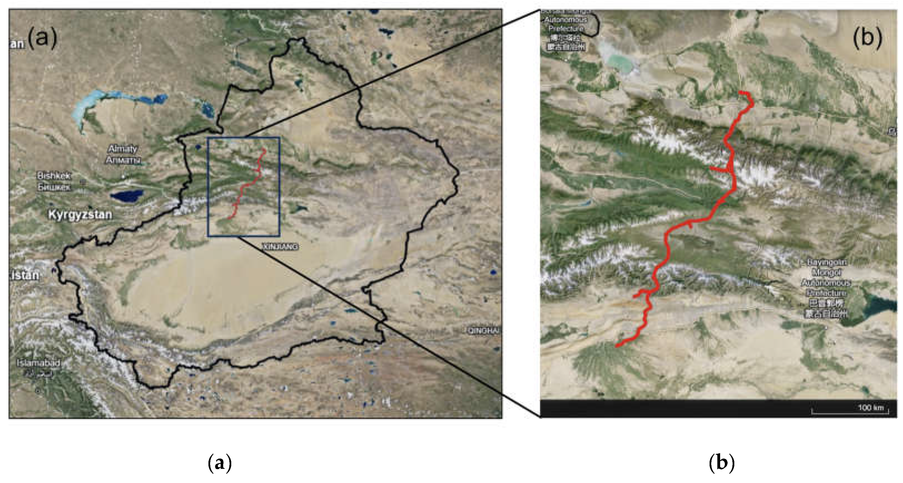
Figure 2.
Elevation of AOI.
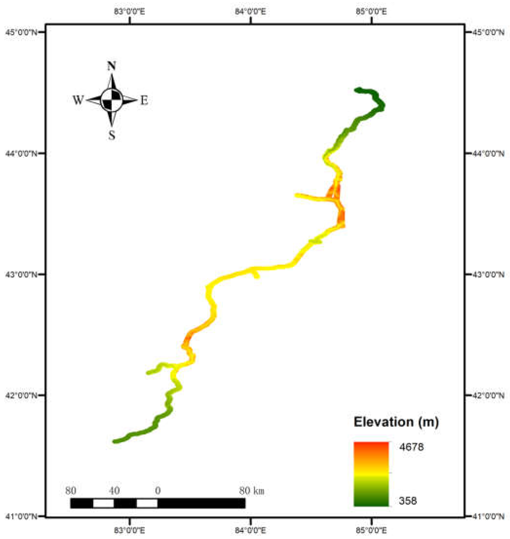
Figure 3.
Landslides identified during field survey.
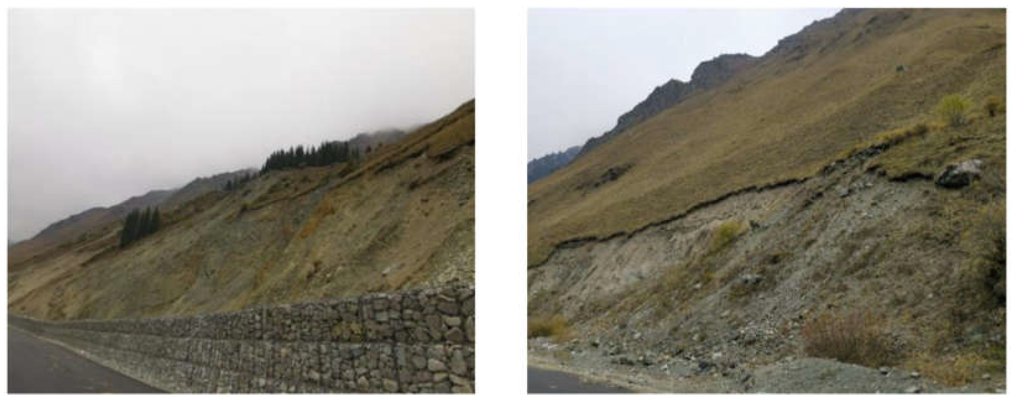
Figure 4.
Workflow of landslide susceptibility assessment along the G3033 Duku Expressway 2 km buffer zone.
Figure 4.
Workflow of landslide susceptibility assessment along the G3033 Duku Expressway 2 km buffer zone.
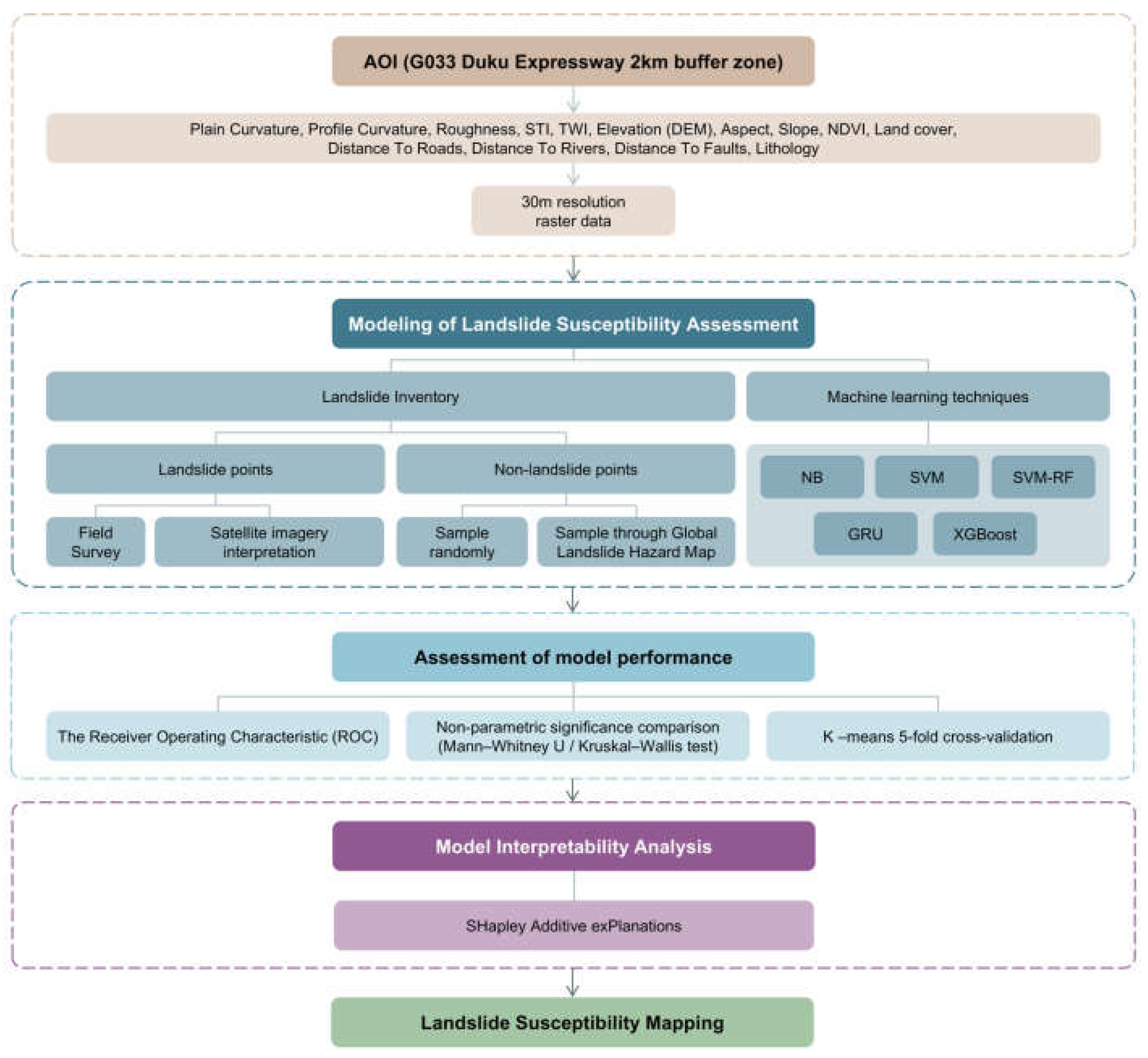
Figure 5.
Contributing factors for landslide susceptibility modeling represented as 30x30m raster images: (a) aspect; (b) elevation; (c) land cover; (d) distance to roads; (e) lithology; (f) NDVI; (g) plain curvature; (h) profile curvature; (i) roughness; (j) slope; (k) snowmelt; (l) STI; (m) TWI; (n) rainfall; (o) distance to rivers; (p) distance to faults.
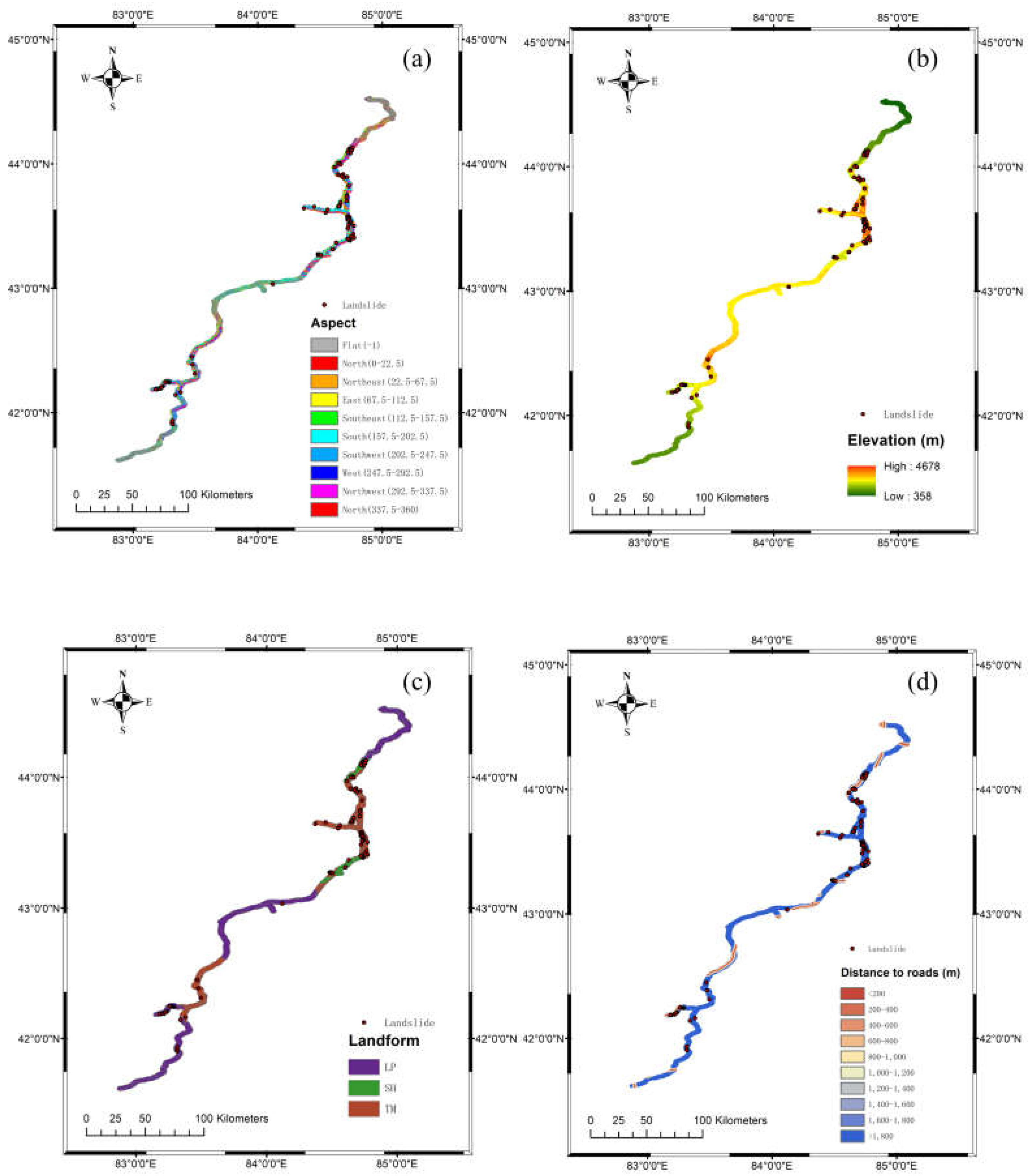
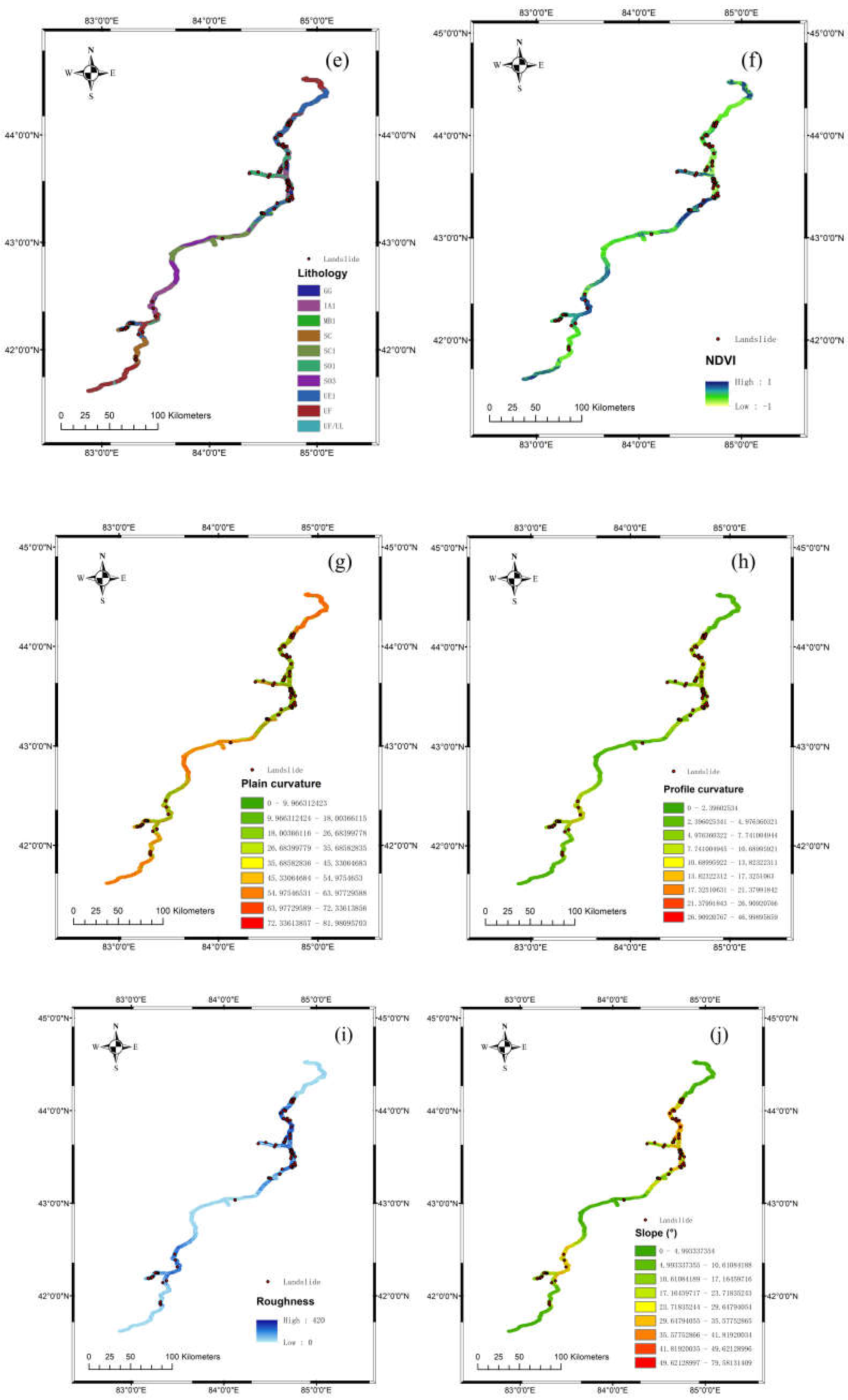
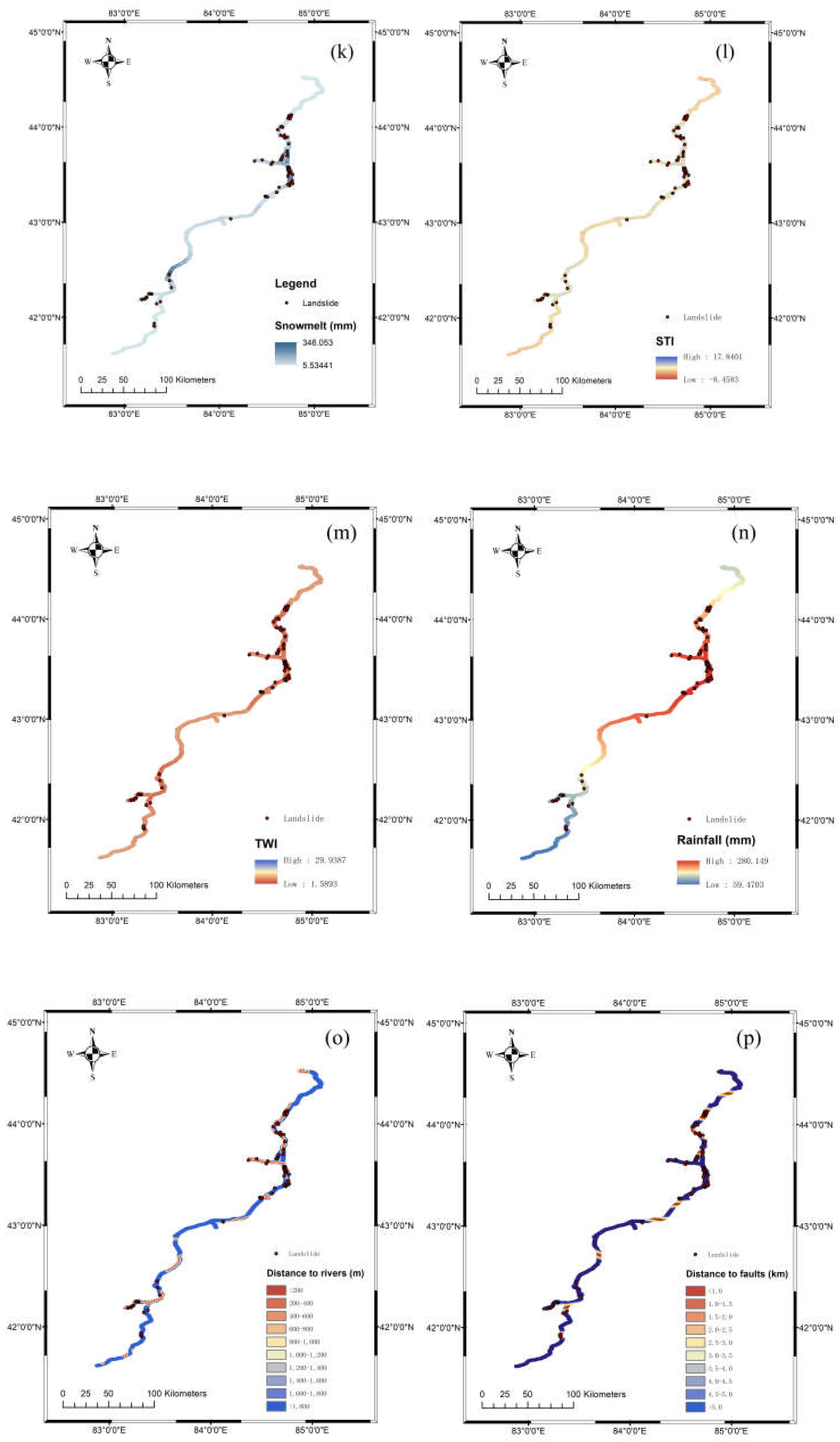
Figure 6.
The landslide inventory map displays both landslide points and non-landslide points. (On the left, non-landslide points are randomly sampled from the area of interest. On the right, non-landslide points are specifically selected from within the Low and Medium hazard levels as defined by The Global Landslide Hazard Map.).
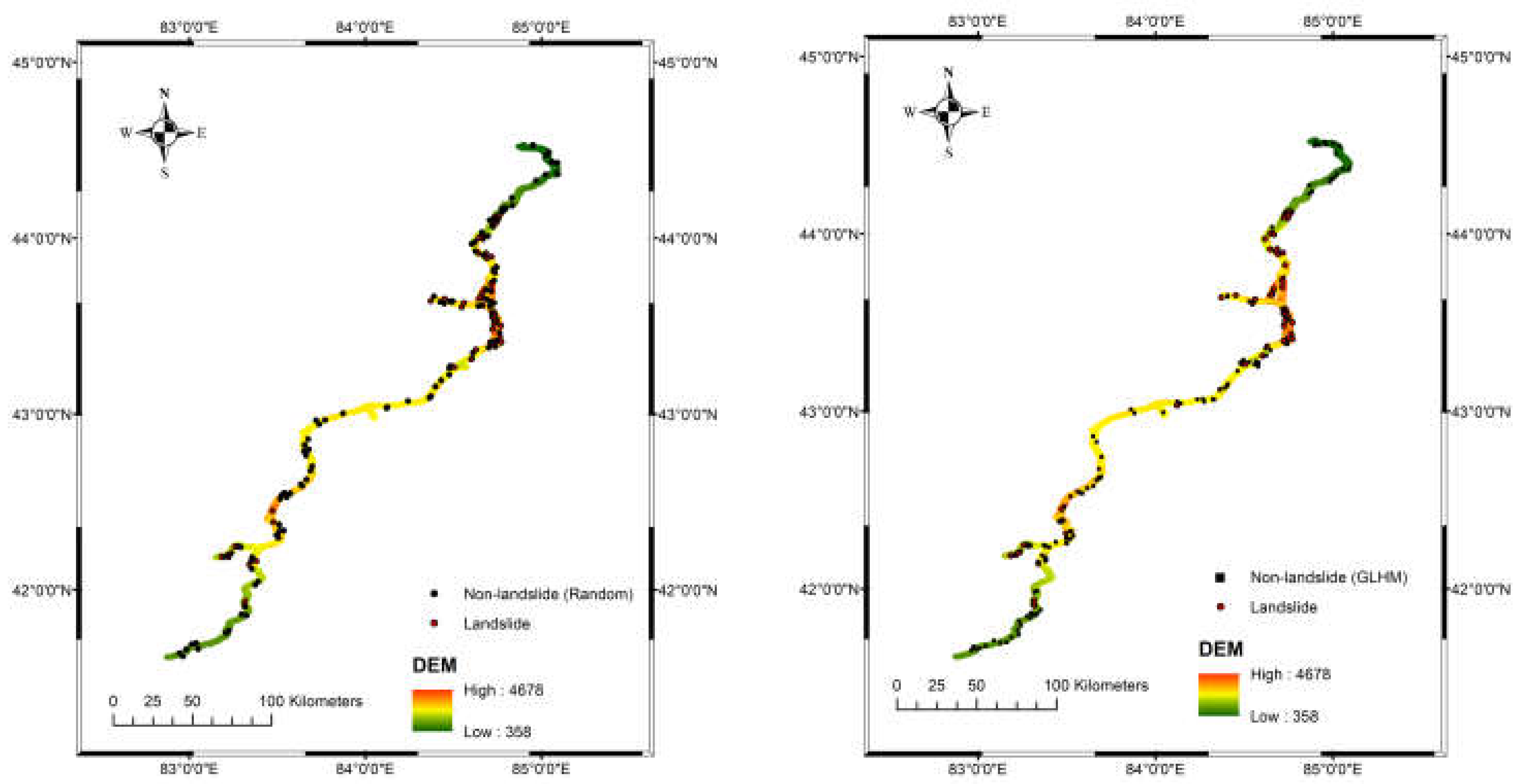
Figure 7.
Box plot comparing elevation distributions between Group 1 (Random method) and Group 2 (GLHM), two different methods for sampling non-landslide points.
Figure 7.
Box plot comparing elevation distributions between Group 1 (Random method) and Group 2 (GLHM), two different methods for sampling non-landslide points.
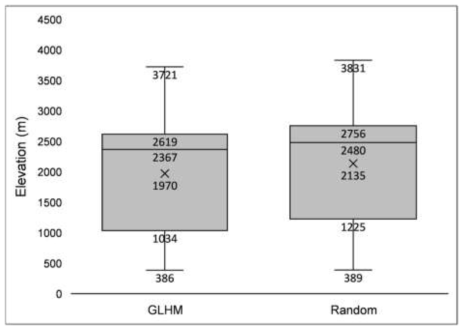
Figure 8.
Pearson correlation coefficients between each pair of 16 contributing indicators.
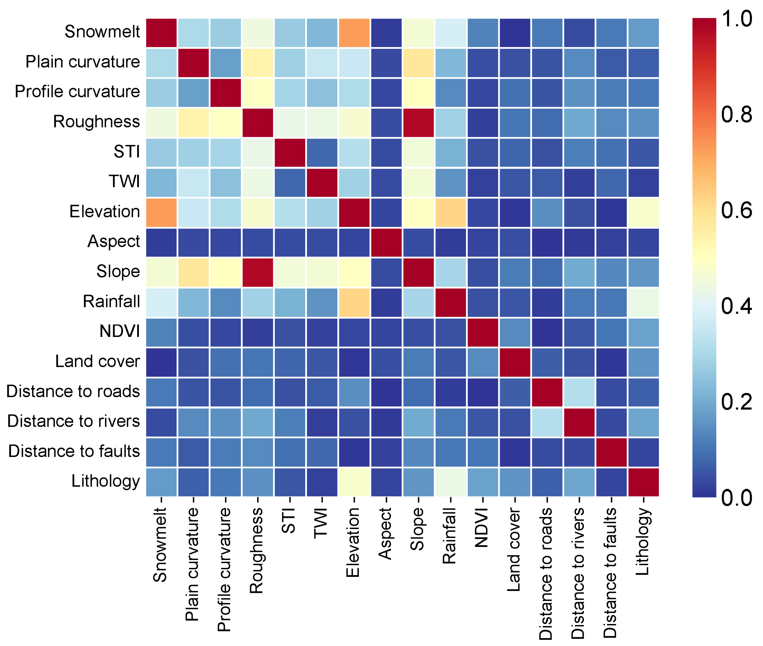
Figure 9.
Landslide susceptibility maps derived from: (a) NB-GLHM, (b) NB-Random; (c) SVM-GLHM, (d) SVM-Random; (e) SVM-RF-GLHM, (f) SVM-RF-Random; (g) XGBoost-GLHM, (h) XGBoost-Random.
Figure 9.
Landslide susceptibility maps derived from: (a) NB-GLHM, (b) NB-Random; (c) SVM-GLHM, (d) SVM-Random; (e) SVM-RF-GLHM, (f) SVM-RF-Random; (g) XGBoost-GLHM, (h) XGBoost-Random.
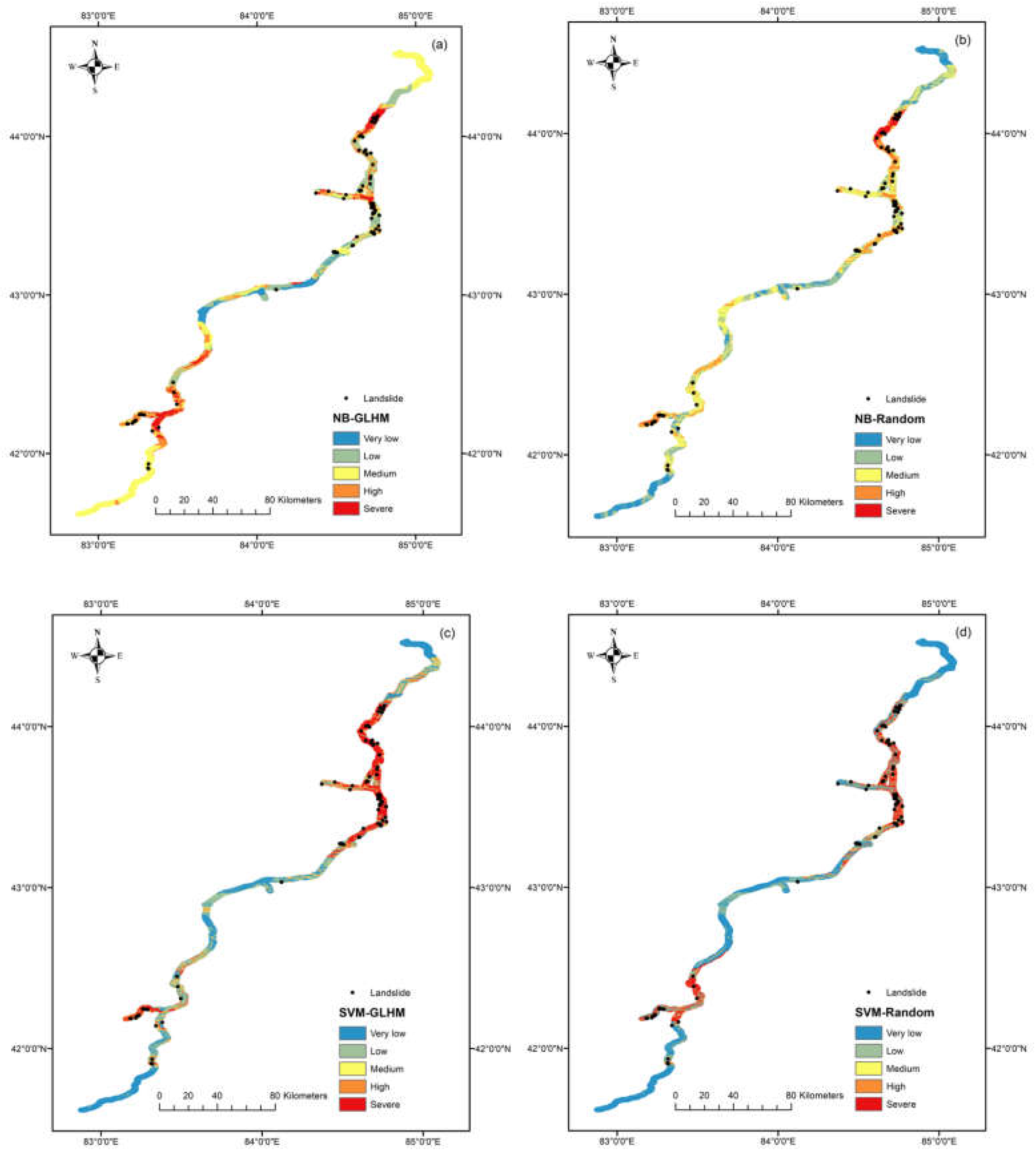
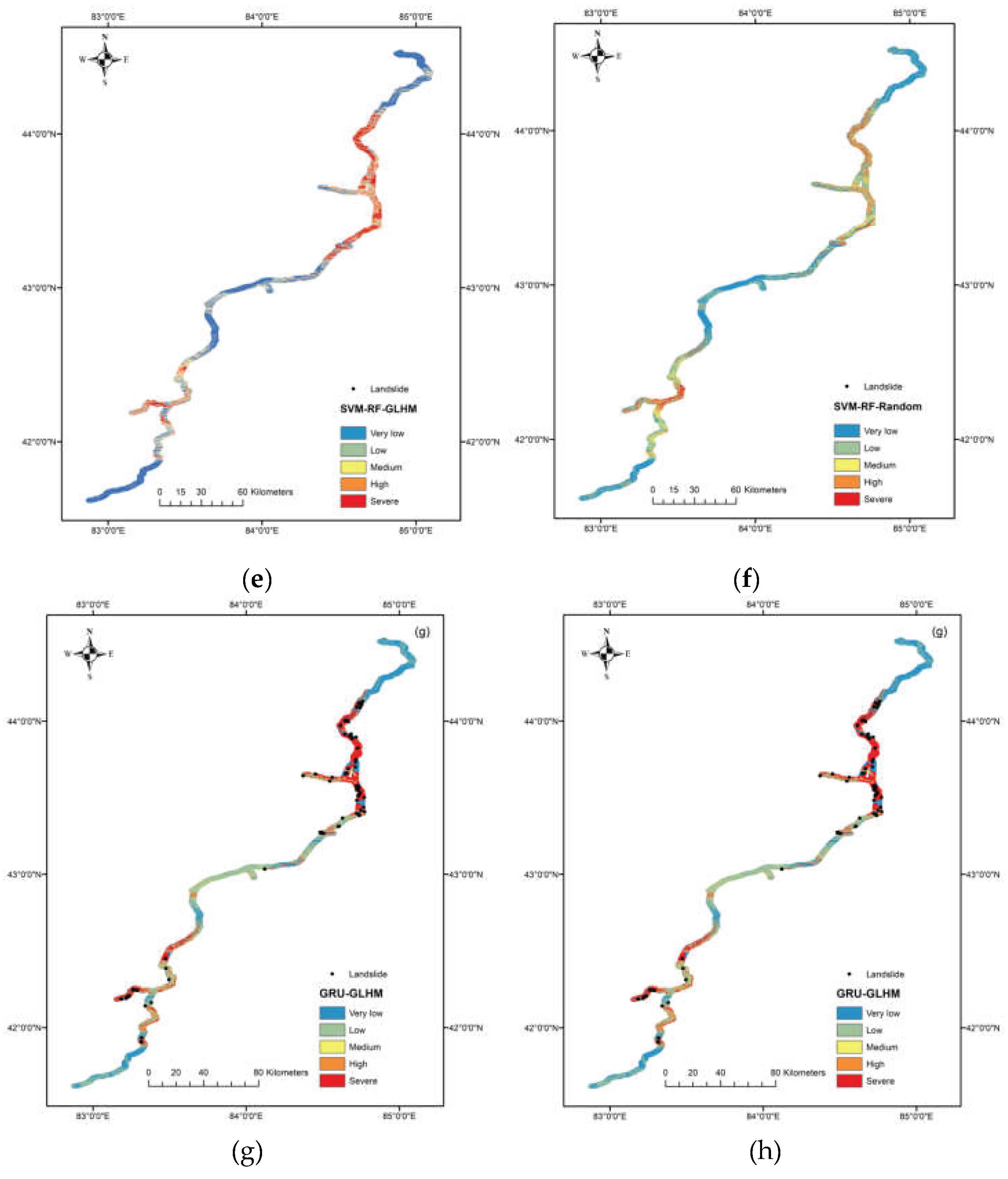
Figure 10.
ROC curves with AUC values.
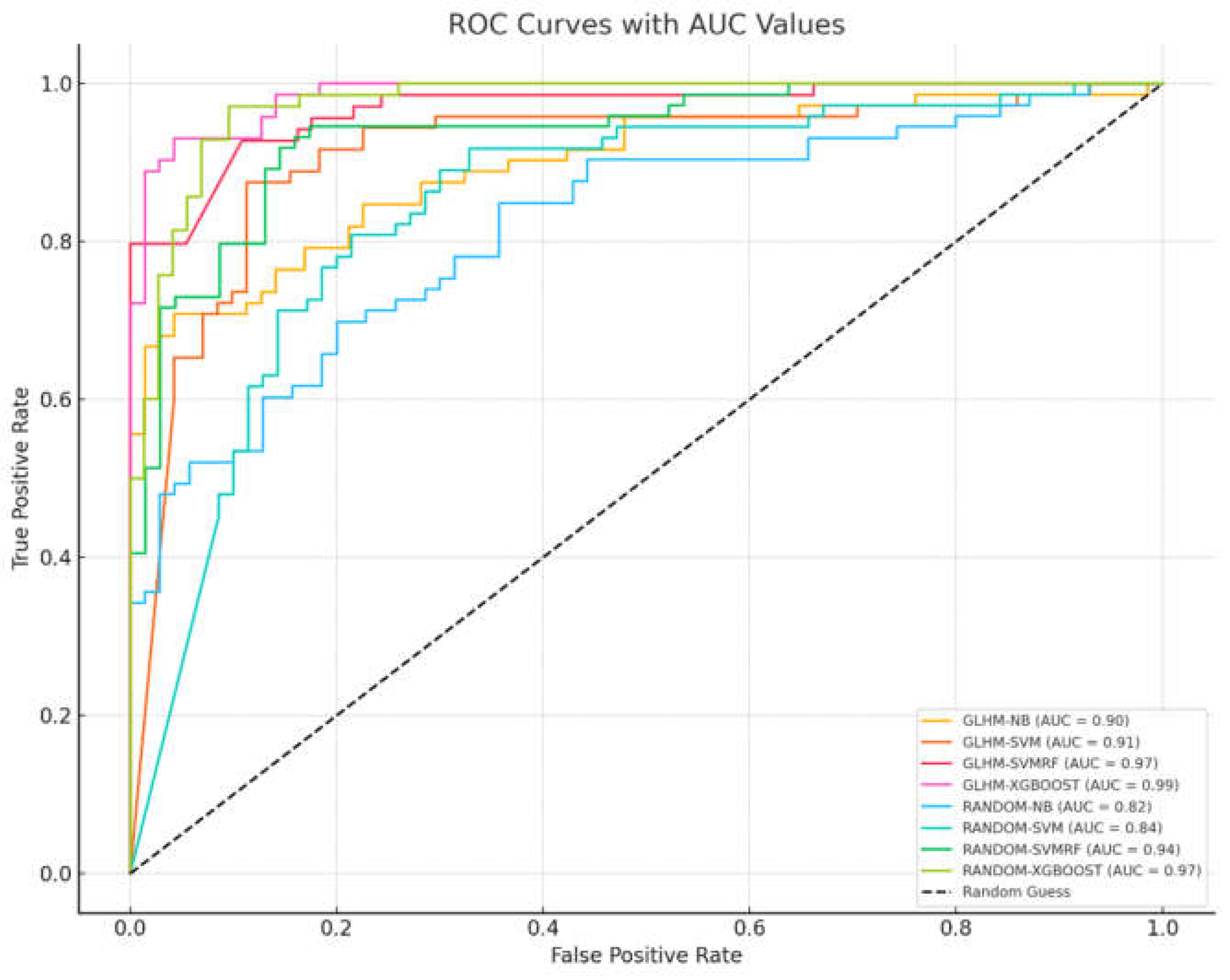
Figure 11.
Box-and-whisker plot of area under the receiver operating characteristic curve for landslide susceptibility models using different sampling methods for non-landslide points.
Figure 11.
Box-and-whisker plot of area under the receiver operating characteristic curve for landslide susceptibility models using different sampling methods for non-landslide points.
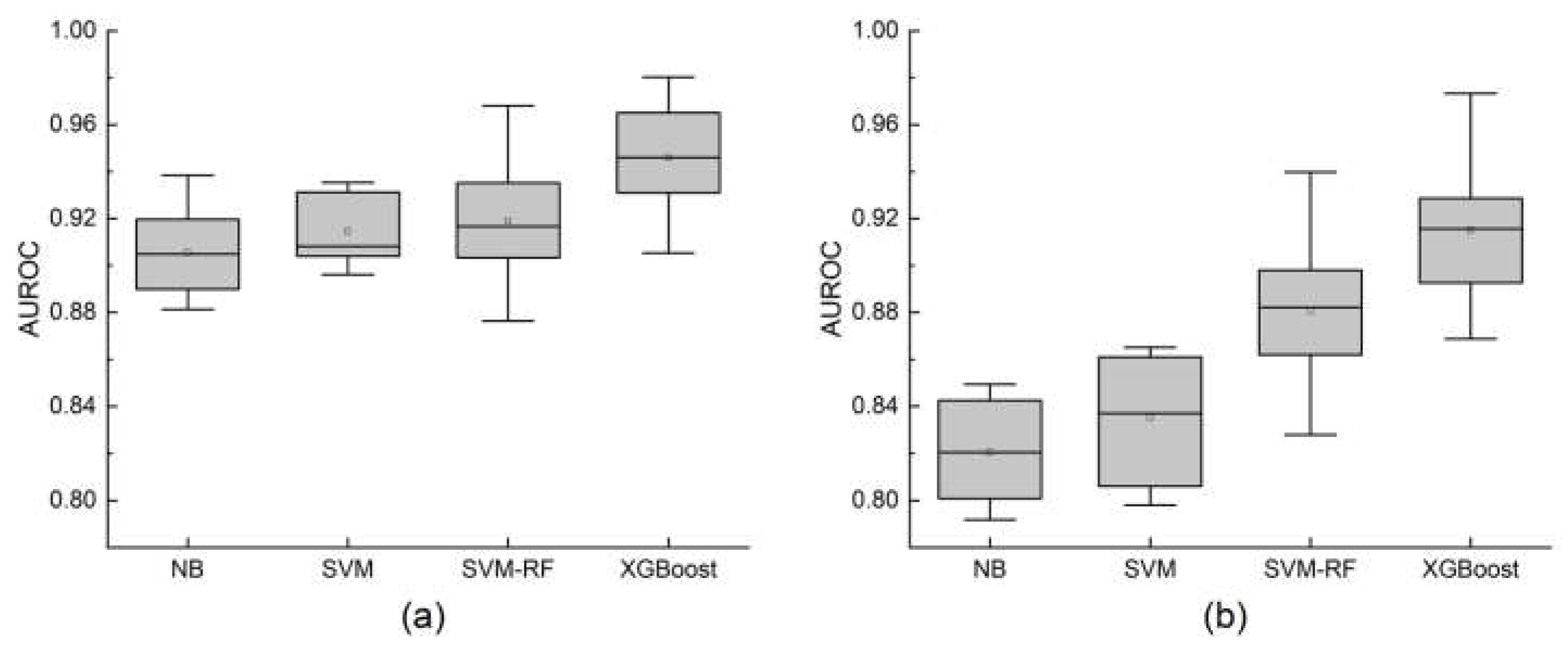
Figure 12.
Box-and-whisker plot of accuracy for landslide susceptibility models using different sampling methods for non-landslide points.
Figure 12.
Box-and-whisker plot of accuracy for landslide susceptibility models using different sampling methods for non-landslide points.
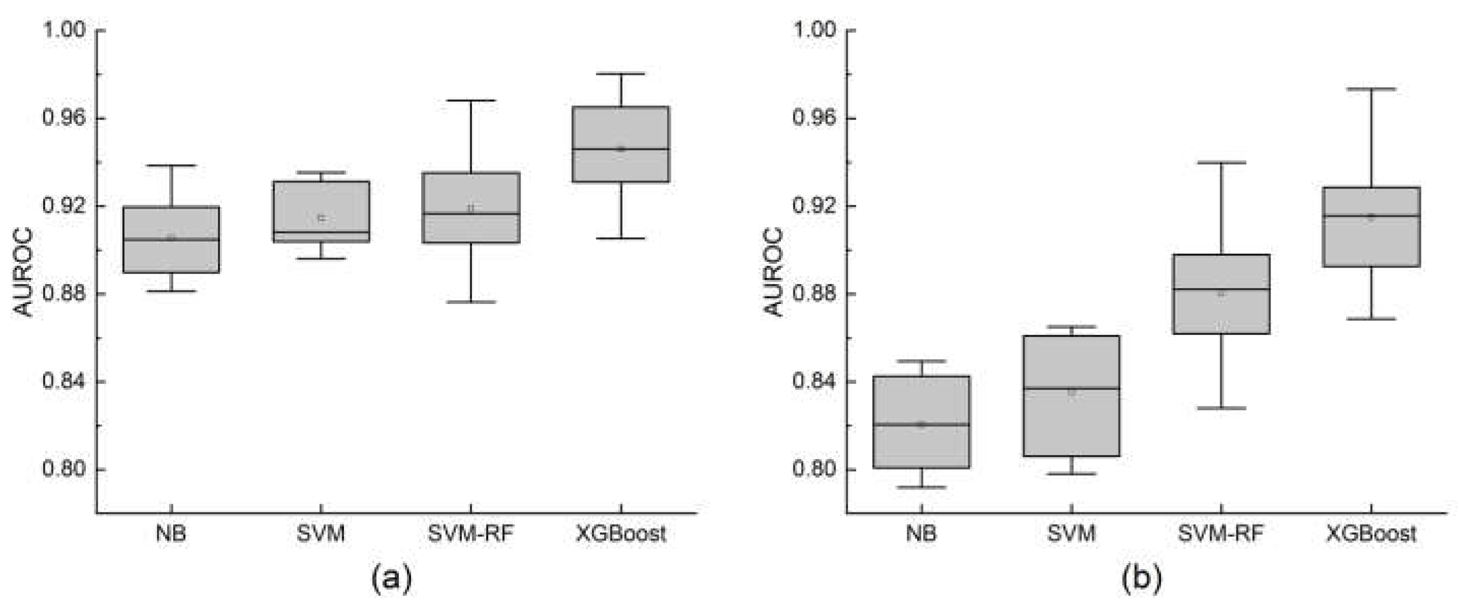
Figure 13.
Bi-modal violin plots of SHAP feature value distributions for five models — (a) NB, (b) SVM, (c) SVM-RF, (d) XGBoost — under two sampling methods: GLHM and random.
Figure 13.
Bi-modal violin plots of SHAP feature value distributions for five models — (a) NB, (b) SVM, (c) SVM-RF, (d) XGBoost — under two sampling methods: GLHM and random.
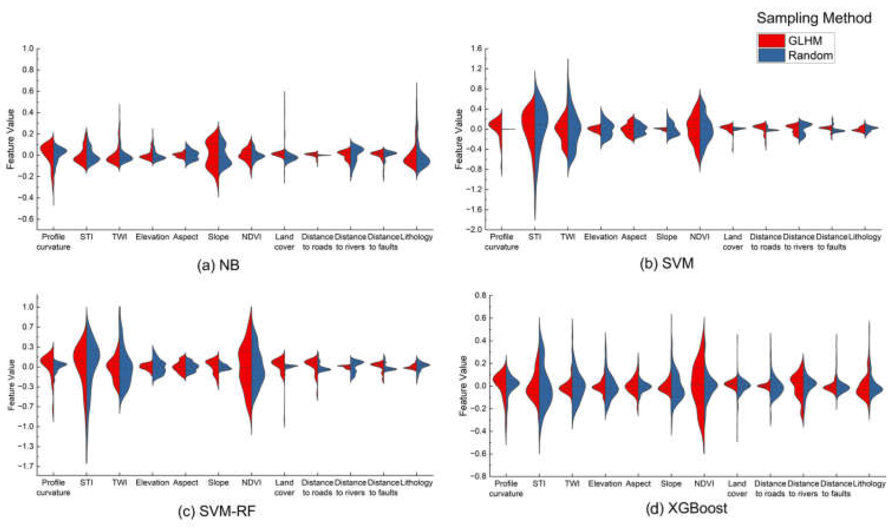

Table 1.
Contributing indicators used in multiple landslide susceptibility assessment studies.
| No. | Indicators system | Number of Indicators | Source |
| 1 | Elevation (m), Slope (°), Aspect, Slope length (m), Topographic wetness index (TWI), Plan curvature, Profile curvature, Distance from stream (m), Lithology, Distance from fault (m), Distance from geo-boundary (m), NDVI | 12 | Miloš, et al. [26] |
| 2 | Slope (°), Elevation (m), Plan curvature, Profile curvature, Catchment area, Catchment height, Convergence index, Topographic wetness index (TWI), Aspect, Surface roughness | 10 | Goetz, Brenning, Petschko and Leopold [12] |
| 3 | Elevation (m), Slope angle (°), Distance from lineaments (m), Forest type, Lithology, Soli drainage | 6 | Park [27] |
| 4 | Slope angle (°), Aspect, Elevation (m), Curvature, Plan curvature, Profile curvature, Soil type, Land cover, Rainfall (mm), Distance to roads (m), Road density (km/km2), Distance to rivers (m), River density (km/km2), Distance to lineaments (m), Lineament density (km/km2), | 14 | Binh Thai, et al. [28] |
| 5 | Slope (°), Aspect, Elevation (m), Plan curvature, STI, TWI, Distance to rivers (m), Distance to roads (m), Distance to faults (m), NDVI, Land use, Lithology, Rainfall (mm) | 13 | Chen, Peng, Hong, Shahabi, Pradhan, Liu, Zhu, Pei and Duan [19] |
| 6 | Slope (°), Elevation (m), Lithology, Distance to rivers (m), Relief amplitude (m), Rainfall (mm) | 6 | Meijun, et al. [29] |
Table 2.
Zonal statistics of landslide susceptibility maps.
| Model | Zoning | Area (km2) | Area Proportion | Number Of Landslide Points | Landslide Points Proportion | Landslide Points Density (point/km2) |
| NB-GLHM | Very low | 195.74 | 8.84% | 2 | 1.96% | 0.0102 |
| Low | 457.69 | 20.66% | 23 | 22.55% | 0.0503 | |
| Medium | 918.34 | 41.46% | 23 | 22.55% | 0.0250 | |
| High | 347.35 | 15.68% | 25 | 24.51% | 0.0720 | |
| Severe | 295.87 | 13.36% | 29 | 28.43% | 0.0980 | |
| NB-Random | Very low | 360.16 | 16.26% | 1 | 0.98% | 0.0028 |
| Low | 618.49 | 27.92% | 9 | 8.82% | 0.0146 | |
| Medium | 745.53 | 33.66% | 21 | 20.59% | 0.0282 | |
| High | 397.30 | 17.94% | 51 | 50.00% | 0.1284 | |
| Severe | 93.51 | 4.22% | 20 | 19.61% | 0.2139 | |
| SVM-GLHM | Very low | 771.69 | 34.84% | 1 | 0.98% | 0.0013 |
| Low | 396.21 | 17.89% | 3 | 2.94% | 0.0076 | |
| Medium | 252.14 | 11.38% | 2 | 1.96% | 0.0079 | |
| High | 252.83 | 11.41% | 5 | 4.90% | 0.0198 | |
| Severe | 542.13 | 24.48% | 91 | 89.22% | 0.1679 | |
| SVM-Random | Very low | 1170.48 | 52.84% | 2 | 1.96% | 0.0017 |
| Low | 263.89 | 11.91% | 2 | 1.96% | 0.0076 | |
| Medium | 181.34 | 8.19% | 4 | 3.92% | 0.0221 | |
| High | 191.23 | 8.63% | 12 | 11.76% | 0.0628 | |
| Severe | 408.05 | 18.42% | 82 | 80.39% | 0.2010 | |
| SVM-RF-GLHM | Very low | 836.32 | 37.76% | 1 | 0.98% | 0.0012 |
| Low | 408.70 | 18.45% | 6 | 5.88% | 0.0147 | |
| Medium | 329.52 | 14.88% | 17 | 16.67% | 0.0516 | |
| High | 350.06 | 15.80% | 26 | 25.49% | 0.0743 | |
| Severe | 290.40 | 13.11% | 52 | 50.98% | 0.1791 | |
| SVM-RF-Random | Very low | 934.45 | 42.19% | 7 | 6.86% | 0.0075 |
| Low | 589.61 | 26.62% | 18 | 17.65% | 0.0305 | |
| Medium | 358.73 | 16.20% | 40 | 39.22% | 0.1115 | |
| High | 181.34 | 8.19% | 14 | 13.73% | 0.0772 | |
| Severe | 150.86 | 6.81% | 23 | 22.55% | 0.1525 | |
| XGBoost-GLHM | Very low | 428.50 | 19.35% | 0 | 0.00% | 0.0000 |
| Low | 613.06 | 27.68% | 3 | 2.94% | 0.0049 | |
| Medium | 786.30 | 35.50% | 44 | 43.14% | 0.0560 | |
| High | 230.71 | 10.42% | 22 | 21.57% | 0.0954 | |
| Severe | 156.43 | 7.06% | 33 | 32.35% | 0.2110 | |
| XGBoost-Random | Very low | 407.70 | 18.41% | 5 | 4.90% | 0.0123 |
| Low | 534.19 | 24.12% | 6 | 5.88% | 0.0112 | |
| Medium | 873.28 | 39.43% | 33 | 32.35% | 0.0378 | |
| High | 251.73 | 11.36% | 32 | 31.37% | 0.1271 | |
| Severe | 148.11 | 6.69% | 26 | 25.49% | 0.1755 |
Table 3.
Model performance comparison across sampling strategies.
| Model |
GLHM Median (IQR) |
Random Median (IQR) |
Δ | p-Values |
| AUROC(%) | ||||
| NB | 90.49 (3.44) | 82.05 (4.29) | +8.44 | <0.001*** |
| SVM | 90.82 (2.93) | 83.71 (5.75) | +7.11 | <0.001*** |
| SVM-RF | 91.67 (2.83) | 88.22 (3.43) | +3.45 | 0.023 |
| XGBoost | 94.61 (3.58) | 91.56 (4.51) | +3.04 | 0.029 |
| Accuracy(%) | ||||
| NB | 82.62 (0.76) | 71.31 (2.68) | +11.30 | <0.001*** |
| SVM | 82.84 (1.84) | 74.51 (2.48) | +8.33 | <0.001*** |
| SVM-RF | 81.59 (2.13) | 74.20 (4.70) | +7.40 | 0.002** |
| XGBoost | 84.30 (2.81) | 75.99 (2.85) | +8.31 | <0.001*** |
| Significance code for adjusted p-values: p<0.001 “***”, p<0.01 “**”, p<0.05 “*”, p<0.1 “”, p>0.1 “ ”. | ||||
Table 4.
Statistical significance of pairwise model comparisons.
| Model pair | AUROC (%) | Model pair | Accuracy (%) | ||
| Significance | Adj. Significance (Bonferroni) | Significance | Adj. Significance (Bonferroni) | ||
| GLHM | |||||
| NB - SVM | 1.000 | 1.000 | SVM-RF - NB | 0.007 | 0.044 |
| NB - SVM-RF | 0.074 | 0.442 | SVM-RF - SVM | 0.074 | 0.442 |
| NB - XGBoost | 0.007 | 0.044* | SVM-RF - XGBoost | 0.007 | 0.044* |
| SVM - SVM-RF | 0.371 | 1.000 | NB - SVM | 0.371 | 1.000 |
| SVM - XGBoost | 0.074 | 0.442 | NB - XGBoost | 0.007 | 0.044* |
| Random | |||||
| NB - SVM | 0.074 | 0.442 | NB - SVM-RF | 0.371 | 1.000 |
| NB - SVM-RF | 0.007 | 0.044* | NB - SVM | <0.001 | <0.001*** |
| NB - XGBoost | <0.001 | <0.001*** | NB - XGBOOST | 0.007 | 0.044* |
| SVM - SVM-RF | 0.007 | 0.044* | SVM - RF-SVM | 1.000 | 1.000 |
| SVM - XGBoost | <0.001 | <0.001*** | SVM-RF - XGBOOST | 0.371 | 1.000 |
| SVM - RF-XGBoost | 0.371 | 1.000 | SVM - XGBOOST | 0.371 | 1.000 |
| Significance code for adjusted p-values: p<0.001 “***”, p<0.01 “**”, p<0.05 “*”, p<0.1 “”, p>0.1 “ ”. | |||||
Table 5.
Feature importance based on mean absolute SHAP values across models, with the top three features per model shown in bold.
Table 5.
Feature importance based on mean absolute SHAP values across models, with the top three features per model shown in bold.
| Contributing factors | Models | |||||||
| NB (GLHM) |
SVM (GLHM) |
SVM-RF (GLHM) |
XGBoost (GLHM) |
NB (Random) |
SVM (Random) |
SVM-RF (Random) |
XGBoost (Random) |
|
| NDVI | 0.0544 | 0.2358 | 0.3202 | 0.1715 | 0.0366 | 0.2268 | 0.2542 | 0.0822 |
| STI | 0.0649 | 0.2936 | 0.2947 | 0.1003 | 0.0573 | 0.3924 | 0.3447 | 0.1597 |
| TWI | 0.0541 | 0.2029 | 0.1646 | 0.0471 | 0.0471 | 0.3015 | 0.2455 | 0.1070 |
| Slope | 0.1374 | 0.0174 | 0.0962 | 0.0478 | 0.0832 | 0.1001 | 0.0363 | 0.1069 |
| Profile curvature | 0.0693 | 0.1517 | 0.1582 | 0.0922 | 0.0587 | 0.0005 | 0.0588 | 0.0671 |
| Distance to rivers | 0.0426 | 0.0704 | 0.0187 | 0.0911 | 0.0634 | 0.1008 | 0.0838 | 0.0643 |
| Lithology | 0.0674 | 0.0381 | 0.0283 | 0.0827 | 0.0902 | 0.0442 | 0.0605 | 0.0606 |
| Elevation | 0.0311 | 0.0383 | 0.0402 | 0.0448 | 0.0397 | 0.1260 | 0.0987 | 0.0880 |
| Aspect | 0.0103 | 0.0911 | 0.0714 | 0.0561 | 0.0376 | 0.0803 | 0.0610 | 0.0382 |
| Land cover | 0.0229 | 0.0613 | 0.1122 | 0.0366 | 0.0430 | 0.0212 | 0.0223 | 0.0436 |
| Distance to roads | 0.0140 | 0.0783 | 0.1078 | 0.0184 | 0.0021 | 0.0290 | 0.0596 | 0.0703 |
| Distance to faults | 0.0065 | 0.0413 | 0.0628 | 0.0343 | 0.0320 | 0.0527 | 0.0532 | 0.0428 |
Disclaimer/Publisher’s Note: The statements, opinions and data contained in all publications are solely those of the individual author(s) and contributor(s) and not of MDPI and/or the editor(s). MDPI and/or the editor(s) disclaim responsibility for any injury to people or property resulting from any ideas, methods, instructions or products referred to in the content. |
© 2025 by the authors. Licensee MDPI, Basel, Switzerland. This article is an open access article distributed under the terms and conditions of the Creative Commons Attribution (CC BY) license (https://creativecommons.org/licenses/by/4.0/).
Copyright: This open access article is published under a Creative Commons CC BY 4.0 license, which permit the free download, distribution, and reuse, provided that the author and preprint are cited in any reuse.


