
Submitted:
20 March 2025
Posted:
01 April 2025
You are already at the latest version
Abstract
Due to the lack of representativeness of standardized cycles such as the FTP-75, designed for specific regions and not adapted to cities such as Guayaquil, this study aimed to determine the representative driving cycles for the most congested urban routes of the city, covering the north, south, center and west zones. The methodology used was the direct method, carrying out trips in scenarios with real traffic. An M1 vehicle equipped with the OBDLINK MX+ device was used, which allowed data collection in real time. These data were processed and analyzed with the OBDWIZ program to characterize local driving patterns. With the support of the Minitab tool, the sample size was determined from the data obtained in the pilot tests performed on each route. In addition, normality tests were performed on each route to determine the distribution of the data and apply the most appropriate measure of central tendency. Finally, using the weighting criteria method, the representative cycle for each route was determined. The results obtained showed that, on Route 1, the selected repetition was 7, with an average speed of 65.39 km/h and a maximum speed of 79 km/h. For Route 2, repetition 11 was selected, with an average speed of 21.39 km/h and a maximum speed of 67 km/h. For Route 3, the chosen repetition was 2, with an average speed of 11.05 km/h and a maximum speed of 50 km/h. Finally, for Route 4, the selected repetition was 5, with an average speed of 16.27 km/h and a maximum of 39 km/h.
Keywords:
driving cycle
; urban routes
; traffic congestion
1. Introduction
Traffic congestion in urban areas, such as Guayaquil and its environment, represents a significant problem in terms of mobility and environmental impact. Excessive traffic affects travel efficiency and contributes to polluting gas emissions, deteriorating air quality and posing risks to public health [1]. Internal combustion engines release substances such as carbon monoxide (CO), carbon dioxide (CO2), nitrogen oxides (NOx), unburned hydrocarbon (HC) and lead compounds [2]. According to the World Meteorological Organization, between 1990 and 2022 greenhouse gas emissions increased by 49 percent, with CO2 beingresponsible for 78 percent of this increase [3,4].
In order to decrease the environmental impact of the transportation sector, numerous studies have been developed, and governments have implemented strict regulations to control emissions, including a representative driving cycle (DC) [5]. China adopts this initiative by replacing the European Driving Cycle (NEDC) with the Driving Cycle (WLTC) [6], which is based on emissions tests under real driving conditions (RDE) [7]. However, although this globally standardized and harmonized cycle works well at altitudes below 2400 masl, it is not suitable for higher altitudes. A detailed study reveals that, at these 35 altitudes, engine efficiency decreases and traffic in high density areas aggravates the problem [8,9].
A study in Mexico oriented to the evaluation of pollutant emissions in freight vehicles highlights a comparison between a DC performed by them and other international reference cycles applied in that country, which results show that, in relation to simulated emissions, problems were observed when adopting international DCs. The results show that, incomparison with the DC determined in the study area, emissions can be underestimated by 19 percent for NOx and 25 percent for CO if the EPA Federal Test Procedure (FTP-75) [10] is adopted; this is due to the fact that the DC chosen will not have the same driving patterns or the same topology as the place where the tests would be carried out [11].
In several countries, DCs are developed to reflect local driving conditions [12], whether legislative or not [13], because they want to obtain more accurate data in their studies. In the United States, Japan and the European Community established legislative cycles such as FTP-75, NEDC and JC08, respectively, to meet vehicle emission regulations [3].Non-legislative cycles have been analyzed in cities such as Vadodara, Bangalore, Hong Kong, Pune, Edinburgh, Athens, Singapore, 11 Chinese cities and Malaysia with its MUDC.These are used for energy, efficiency and emissions studies, as well as in certifications and laboratory tests [14,15].
On the other hand, studies carried out in several cities in Ecuador, such as Esmeraldas, Ambato, Cuenca, among others, detailed the importance of these investigations. This was due to the fact that, by implementing a representative cycle for these specific regions, better results can be obtained in the evaluation of fuel consumption and emissions. The methodology used for data collection was the direct method, which consisted of obtaining information in real time using the ON BOARD technique. For this purpose, the vehicle was equipped with an OBD or GPS device and two or more drivers were involved in order to simulate the best traffic conditions. Finally, the method used to obtain the representative driving cycle was based on the weighting criterion, which assigned a relative weight to each of the selected variables, reflecting their importance in the characterization of the driving cycle. Thus, through the equation of weighted averages, the optimal route was determined, ensuring that it accurately reflected the actual driving conditions in the area. [16,17,18].
In consideration, this study aims to determine the DC in urban routes in the city of Guayaquil, analyze the traffic behavior of specific routes where a series of data will be collected to obtain the actual driving pattern in the selected routes, using as a tool an OBD LINK MX+ device. These data were implemented for a statistical analysis, where the normality test was determined for each route to determine the distribution of their data. Finally, using the weighting criteria method, the selected repetition was determined for each route, which corresponds to its respective driving cycle.
This study, carried out at the Polytechnic Salesiana University of Ecuador (UPS) Guayaquil, during the period 2024 - 2025, is directed not only to the academic community, providing theoretical foundations for future research, as well as municipalities and other entities interested in the DC. It also represents a novel approach to evaluate various parameters under different conditions, through the implementation of a methodology, taking as references the standardized cycles. The expected results seek to provide valuable information to understand the real dynamics of traffic and its environmental impact in the urban environment of Guayaquil.
The lack of specific DC adapted to local conditions represents a challenge in vehicle design, energy consumption assessment and pollutant emission control in vehicle homologation processes [19]. Although an ideal DC should reflect the common driving style under different traffic conditions, considering key factors such as vehicle technology, traffic 85 characteristics, and climatic and geographical conditions (such as altitude), in many cases an adequate representation is not achieved. In Ecuador, the National Traffic Agency (ANT) and the Ecuadorian Standardization Service (INEN) are responsible for implementing these cycles for vehicle certification [20], where the ideal time for a DC is 25 minutes according to research conducted by Giraldo in 2021 [21].
Previous studies highlight the importance of developing a representative DC that adapts to local characteristics, allowing a more accurate evaluation of vehicle performance under real operating conditions and optimizing its adaptation to the topology and urban traffic of the region. In Guayaquil, the absence of a specific DC represents a major challenge, since foreign cycles, such as the FTP-75 [22,23], are currently used. This generates significant discrepancies, since these cycles do not adequately reflect the driving patterns typical of the geographical environment and the real conditions of the city.
2. Materials and Methods
2.1. Description of the Study Area
This study was conducted in the city of Guayaquil, located in the coastal region of Ecuador. It is the most populated city in the country, with more than 2.7 million inhabitants, which represents 16 percent of the national population, according to data from the 2022 census [24]. It has a territory of approximately 380 square kilometers and an average altitude of 4 meters above sea level. Its climate is tropical, with high temperatures throughout the year.
For the reliability of the data obtained, specific routes were selected within the urban area of Guayaquil, covering the northern, southern, western and central areas with the highest traffic congestion. These routes were defined in strategic areas that reflect the real and usual driving conditions, characterized by a high level of traffic, thus establishing a total of four main routes.
For the selection of routes, several criteria must be taken into account:
- A large flow of vehicles;
- Linking the main population centers;
- Numerous squares and crossroads;
- Access to public transport networks, for the purpose of normal driving [25].
Juan Tanca Marengo Avenue is one of Guayaquil’s main thoroughfares, connecting several key sectors of the city. This avenue extends from the north, in areas near Rodrigo Chávez González Avenue, to the Maritime Port sector, and passes through high-density commercial and residential areas. Due to its strategic location, it is a road with a high vehicular flow, used by both public and private transportation, which makes it a neuralgic point for urban mobility. In addition, the avenue is home to a large number of stores, restaurants and services, which reinforces its economic importance [26].
The last accountability report for the year 2023 presented by the Agencias de Tránsito y Movilidad (ATM) [27] streets such as Av Portete located in the southern area of Guayaquil is a busy road that connects several important roads and passes through residential areas with small businesses, markets and public transport stations, and is characterized by high pedestrian and vehicular activity. Machala Street, on the other hand, located in the south-central area of the city, is characterized by its dense commercial and labor activity, houses workshops, retail stores and connects with important streets leading to the city center and surrounding areas. Finally, Via a la Costa is one of the city’s main thoroughfares, designed for fast vehicular traffic, connecting Guayaquil with neighboring cities and tourist destinations along this road, where there are private housing developments, shopping centers, schools and housing developments to consolidate as a city.
The main points of vehicular traffic in different streets of the city were identified with the support of the GPS navigation platform Google Maps, a tool that allows analyzing daily traffic in certain places. In addition, Diario El Universo [28] in its study used this platform along with interviews to provide results in the most conflictive areas of the north, west, south and center of the city. This information helped to determine 4 specific routes for the analysis.
Route 1, illustrated in Figure 1 (a), covers a total distance of 14.9 kilometers. The route begins on Via a la Costa, near the crosswalk that connects to the Puerto Azul housin development. From this point, the route continues along Vía a la Costa, characterized by its wide roadway and constant flow of vehicles, until reaching the entrance to the Chongón toll booth, located on the border between urban developments and areas of transition to rural and recreational zones. According to the Escuela Superior Politécnica del Litoral (ESPOL), the Via a la Costa sector is considered an urban area within the city, which concentrates 23.14 percent of the urban land [29,30].
Route 2, shown in Figure 1 (b), has a total length of 5.7 kilometers and covers an urban route that connects several key points in the city. The route begins at the San Marino shopping center. From there, it moves towards Avenida Rodrigo Chávez, a main artery that connects important sectors of the city. Along this avenue, the route continues until reaching Juan Tanca Marengo Avenue, another important road that crosses the city in an east-west direction. Finally, the route concludes at the Colegio Americano facilities.
Route 3, shown in Figure 2 (a), is 4.7 kilometers long and covers an urban route that connects strategic points in the city. The route begins at the Centenario campus of the UPS (Universidad Politécnica Salesiana del Ecuador). From there, the route follows a series of streets until it reaches Portete Street and 17th Street, in front of a well-known KFC fast foodrestaurant, an easily recognizable place in the area. This route was selected especially for its relevance in terms of traffic density and flow, making it a key route for urban commuting.
Route 4, shown in Figure 2 (b), has a total distance of 3.9 kilometers and runs through aspecific sector within the city, connecting several main avenues. The route begins at Avenida 9 de Octubre, one of the most important and busiest arteries, known for its commercialactivity and access to several key points in the city. From there, the route continues alongAvenida Francisco Aguirre Abad, a road that also has relevance in urban connectivity and vehicular flow. Subsequently, the route advances along Machala Avenue, a street that crosses different residential and commercial areas, and finally concludes on El Oro Street, another significant point within the city’s road network.
2.2. Vehicle Selection
2.3. Measuring Instruments and Data Collection
The “OBDLINK MX” diagnostic device was used as a tool to collect speed data. It is connected to the vehicle’s OBD II port, which is usually located on the lower part of the dashboard, near the steering wheel. This port allows communication between the device and the different control units of the vehicle, facilitating the diagnosis of problems and the reading of data [32].
It is important to note that the use of this device for data collection involves the application of several protocols, being in this case supported by ISO 15765-4:2016. This standard focuses on diagnostic communication via the controller area network (CAN) in vehicles, which ensures greater reliability and more accurate data collection [33].
The device was operated using the “OBDWiz” program, an application designed for Windows systems. This tool made it possible to interact with the vehicle’s ECM (Engine Control Unit) through an intuitive interface and a firm structure. Thanks to this, real-time data can be obtained and key parameters related to the vehicle’s performance and general condition can be analyzed, thus extending its capabilities for automotive diagnostics. In addition, it was necessary to use a voltage converter to ensure that the computer with the installed software remained charged during data collection.
Finally, the application used for traffic analysis was Google Maps, an effective tool for mobility and traffic analysis. It provides real-time data on congestion, travel times and traffic patterns. Thanks to its detailed information and up-to-date databases, it facilitates road efficiency analysis, optimal route planning and customization of studies through Google My Maps and its traffic management APIs [34].
2.4. Data Collection Methodology
The methodology used in this study is the so-called direct method, which consists in the acquisition of data of speed values with respect to the time of the real conditions of urban traffic in the city, a clear example is the American cycle FTP 75, which is used in the homologation and consumption tests in Ecuadorian vehicles. By means of this method, data collection can be obtained by different techniques, of which the ON BOARD technique was used, which consists of the instrumentation of the vehicle, in which a category M1 vehicle was used. At the same time, 3 drivers were required, alternating on each route, to simulate the real conditions on the routes [16,17].
The Chevrolet Aveo Emotion 1.6 4P 4X2 TM, which was instrumented with an OBD device, was used as the test vehicle. The OBDLINK MX+ was used to collect data in real time, along with the OBDWiz program for processing and storing data on each of the runs. The input variables recorded in the program are: speed, time, distance, as the main parameters for the elaboration of the characteristic curves.
Pilot tests were conducted for the selection of the routes established in various areas of the city of Guayaquil, comprising the North, South, Center and West; in which the total number of repetitions was established for each route. Next, in Figure 3 (a), a flow chart was made that explains in detail the process used to acquire data and obtain the representative DC for each route: first, the vehicle was turned on and the presence of any warning indicator on the dashboard was verified. If any anomaly was detected, the vehicle was taken to a workshop for diagnosis. In the absence of warnings, the fuel, oil and coolant levels were checked to ensure that the vehicle was in optimum condition.
Then, the route was chosen and, in turn, the vehicle was instrumented using the OBD LINK MX+ device. Then, the OBDWiz program was opened to record the input variables, and the software started to collect the information during the trip. Once finished, the data recording was stopped, and the data was imported in “.csv” format in Microsoft Excel. Finally, the data was collected, and, through statistical analysis, normality tests were determined for each route using Minitab software, in order to analyze the distribution of the data and obtain DC for each one. For the correct instrumentation and monitoring of data in the vehicle, it was essential to follow a specific procedure for each established route, as shown in Figure 3, item (b).
2.5. Data Analysis Methods and Techniques
2.5.1. Data Analysis Tools
The specialized statistical analysis software Minitab was used, which is a tool recognized for its ability to investigate and analyze data in different areas. It provides a platformthat allows users to perform exploratory data analysis, hypothesis testing, statistical modeling and quality control with high scientific accuracy. Its user-friendly interface and diverse statistical functionalities facilitate the conduct of studies and drive data-driven decision making in both academia and industry [35,36].
2.5.2. Data Analysis Methodology
The following variables were collected and used in different studies to obtain a representative driving cycle [16,18]:

Table 2.
Variables of analysis.
| Variables of analysis |
|---|
| Controllable variables |
| Distance (km) Time (s) |
| Non-controllable variables |
| Ambient temperature (Celsius) Altitude (m.s.n.m.) Wind speed (m/s) Fuel quality (Octane) Route conditions (Regular) |
| Response variable |
| Maximum speed (km/h) Average speed (km/h) Number of stops (N) Idle time (s) Positive acceleration time (s) % of driving time % of time accelerating |
2.5.3. Data Processing Methodology
The methodology implemented for the analysis of the data obtained was based on previous studies carried out in different countries, such as the United States, Colombia, among others [37]. Likewise, it was used in the determination of driving cycles in various cities of Ecuador, such as Quito, Esmeraldas, Cuenca and Riobamba [16,17,18,38], applying the weighting criterion. This method consisted of selecting, within a set of data, the most relevant one. To this end, each variable was assigned a value according to its degree of importance, using a scale from 0 to 1, where 0 represented the least importance and 1 the greatest. These values were established in multiples of 0.25. Table 3 shows the weighting weights assigned to each variable previously defined, according to its relevance.
Next, the lowest value of “Y” is selected because it represents the smallest deviation from the mean/median. This is determined as follows:
- Y: Weighted mean/median of the deviations of all parameters from the arithmetic mean.
- Wi: Weighting coefficient.
- X(i,j): Value of the variable.
- : Mean / median of the variable.
- : Deviation from the mean/median with absolute value.
It is worth mentioning that, before performing this analysis, it is necessary to carry out a normality test to determine the distribution of the data. From there, the centra tendency measure is calculated, which can be the mean or the median. Then, the weighted mean/median of the deviations of all variables from the arithmetic mean “Y” is calculated for each of the cases, as in Equation 1. Finally, the minimum value of the total obtained is selected. This value represents the smallest deviation from the mean/median, which indicates that the driving cycle among the analyzed repetitions corresponds to the one with the smallest value of “Y”.
3. Results
3.1. Pilot Test
Pilot tests were carried out to determine the routes in different areas of the city of Guayaquil, establishing a total of four routes as shown in Table 4. To calculate the sample size, Minitab software was used to determine the total number of repetitions for each route. Prior to this calculation, a descriptive analysis was carried out in Minitab, through which the deviation and standard error of the mean were obtained, fundamental elements for establishing the sample size. The variable that was analyzed was speed, given that, since we are dealing with driving cycles, the main parameters of this study were speed and time.
From the data collected in each pilot test, the standard deviation and standard error were calculated to estimate the appropriate sample size for each route. This analysis was performed using Minitab software, which allowed determining a total of 12 replicates for Route 1 and 11 replicates for the other routes, as detailed in Table 5. In total, 45 replicates were obtained.
3.2. Data Collection
After completing all the repetitions, the processing of the data stored in the Microsoft Excel program was started, in which the data from each of the repetitions were grouped in their respective route, including the pilot tests. Once the data were collected and organized, filtering began with a resolution of 1 second. This is because the results obtained for each repetition were recorded at 0.1 second intervals, generating a total of 10,000 data per repetition.
The reduction in resolution was essential to eliminate visual noise and highlight major trends, allowing for a less dense graphical representation while maintaining meaningful patterns. This adjustment simplified the plots, preserving the overall trends more clearly [39,40,41]. In addition, this process reduced the data for each repetition from 10,000 to a range of 700 to 1000 data per repetition, making it easier to manipulate and analyze. Once the data were pooled and filtered, normality tests (N.P.) were performed for each of the routes to determine the distribution of the data and select the appropriate measure of central tendency [42].
3.3. Analysis of Data Obtained
The data obtained for Route 1 (Via a la Costa-Peaje), which included 12 repetitions, are presented below. In each repetition, the OBD LINK MX+ device was used to record the variables detailed in Table 6. These variables reflect traffic behavior and are fundamental for obtaining and analyzing the driving cycle.
For Route 2 (San Marino - Colegio Americano), which included 11 replicates, the variables listed in Table 7 were recorded.
Likewise, for Route 3 (Av. 9 de Octubre - El Oro), which included 11 repetitions, thevariables listed Table 8 were recorded.
Finally, for Route 4, comprising UPS Centenario - 17th Street and Portete, data were 300 collected for its 11 repetitions, on various variables, which were recorded directly by the 301 OBD device, as shown in Table 9.
3.4. Normality Test
Once all the routes had been compiled, the statistical analysis of this study was carried out. As part of the analysis, it was necessary to examine the distribution of the data obtained. Appendix B presents the Anderson-Darling normality test, which was applied to each of the routes evaluated in the experiment. On the other hand, to carry out this analysis, the data corresponding to the repetitions performed for each route were grouped in order to obtain the specific normality test in each case.
Using Minitab software, the Anderson-Darling normality test was run on the four routes analyzed, since this test allows one to verify whether the data follow a normal distribution. Figure 4 (a) shows the test applied to route 1 (Via a la Costa-Peaje). The results indicate that the data are not normally distributed, as the obtained value of p is less than 0.05, which leads to the rejection of the null hypothesis. Therefore, the median is used as a representative measure for this route.
Similarly, the tests applied to the other routes, shown in Figure 4(b), (c) and (d), also reveal that the data do not follow a normal distribution. Consequently, the same median-based method was used for the remaining routes.
3.5. Weighting Criteria
After performing the normality test, it was determined that the data did not follow a normal distribution. For this reason, the median (X) was calculated from the 12 repetitions. With these values, the “Y” value was obtained for each of the variables analyzed in each of the repetitions of Route 1 (Via a la Costa - Toll). Subsequently, these values were added in each repetition to obtain the total “Y” in each case. Finally, the value with the smallest deviation with respect to the median was selected, thus identifying that the corresponding driving cycle among the selected repetitions is number 7, as shown in Table 10.
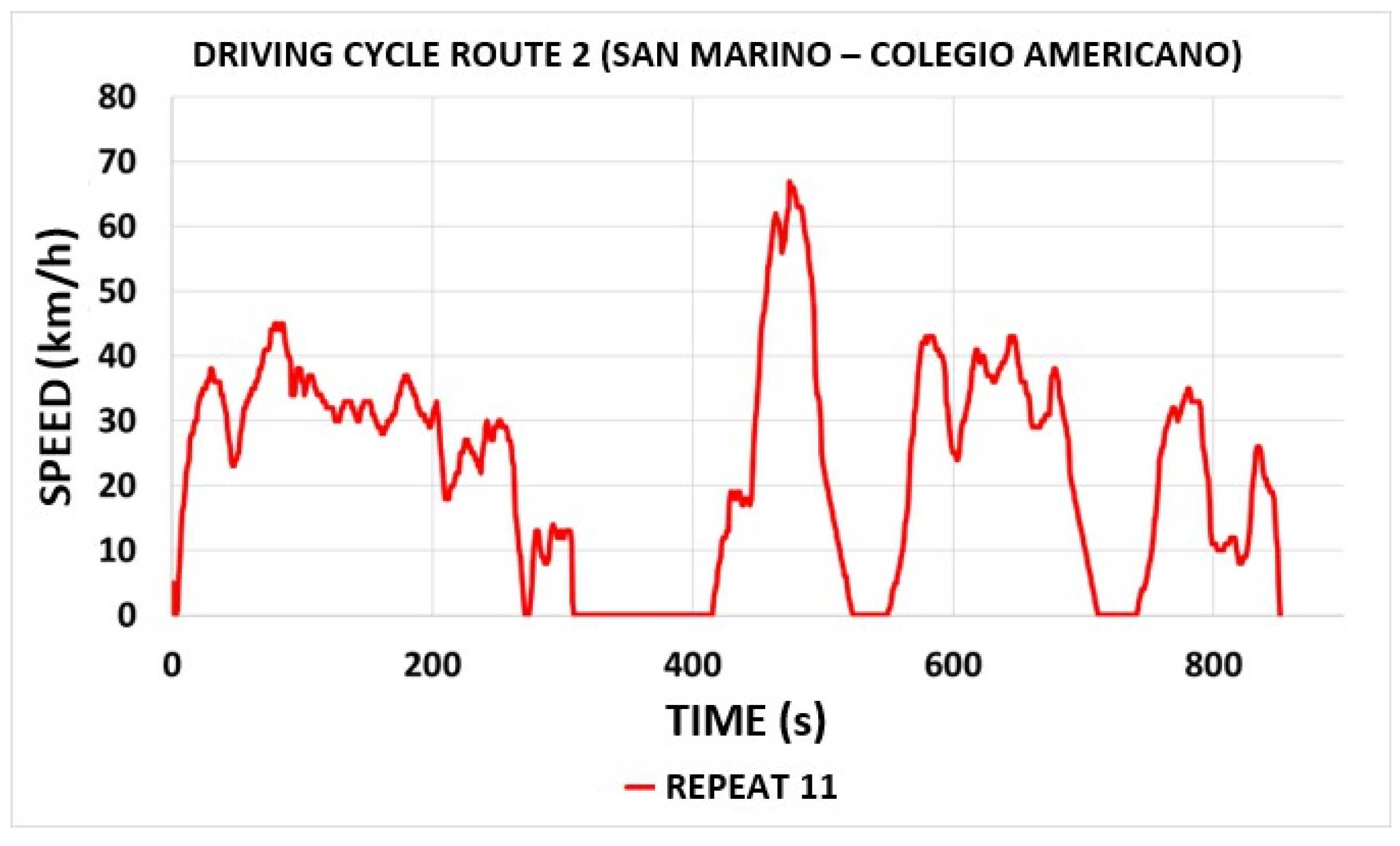
Next, the value of “Y” was calculated for each of the variables in the 11 repetitions and the one with the lowest value was chosen. Thus, it was concluded that the driving cycle associated with Route 2 (San Marino Shopping - Colegio Americano), among the 11 repetitions, corresponds to repetition number 11, as shown in Table 11.
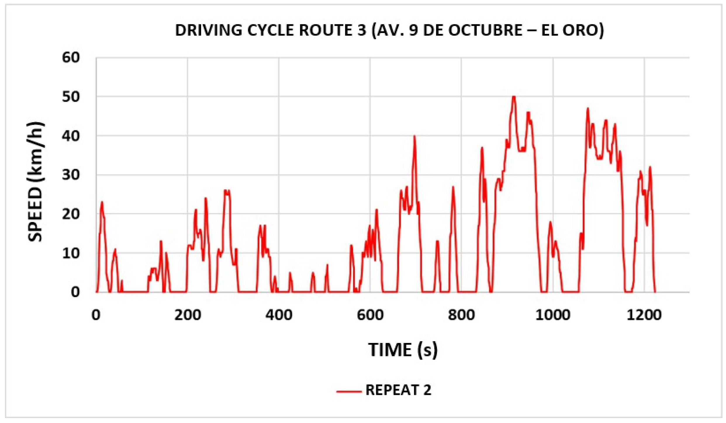
Then, the value of “Y” was calculated for each of the variables in the 11 repetitions and the one with the lowest value was chosen. Thus, it was concluded that the driving cycle associated with Route 3 (Av. 9 de Octubre - El Oro), among the 11 repetitions, corresponds to repetition number 2, as shown in Table 12.
Finally, the value of “Y” was calculated for each of the variables in the 11 repetitions and the one with the lowest value was chosen. Thus, it was concluded that the driving cycle associated with Route 4 (UPS Centenario - 17th Street and Portete), among the 11 repetitions, corresponds to repetition number 5, as shown in Table 13.
3.6. Characteristic Curves
3.6.1. Route 1 (Via a la Costa - Peaje)
3.6.2. Route 2 (San Marino - Colegio Americano)
3.6.3. Route 3 (Av. 9 de Octubre - El Oro)
3.6.4. Route 4 (UPS Centenario - Calle 17 y Portete)
3.7. Comparisons with Other Driving Cycles
The driving cycles in Guayaquil show significant differences compared to standardized cycles (FTP-75, HWFET, and NEDC). Vía a la Costa has the highest average speed (65.39 km/h), similar to HWFET (77.7 km/h), while Route 3 and WSL have the lowest speeds (11.05 km/h and 6.7 km/h, respectively), indicating more congested traffic. In terms of maximum speed, NEDC leads with 120.09 km/h, far exceeding the values recorded in Guayaquil. Route 3 has the highest number of stops (18), similar to FTP-75 (16), reflecting more stop-and-go traffic conditions. Regarding driving time, NEDC is the longest (1633 s), followed by Route 3 (1223 s). Idling time is significantly high in Route 3 (613 s) and in FTP-75 and NEDC cycles (241 s), showing prolonged traffic standstills.
In terms of distance traveled, NEDC has the highest value (17,786 m), while Route 3 records the lowest (3,900 m), confirming its heavy congestion. For the proportion of driving time, HWFET and Vía a la Costa stand out with values close to 100 percent, indicating smooth traffic flow, whereas Route 3 (49.89 percent) and NEDC (79.58 percent) show lower efficiency. Finally, acceleration time is highest in Vía a la Costa (75.58 percent), surpassing the standardized cycles, suggesting more dynamic driving conditions in this area. As shown in Table 18.
The driving conditions in Guayaquil, Cuenca, and Quito vary significantly. Vía a la Costa and Quito / Highway have the highest average speeds (65.39 km/h and 65.98 km/h, respectively), while Guayaquil / Route 3 (11.05 km/h) and Quito / City (13.26 km/h) show the lowest speeds, indicating heavy congestion. In terms of maximum speed, Quito / Highway leads with 89.91 km/h, followed by Vía a la Costa (79 km/h), while Guayaquil / Route 3 (50 km/h) and Quito / City (45.77 km/h) have the lowest values, reflecting urban traffic conditions. Quito / Combined and Quito / City experience the highest number of stops (63 and 58, respectively), suggesting frequent traffic interruptions, whereas Vía a la Costa and Quito / Highway have the fewest stops (0 and 2, respectively), indicating smoother driving.
Guayaquil / Route 3 has the longest idling time (613 s), similar to Quito / Cobined
(960 s) and Quito / City (1060 s), reinforcing their high congestion levels. Regarding distance traveled, Quito / Highway leads (27,463 m), followed by Quito / Combined (15,673 m) and Vía a la Costa (14,901 m), while Guayaquil / Route 3 records the shortest distance (3,900 m). Quito / Highway and Vía a la Costa also have the longest acceleration times (791 s and 556 s, respectively), suggesting dynamic driving conditions. The proportion of driving time and acceleration mode is highest in Vía a la Costa (98.64 percent and 75.58 percent, respectively), indicating efficient traffic flow, while urban areas such as Guayaquil / Route 3 and Quito / City exhibit lower values, reflecting stop-and-go conditions. As shown in Table 19.
The driving conditions across Guayaquil, Esmeraldas, and the Ambato-Riobamba 393 route show notable differences. Vía a la Costa and Ambato-Riobamba / Highway have the highest average speeds (65.39 km/h and 60.95 km/h, respectively), indicating smooth traffic flow, while Guayaquil / Route 3 (11.05 km/h) has the lowest, reflecting heavy congestion. In terms of maximum speed, Ambato-Riobamba / Highway leads with 120.4 km/h, far exceeding values recorded in Guayaquil. The number of stops is highest in Guayaquil / Route 3 (18), similar to Ambato-Riobamba / Urban (13), suggesting frequent interruptions, while Vía a la Costa and Ambato-Riobamba / Highway (0 and 2 stops, respectively) experience the most continuous traffic. Guayaquil / Route 3 also has the longest idling time (613 s), reinforcing its congested conditions.
Regarding driving time, Esmeraldas records 1,750 s, longer than any Guayaquil area but shorter than Ambato-Riobamba / Highway (2,500 s), which is expected for a highway route. The longest distance traveled is in Esmeraldas (15,420 m), surpassing Vía a la Costa (14,901 m), while Guayaquil / Route 3 has the shortest (3,900 m). The proportion of driving time is highest in Ambato-Riobamba / Highway (96.06 percent), similar to Vía a la Costa (98.64 percent), confirming smoother traffic conditions, while Guayaquil / Route 3 (49.89 percent) has the lowest value, indicating frequent stops and idling. Overall, highway routes such as Ambato-Riobamba / Highway and Vía a la Costa show the best driving efficiency, whereas urban areas like Guayaquil / Route 3 experience heavy congestion and frequent traffic interruptions. As shown in Table 20.
4. Discussion
The analysis of the driving conditions on the different routes evaluated reveals significant differences in terms of efficiency and fluidity, as shown in Table A1 of Appendix A. Route 1, which corresponds to the Via a la Costa - Peaje (VC) is the fastest route, with an average speed of 65.39 km/h and a maximum speed of 79 km/h, without stops and with only 10 seconds in idling. In contrast, Route 3 comprising the Downtown sector (C) is the most congested, with an average speed of just 11.05 km/h and a high idling time of 613 seconds, reflecting dense traffic and numerous interruptions.
The intermediate routes, Route 2 starting at the San Marino Shopping Center to the American School (SM) and Route 4, comprising UPS Centenario and, 17th Street and Portete (P), present mixed characteristics. San Marino has an average speed of 21.39 km/h and a maximum speed of 67 km/h, with an idling time of 243 seconds, while Portete shows an average speed of 16.27 km/h and a maximum speed of 39 km/h, with 247 seconds at idle. Both routes maintain relatively high active driving (71.41 percent and 74.30 percent, respectively), although with greater fluctuations in speed due to multiple stops and frequent accelerations.
In terms of stability and efficiency, the Via a la Costa (VC) stands out as the best option, with a continuous and uninterrupted route. On the other hand, the Downtown sector (C) is the least efficient route due to high congestion and long stopping times. San Marino (SM) and Portete (P) fall somewhere in between, with variable traffic conditions, but less critical than Downtown (C). These results underscore the importance of effective road planning to improve mobility in the most congested areas.
According to Table 18, when comparing Guayaquil’s driving cycles with foreign cycles, key differences in speed, stops and vehicle flow are observed. The Via a la Costa (VC), similar to the HWFET (Highway Fuel Economy Test), has high speeds (65.39 km/h vs. 77.7 km/h), no stops and a driving time of over 98 percent. On the other hand, the Downtown (C) cycle, with a top speed of 50 km/h and a driving time of 1,223.4 seconds, shows a performance close to the WSL, although with a higher acceleration ratio (27.14 percent) compared to the WSL (30.52 percent). Finally, the NEDC (with a top speed of 120.09 km/h and 23.56 percent acceleration) has a different behavior, with higher top speed and less acceleration. However, the Downtown (C), San Marino (SM) and Portete (P) routes show similar trends to those of the ECE-15, an urban section of the NEDC. In summary, the Guayaquil cycles, especially the one on Via a la Costa, are more dynamic, while the Downtown (C) cycle is more similar to the WSL due to its low speed and long driving time [18,43].
On the other hand, according to Table 19, the comparison of driving cycles in Guayaquil, Quito and Cuenca shows that Via a la Costa (VC) and Quito/Carretera have the best flow conditions, with high speeds ( 65 km/h), few stops and minimal idling time. In contrast, Guayaquil Route 3 (C) and Quito/Ciudad have dense traffic, with low speeds (11-13 km/h) and multiple stops. San Marino (SM), Portete (P) and Cuenca reflect intermediate conditions, with moderate speeds and frequent interruptions. In addition, Via a la Costa (VC) had the longest time in acceleration (75.58 percent), while Route 3 (C) and Cuenca showed lower fluidity (27-36 percent), highlighting key differences in urban mobility [18].
Finally, according to Table 20, the comparison of driving cycles in Guayaquil, Esmeraldas and Ambato-Riobamba shows that Via a la Costa and the Ambato-Riobamba highway have the best flow conditions, with high speeds ( 60-65 km/h), few stops and a high proportion of driving time (>96 percent). In contrast, downtown Guayaquil has the densest traffic, with low speeds (11.05 km/h), multiple stops (18) and long idling times. San Marino, Portete and the Ambato-Riobamba urban area reflect intermediate conditions, with moderate speeds (16-26 km/h) and frequent interruptions. These results show differences in mobility and traffic efficiency between cities and road types [16,17].
5. Conclusions
In this study, driving cycles were determined for the four selected routes in the city of Guayaquil. It was concluded that it was not possible to develop a general driving cycle that would represent the entire city due to its large geographic extension, which made it difficult to cover all the zones. However, it was possible to characterize the cycle of each of the selected zones, obtaining a total of four cycles. For this purpose, the direct method was used, based on the collection of real traffic data. The ON BOARD technique was implemented, in which an M1 category vehicle was instrumented, and three drivers were assigned to simulate real traffic conditions, following an approach similar to the American FTP-75 cycle. Speed, time and distance data were collected using the OBDLINK MX+ device and processed in the OBDWiz software, whose outputs were imported into Microsoft Excel. Through a descriptive analysis performed in Minitab, the sample size was determined, which consisted of a total of 45 repetitions distributed among all routes.Likewise, in the data processing, weighting criteria were applied, which made it possible to select the representative cycle for each of the routes analyzed.
The traffic analysis carried out in this study made it possible to identify the characteristics and differences in the vehicular behavior of the main routes selected in Guayaquil. The results show a marked variability in traffic conditions, with highly congested areas, such as in the downtown sector, and others with fluid traffic, such as the route comprising Via a la Costa. Each of the routes was characterized with the help of a GPS application such as Google Maps, which indicated the routes with the most traffic, since it shows the traffic conditions in real time, indicating areas with congestion, accidents and other obstacles.
The analysis showed notable differences between the routes in Guayaquil. Via a la Costa (VC) stood out for its high efficiency, with an average speed of 65.39 km/h, no stops and only 10 seconds idling, reflecting smooth and constant traffic. In contrast, San Marino (SM) presented an average speed of 21.39 km/h, with 4 stops and 243 seconds idling, showing intermediate conditions. Route 3 (C), with an average speed of 11.05 km/h, had the worst conditions, with 18 stops and 613 seconds idling, showing high congestion. Finally, the Portete (P) route, with an average speed of 16.27 km/h, showed similar conditions to San Marino, with 11 stops and 247 seconds idling, indicating moderate traffic flow but with some interruptions. In summary, Via a la Costa showed the best driving conditions, while Downtown experienced more congestion.
Compared to other driving cycles in Ecuador, Guayaquil presents a mix of characteristics. Via a la Costa shows similarities to Quito’s interurban roads, noted for smoother traffic and higher speeds. In contrast, the Route 3 and San Marino routes are more similar to those of Quito/City and Cuenca, where dense traffic and reduced speeds predominate.These results underscore the need to improve road infrastructure in the most congested areas to reduce travel times, emissions and fuel consumption.
Abbreviations
The following abbreviations are used in this manuscript:
| CO | Carbon monoxide |
| CO2 | Carbon dioxide |
| NOx | Nitrogen oxides |
| UHC | Unburned hydrocarbons |
| DC | Driving Cycle |
| UPS | Universidad Politecnica Salesiana del Ecuador |
| N | Number of stops |
| N.P. | Normality test |
| VC | Via a la Costa-Peaje, Route 1 |
| SM | San Marino-Colegio Americano, Route 2 |
| C | Av. 9 de Octubre-El Oro, Route 3 |
| P | UPS Centenario-Calle 17 y Portete, Route 4 |
| m | Meters |
| s | Second |
| R | Repetitions |
Appendix A
Table A1.
Final results corresponding to each Route.
| Routes | Average speed (km/h) | Max. speed (km/h) |
N | Driving time (s) | Idle time (s) | Distance (m) | Positive acceleration time (s) | % of driving time | % of time accelerating |
|---|---|---|---|---|---|---|---|---|---|
| VC | 65,39 | 79 | 0 | 735,624 | 10 | 14901 | 556 | 98,64 | 75,58 |
| SM | 21,39 | 67 | 4 | 850,091 | 243 | 5712 | 306 | 71,41 | 36,00 |
| C | 11,05 | 50 | 18 | 1223,416 | 613 | 3900 | 332 | 49,89 | 27,14 |
| P | 16,27 | 39 | 11 | 961,223 | 247 | 4689 | 374 | 74,30 | 38,91 |
Table A2.
Calculation of the deviation from the median of Route 1.
| R | Average speed (km/h) | Max. speed (km/h) |
N | Driving time (s) | Idle time (s) | Distance (m) | Positive acceleration time (s) | % of driving time | % of time accelerating |
|---|---|---|---|---|---|---|---|---|---|
| 1 | 0.016274 | 0 | 0 | 0.010037 | 0.523810 | 0.000571 | 0.065868 | 0.007476 | 0.062303 |
| 2 | 0.028556 | 0.126582 | 0 | 0.039066 | 0.142857 | 0.000034 | 0.033362 | 0.001450 | 0.012633 |
| 3 | 0.005402 | 0.050633 | 0 | 0.016939 | 0.047619 | 0.000235 | 0.012831 | 0.001039 | 0.037143 |
| 4 | 0.000820 | 0.025316 | 0 | 0.025643 | 0.238095 | 0.000839 | 0.005988 | 0.003067 | 0.012633 |
| 5 | 0.032539 | 0.101266 | 0 | 0.039390 | 0.142857 | 0.000034 | 0.144568 | 0.002817 | 0.103562 |
| 6 | 0.008739 | 0.117647 | 0 | 0.016889 | 0.809524 | 0.000369 | 0.053892 | 0.012145 | 0.031231 |
| 7 | 0.000820 | 0 | 0 | 0.010037 | 0.047619 | 0.000168 | 0.048760 | 0.000446 | 0.032718 |
| 8 | 0.085888 | 0.025316 | 0 | 0.117994 | 0.238095 | 0.000101 | 0.141146 | 0.004466 | 0.027505 |
| 9 | 0.054633 | 0.075949 | 0 | 0.051277 | 0.333333 | 0.000571 | 0.005988 | 0.005145 | 0.048176 |
| 10 | 0.022249 | 0 | 0 | 0.010167 | 0.428571 | 0.000705 | 0.031651 | 0.006126 | 0.035015 |
| 11 | 0.013073 | 0.063291 | 0 | 0.024334 | 0.238095 | 0.000369 | 0.117194 | 0.003953 | 0.152682 |
| 12 | 0.085169 | 0.063291 | 0 | 0.115808 | 0.142857 | 0.000168 | 0.137725 | 0.000446 | 0.026431 |
Table A3.
Determination of the “Y” value for each repetition of Route 1.
| R | Average speed (km/h) | Max. speed (km/h) | N | Driving time (s) | Idle time (s) | Distance (m) | Positive acceleration time (s) | % of driving time | % of time accelerating | Weighted Median (Y) |
|---|---|---|---|---|---|---|---|---|---|---|
| 1 | 0,002504 | 0,000000 | 0 | 0,001544 | 0,060440 | 0,000088 | 0,002533 | 0,001150 | 0,009585 | 0,077843793 |
| 2 | 0,004393 | 0,004869 | 0 | 0,006010 | 0,016484 | 0,000005 | 0,001283 | 0,000223 | 0,001944 | 0,035210292 |
| 3 | 0,000831 | 0,001947 | 0 | 0,002606 | 0,005495 | 0,000036 | 0,000494 | 0,000160 | 0,005714 | 0,017282947 |
| 4 | 0,000126 | 0,000974 | 0 | 0,003945 | 0,027473 | 0,000129 | 0,000230 | 0,000472 | 0,001944 | 0,035292337 |
| 5 | 0,005006 | 0,003895 | 0 | 0,006060 | 0,016484 | 0,000005 | 0,005560 | 0,000433 | 0,015933 | 0,053375852 |
| 6 | 0,001344 | 0,004525 | 0 | 0,002598 | 0,093407 | 0,000057 | 0,002073 | 0,001869 | 0,004805 | 0,110677161 |
| 7 | 0,000126 | 0,000000 | 0 | 0,001544 | 0,005495 | 0,000026 | 0,001875 | 0,000069 | 0,005034 | 0,014168079 |
| 8 | 0,013214 | 0,000974 | 0 | 0,018153 | 0,027473 | 0,000015 | 0,005429 | 0,000687 | 0,004232 | 0,07017558 |
| 9 | 0,008405 | 0,002921 | 0 | 0,007889 | 0,038462 | 0,000088 | 0,000230 | 0,000792 | 0,007412 | 0,06619794 |
| 10 | 0,003423 | 0,000000 | 0 | 0,001564 | 0,049451 | 0,000108 | 0,001217 | 0,000942 | 0,005387 | 0,062092846 |
| 11 | 0,002011 | 0,002434 | 0 | 0,003744 | 0,027473 | 0,000057 | 0,004507 | 0,000608 | 0,023489 | 0,064323663 |
| 12 | 0,013103 | 0,002434 | 0 | 0,017817 | 0,016484 | 0,000026 | 0,005297 | 0,000069 | 0,004066 | 0,059295068 |
Table A4.
Calculation of the deviation from the median of Route 2.
| R | Average speed (km/h) | Max. speed (km/h) |
N | Driving time (s) | Idle time (s) | Distance (m) | Positive acceleration time (s) | % of driving time | % of time accelerating |
|---|---|---|---|---|---|---|---|---|---|
| 1 | 0,137035 | 0 | 0,166667 | 0,110643 | 0,236641 | 0,001404 | 0,094771 | 0,056358 | 0,051534 |
| 2 | 0,131701 | 0,093750 | 0,000000 | 0,116548 | 0,431298 | 0,001404 | 0,032680 | 0,151356 | 0,207600 |
| 3 | 0,018823 | 0,031250 | 0,166667 | 0,005257 | 0,072519 | 0,000000 | 0,035948 | 0,040969 | 0,075890 |
| 4 | 0,031945 | 0,156250 | 0,166667 | 0,038275 | 0,000000 | 0,000175 | 0,068627 | 0,009961 | 0,073273 |
| 5 | 0,140971 | 0,031250 | 0,166667 | 0,173381 | 0,622137 | 0,001930 | 0,022876 | 0,175658 | 0,099415 |
| 6 | 0,004619 | 0,294118 | 0,166667 | 0,006802 | 0,164122 | 0,000175 | 0,029412 | 0,075529 | 0,004063 |
| 7 | 0,201378 | 0,031250 | 0,333333 | 0,159871 | 0,190840 | 0,002106 | 0,192810 | 0,009960 | 0,007409 |
| 8 | 0,045998 | 0,031250 | 0,333333 | 0,056729 | 0,263359 | 0,000351 | 0,022876 | 0,092917 | 0,000000 |
| 9 | 0,106995 | 0,046875 | 0,333333 | 0,110921 | 0,446565 | 0,001579 | 0,016340 | 0,140104 | 0,085249 |
| 10 | 0,030177 | 0,031250 | 0,333333 | 0,035770 | 0,049618 | 0,000702 | 0,042484 | 0,000000 | 0,116939 |
| 11 | 0,000000 | 0,046875 | 0,333333 | 0,000000 | 0,072519 | 0,002281 | 0,000000 | 0,025745 | 0,033096 |
Table A5.
Determination of the “Y” value for each repetition of Route 2.
| R | Average speed (km/h) | Max. speed (km/h) | N | Driving time (s) | Idle time (s) | Distance (m) | Positive acceleration time (s) | % of driving time | % of time accelerating | Weighted Median (Y) |
|---|---|---|---|---|---|---|---|---|---|---|
| 1 | 0,021082 | 0,000000 | 0,006410 | 0,017022 | 0,027305 | 0,000216 | 0,003645 | 0,008670 | 0,007928 | 0,092290 |
| 2 | 0,020262 | 0,003606 | 0,000000 | 0,017930 | 0,049765 | 0,000216 | 0,001257 | 0,023286 | 0,031939 | 0,1482599 |
| 3 | 0,002896 | 0,001202 | 0,006410 | 0,000809 | 0,008368 | 0,000000 | 0,001383 | 0,006303 | 0,011675 | 0,0390453 |
| 4 | 0,004915 | 0,006010 | 0,006410 | 0,005888 | 0,000000 | 0,000027 | 0,002640 | 0,001532 | 0,011273 | 0,0386946 |
| 5 | 0,021688 | 0,001202 | 0,006410 | 0,026674 | 0,071785 | 0,000297 | 0,000880 | 0,027024 | 0,015295 | 0,1712550 |
| 6 | 0,000711 | 0,011312 | 0,006410 | 0,001046 | 0,018937 | 0,000027 | 0,001131 | 0,011620 | 0,000625 | 0,0518198 |
| 7 | 0,030981 | 0,001202 | 0,012821 | 0,024596 | 0,022020 | 0,000324 | 0,007416 | 0,001532 | 0,001140 | 0,1020311 |
| 8 | 0,007077 | 0,001202 | 0,012821 | 0,008728 | 0,030388 | 0,000054 | 0,000880 | 0,014295 | 0,000000 | 0,0754430 |
| 9 | 0,016461 | 0,001803 | 0,012821 | 0,017065 | 0,051527 | 0,000243 | 0,000628 | 0,021554 | 0,013115 | 0,1352169 |
| 10 | 0,004643 | 0,001202 | 0,012821 | 0,005503 | 0,005725 | 0,000108 | 0,001634 | 0,000000 | 0,017991 | 0,0496261 |
| 11 | 0,000000 | 0,001803 | 0,012821 | 0,000000 | 0,008368 | 0,000351 | 0,000000 | 0,003961 | 0,005092 | 0,0323944 |
Table A6.
Calculation of the deviation from the median of Route 3.
| R | Average speed (km/h) | Max. speed (km/h) | N | Driving time (s) | Idle time (s) | Distance (m) | Positive acceleration time (s) | % of driving time | % of time accelerating |
|---|---|---|---|---|---|---|---|---|---|
| 1 | 0.13115 | 0.18000 | 0.26316 | 0.11305 | 0.31974 | 0.00000 | 0.00000 | 0.25155 | 0.11385 |
| 2 | 0.03882 | 0.00000 | 0.05263 | 0.02946 | 0.00000 | 0.00026 | 0.00606 | 0.00410 | 0.02408 |
| 3 | 0.07322 | 0.06000 | 0.26316 | 0.07063 | 0.10277 | 0.00026 | 0.11212 | 0.00378 | 0.02621 |
| 4 | 0.10818 | 0.06000 | 0.05263 | 0.11666 | 0.23654 | 0.00487 | 0.13030 | 0.07885 | 0.00000 |
| 5 | 0.09996 | 0.02000 | 0.15789 | 0.10387 | 0.14356 | 0.00051 | 0.10000 | 0.00953 | 0.01554 |
| 6 | 0.02810 | 0.23529 | 0.10526 | 0.02469 | 0.04078 | 0.00128 | 0.03333 | 0.03980 | 0.02082 |
| 7 | 0.00000 | 0.14000 | 0.15789 | 0.00000 | 0.00979 | 0.00077 | 0.16364 | 0.03486 | 0.14959 |
| 8 | 0.01232 | 0.12000 | 0.00000 | 0.00419 | 0.08972 | 0.00282 | 0.03030 | 0.11614 | 0.04601 |
| 9 | 0.11493 | 0.04000 | 0.05263 | 0.09536 | 0.12398 | 0.00180 | 0.00909 | 0.00000 | 0.10628 |
| 10 | 0.63906 | 0.16000 | 0.47368 | 0.39497 | 0.61990 | 0.00103 | 0.12121 | 0.38622 | 0.43493 |
| 11 | 0.05698 | 0.06000 | 0.15789 | 0.05829 | 0.12887 | 0.00051 | 0.05758 | 0.09812 | 0.01132 |
Table A7.
Determination of the “Y” value for each repetition of Route 3.
| R | Average speed (km/h) | Max. speed (km/h) | N | Driving time (s) | Idle time (s) | Distance (m) | Positive acceleration time (s) | % of driving time | % of time accelerating | Weighted Median (Y) |
|---|---|---|---|---|---|---|---|---|---|---|
| 1 | 0,020177 | 0,006923 | 0,010121 | 0,017393 | 0,036893 | 0,000000 | 0,000000 | 0,038701 | 0,017515 | 0,14772333 |
| 2 | 0,005972 | 0,000000 | 0,002024 | 0,004532 | 0,000000 | 0,000039 | 0,000233 | 0,000631 | 0,003705 | 0,01713682 |
| 3 | 0,011265 | 0,002308 | 0,010121 | 0,010866 | 0,011858 | 0,000039 | 0,004312 | 0,000582 | 0,004033 | 0,05538475 |
| 4 | 0,016643 | 0,002308 | 0,002024 | 0,017947 | 0,027293 | 0,000750 | 0,005012 | 0,012130 | 0,000000 | 0,08410724 |
| 5 | 0,015379 | 0,000769 | 0,006073 | 0,015980 | 0,016564 | 0,000079 | 0,003846 | 0,001467 | 0,002391 | 0,06254757 |
| 6 | 0,004322 | 0,009050 | 0,004049 | 0,003799 | 0,004706 | 0,000197 | 0,001282 | 0,006124 | 0,003204 | 0,03673217 |
| 7 | 0,000000 | 0,005385 | 0,006073 | 0,000000 | 0,001129 | 0,000118 | 0,006294 | 0,005363 | 0,023014 | 0,04737596 |
| 8 | 0,001895 | 0,004615 | 0,000000 | 0,000645 | 0,010353 | 0,000434 | 0,001166 | 0,017868 | 0,007078 | 0,04405365 |
| 9 | 0,017681 | 0,001538 | 0,002024 | 0,014671 | 0,014305 | 0,000276 | 0,000350 | 0,000000 | 0,016351 | 0,06719662 |
| 10 | 0,098316 | 0,006154 | 0,018219 | 0,060765 | 0,071527 | 0,000158 | 0,004662 | 0,059419 | 0,066913 | 0,38613193 |
| 11 | 0,008766 | 0,002308 | 0,006073 | 0,008968 | 0,014870 | 0,000079 | 0,002214 | 0,015095 | 0,001742 | 0,06011434 |
Table A8.
Calculation of the deviation from the median of Route 4.
| R | Average speed (km/h) | Max. speed (km/h) | N | Driving time (s) | Idle time (s) | Distance (m) | Positive acceleration time (s) | % of driving time | % of time accelerating |
|---|---|---|---|---|---|---|---|---|---|
| 1 | 0.045779 | 0.022727 | 0.181818 | 0.033966 | 0.385542 | 0.000426 | 0.039773 | 0.107084 | 0.000000 |
| 2 | 0.008054 | 0.181818 | 0.363636 | 0.012900 | 0.228916 | 0.000213 | 0.607955 | 0.092665 | 0.754061 |
| 3 | 0.072096 | 0.000000 | 0.090909 | 0.086540 | 0.128514 | 0.000213 | 0.008523 | 0.030872 | 0.188854 |
| 4 | 0.030379 | 0.068182 | 0.181818 | 0.022400 | 0.184739 | 0.001490 | 0.000000 | 0.042304 | 0.053201 |
| 5 | 0.014804 | 0.113636 | 0.000000 | 0.005748 | 0.008032 | 0.002128 | 0.062500 | 0.019345 | 0.137553 |
| 6 | 0.000000 | 0.823529 | 0.090909 | 0.000000 | 0.257028 | 0.002554 | 0.184659 | 0.077418 | 0.122047 |
| 7 | 0.141928 | 0.068182 | 0.454545 | 0.150073 | 0.614458 | 0.001064 | 0.053977 | 0.129873 | 0.013180 |
| 8 | 0.059744 | 0.022727 | 0.272727 | 0.072286 | 0.080321 | 0.001702 | 0.247159 | 0.017544 | 0.126181 |
| 9 | 0.175753 | 0.136364 | 0.363636 | 0.159946 | 0.212851 | 0.000000 | 0.281250 | 0.036958 | 0.078696 |
| 10 | 0.031392 | 0.045455 | 0.090909 | 0.038853 | 0.000000 | 0.000213 | 0.193182 | 0.000000 | 0.096105 |
| 11 | 0.089309 | 0.045455 | 0.181818 | 0.088613 | 0.329317 | 0.000851 | 0.034091 | 0.064581 | 0.022863 |
Table A9.
Determination of the “Y” value for each repetition of Route 4.
| R | Average speed (km/h) | Max. speed (km/h) | N | Driving time (s) | Idle time (s) | Distance (m) | Positive acceleration time (s) | % of driving time | % of time accelerating | Weighted Median (Y) |
|---|---|---|---|---|---|---|---|---|---|---|
| 1 | 0,007043 | 0,000874 | 0,006993 | 0,005225 | 0,044486 | 0,000065 | 0,001530 | 0,016474 | 0,000000 | 0,08269084 |
| 2 | 0,001239 | 0,006993 | 0,013986 | 0,001985 | 0,026413 | 0,000033 | 0,023383 | 0,014256 | 0,116009 | 0,20429729 |
| 3 | 0,011092 | 0,000000 | 0,003497 | 0,013314 | 0,014829 | 0,000033 | 0,000328 | 0,004749 | 0,029054 | 0,07689503 |
| 4 | 0,004674 | 0,002622 | 0,006993 | 0,003446 | 0,021316 | 0,000229 | 0,000000 | 0,006508 | 0,008185 | 0,05397343 |
| 5 | 0,002278 | 0,004371 | 0,000000 | 0,000884 | 0,000927 | 0,000327 | 0,002404 | 0,002976 | 0,021162 | 0,03532883 |
| 6 | 0,000000 | 0,031674 | 0,003497 | 0,000000 | 0,029657 | 0,000393 | 0,007102 | 0,011911 | 0,018776 | 0,10300991 |
| 7 | 0,021835 | 0,002622 | 0,017483 | 0,023088 | 0,070899 | 0,000164 | 0,002076 | 0,019980 | 0,002028 | 0,16017498 |
| 8 | 0,009191 | 0,000874 | 0,010490 | 0,011121 | 0,009268 | 0,000262 | 0,009506 | 0,002699 | 0,019413 | 0,07282350 |
| 9 | 0,027039 | 0,005245 | 0,013986 | 0,024607 | 0,024560 | 0,000000 | 0,010817 | 0,005686 | 0,012107 | 0,12404682 |
| 10 | 0,004830 | 0,001748 | 0,003497 | 0,005977 | 0,000000 | 0,000033 | 0,007430 | 0,000000 | 0,014785 | 0,03829988 |
| 11 | 0,013740 | 0,001748 | 0,006993 | 0,013633 | 0,037998 | 0,000131 | 0,001311 | 0,009936 | 0,003517 | 0,08900704 |
Appendix B
Figure A1.
Data obtained from the 12 repetitions of Route 1.
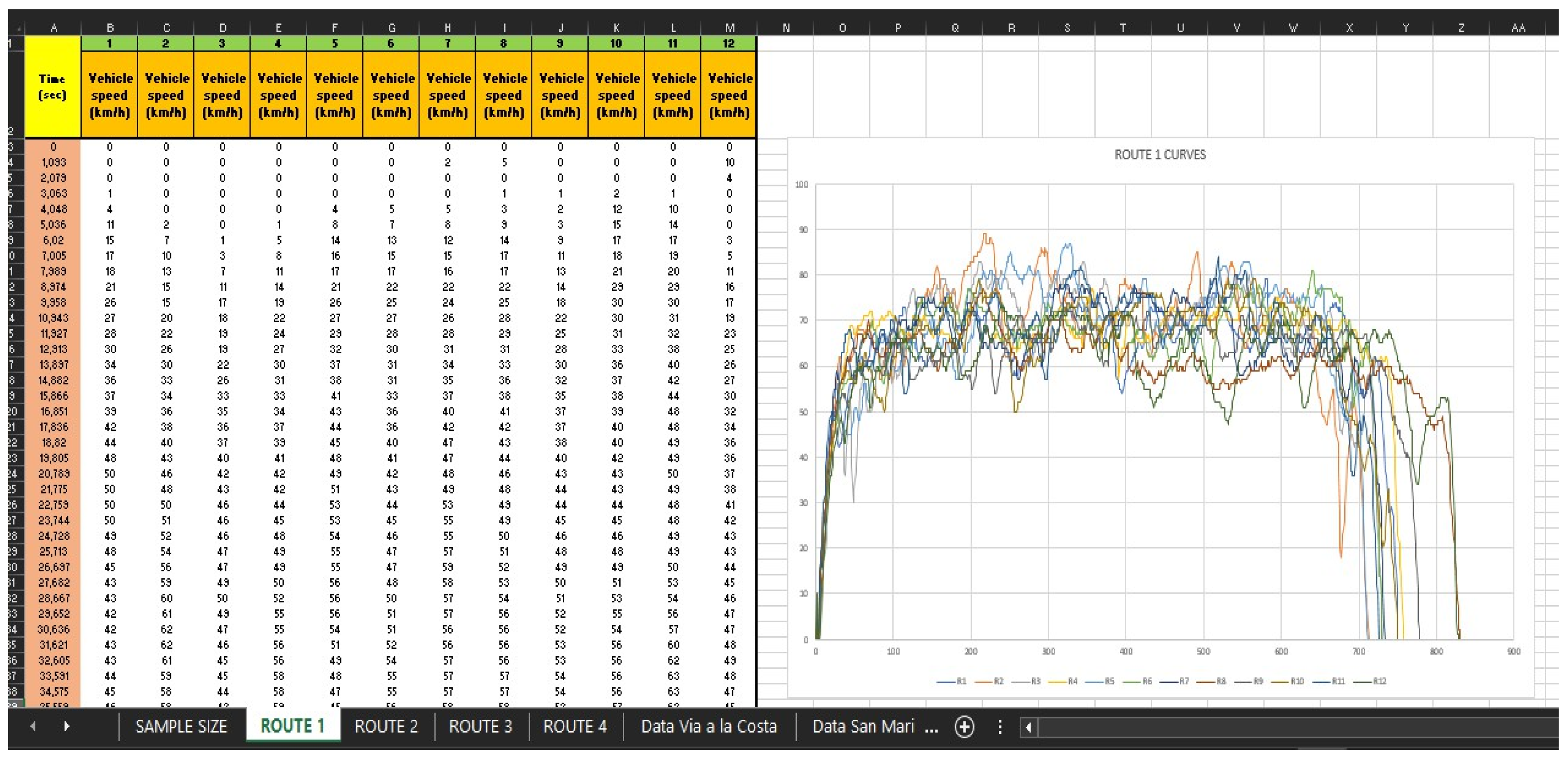
Figure A2.
Scatter plot of Route 1.
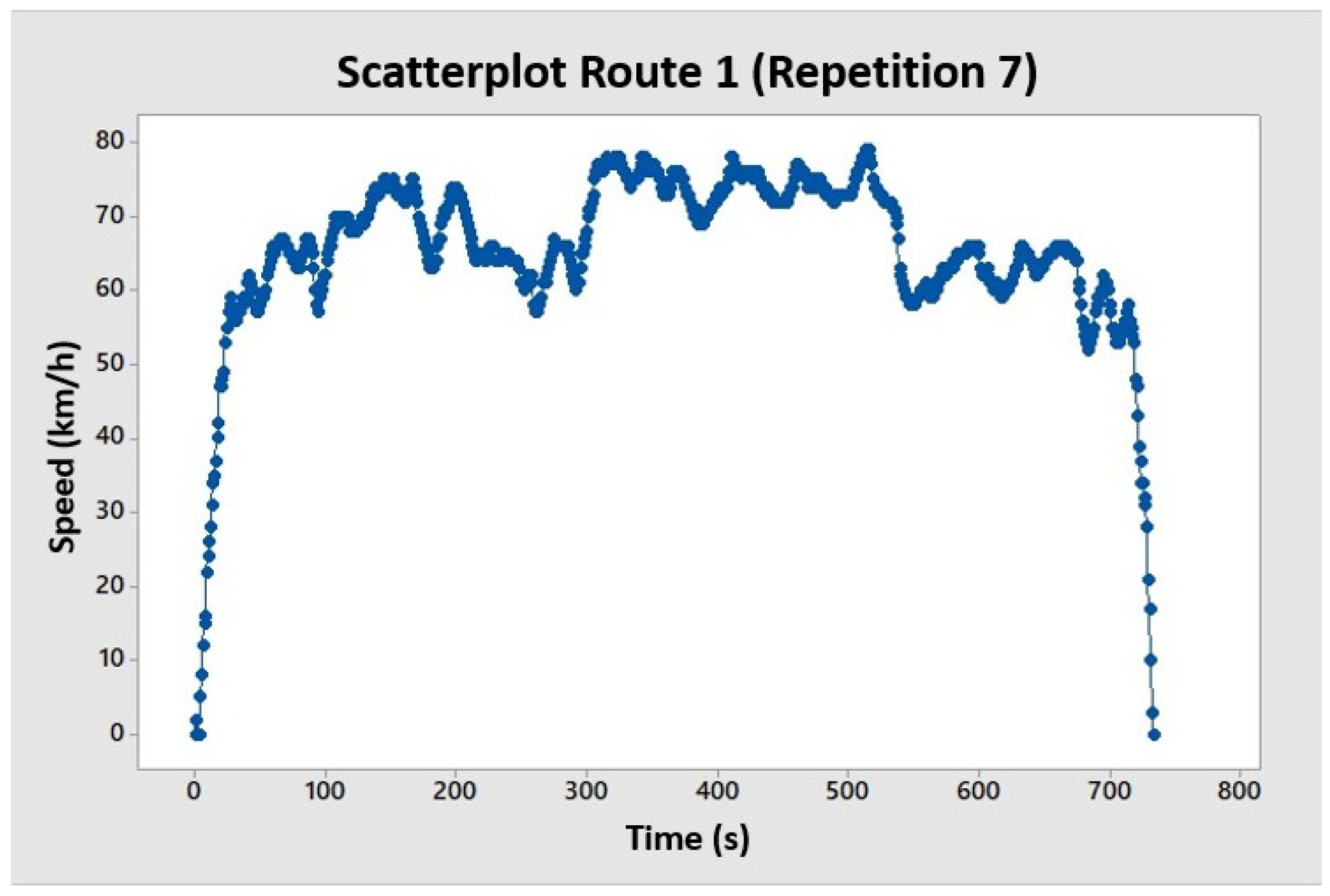
Figure A3.
Data obtained from the 11 repetitions of Route 2.
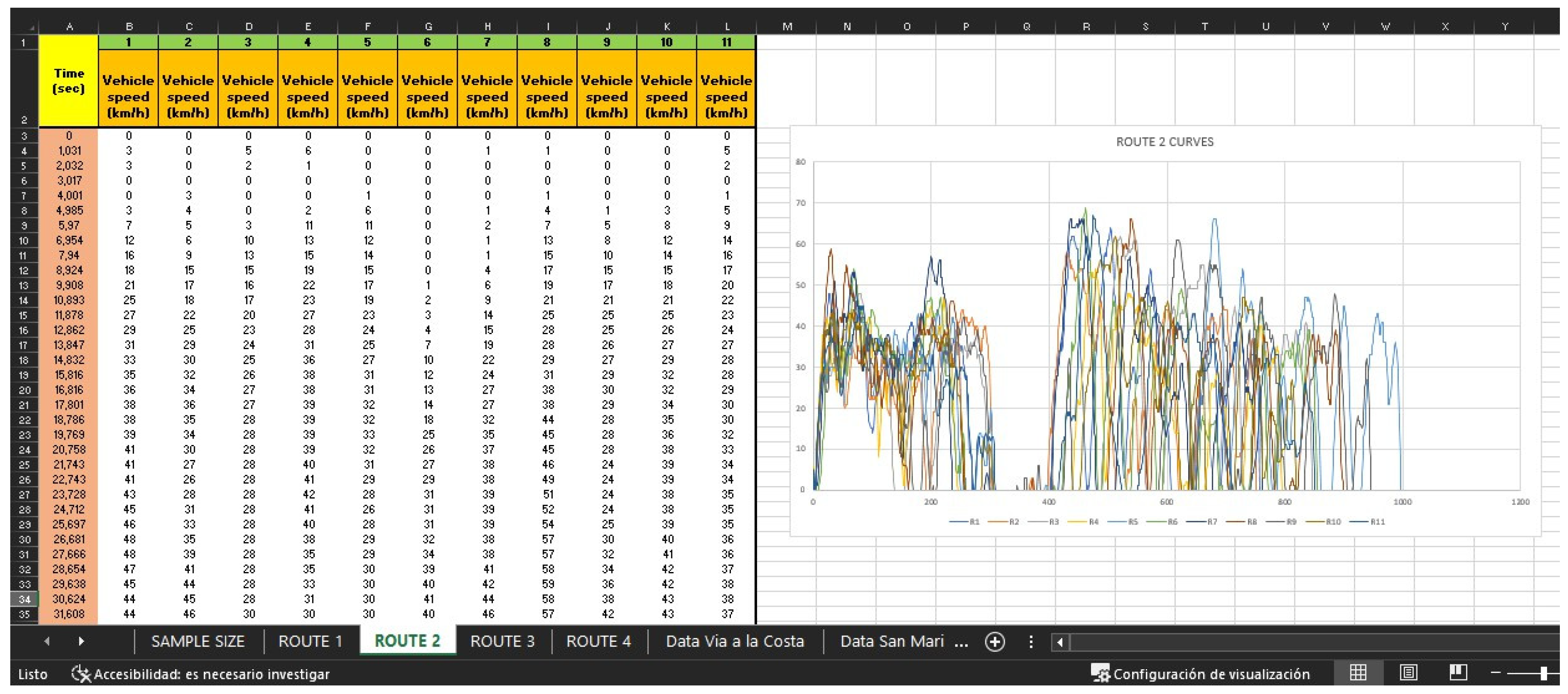
Figure A4.
Scatter plot of Route 2.
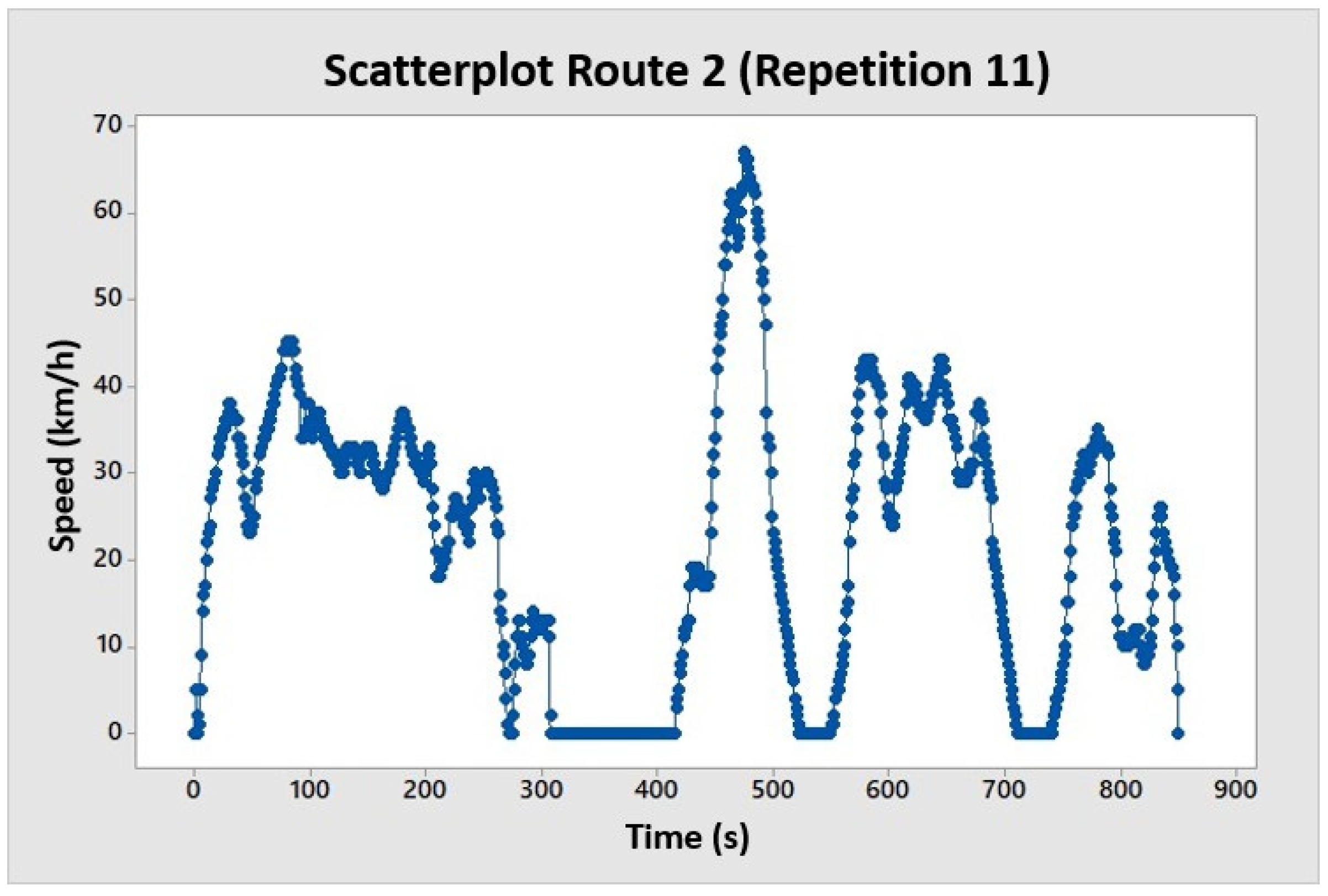
Figure A5.
Data obtained from the 11 repetitions of Route 3.
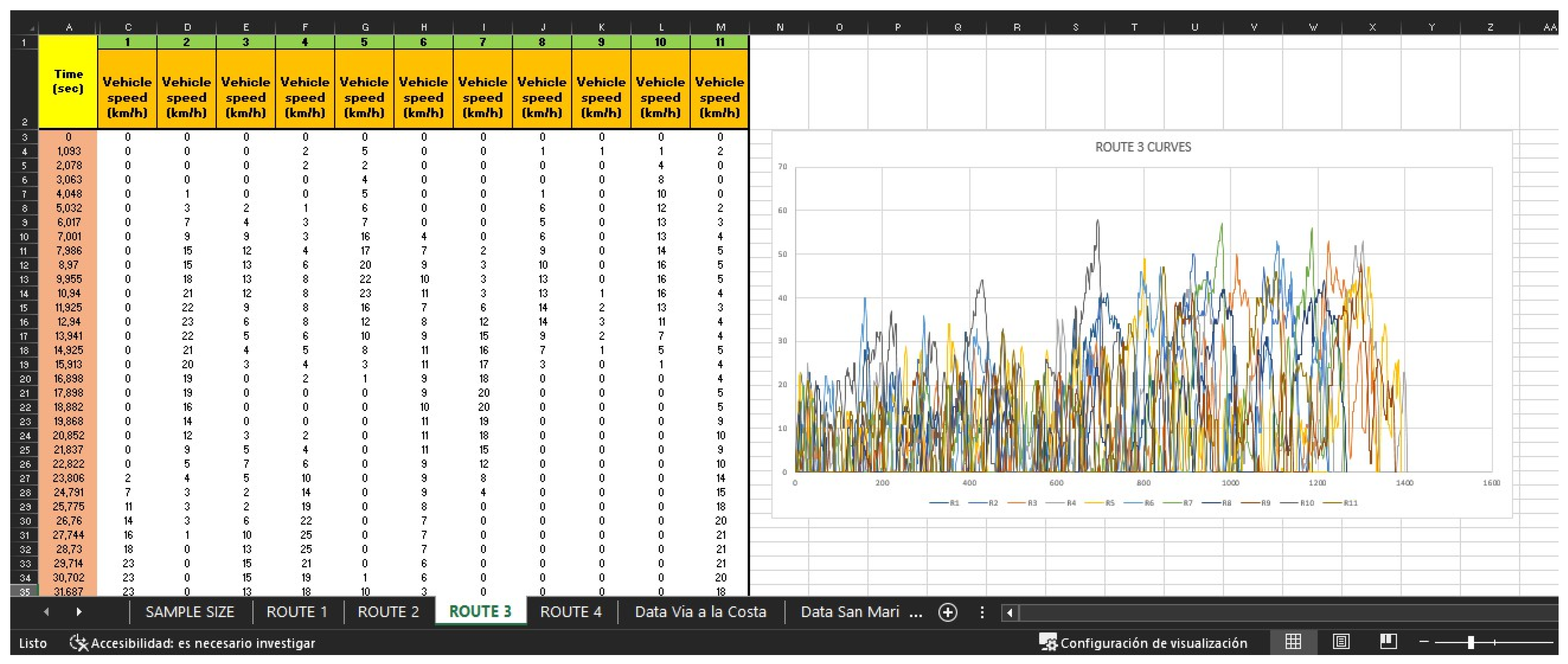
Figure A6.
Scatter plot of Route 3.
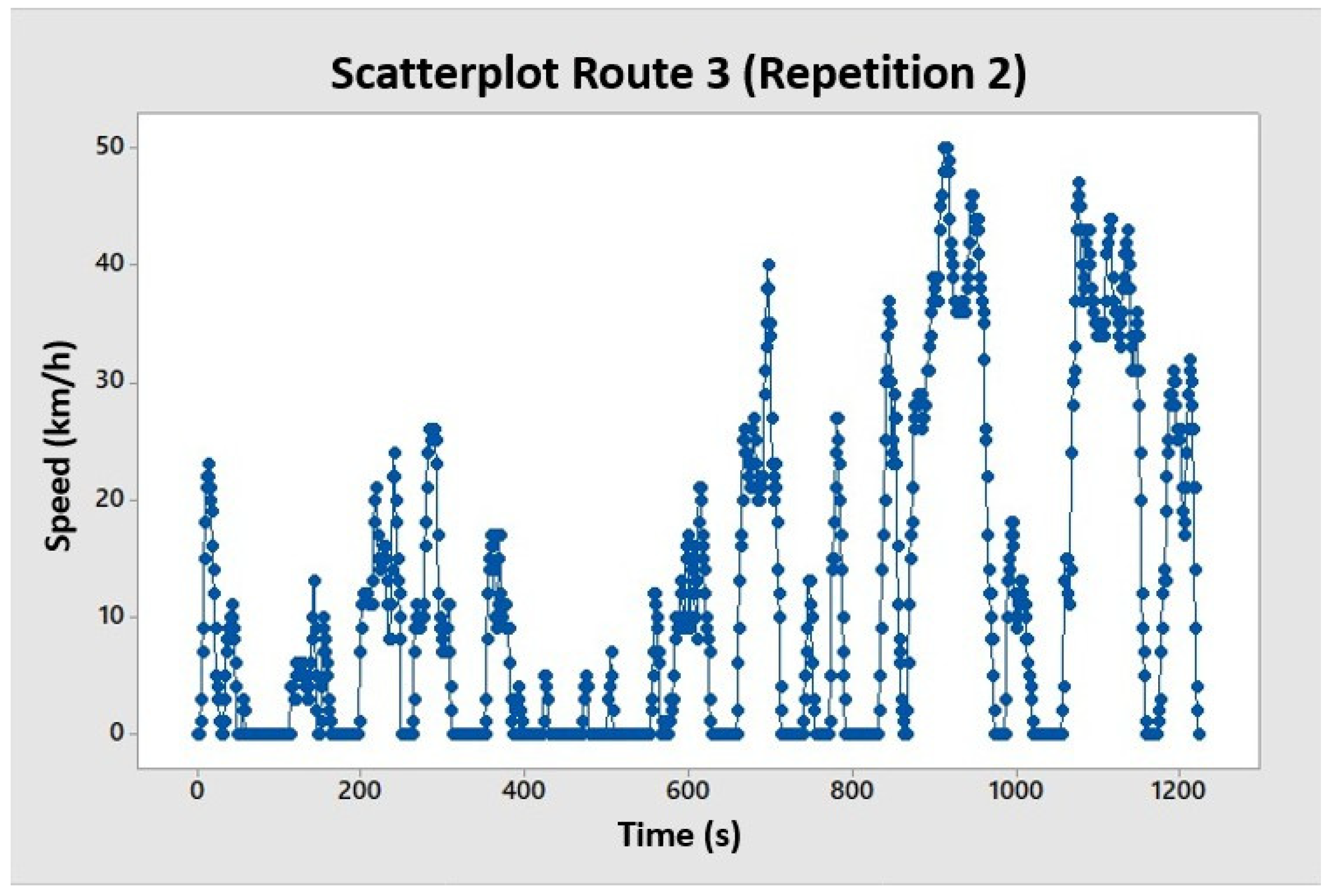
Figure A7.
Data obtained from the 11 repetitions of Route 4.
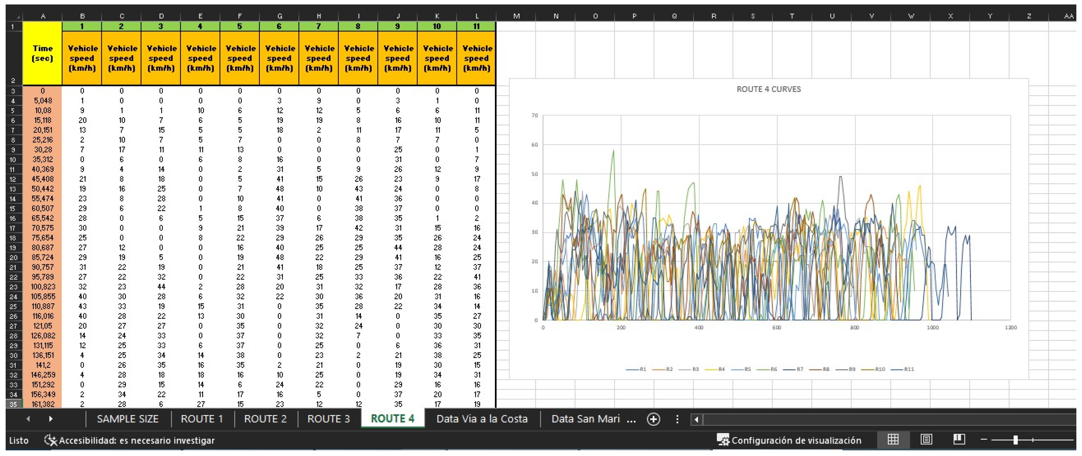
Figure A8.
Scatter plot of Route 4.
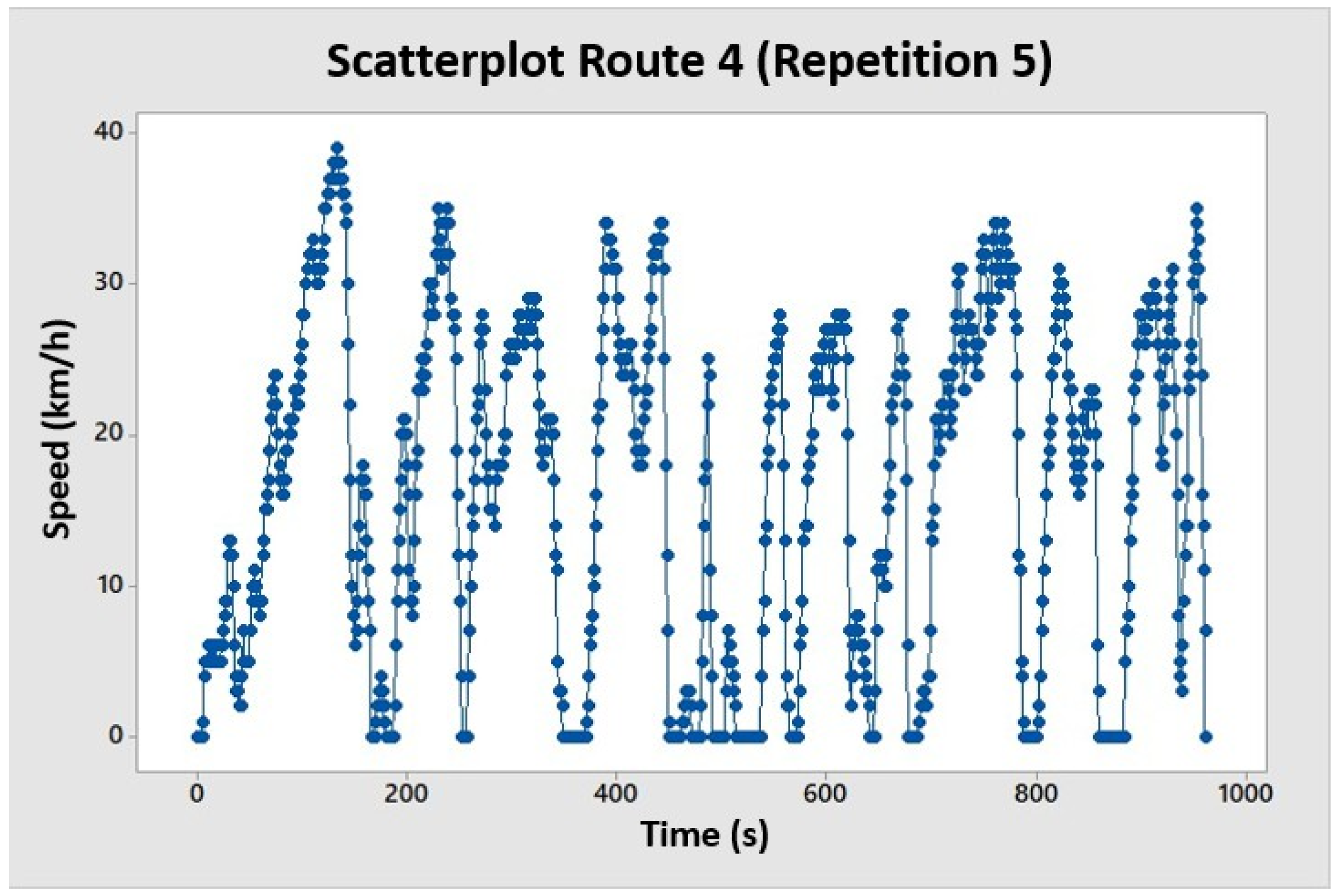
Figure A9.
Repetitions corresponding to Route 1 and its respective cycle.
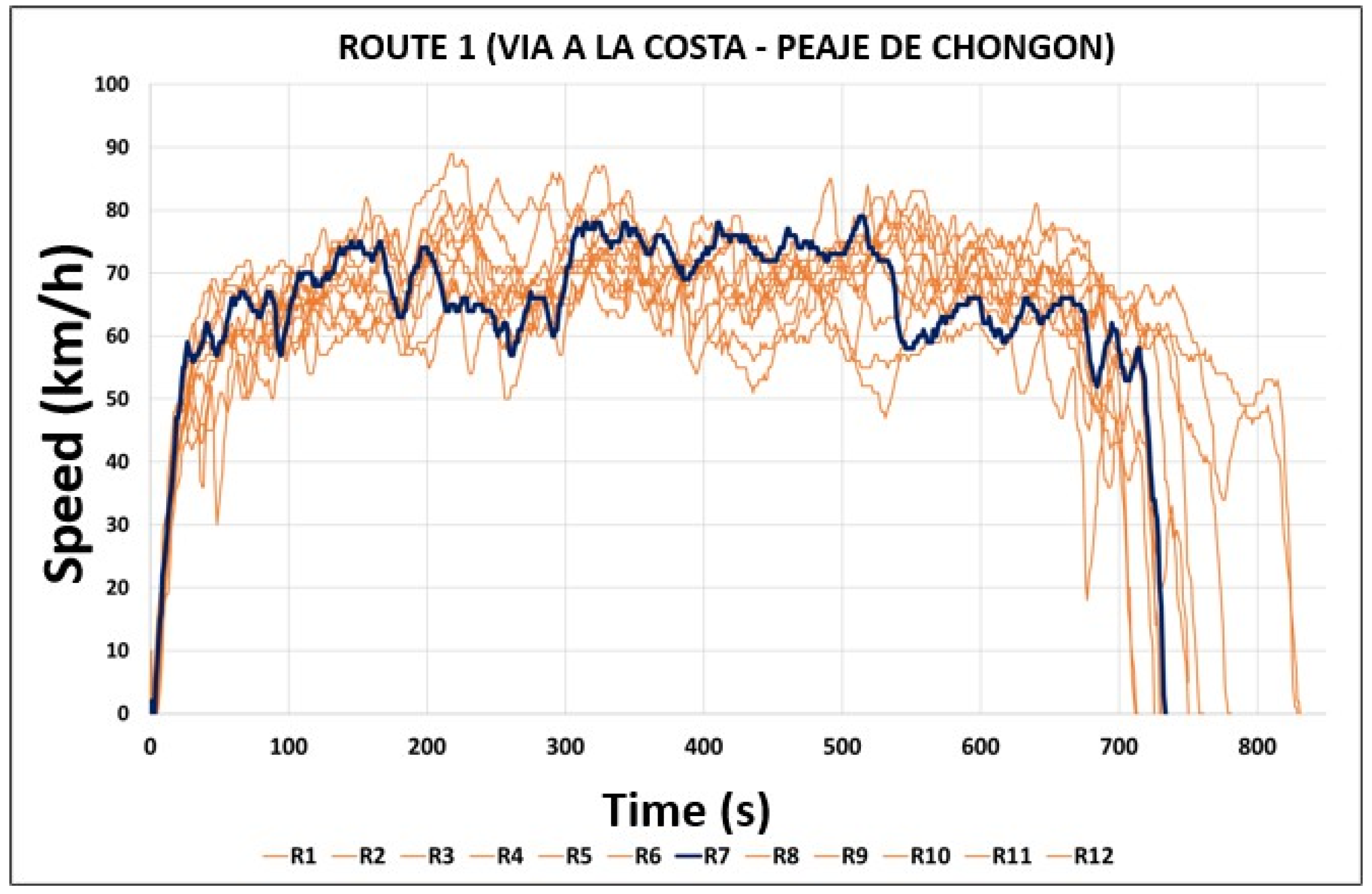
Figure A10.
Repetitions corresponding to Route 2 and its respective cycle.
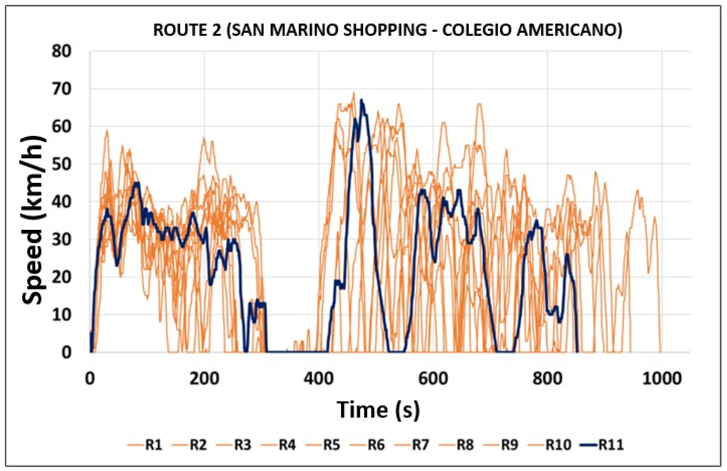
Figure A11.
Repetitions corresponding to Route 3 and its respective cycle.
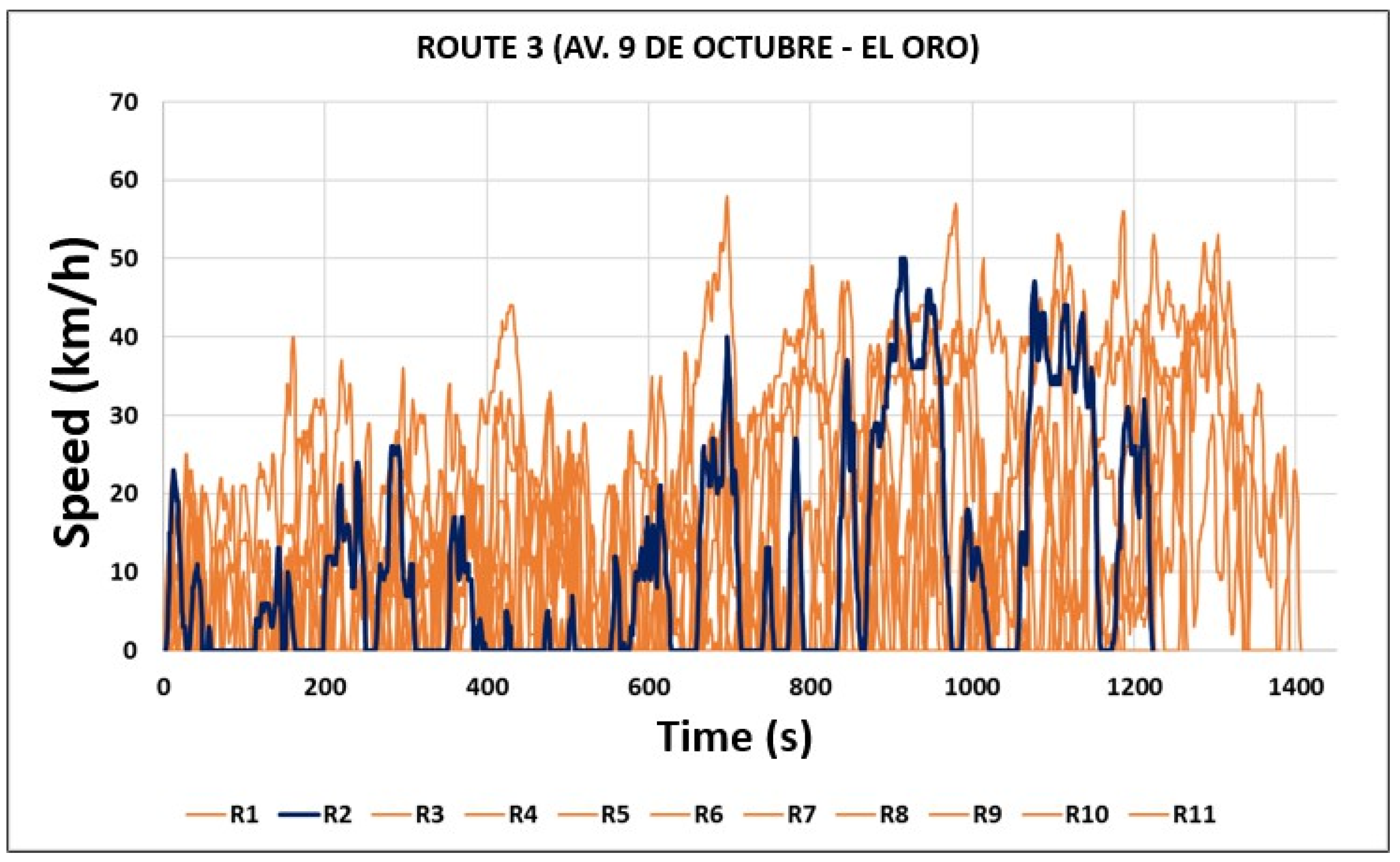
Figure A12.
Repetitions corresponding to Route 4 and its respective cycle.
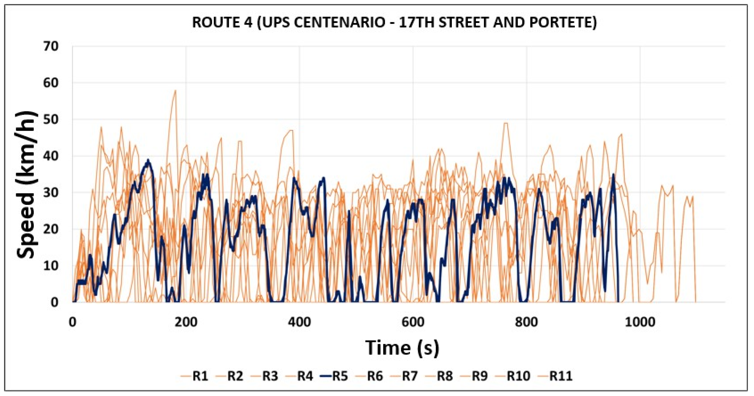
Figure A13.
Comparison: (a) Comparison of the FTP-75 cycle with Route 1 (Repetition n. 7). (b) Comparison of the FTP-75 cycle with Route 2 (Repetition n. 11). (c) Comparison of the FTP-75 cycle with Route 3 (Repetition n. 2). (d) Comparison of the FTP-75 cycle with Route 4 (Repetition n. 5).
Figure A13.
Comparison: (a) Comparison of the FTP-75 cycle with Route 1 (Repetition n. 7). (b) Comparison of the FTP-75 cycle with Route 2 (Repetition n. 11). (c) Comparison of the FTP-75 cycle with Route 3 (Repetition n. 2). (d) Comparison of the FTP-75 cycle with Route 4 (Repetition n. 5).
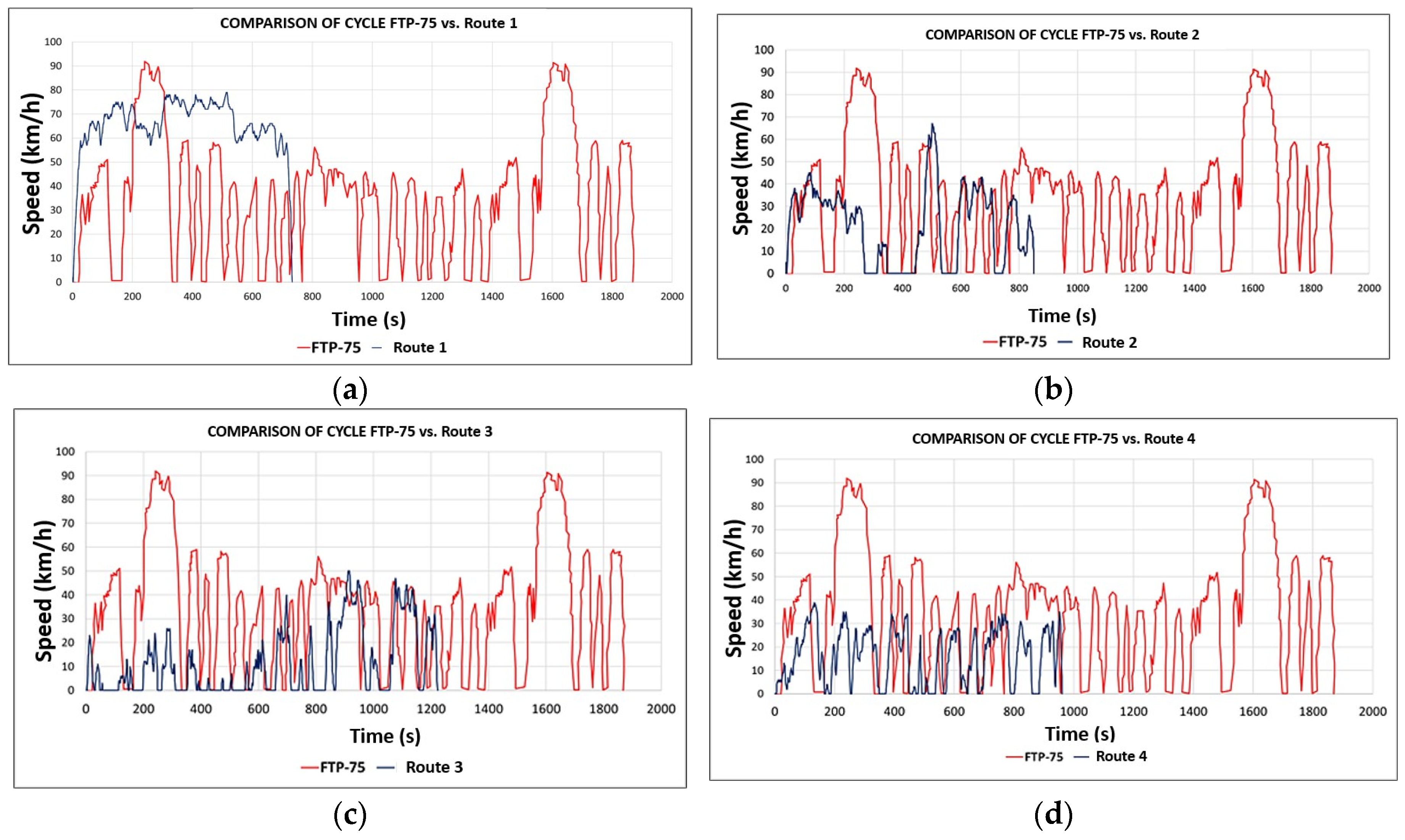
Figure A14.
Comparison: (a) Comparison of the NEDC cycle with Route 1 (Repetition n. 7). (b) Comparison of the NEDC cycle with Route 2 (Repetition n. 11). (c) Comparison of the NEDC cycle with Route 3 (Repetition n. 2). (d) Comparison of the NEDC cycle with Route 4 (Repetition n. 5).
Figure A14.
Comparison: (a) Comparison of the NEDC cycle with Route 1 (Repetition n. 7). (b) Comparison of the NEDC cycle with Route 2 (Repetition n. 11). (c) Comparison of the NEDC cycle with Route 3 (Repetition n. 2). (d) Comparison of the NEDC cycle with Route 4 (Repetition n. 5).
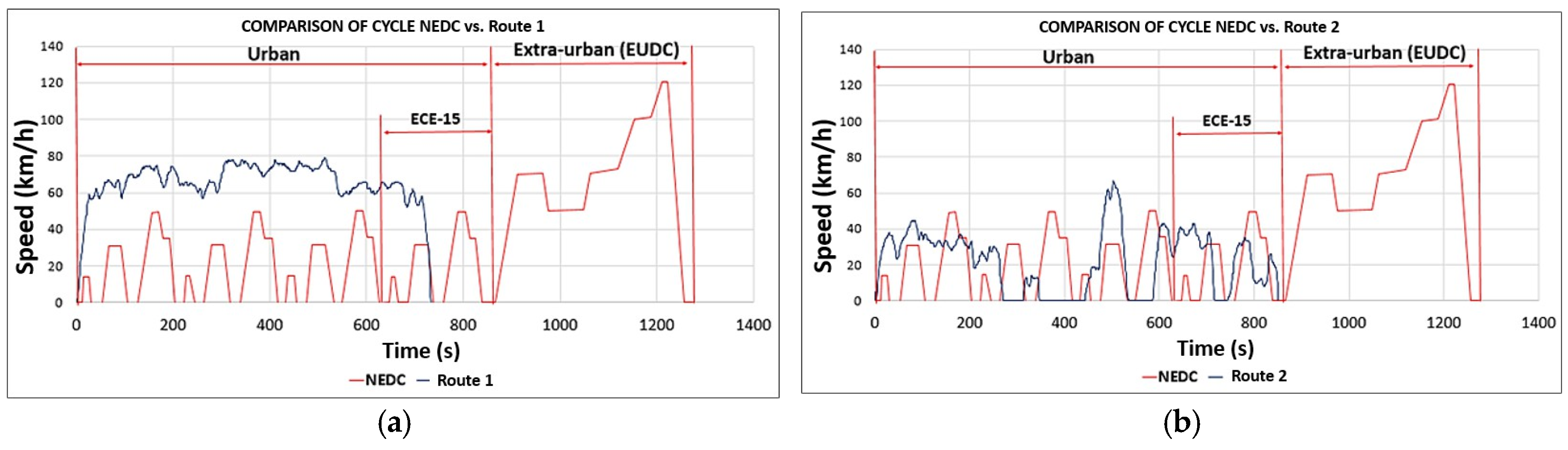
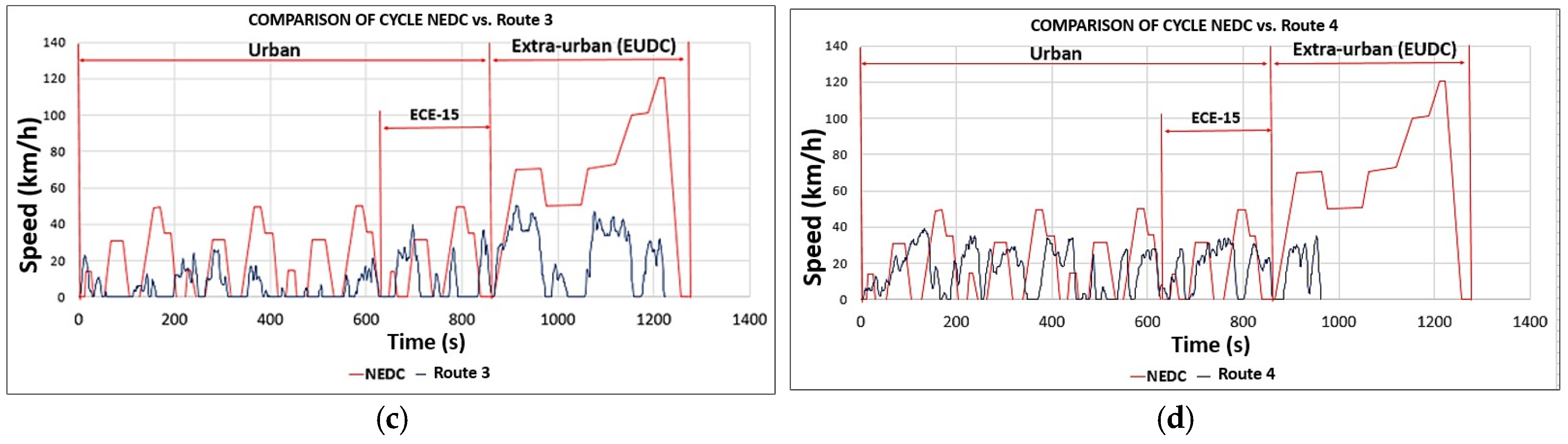
Figure A15.
Comparison of the EUDC cycle with Route 1 (Repetition n. 7).
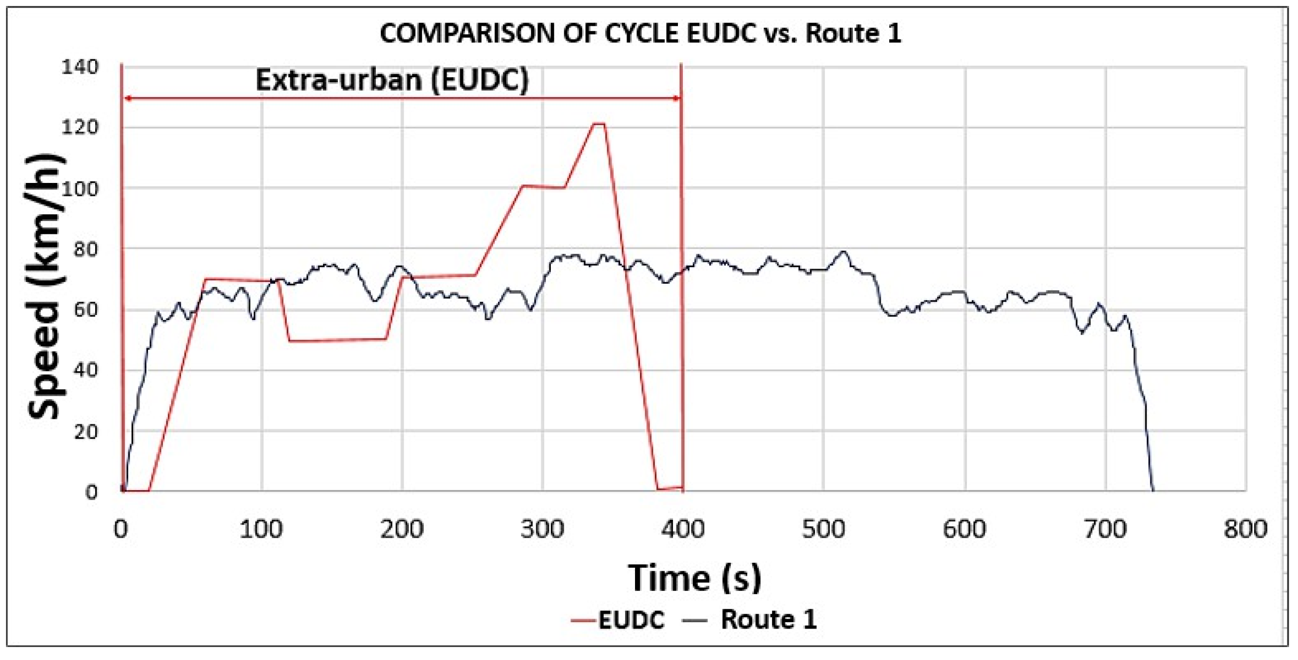
Figure A16.
Comparison of the HWFET cycle with Route 1 (Repetition n. 7).
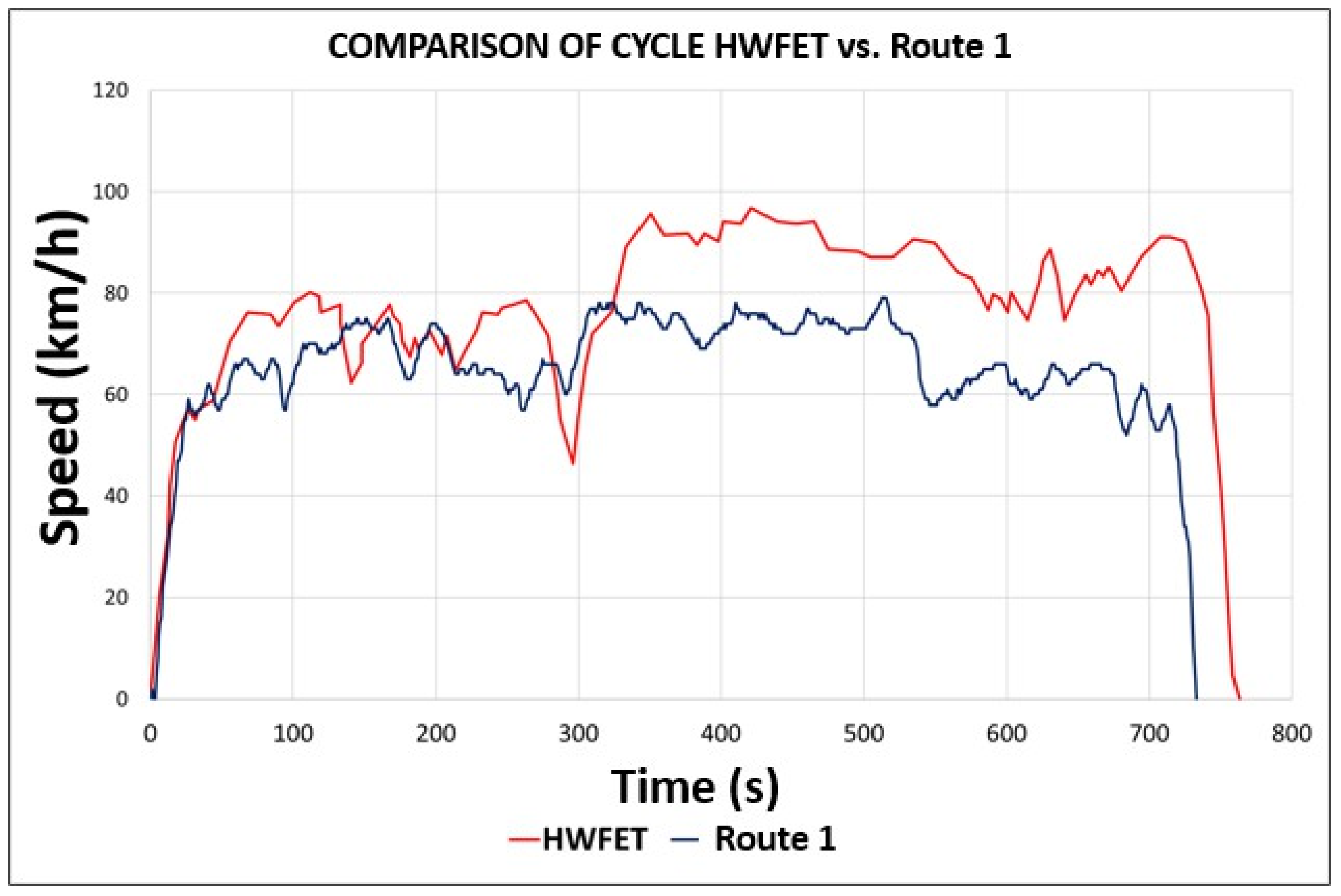
Figure A17.
Comparison of the ECE-15 cycle with Route 2 (Repetition n. 11).
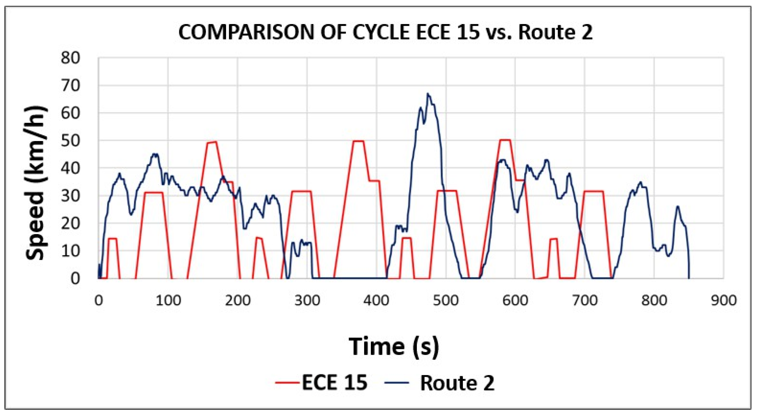
Figure A18.
Comparison of the WSL congested traffic cycle with Route 3 (Repetition n. 2).
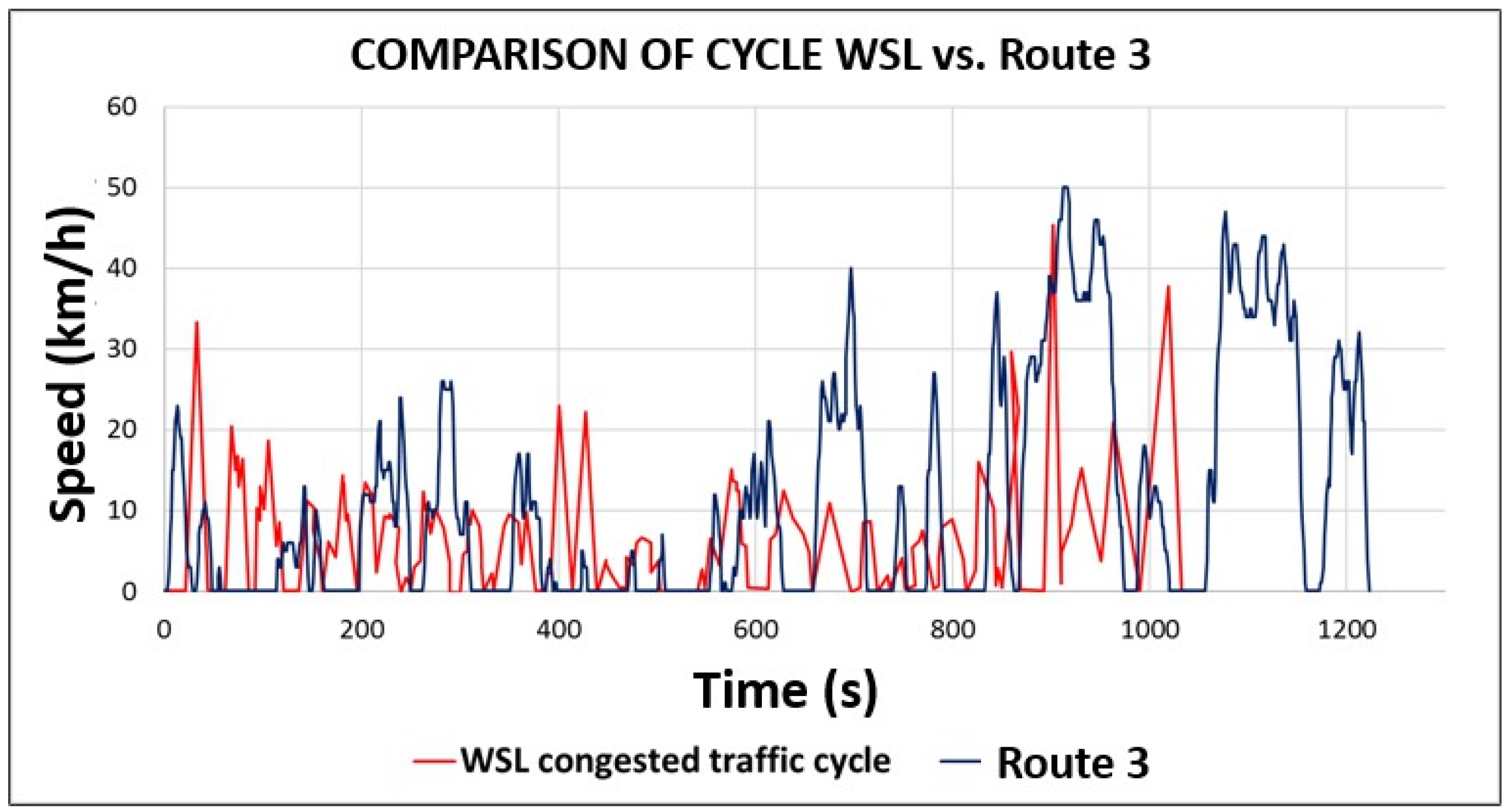
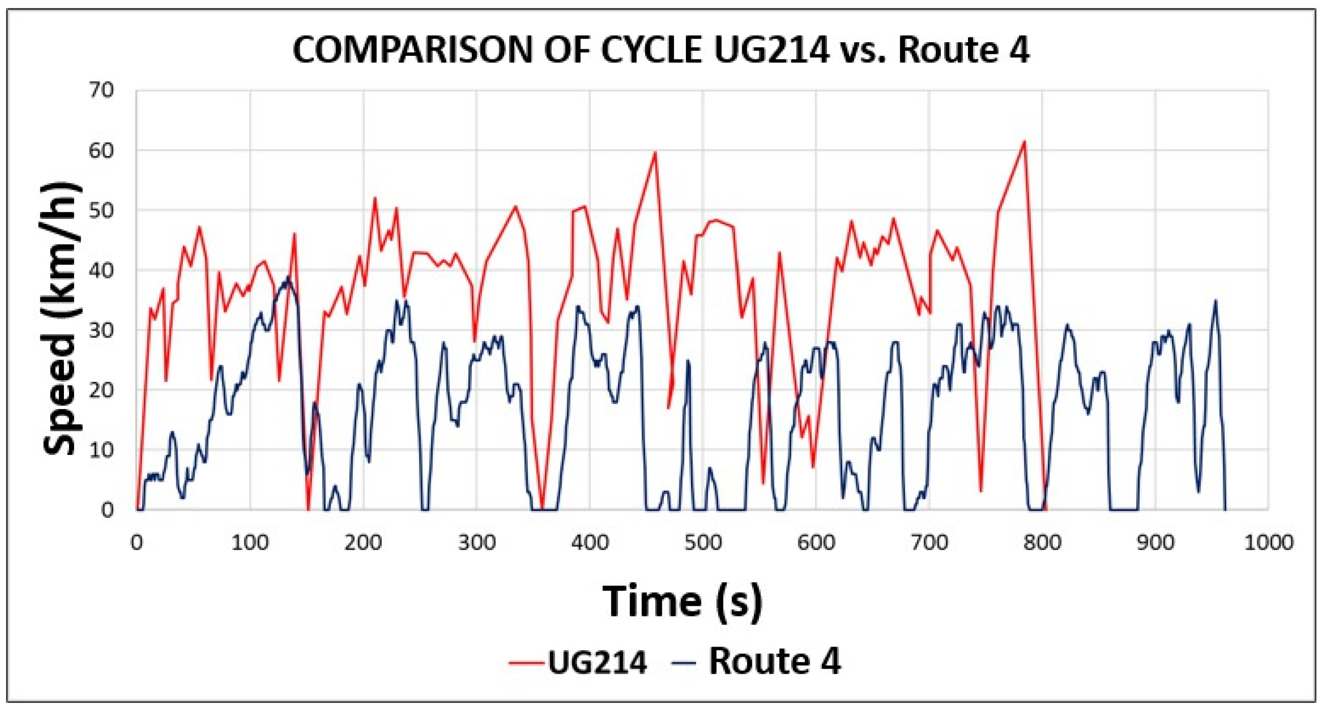
Figure A19.
Comparison of cycle UG214 with Route 4 (Repetition n. 5).
References
- Chauhan, B.P.; Joshi, G.J.; Parida, P. Development of candidate driving cycles for an urban arterial corridor of Vadodara city. Eur.Transp.-Trasp. Eur 2020, 4, 1–16. [Google Scholar]
- Lema, J. Emisiones y temperaturas de los gases de escape de un motor durante el arranque en frío aplicando dos tipos de combustibles. Polo del Conocimiento: Revista científico-profesional 2022, 7, 138–160. [Google Scholar]
- Serrano, L.; Santana, B.; Pires, N.; Correia, C. Performance, Emissions, and Efficiency of Biodiesel versus Hydrotreated Vegetable Oils (HVO), Considering Different Driving Cycles Sensitivity Analysis (NEDC and WLTP). Fuels 2021, 2, 448–470. [Google Scholar] [CrossRef]
- Leykun, M.G.; Mekonen, M.W. Investigation of the performance and emission characteristics of diesel engine fueled with biogas-diesel dual fuel. Fuels 2022, 3, 15–30. [Google Scholar] [CrossRef]
- Tong, H.Y.; Ng, K.W. Developing electric bus driving cycles with significant road gradient changes: A case study in Hong Kong. Sustainable Cities and Society 2023, 98, 104819. [Google Scholar] [CrossRef]
- Grüner, J.; Marker, S. A tool for generating individual driving cycles-IDCB. SAE International Journal of Commercial Vehicles 2016, 9, 417–428. [Google Scholar] [CrossRef]
- Gebisa, A.; Gebresenbet, G.; Gopal, R.; Nallamothu, R.B. Driving cycles for estimating vehicle emission levels and energy consumption. Future Transportation 2021, 1, 615–638. [Google Scholar] [CrossRef]
- Giraldo, M.; Huertas, J.I. Real emissions, driving patterns and fuel consumption of in-use diesel buses operating at high altitude. Transportation research part D: Transport and environment 2019, 77, 21–36. [Google Scholar] [CrossRef]
- Quiroga Villca, E. CICLOS DE CONDUCCIÓN EN LA PERSPECTIVA DE HOMOLOGACIÓN DEL VEHÍCULO EN PENDIENTE, CIUDAD DE LA PAZ-BOLIVIA. Revista Tecnológica 2023, 19, 1. [Google Scholar]
- Campaña, G.G.R.; Castro, E.H.G.; González, N.A.O. Evaluación del ciclo de operación en el transporte público de la Ciudad de Quito. Polo del Conocimiento 2024, 9, 4031–4055. [Google Scholar] [CrossRef]
- Salazar Sabas, O.A.; Quezada, B.E. Development of a driving cycle based on commercial vehicles and pollutant emissions. Revistainternacional de contaminación ambiental 2023, 39. [Google Scholar] [CrossRef]
- Zaragoza, C. Nuevos Ciclos de Conducción para Homologar Emisiones Contaminantes. Revista Tecnica de Centro Zaragosa 2018. [Google Scholar]
- Bagheri, E.; Masih-Tehrani, M.; Azadi, M.; Moosavian, A.; Sayegh, S.; Hakimollahi, M. Unveiling the impact of date-specific 534 analytics on vehicle fuel consumption and emissions: A case study of Shiraz city. Heliyon 2024, 10. [Google Scholar] [CrossRef]
- Mayakuntla, S.K.; Verma, A. A novel methodology for construction of driving cycles for Indian cities. Transportation research part D: transport and environment 2018, 65, 725–735. [Google Scholar] [CrossRef]
- Huzayyin, O.A.; Salem, H.; Hassan, M.A. A representative urban driving cycle for passenger vehicles to estimate fuel consumption and emission rates under real-world driving conditions. Urban Climate 2021, 36, 100810. [Google Scholar] [CrossRef]
- Guashpa, F.O.C.; Parrales, A.E.M.; Quiroz, W.V.P.; Ibarra, V.W.G. Determinación de un ciclo de conducción eficiente para la ciudad de Esmeraldas. Ciencia Latina Revista Científica Multidisciplinar 2023, 7, 1679–1691. [Google Scholar] [CrossRef]
- Llerena Viteri, D.R. Construcción del ciclo de conducción en la carretera Ambato-Riobamba; Technical report; Escuela Superior Politécnica de Chimborazo, 2022. [Google Scholar]
- Pérez Llanos, P.S.; Quito Sinchi, C.O. Determinación de los ciclos de conducción de un vehículo categoría M1 para la ciudad de Cuenca. B.S. thesis, Universidad Politécnica Salesiana, 2018. [Google Scholar]
- González-Oropeza, R. Los ciclos de manejo, una herramienta útil si es dinámica para evaluar el consumo de combustible y las emisiones contaminantes del auto transporte. Ingeniería, investigación y tecnología 2005, 6, 147–162. [Google Scholar]
- Guaillas Paqui, J.D.; Samaniego Marín, P.A. Determinación del ciclo real de conducción de un autobús de servicio urbano en la Ciudad de Loja para la evaluación de consumo de energía; Technical report; Escuela Superior Politécnica de Chimborazo, 2024. [Google Scholar]
- Giraldo, M.; Quirama, L.F.; Huertas, J.I.; Tibaquirá, J.E. The effect of driving cycle duration on its representativeness. World Electric Vehicle Journal 2021, 12, 212. [Google Scholar] [CrossRef]
- INEN. RTE INEN 2:1996 - EMISIONES DE VEHÍCULOS AUTOMOTORES Y MOTORES DE VEHÍCULOS USADOS. 1996. [Google Scholar]
- INEN. Inspección de Vehículos Automotores bajo Reglamentos Técnicos INEN. 2024. [Google Scholar]
- de Guayaquil, M. EVALUACIÓN SOCIOECONÓMICA. 2024. [Google Scholar]
- Pouresmaeili, M.A.; Aghayan, I.; Taghizadeh, S.A. Development of Mashhad driving cycle for passenger car to model vehicle exhaust emissions calibrated using on-board measurements. Sustainable cities and society 2018, 36, 12–20. [Google Scholar] [CrossRef]
- de Guayaquil, M. Solución vial 3 intersección Av. Juan Tanca Marengo con la Av. Rodrigo Chávez González y obras complementarias – programa CAF XVI. 2024. [Google Scholar]
- ATM. Rendición de Cuentas - INFORME 2023. 2023. [Google Scholar]
- Universo, E. Los horarios de mayor tráfico vehicular en Guayaquil y Samborondón. ATM 2022. [Google Scholar]
- ESPOL. El 23 El Universo. 2022. [Google Scholar]
- Universo, E. El área rural de expansión urbana en sector de vía a la costa abarca 1.193,6 hectáreas. Plan de Uso y Gestión del Suelo (PUGS) 2022. [Google Scholar]
- AEADE. Anuario 2023. 2023. [Google Scholar]
- MX+, O. OBDLink® MX Bluetooth. 2025. [Google Scholar]
- Visconti, P.; Rausa, G.; Del-Valle-Soto, C.; Velázquez, R.; Cafagna, D.; De Fazio, R. Innovative Driver Monitoring Systems and On-Board-Vehicle Devices in a Smart-Road Scenario Based on the Internet of Vehicle Paradigm: A Literature and Commercial Solutions Overview. Sensors 2025, 25, 562. [Google Scholar] [CrossRef] [PubMed]
- Rivera-Campoverde, N.D.; Arenas-Ramírez, B.; Muñoz Sanz, J.L.; Jiménez, E. GPS Data and Machine Learning Tools, a Practical and Cost-Effective Combination for Estimating Light Vehicle Emissions. Sensors 2024, 24, 2304. [Google Scholar] [CrossRef]
- Tocoronte, E.M.; Zuñiga, K.N.G.Z.G. Sofware minitab en la predicción del tiempo estándar. Sapientia Technological 2021, 2, 19. [Google Scholar]
- López-Chila, R.; Arteaga-Sotomayor, J.; Caballero-Barros, E.; Llerena-Izquierdo, J. An e-learning evaluation method with the effectiveness of the questionnaire tool in the VLEs. In Proceedings of the 2023 IEEE World Engineering Education Conference (EDUNINE); IEEE, 2023; pp. 1–6. [Google Scholar] [CrossRef]
- Valdéz, A. Desarrollo de Ciclos de Conducción Vehicular en el Municipio de Naucalpan. Edición Ún 2004. [Google Scholar]
- Quinchimbla Pisuña, F.E.; Solís Santamaría, J.M. Desarrollo de ciclos de conducción en ciudad, carretera y combinado para evaluar el rendimiento real del combustible de un vehículo con motor de ciclo Otto en el Distrito Metropolitano de Quito. Quito, 2017. [Google Scholar]
- Hyndman, R.J.; Athanasopoulos, G. Forecasting: principles and practice; OTexts, 2018. [Google Scholar]
- Tufte, E.R.; Graves-Morris, P.R. The visual display of quantitative information; Graphics press Cheshire, CT, 1983; Vol. 2. [Google Scholar]
- Few, S. Now you see it: simple visualization techniques for quantitative analysis; Analytics Press, 2009. [Google Scholar]
- López-Chila, R.; Sumba-Nacipucha, N.; Llerena-Izquierdo, J. Effectiveness of digital resources for cloned Linear Algebra courses at the undergraduate level. In Proceedings of the 2023 IEEE World Engineering Education Conference (EDUNINE). IEEE; 2023; pp. 1–5. [Google Scholar] [CrossRef]
- Barlow, T.J.; Latham, S.; McCrae, I.; Boulter, P. A reference book of driving cycles for use in the measurement of road vehicle emissions. TRL Published Project Report 2009. [Google Scholar]
Figure 1.
Routes: (a) Route 1, Via a la Costa-Peaje, 14.9 km long. (b) Route 2, San Marino-Colegio Americano with an extension of 5.7 km.
Figure 1.
Routes: (a) Route 1, Via a la Costa-Peaje, 14.9 km long. (b) Route 2, San Marino-Colegio Americano with an extension of 5.7 km.
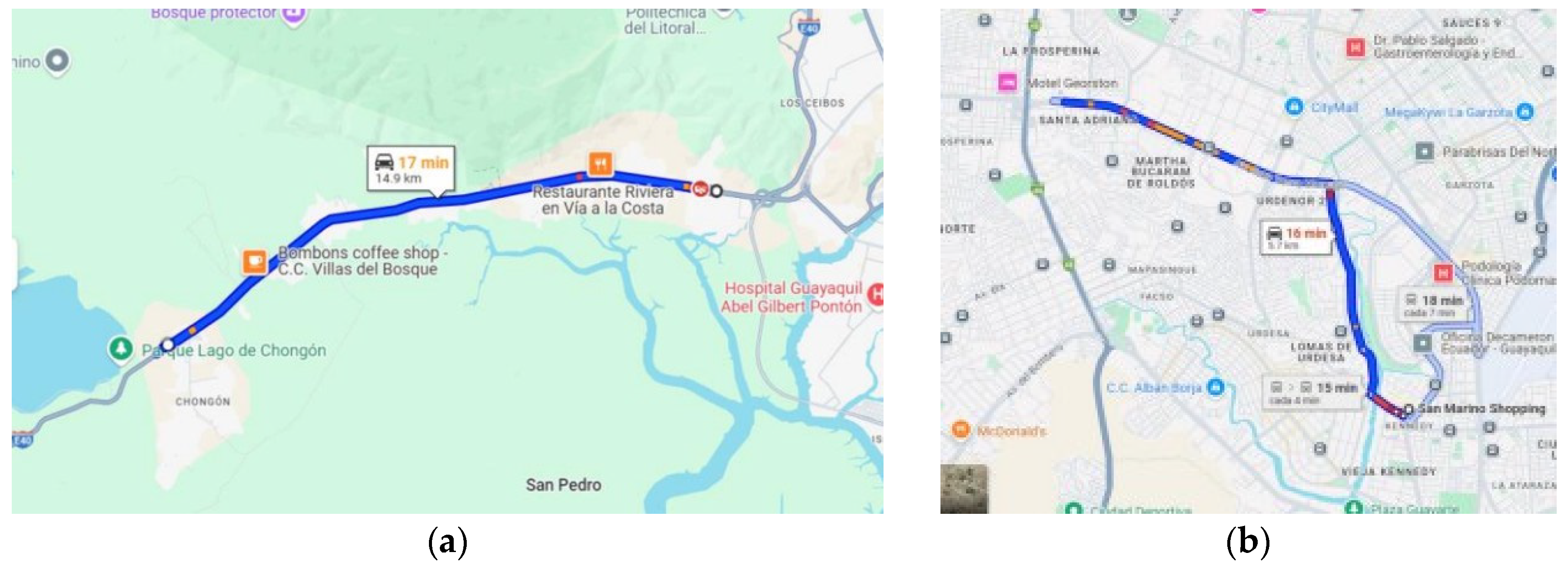
Figure 2.
Routes: (a) Route 3, UPS Centenario-17th Street and Portete with an extension of 4.7 km. (b) Route 4, Av. 9 de Octubre-El Oro with an extension of 3.9 km.
Figure 2.
Routes: (a) Route 3, UPS Centenario-17th Street and Portete with an extension of 4.7 km. (b) Route 4, Av. 9 de Octubre-El Oro with an extension of 3.9 km.
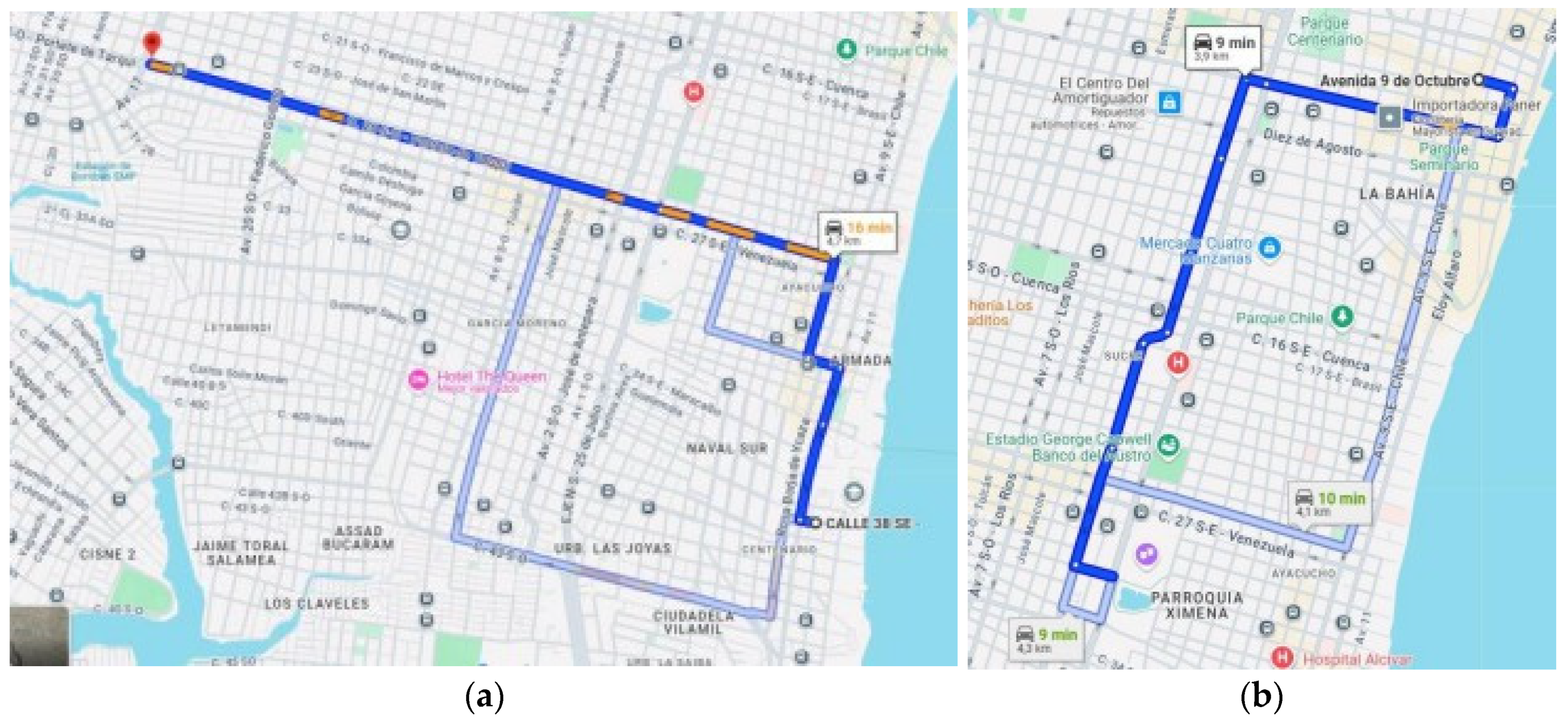
Figure 3.
Flow diagrams: (a) Process flow chart for data acquisition and driving cycle acquisition. (b) On-board instrumentation and device control.
Figure 3.
Flow diagrams: (a) Process flow chart for data acquisition and driving cycle acquisition. (b) On-board instrumentation and device control.
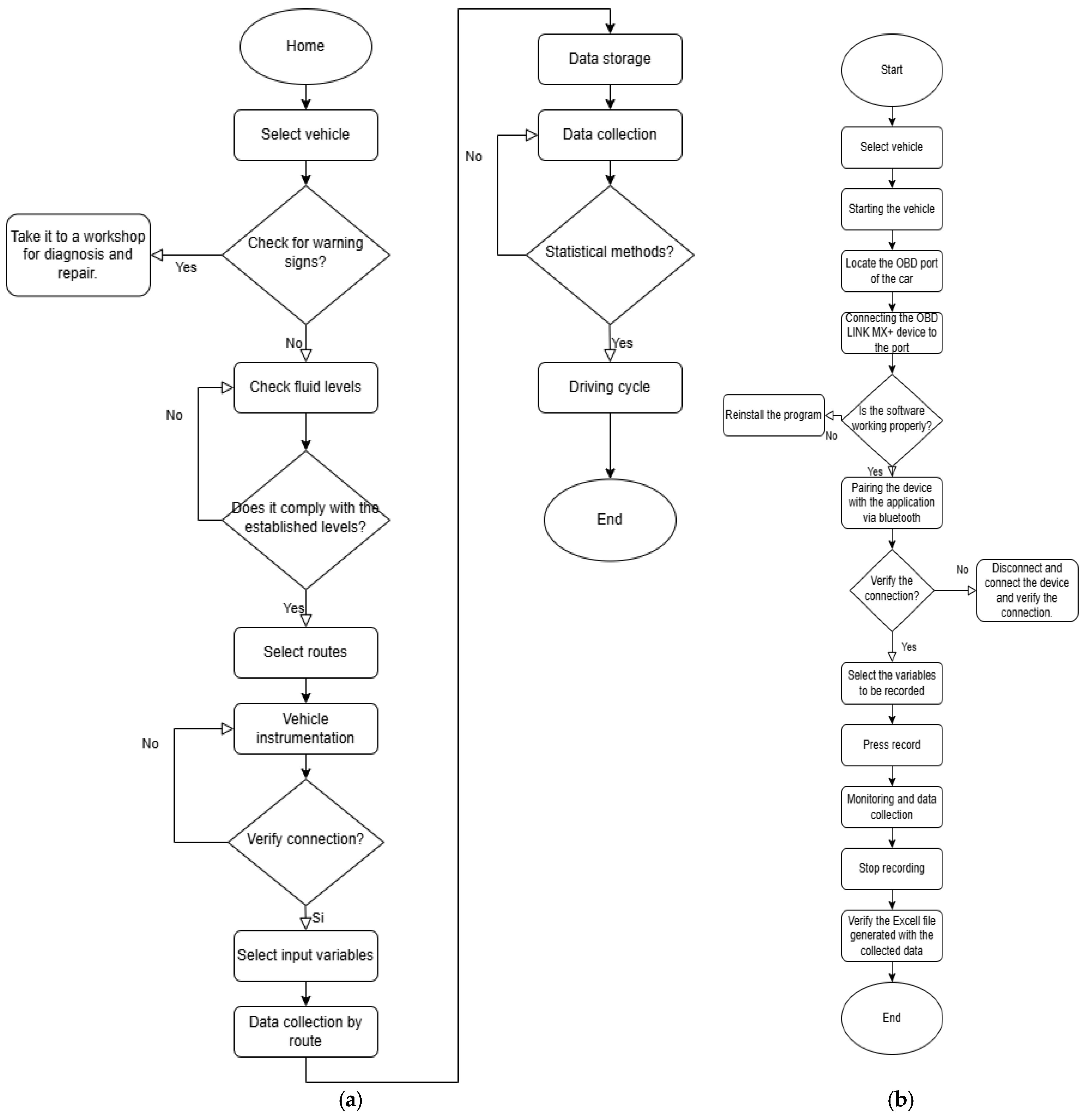
Figure 4.
Normality Test: (a) Route 1 does not follow a normal distribution in its data. (b) Route 2 does not follow a normal distribution in its data. (c) Route 3 does not follow a normal distribution in its data. (d) Route 4 does not follow a normal distribution in its data.
Figure 4.
Normality Test: (a) Route 1 does not follow a normal distribution in its data. (b) Route 2 does not follow a normal distribution in its data. (c) Route 3 does not follow a normal distribution in its data. (d) Route 4 does not follow a normal distribution in its data.
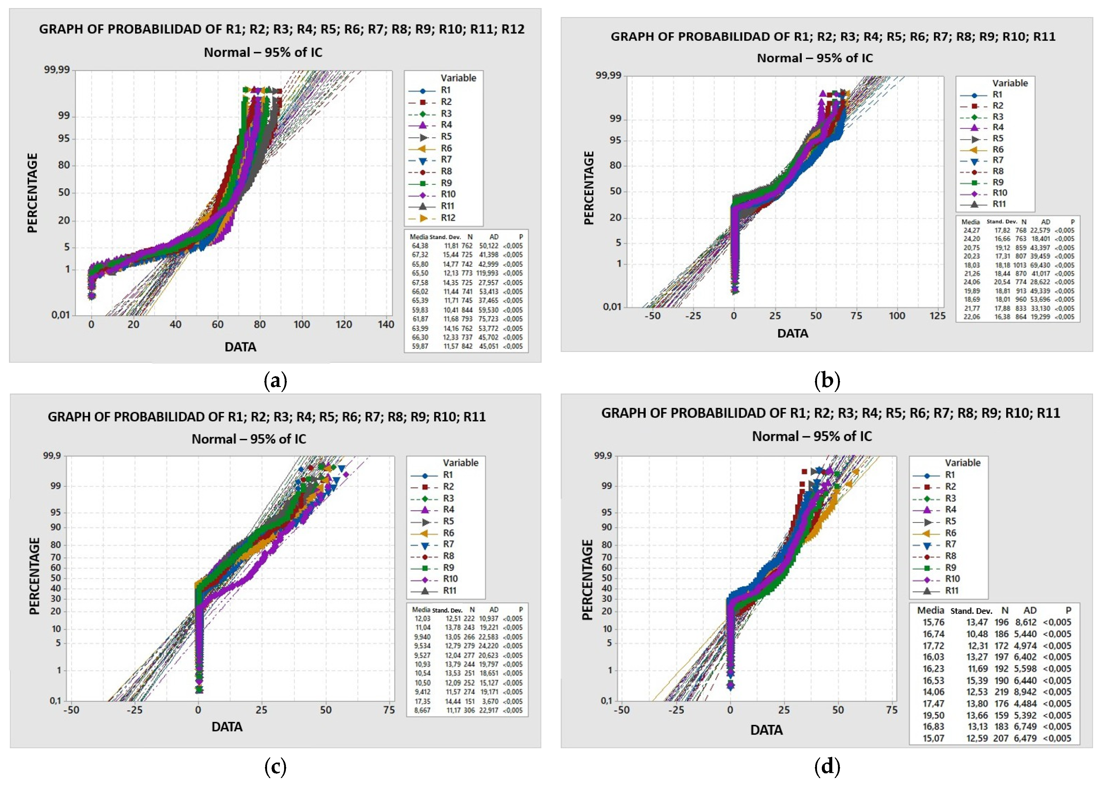
Figure 5.
Speed vs. Time Graph (Via a la Costa-Peaje).
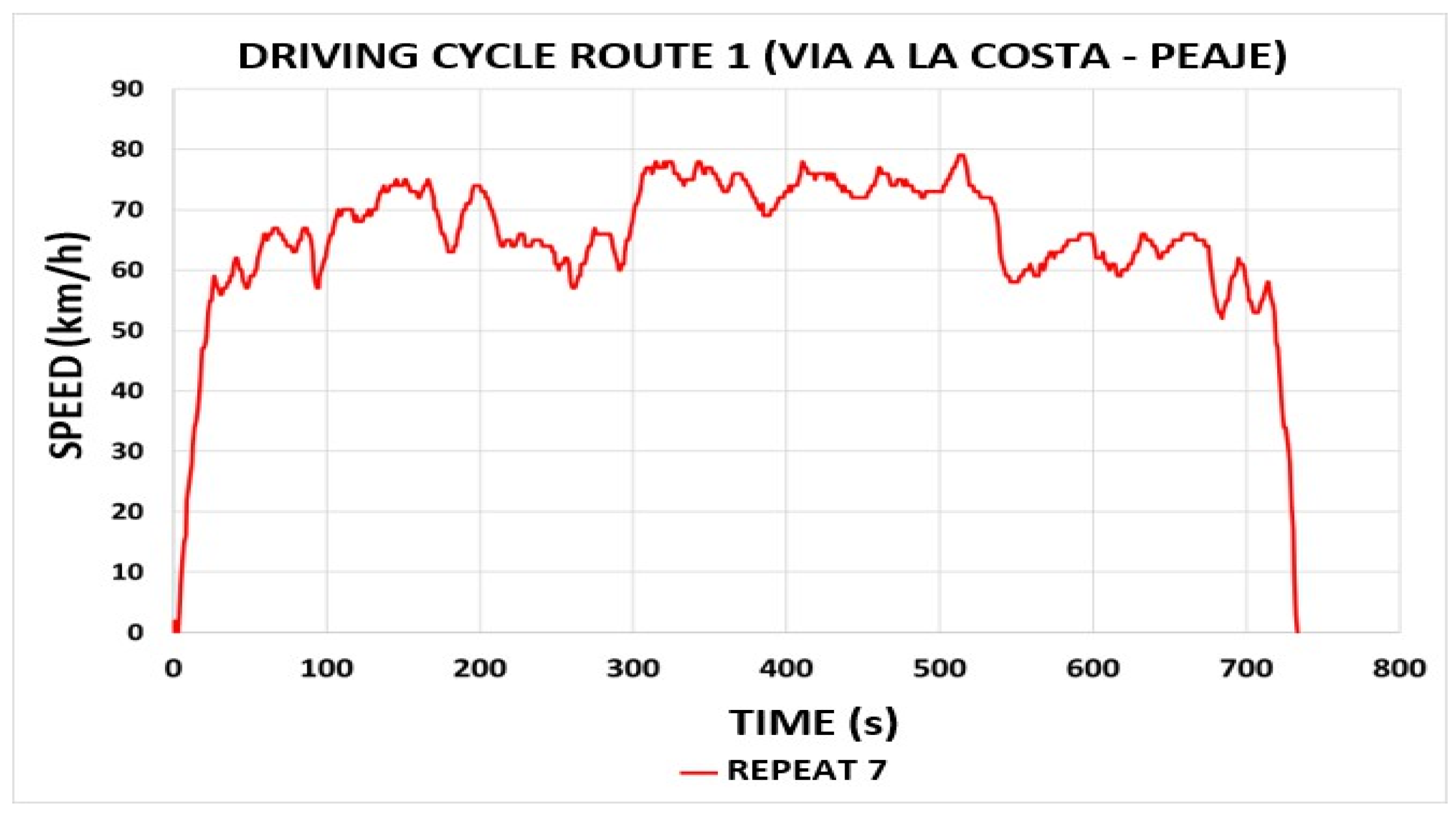
Figure 6.
Speed vs. Time Graph (San Marino-Colegio Americano).
| Average speed (km/h) | Max. speed (km/h) |
N | Driving time (s) | Idle time (s) | Distance (m) | Positive acceleration time (s) | % of driving time | % of time accelerating |
|---|---|---|---|---|---|---|---|---|
| 21,39 | 67 | 4 | 850,091 | 243 | 5712 | 306 | 71,41 | 36,00 |
Figure 7.
Speed vs. Time Graph (Av. 9 de Octubre-El Oro).
| Average speed (km/h) | Max. speed (km/h) |
N | Driving time (s) | Idle time (s) | Distance (m) | Positive acceleration time (s) | % of driving time | % of time accelerating |
|---|---|---|---|---|---|---|---|---|
| 11,05 | 50 | 18 | 1223,416 | 613 | 3900 | 332 | 49,89 | 27,14 |
| Average speed (km/h) | Max. speed (km/h) |
N | Driving time (s) | Idle time (s) | Distance (m) | Positive acceleration time (s) | % of driving time | % of time accelerating |
|---|---|---|---|---|---|---|---|---|
| 21,39 | 67 | 4 | 850,091 | 243 | 5712 | 306 | 71,41 | 36,00 |
Figure 8.
Speed vs. Time Graph (UPS Centenario-17th Street and Portete).
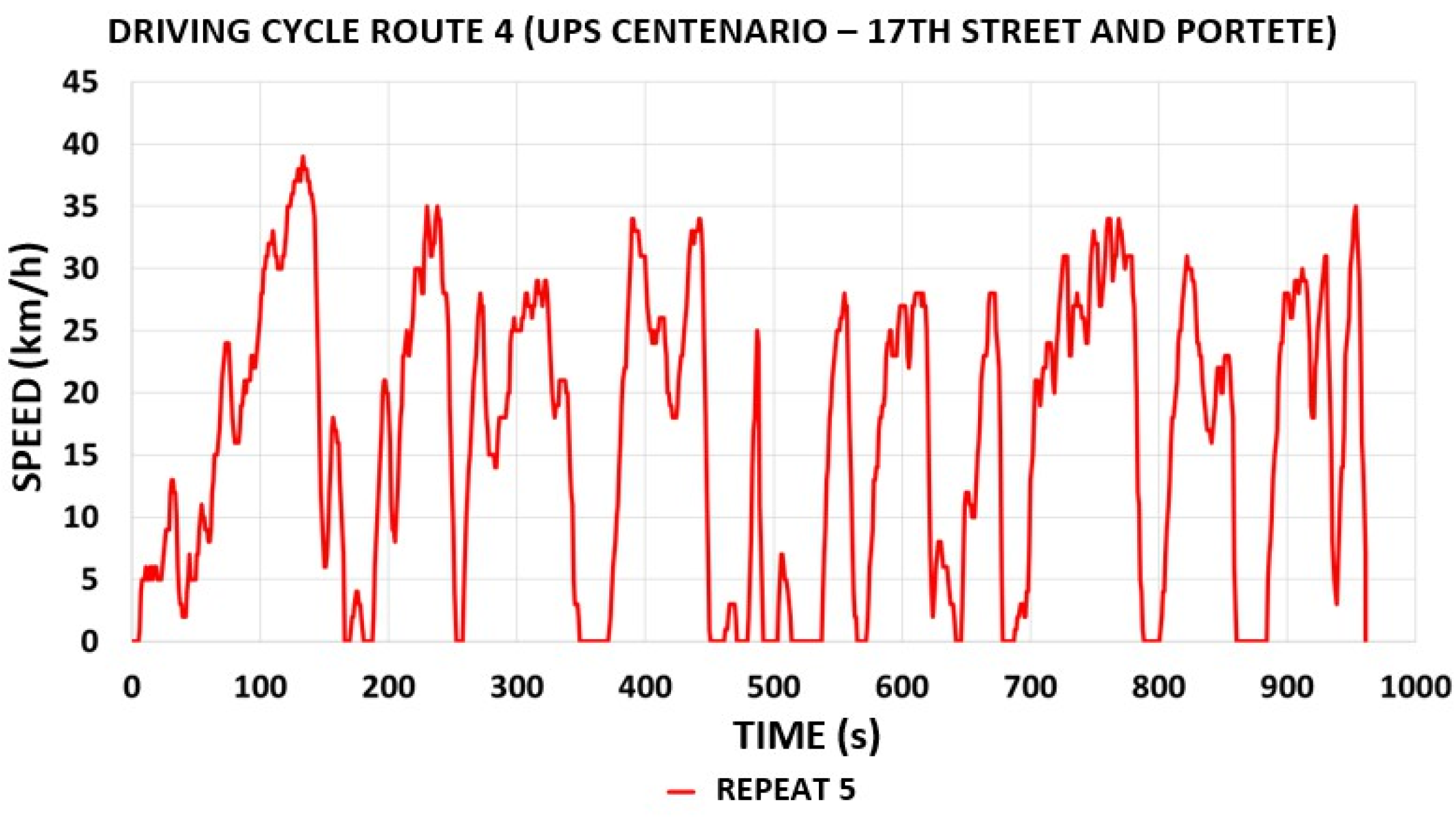
Table 1.
Technical specifications of the study vehicle.
| Vehicle Data | |
| Brand | Chevrolet |
| Model | Emotion |
| Year | 2015 |
| Fuel | Gasolina |
| Displacement | 4 cilindros, 1,8L |
| Type | DOCH 16V |
| Power | 103 Hp @ 6000 RPM |
| Torque | 144.1 Nm @ 3600 RPM |
Table 3.
Variables and their respective weightings in the study.
| Variables | Weightings (Wi) |
|---|---|
| Maximum speed (km/h) | 1 |
| Average speed (km/h) | 0.25 |
| Number of stops | 1 |
| Driving time (s) | 0.25 |
| Idle time (s) | 0.75 |
| Distance traveled (m) | 1 |
| Positive acceleration time (s) | 0.25 |
| % of driving time | 1 |
| % of time accelerating | 1 |
Table 4.
Average per route traveled.
| Tours | Routes | Distance (km) | Time (s) | Average Speed (km/h) |
|---|---|---|---|---|
| Vía a la Costa-Peaje | 1 | 14.9 | 777.139 | 63.94 |
| San Marino-Colegio Americano | 2 | 5.7 | 839.934 | 22.22 |
| Av. 9 de Octubre-El Oro | 3 | 3.9 | 1111.917 | 11.93 |
| UPS Centenario-17th Street and | 4 | 4.7 | 681.925 | 22.96 |
| Portete |
Table 5.
Sample size.
| Routes | Tours | Standard deviation | Standard error | Sample Size | Total number of repetitions |
|---|---|---|---|---|---|
| 1 | Vía a la Costa-Peaje | 18.45 | 0.617 | 1836 | 12 |
| 2 | San Marino-Colegio Americano | 17.87 | 0.643 | 1594 | 11 |
| 3 | Av. 9 de Octubre-El Oro | 13.527 | 0.402 | 2308 | 11 |
| 4 | UPS Centenario-17th Street and Portete | 15.48 | 0.585 | 1450 | 11 |
Table 6.
Data obtained from Route 1 (Via a la Costa-Peaje).
| R | Average speed (km/h) | Max. speed (km/h) |
N | Driving time (s) | Idle time (s) | Distance (m) | Positive acceleration time (s) | % of driving time | % of time accelerating |
|---|---|---|---|---|---|---|---|---|---|
| 1 | 64,38 | 79 | 0 | 750,54 | 5 | 14890 | 623 | 99,33 | 83,01 |
| 2 | 67,32 | 89 | 0 | 714,05 | 9 | 14899 | 565 | 98,74 | 79,13 |
| 3 | 65,80 | 83 | 0 | 730,50 | 11 | 14902 | 592 | 98,49 | 81,04 |
| 4 | 65,50 | 77 | 0 | 762,14 | 13 | 14911 | 588 | 98,29 | 77,15 |
| 5 | 67,58 | 87 | 0 | 713,81 | 12 | 14898 | 500 | 98,32 | 70,05 |
| 6 | 66,02 | 81 | 0 | 730,53 | 19 | 14904 | 553 | 97,40 | 75,70 |
| 7 | 65,39 | 79 | 0 | 735,62 | 10 | 14901 | 556 | 98,64 | 75,58 |
| 8 | 59,83 | 77 | 0 | 830,76 | 8 | 14897 | 667 | 99,04 | 80,29 |
| 9 | 61,87 | 73 | 0 | 781,19 | 7 | 14907 | 581 | 99,10 | 74,37 |
| 10 | 63,99 | 79 | 0 | 750,64 | 6 | 14888 | 566 | 99,20 | 75,40 |
| 11 | 66,30 | 84 | 0 | 725,00 | 13 | 14893 | 653 | 98,21 | 90,07 |
| 12 | 59,87 | 74 | 0 | 829,14 | 12 | 14896 | 665 | 98,55 | 80,20 |
Table 7.
Data obtained from Route 2 (San Marino-Colegio Americano).
| R | Average speed (km/h) | Max. speed (km/h) |
N | Driving time (s) | Idle time (s) | Distance (m) | Positive acceleration time (s) | % of driving time | % of time accelerating |
|---|---|---|---|---|---|---|---|---|---|
| 1 | 24,32 | 64 | 5 | 756,034 | 200 | 5691 | 277 | 73,55 | 36,64 |
| 2 | 24,20 | 58 | 6 | 751,015 | 149 | 5707 | 316 | 80,16 | 42,08 |
| 3 | 21,79 | 62 | 7 | 845,622 | 281 | 5699 | 317 | 66,77 | 37,49 |
| 4 | 20,70 | 54 | 5 | 882,628 | 262 | 5698 | 285 | 70,32 | 32,29 |
| 5 | 18,37 | 66 | 7 | 997,481 | 425 | 5710 | 313 | 57,39 | 31,38 |
| 6 | 21,29 | 69 | 7 | 855,873 | 305 | 5700 | 297 | 64,36 | 34,70 |
| 7 | 25,69 | 66 | 4 | 714,186 | 212 | 5711 | 247 | 70,32 | 34,58 |
| 8 | 20,40 | 66 | 8 | 898,316 | 331 | 5697 | 313 | 63,15 | 34,84 |
| 9 | 19,10 | 61 | 8 | 944,384 | 379 | 5690 | 301 | 59,87 | 31,87 |
| 10 | 22,03 | 62 | 4 | 819,683 | 249 | 5695 | 319 | 69,62 | 38,92 |
| 11 | 21,39 | 67 | 4 | 850,091 | 243 | 5712 | 306 | 71,41 | 36,00 |
Table 8.
Data obtained from Route 3 (Av. 9 de Octubre-El Oro).
| R | Average speed (km/h) | Max. speed (km/h) |
N | Driving time (s) | Idle time (s) | Distance (m) | Positive acceleration time (s) | % of driving time | % of time accelerating |
|---|---|---|---|---|---|---|---|---|---|
| 1 | 12,03 | 41 | 14 | 1118,043 | 417 | 3899 | 330 | 62,70 | 29,52 |
| 2 | 11,05 | 50 | 18 | 1223,416 | 613 | 3900 | 332 | 49,89 | 27,14 |
| 3 | 9,86 | 53 | 24 | 1349,582 | 676 | 3898 | 367 | 49,91 | 27,19 |
| 4 | 9,48 | 53 | 20 | 1407,603 | 758 | 3880 | 373 | 46,15 | 26,50 |
| 5 | 9,57 | 49 | 22 | 1391,487 | 701 | 3901 | 363 | 49,62 | 26,09 |
| 6 | 10,93 | 54 | 17 | 1229,422 | 638 | 3904 | 319 | 48,11 | 25,95 |
| 7 | 10,63 | 57 | 22 | 1260,551 | 607 | 3896 | 384 | 51,85 | 30,46 |
| 8 | 10,50 | 44 | 19 | 1265,836 | 558 | 3910 | 320 | 55,92 | 25,28 |
| 9 | 9,41 | 48 | 20 | 1380,757 | 689 | 3892 | 327 | 50,10 | 23,68 |
| 10 | 17,43 | 58 | 10 | 762,672 | 233 | 3895 | 290 | 69,45 | 38,02 |
| 11 | 11,24 | 47 | 16 | 1187,074 | 534 | 3901 | 311 | 55,02 | 26,20 |
Table 9.
Data obtained from Route 4 (UPS Centenario-17th Street and Portete).
| R | Average speed (km/h) | Maximum speed (km/h) |
N | Driving time (s) | Idle time (s) | Distance (m) | Positive acceleration time (s) | % of driving time | % of time accelerating |
|---|---|---|---|---|---|---|---|---|---|
| 1 | 15,76 | 43 | 13 | 988,19 | 345 | 4701 | 338 | 65,09 | 34,20 |
| 2 | 16,65 | 36 | 7 | 943,40 | 192 |
4700 | 566 | 79,65 | 60,00 |
| 3 | 17,71 | 44 | 10 | 873,02 | 217 | 4698 | 355 | 75,14 | 40,66 |
| 4 | 16,01 | 47 | 13 | 977,14 | 295 | 4692 | 352 | 69,81 | 36,02 |
| 5 | 16,27 | 39 | 11 | 961,22 | 247 | 4689 | 374 | 74,30 | 38,91 |
| 6 | 16,52 | 58 | 12 | 955,73 | 313 | 4711 | 287 | 67,25 | 30,03 |
| 7 | 14,17 | 41 | 16 | 1099,16 | 402 | 4694 | 371 | 63,43 | 33,75 |
| 8 | 17,50 | 45 | 8 | 886,64 | 229 | 4707 | 265 | 74,17 | 29,89 |
| 9 | 19,42 | 50 | 7 | 802,86 | 196 | 4699 | 253 | 75,59 | 31,51 |
| 10 | 17,03 | 46 | 10 | 918,60 | 249 | 4698 | 284 | 72,89 | 30,92 |
| 11 | 15,04 | 42 | 13 | 1040,42 | 331 | 4703 | 364 | 68,19 | 34,99 |
Table 10.
Statistical results of the data obtained in Route 1: Selected repetition number 7.
| Average speed (km/h) | Max. speed (km/h) |
N | Driving time (s) | Idle time (s) | Distance (m) | Positive acceleration time (s) | % of driving time | % of time accelerating | Total | ||
|---|---|---|---|---|---|---|---|---|---|---|---|
| W | 1 | 0,25 | 0,25 | 1 | 0,75 | 1 | 0,25 | 1 | 1 | 6,5 | |
| 65,45 | 79,00 | 0 | 743,08 | 10,50 | 14899 | 584,50 | 98,60 | 78,14 | |||
| 1 | 64,38 | 79 | 0 | 750,54 | 5 | 14890 | 623 | 99,33 | 83,01 | ||
| Y | 0,0025037 | 0,0000000 | 0 | 0,0015441 | 0,0604396 | 0,0000878 | 0,0025334 | 0,0011502 | 0,0095851 | 0,0778438 | |
| 2 | 67,32 | 89 | 0 | 714,05 | 9 | 14899 | 565 | 98,74 | 79,13 | ||
| Y | 0,0043932 | 0,0048685 | 0 | 0,0060101 | 0,0164835 | 0,0000052 | 0,0012831 | 0,0002230 | 0,0019436 | 0,0352103 | |
| 3 | 65,80 | 83 | 0 | 730,50 | 11 | 14902 | 592 | 98,49 | 81,04 | ||
| Y | 0,0008311 | 0,0019474 | 0 | 0,0026060 | 0,0054945 | 0,0000361 | 0,0004935 | 0,0001599 | 0,0057143 | 0,0172829 | |
| 4 | 65,50 | 77 | 0 | 762,14 | 13 | 14911 | 588 | 98,29 | 77,15 | ||
| Y | 0,0001262 | 0,0009737 | 0 | 0,0039451 | 0,0274725 | 0,0001291 | 0,0002303 | 0,0004718 | 0,0019436 | 0,0352923 | |
| 5 | 67,58 | 87 | 0 | 713,81 | 12 | 14898 | 500 | 98,32 | 70,05 | ||
| Y | 0,0050060 | 0,0038948 | 0 | 0,0060600 | 0,0164835 | 0,0000052 | 0,0055603 | 0,0004334 | 0,0159326 | 0,0533759 | |
| 6 | 66,02 | 81 | 0 | 730,53 | 19 | 14904 | 553 | 97,40 | 75,70 | ||
| Y | 0,0013444 | 0,0045249 | 0 | 0,0025983 | 0,0934066 | 0,0000568 | 0,0020728 | 0,0018685 | 0,0048048 | 0,1106772 | |
| 7 | 65,39 | 79 | 0 | 735,62 | 10 | 14901 | 556 | 98,64 | 75,58 | ||
| Y | 0,0001262 | 0,0000000 | 0 | 0,0015441 | 0,0054945 | 0,0000258 | 0,0018754 | 0,0000686 | 0,0050335 | 0,0141681 | |
| 8 | 59,83 | 77 | 0 | 830,76 | 8 | 14897 | 667 | 99,04 | 80,29 | ||
| Y | 0,0132136 | 0,0009737 | 0 | 0,0181529 | 0,0274725 | 0,0000155 | 0,0054287 | 0,0006871 | 0,0042315 | 0,0701756 | |
| 9 | 61,87 | 73 | 0 | 781,19 | 7 | 14907 | 581 | 99,10 | 74,37 | ||
| Y | 0,0084051 | 0,0029211 | 0 | 0,0078888 | 0,0384615 | 0,0000878 | 0,0002303 | 0,0007915 | 0,0074118 | 0,0661979 | |
| 10 | 63,99 | 79 | 0 | 750,64 | 6 | 14888 | 566 | 99,20 | 75,40 | ||
| Y | 0,0034230 | 0,0000000 | 0 | 0,0015642 | 0,0494505 | 0,0001084 | 0,0012173 | 0,0009425 | 0,0053869 | 0,0620928 | |
| 11 | 66,30 | 84 | 0 | 725,00 | 13 | 14893 | 653 | 98,21 | 90,07 | ||
| Y | 0,0020113 | 0,0024343 | 0 | 0,0037437 | 0,0274725 | 0,0000568 | 0,0045075 | 0,0006082 | 0,0234895 | 0,0643237 | |
| 12 | 59,87 | 74 | 0 | 829,14 | 12 | 14896 | 665 | 98,55 | 80,20 | ||
| Y | 0,0131029 | 0,0024343 | 0 | 0,0178166 | 0,0164835 | 0,0000258 | 0,0052971 | 0,0000686 | 0,0040662 | 0,0592951 |
Table 11.
Statistical results of the data obtained in Route 2: Selected repetition number 11.
| Average speed (km/h) | Max. speed (km/h) |
N | Driving time (s) | Idle time (s) | Distance (m) | Positive acceleration time (s) | % of driving time | % of time accelerating | Total | ||
|---|---|---|---|---|---|---|---|---|---|---|---|
| W | 1 | 0,25 | 0,25 | 1 | 0,75 | 1 | 0,25 | 1 | 1 | 6,5 | |
| 21,39 | 64,00 | 6 | 850,09 | 262,00 | 5699 | 306,00 | 69,62 | 34,84 | |||
| 1 | 24,32 | 64 | 5 | 756,034 | 200 | 5691 | 277 | 73,55 | 36,64 | ||
| Y | 0,0210822 | 0,0000000 | 0,006410 | 0,0170221 | 0,0273048 | 0,0002160 | 0,0036450 | 0,0086704 | 0,0079283 | 0,0922790 | |
| 2 | 24,20 | 58 | 6 | 751,015 | 149 | 5707 | 316 | 80,16 | 42,08 | ||
| Y | 0,0202616 | 0,0036058 | 0,000000 | 0,0179304 | 0,0497651 | 0,0002160 | 0,0012569 | 0,0232856 | 0,0319385 | 0,1482599 | |
| 3 | 21,79 | 62 | 7 | 845,622 | 281 | 5699 | 317 | 66,77 | 37,49 | ||
| Y | 0,0028959 | 0,0012019 | 0,006410 | 0,0008088 | 0,0083676 | 0,0000000 | 0,0013826 | 0,0063030 | 0,0116754 | 0,0390453 | |
| 4 | 20,70 | 54 | 5 | 882,628 | 262 | 5698 | 285 | 70,32 | 32,29 | ||
| Y | 0,0049146 | 0,0060096 | 0,006410 | 0,0058884 | 0,0000000 | 0,0000270 | 0,0026395 | 0,0015325 | 0,0112727 | 0,0386946 | |
| 5 | 18,37 | 66 | 7 | 997,481 | 425 | 5710 | 313 | 57,39 | 31,38 | ||
| Y | 0,0216879 | 0,0012019 | 0,006410 | 0,0266741 | 0,0717851 | 0,0002969 | 0,0008798 | 0,0270243 | 0,0152947 | 0,1712550 | |
| 6 | 21,29 | 69 | 7 | 855,873 | 305 | 5700 | 297 | 64,36 | 34,70 | ||
| Y | 0,0007106 | 0,0113122 | 0,006410 | 0,0010464 | 0,0189372 | 0,0000270 | 0,0011312 | 0,0116199 | 0,0006251 | 0,0518198 | |
| 7 | 25,69 | 66 | 4 | 714,186 | 212 | 5711 | 247 | 70,32 | 34,58 | ||
| Y | 0,0309813 | 0,0012019 | 0,012821 | 0,0245956 | 0,0220200 | 0,0003239 | 0,0074158 | 0,0015323 | 0,0011398 | 0,1020311 | |
| 8 | 20,40 | 66 | 8 | 898,316 | 331 | 5697 | 313 | 63,15 | 34,84 | ||
| Y | 0,0070766 | 0,0012019 | 0,012821 | 0,0087276 | 0,0303876 | 0,0000540 | 0,0008798 | 0,0142950 | 0,0000000 | 0,0754430 | |
| 9 | 19,10 | 61 | 8 | 944,384 | 379 | 5690 | 301 | 59,87 | 31,87 | ||
| Y | 0,0164608 | 0,0018029 | 0,012821 | 0,0170648 | 0,0515267 | 0,0002430 | 0,0006285 | 0,0215545 | 0,0131153 | 0,1352169 | |
| 10 | 22,03 | 62 | 4 | 819,683 | 249 | 5695 | 319 | 69,62 | 38,92 | ||
| Y | 0,0046427 | 0,0012019 | 0,012821 | 0,0055031 | 0,0057252 | 0,0001080 | 0,0016340 | 0,0000000 | 0,0179907 | 0,0496261 | |
| 11 | 21,39 | 67 | 4 | 850,091 | 243 | 5712 | 306 | 71,41 | 36,00 | ||
| Y | 0,0000000 | 0,0018029 | 0,012821 | 0,0000000 | 0,0083676 | 0,0003509 | 0,0000000 | 0,0039608 | 0,0050917 | 0,0323944 |
Table 12.
Statistical results of the data obtained in Route 3: Selected repetition number 2.
| Average speed (km/h) | Max. speed (km/h) |
N | Driving time (s) | Idle time (s) | Distance (m) | Positive acceleration time (s) | % of driving time | % of time accelerating | Total | ||
|---|---|---|---|---|---|---|---|---|---|---|---|
| W | 1 | 0,25 | 0,25 | 1 | 0,75 | 1 | 0,25 | 1 | 1 | 6,5 | |
| 10,63 | 50,00 | 19 | 1260,55 | 613,00 | 3899 | 330,00 | 50,10 | 26,50 | |||
| 1 | 12,03 | 41 | 14 | 1118,043 | 417 | 3899 | 330 | 62,70 | 29,52 | ||
| Y | 0,0201771 | 0,0069231 | 0,010121 | 0,0173926 | 0,0368930 | 0,0000000 | 0,0000000 | 0,0387007 | 0,0175154 | 0,1477233 | |
| 2 | 11,05 | 50 | 18 | 1223,416 | 613 | 3900 | 332 | 49,89 | 27,14 | ||
| Y | 0,0059718 | 0,0000000 | 0,002024 | 0,0045322 | 0,0000000 | 0,0000395 | 0,0002331 | 0,0006309 | 0,0037051 | 0,0171368 | |
| 3 | 9,86 | 53 | 24 | 1349,582 | 676 | 3898 | 367 | 49,91 | 27,19 | ||
| Y | 0,0112647 | 0,0023077 | 0,010121 | 0,0108659 | 0,0118585 | 0,0000395 | 0,0043124 | 0,0005817 | 0,0040330 | 0,0553847 | |
| 4 | 9,48 | 53 | 20 | 1407,603 | 758 | 3880 | 373 | 46,15 | 26,50 | ||
| Y | 0,0166430 | 0,0023077 | 0,002024 | 0,0179472 | 0,0272933 | 0,0007497 | 0,0050117 | 0,0121304 | 0,0000000 | 0,0841072 | |
| 5 | 9,57 | 49 | 22 | 1391,487 | 701 | 3901 | 363 | 49,62 | 26,09 | ||
| Y | 0,0153788 | 0,0007692 | 0,006073 | 0,0159803 | 0,0165642 | 0,0000789 | 0,0038462 | 0,0014666 | 0,0023905 | 0,0625476 | |
| 6 | 10,93 | 54 | 17 | 1229,422 | 638 | 3904 | 319 | 48,11 | 25,95 | ||
| Y | 0,0043224 | 0,0090498 | 0,004049 | 0,0037992 | 0,0047057 | 0,0001973 | 0,0012821 | 0,0061236 | 0,0032036 | 0,0367322 | |
| 7 | 10,63 | 57 | 22 | 1260,551 | 607 | 3896 | 384 | 51,85 | 30,46 | ||
| Y | 0,0000000 | 0,0053846 | 0,006073 | 0,0000000 | 0,0011294 | 0,0001184 | 0,0062937 | 0,0053635 | 0,0230135 | 0,0473760 | |
| 8 | 10,50 | 44 | 19 | 1265,836 | 558 | 3910 | 320 | 55,92 | 25,28 | ||
| Y | 0,0018949 | 0,0046154 | 0,000000 | 0,0006450 | 0,0103526 | 0,0004340 | 0,0011655 | 0,0178678 | 0,0070784 | 0,0440537 | |
| 9 | 9,41 | 48 | 20 | 1380,757 | 689 | 3892 | 327 | 50,10 | 23,68 | ||
| Y | 0,0176812 | 0,0015385 | 0,002024 | 0,0146708 | 0,0143054 | 0,0002762 | 0,0003497 | 0,0000000 | 0,0163507 | 0,0671966 | |
| 10 | 17,43 | 58 | 10 | 762,672 | 233 | 3895 | 290 | 69,45 | 38,02 | ||
| Y | 0,0983164 | 0,0061538 | 0,018219 | 0,0607645 | 0,0715272 | 0,0001578 | 0,0046620 | 0,0594188 | 0,0669127 | 0,3861319 | |
| 11 | 11,24 | 47 | 16 | 1187,074 | 534 | 3901 | 311 | 55,02 | 26,20 | ||
| Y | 0,0087657 | 0,0023077 | 0,006073 | 0,0089676 | 0,0148701 | 0,0000789 | 0,0022145 | 0,0150948 | 0,0017422 | 0,0601143 |
Table 13.
Statistical results of the data obtained in Route 4: Selected repetition number 5.
| Average speed (km/h) | Max. speed (km/h) |
N | Driving time (s) | Idle time (s) | Distance (m) | Positive acceleration time (s) | % of driving time | % of time accelerating | Total | ||
|---|---|---|---|---|---|---|---|---|---|---|---|
| W | 1 | 0,25 | 0,25 | 1 | 0,75 | 1 | 0,25 | 1 | 1 | 6,5 | |
| 16,52 | 44,00 | 11 | 955,73 | 249,00 | 4699 | 352,00 | 72,89 | 34,20 | |||
| 1 | 15,76 | 43 | 13 | 988,19 | 345 | 4701 | 338 | 65,09 | 34,20 | ||
| Y | 0,0070430 | 0,0008741 | 0,006993 | 0,0052255 | 0,0444856 | 0,0000655 | 0,0015297 | 0,0164744 | 0,0000000 | 0,0826908 | |
| 2 | 16,65 | 36 | 7 | 943,40 | 192 | 4700 | 566 | 79,65 | 60,00 | ||
| Y | 0,0012391 | 0,0069930 | 0,013986 | 0,0019846 | 0,0264133 | 0,0000327 | 0,0233829 | 0,0142561 | 0,1160094 | 0,2042973 | |
| 3 | 17,71 | 44 | 10 | 873,02 | 217 | 4698 | 355 | 75,14 | 40,66 | ||
| Y | 0,0110917 | 0,0000000 | 0,003497 | 0,0133139 | 0,0148285 | 0,0000327 | 0,0003278 | 0,0047495 | 0,0290544 | 0,0768950 | |
| 4 | 16,01 | 47 | 13 | 977,14 | 295 | 4692 | 352 | 69,81 | 36,02 | ||
| Y | 0,0046737 | 0,0026224 | 0,006993 | 0,0034461 | 0,0213160 | 0,0002292 | 0,0000000 | 0,0065082 | 0,0081848 | 0,0539734 | |
| 5 | 16,27 | 39 | 11 | 961,22 | 247 | 4689 | 374 | 74,30 | 38,91 | ||
| Y | 0,0022776 | 0,0043706 | 0,000000 | 0,0008844 | 0,0009268 | 0,0003274 | 0,0024038 | 0,0029762 | 0,0211620 | 0,0353288 | |
| 6 | 16,52 | 58 | 12 | 955,73 | 313 | 4711 | 287 | 67,25 | 30,03 | ||
| Y | 0,0000000 | 0,0316742 | 0,003497 | 0,0000000 | 0,0296571 | 0,0003929 | 0,0071023 | 0,0119105 | 0,0187764 | 0,1030099 | |
| 7 | 14,17 | 41 | 16 | 1099,16 | 402 | 4694 | 371 | 63,43 | 33,75 | ||
| Y | 0,0218351 | 0,0026224 | 0,017483 | 0,0230881 | 0,0708990 | 0,0001637 | 0,0020760 | 0,0199804 | 0,0020277 | 0,1601750 | |
| 8 | 17,50 | 45 | 8 | 886,64 | 229 | 4707 | 265 | 74,17 | 29,89 | ||
| Y | 0,0091915 | 0,0008741 | 0,010490 | 0,0111210 | 0,0092678 | 0,0002619 | 0,0095061 | 0,0026990 | 0,0194125 | 0,0728235 | |
| 9 | 19,42 | 50 | 7 | 802,86 | 196 | 4699 | 253 | 75,59 | 31,51 | ||
| Y | 0,0270389 | 0,0052448 | 0,013986 | 0,0246071 | 0,0245598 | 0,0000000 | 0,0108173 | 0,0056858 | 0,0121072 | 0,1240468 | |
| 10 | 17,03 | 46 | 10 | 918,60 | 249 | 4698 | 284 | 72,89 | 30,92 | ||
| Y | 0,0048295 | 0,0017483 | 0,003497 | 0,0059774 | 0,0000000 | 0,0000327 | 0,0074301 | 0,0000000 | 0,0147854 | 0,0382999 | |
| 11 | 15,04 | 42 | 13 | 1040,42 | 331 | 4703 | 364 | 68,19 | 34,99 | ||
| Y | 0,0137399 | 0,0017483 | 0,006993 | 0,0136328 | 0,0379981 | 0,0001310 | 0,0013112 | 0,0099355 | 0,0035173 | 0,0890070 |
Table 14.
Driving cycle parameters Route 1.
| Average speed (km/h) | Max. speed (km/h) |
N | Driving time (s) | Idle time (s) | Distance (m) | Positive acceleration time (s) | % of driving time | % of time accelerating |
|---|---|---|---|---|---|---|---|---|
| 65,39 | 79 | 0 | 735,62 | 10 | 14901 | 556 | 98,64 | 75,58 |
Table 15.
Driving cycle parameters Route 2.
| Average speed (km/h) | Max. speed (km/h) |
N | Driving time (s) | Idle time (s) | Distance (m) | Positive acceleration time (s) | % of driving time | % of time accelerating |
|---|---|---|---|---|---|---|---|---|
| 21,39 | 67 | 4 | 850,091 | 243 | 5712 | 306 | 71,41 | 36,00 |
Table 16.
Driving cycle parameters Route 3.
| Average speed (km/h) | Max. speed (km/h) |
N | Driving time (s) | Idle time (s) | Distance (m) | Positive acceleration time (s) | % of driving time | % of time accelerating |
|---|---|---|---|---|---|---|---|---|
| 11,05 | 50 | 18 | 1223,416 | 613 | 3900 | 332 | 49,89 | 27,14 |
Table 17.
Driving cycle parameters Route 4.
| Average speed (km/h) | Max. speed (km/h) |
N | Driving time (s) | Idle time (s) | Distance (m) | Positive acceleration time (s) | % of driving time | % of time accelerating |
|---|---|---|---|---|---|---|---|---|
| 16,27 | 39 | 11 | 961,22 | 247 | 4689 | 374 | 74,30 | 38,91 |
Table 18.
Comparison with other driving cycles.
| Variables | Guayaquil / Vía a la Costa | Guayaquil / San Marino | Guayaquil / Centro | Guayaquil / Portete | WSL Congested traffic cycle |
FTP-75 | HWFET | NEDC |
|---|---|---|---|---|---|---|---|---|
| Average speed (km/h) | 65,39 | 21,39 | 11,05 | 16,27 | 6,7 | 34,20 | 77,7 | 33,60 |
| Max. speed (km/h) | 79 | 67 | 50 | 39 | 43,65 | 91,09 | 96,32 | 120,09 |
| N | 0 | 4 | 18 | 11 | 22 | 16 | 0 | 14 |
| Time (s) | 735,624 | 850,091 | 1223,416 | 961,223 | 838 | 1633,00 | 764 | 939,00 |
| Idle Time (s) | 10 | 243 | 613 | 247 | 191 | 241 | 1 | 241 |
| Distance (m) | 14901 | 5712 | 3900 | 4689 | 1920,59 | 17786,59 | 16503,13 | 11016,63 |
| Positive acceleration time (s) | 556 | 306 | 332 | 374 | 314 | 683 | 264 | 278 |
| % of driving time | 98,64 | 71,41 | 49,89 | 74,3 | 81,44 | 87,14 | 99,87 | 79,58 |
| % of time accelerating | 75,58 | 36 | 27,14 | 38,91 | 30,52 | 36,45 | 34,51 | 23,56 |
Table 19.
Comparison with other driving cycles.
| Variables | Guayaquil / Via a la Costa | Guayaquil / San Marino | Guayaquil / Centro | Guayaquil / Portete | Cuenca | Quito / Ciudad | Quito / Autopista | Quito / Combined |
|---|---|---|---|---|---|---|---|---|
| Average speed (km/h) | 65,39 | 21,39 | 11,05 | 16,27 | 26,09 | 13,26 | 65,98 | 19,18 |
| Max. speed (km/h) | 79 | 67 | 50 | 39 | 61 | 45,77 | 89,91 | 78,32 |
| N | 0 | 4 | 18 | 11 | 12 | 58 | 2 | 63 |
| Time (s) | 735,624 | 850,091 | 1223,416 | 961,223 | 1168 | 3169,00 | 1493,00 | 2889,00 |
| Idle Time (s) | 10 | 243 | 613 | 247 | 280 | 1060 | 10 | 960 |
| Distance (m) | 14901 | 5712 | 3900 | 4689 | 10494 | 11914 | 27463 | 15673 |
| Positive acceleration time (s) | 556 | 306 | 332 | 374 | 530 | 1266 | 791 | 1036 |
| % of driving time | 98,64 | 71,41 | 49,89 | 74,3 | 81 | - | - | - |
| % of time accelerating | 75,58 | 36 | 27,14 | 38,91 | 36,6 | - | - | - |
Table 20.
Comparison with other driving cycles.
| Variables | Guayaquil / Via a la Costa | Guayaquil / San Marino | Guayaquil / Centro | Guayaquil / Portete | Esmeraldas | Ambato – Riobamba / Carretera | Ambato – Riobamba / Urban |
|---|---|---|---|---|---|---|---|
| Average speed (km/h) | 65,39 | 21,39 | 11,05 | 16,27 | 36,20 | 60,95 | 26,52 |
| Max. speed (km/h) | 79 | 67 | 50 | 39 | - | 120,40 | 63,40 |
| N | 0 | 4 | 18 | 11 | - | 2 | 13 |
| Time (s) | 735,624 | 850,091 | 1223,416 | 961,223 | 1750 | 2500 | 1300 |
| Idle Time (s) | 10 | 243 | 613 | 247 | - | - | - |
| Distance (m) | 14901 | 5712 | 3900 | 4689 | 15420 | - | - |
| Positive acceleration time (s) | 556 | 306 | 332 | 374 | - | - | - |
| % of driving time | 98,64 | 71,41 | 49,89 | 74,3 | - | 96,06 | 81,28 |
| % of time accelerating | 75,58 | 36 | 27,14 | 38,91 | - | - | - |
Disclaimer/Publisher’s Note: The statements, opinions and data contained in all publications are solely those of the individual author(s) and contributor(s) and not of MDPI and/or the editor(s). MDPI and/or the editor(s) disclaim responsibility for any injury to people or property resulting from any ideas, methods, instructions or products referred to in the content. |
© 2025 by the authors. Licensee MDPI, Basel, Switzerland. This article is an open access article distributed under the terms and conditions of the Creative Commons Attribution (CC BY) license (http://creativecommons.org/licenses/by/4.0/).
Copyright: This open access article is published under a Creative Commons CC BY 4.0 license, which permit the free download, distribution, and reuse, provided that the author and preprint are cited in any reuse.


