1. Introduction
The increase in pollutant emissions has been a problem over the last two decades, having a considerable impact on the environment, with 2019 statistics showing a record 36.7 billion metric tons of CO2, up from 23 billion tons at the beginning of the century [
1]. In the specific context of Ecuador, a 20.98% increase in CO2 emissions is reported for 2021 [
2]. Since the automotive industry is one of the main causes of pollutant emissions due to the burning of fossil fuels, it has become essential to reduce fuel consumption and consequently the pollutant emissions produced by vehicles [
3]. Thousands of cars circulate on the country’s streets every day; however, it must be taken into account that most of these cars are already very outdated. According to the National Institute of Statistics and Censuses (INEC), 28.1% of the total number of registered vehicles are more than twelve years old (2004 and earlier) [
4].
The Ecuadorian governmental regulations encourage the integration of more efficient technologies, in this context, hybrid vehicles would fulfil this purpose and the INEN RTE 017 standard can be used to evaluate exhaust emissions in Otto cycle vehicles [
5]. This is also a problem, as the user’s lack of knowledge about the qualities of the different driving modes in a hybrid vehicle, and even the technical data sheet does not determine a fuel consumption rate per driving mode in real conditions.
As such, the use of hybrid vehicles is a giant step towards zero-emission vehicles and their energy management is a key element for the development of new, more efficient technologies [
6]. With respect to the unexpected challenges faced by education in the pandemic era, hybrid vehicles seek to overcome obstacles by transitioning towards cleaner and more efficient mobility. Both scenarios demand reflection and adaptation to ensure a more sustainable future, and increased user awareness of hybrid vehicle driving modes will lead to the uptake of this technology [
7].
In consideration, the present study aims to analyze the influence of the driving modes of a hybrid vehicle during urban journeys in the city of Guayaquil, specifically to determine the rate of fuel consumption per kilometer travelled. The aim is to identify the factors that affect the fuel consumption of the Toyota Corolla Hybrid 2022, on defined urban routes in Guayaquil, by collecting real-time data using the OBD LINK MX+ tool. This data will be subjected to a detailed statistical analysis using Minitab software to understand fuel consumption behavior and its determinants in this specific context.
This study, carried out at the Salesian Polytechnic University during the period 2023 - 2024, is addressed not only to the academic community, providing a framework for future research, but also to owners and potential buyers of hybrid vehicles. It can also be seen as an innovative approach to effectively analyze performance and efficiency. By adapting quantitative empirical-analytical research methodology, it seeks to identify key patterns and trends in fuel consumption, thus establishing a solid basis for continuous improvement [
8]. It is hoped that the results obtained will be useful to better understand the performance, environmental and economic implications of this type of vehicle in the urban context of Guayaquil.
Likewise, the magazine International Sustainable Transportation [
10] analyzes consumption in a variety of driving styles, showing that in urban environments consumption is 13% lower and, on the highway, it is 34% higher in relation to the standard driving cycles of the U.S. Environmental Protection Agency (EPA). In 2020, the Cesar Vallejo University highlights in its comparative study on the road between a hybrid Sonata vehicle and a Yaris hatchback, consolidating the importance of efficiency in fuel consumption as it concludes that a hybrid vehicle can travel 36 km per gallon of fuel while the conventional one 37.5 km per gallon [
11].
By 2021, several similar studies will be carried out, such as the one by the Science of The Total Environment magazine [
12], which delved into the difference in consumption between hybrid and conventional vehicles, concluding that the former achieve significant savings. On the other hand, the World Electric Vehicle Journal investigates the impact of extremely low temperatures on fuel consumption, revealing a significant increase of 73% compared to consumption at room temperature [
13].
At the same time, the University of Ruse in Bulgaria [
14] explores the discrepancies between the actual consumption and the manufacturer’s specifications of a Toyota Yaris vehicle, obtaining as a result that the fuel consumption is significantly higher than the data sheet, being between (61.3-119.4) % in conventional mode and (35.4-74.2) % in Eco mode. Romero’s analysis in 2022 [
15] delves into the consumption in economy and sport modes, for which several factors are selected for the evaluation of analysis, among which were included driving mode, routes, constant driving, cruising speed and technical factors, highlighting the advantages of ECO mode in urban driving in terms of fuel economy.
2. Materials and Methods
Descriptive research and a Pearson correlation analysis were carried out to determine the factors that influence the study, due to the systematic approach used in the observation and recording of data, in order to establish relationships and patterns between the data collected to analyze the influence of driving modes in hybrid vehicles and determine the fuel rate per kilometer traveled and with a cross-sectional temporality. In addition, the approach was quantitative, due to the use of statistical techniques to measure, describe and explain fuel consumption in the vehicle, focusing the conclusions on an objective analysis [
16].
2.1. Data Collection Methods and Techniques Used
2.1.1. Description of the Study Area
The research was carried out in the city of Guayaquil, located in the coastal region of Ecuador. With a population of over 2.7 million inhabitants and a territorial extension of approximately 380 square kilometers [
17]. The average altitude of Guayaquil is around 4 meters above sea level, maintaining a predominantly tropical climate. To ensure the integrity of the data collected, specific routes were identified and defined within the urban area of Guayaquil, considering the points with the highest vehicular congestion. These routes were designed to cover different areas of the city and times of high traffic, thus ensuring a wide coverage of urban scenarios with a total of 6 routes.
According to the bibliographic compilation carried out in this study, it is focused on vehicular congestion, where the points of greatest traffic in the city of Guayaquil were determined. From this, 5 critical points were determined. Francisco de Orellana Avenue, which is classified as a commercial and service corridor, is a highly frequented road artery. In addition, at its specific intersection with José Santiago Castillo Street with a level of service type E, i.e., near or at its capacity limit, consequently, speed is reduced but uniform, freedom of maneuver is complex and comfort levels are low [
18].
Finally, according to a study published in the magazine Gaceta Técnica [
19], the critical points of vehicular congestion in the city of Guayaquil were identified, among which are; The historic center, where there is a high concentration of traffic due to its narrow streets and the presence of pedestrians attracted by stores, banks, offices, and government buildings, and the Avenida de las Américas, which is one of the city’s main thoroughfares connecting downtown with the northern part of Guayaquil but congested by the convergence of vehicles entering or leaving the city, and the Rafael Mendoza Avilés bridge, which connects the city of Guayaquil with the cantons of Eloy Alfaro and Samborondón, which is in high demand due to work and school activities.
Finally, according to a study published in the magazine Gaceta Técnica [
19], critical points of traffic congestion in the city of Guayaquil were identified, among which are; the historic center, which generates a high concentration of traffic due to its narrow streets and the presence of pedestrians attracted by stores, banks, offices and government buildings, the Avenida de las Américas, which is one of the main arteries of the city, and the Avenida de las Américas, which is one of the main arteries of the city, which is one of the city’s main thoroughfares connecting downtown with the northern part of Guayaquil but congested by the convergence of vehicles entering or leaving the city, and the Rafael Mendoza Avilés bridge, which connects the city of Guayaquil with the cantons of Eloy Alfaro and Samborondón, where there is high demand due to work and school activities.
Therefore, the critical points were identified and two hours of peak traffic were determined according to the Municipal Traffic Agency (ATM), which are between 06:00 and 09:00 and from 17:00 to 20:00, in the different streets of the city, this with the help of Google Maps, which has a function to analyze daily traffic in specific areas and times, the newspaper El Universo [
20], uses this tool and together with interviews presented results of peak hours in specific areas of the north, west, south and center of the city. These were used in this research to define 6 routes of analysis and the time at which it was suggested to perform different tests.
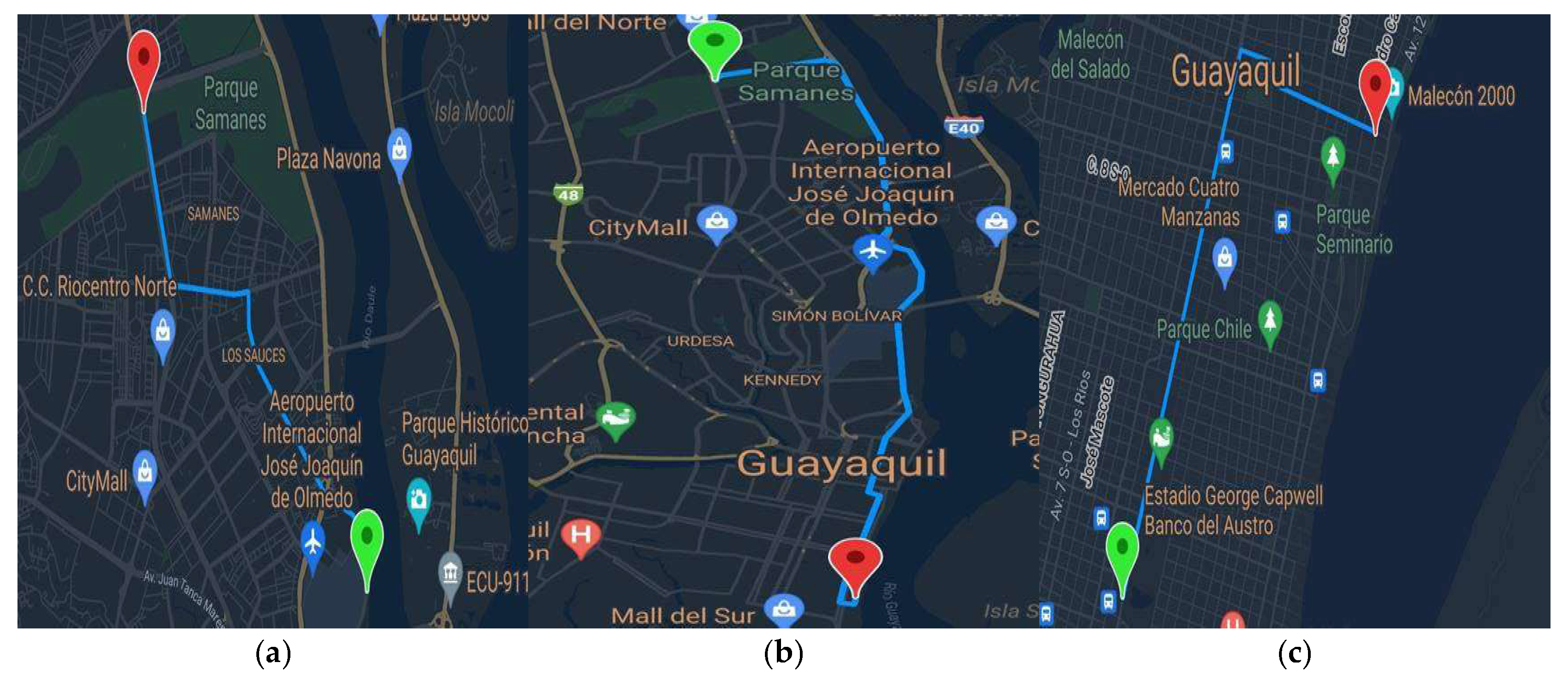
Route 1, represented in
Figure 1 (a), has an extension of 7.9 kilometers, the route started on Benjamin Rosales Avenue, near the Logistics and Global Shipping Service (UPS), and ended at the main entrance of Samanes Park on Francisco de Orellana Avenue, an area known for its high congestion during the morning hours, starting at 7:00 am. Route 2, shown in
Figure 1 (b), has a length of 17.7 kilometers. The route started at the main entrance of Samanes Park, passing through Paseo del Parque Avenue and Narcisa de Jesus Highway, and ended at the Salesian Polytechnic University. On the other hand, Route 3, shown in
Figure 1 (c), is 3.7 kilometers long and started on Quito Avenue at Ayacucho, and ended on 9 de Octubre Avenue, near the Civil Registry Office (Guayaquil Main Office, Rocafuerte), selected for the heavy traffic it experiences in the mornings, specifically from 8:00 am onwards.
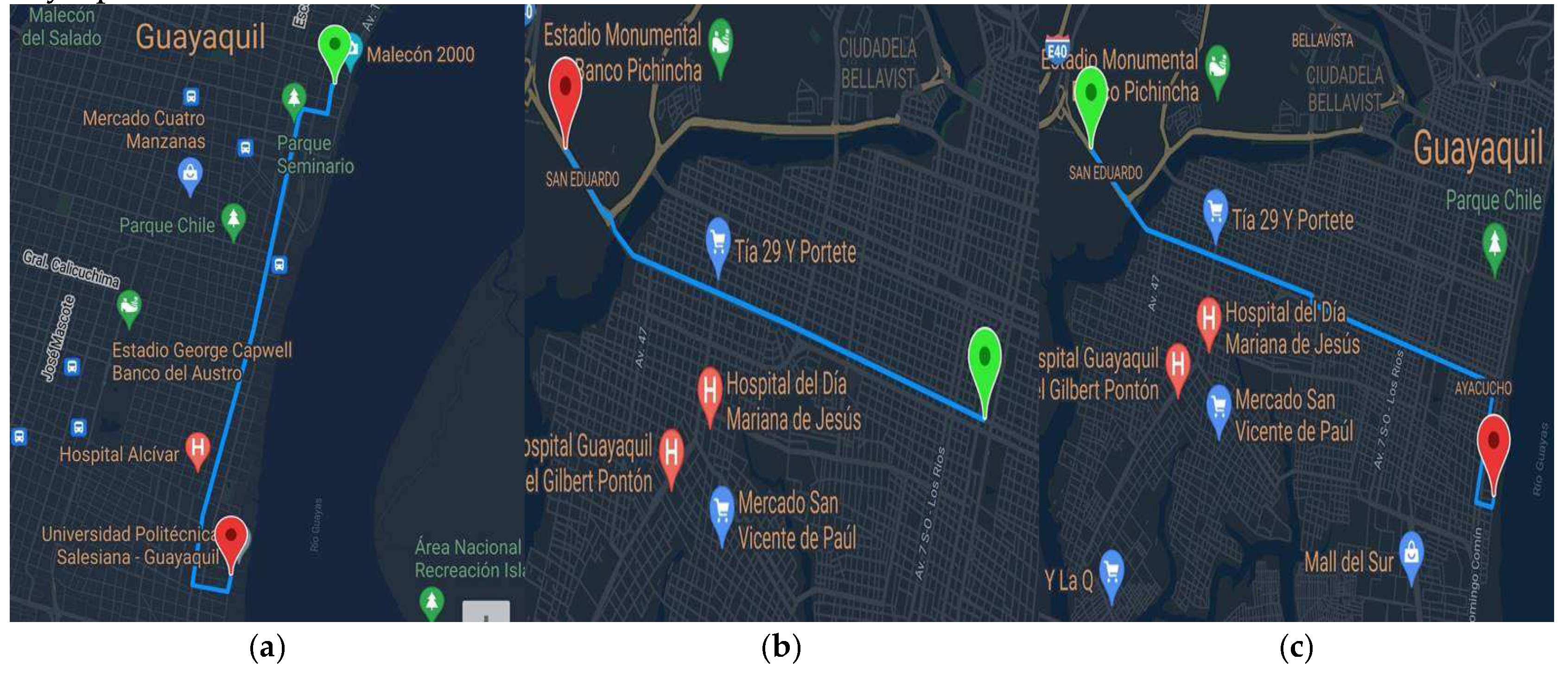
Route 4, shown in
Figure 2 (a), has a distance of 4 kilometers, it started at the Civil Registry (Guayaquil Main Office, Rocafuerte) and ended at the Salesian Polytechnic University, covering a specific route within the city. Route 5, shown in
Figure 2 (b), has an extension of 3.3 kilometers, started on Portete Avenue at 17th Street and ended at Rodriguez Bonin Avenue, particularly at Bazzuka Bodega, an area known for its high morning traffic after 7:00 am. Finally, Route 6, represented in
Figure 2 (c), has a route of 8.6 kilometers, it started from Rodríguez Bonin Avenue, specifically Bazzuca Bodega, to the Universidad Politécnica Salesiana Campus Centenario, thus completing the set of routes established for the study in different areas and times of significant traffic within Guayaquil.
2.1.2. Vehicle Selection and Sampling
A Toyota Corolla model year 2022 hybrid vehicle was analyzed, with specifications as shown in
Table 1.
For data acquisition, the vehicle was driven in Normal, Eco and Power modes.
The normal mode is activated by default and offers a balance between performance and fuel economy, using the thermal or electric motor according to the driver’s needs; it is usually used in city and highway driving. On the other hand, the Eco mode prioritizes the use of the electric motor limiting the thermal engine, so the acceleration response is reduced, as well as the air conditioning system working gradually prioritizing energy saving, the combustion engine is activated only, when necessary, it is usually used in short trips. Finally, the Power mode uses both the electric motor and the combustion engine working together delivering the most power and torque when driving, which allows a more effective and efficient driving, it is ideal for overtaking or fast driving [
21].
2.1.3. Measurement and Data Collection Instruments
An “OBDLINK MX” diagnostic device was used as a tool for fuel consumption data acquisition. This device is compatible with the different versions of OBDII that can operate wirelessly via Bluetooth technology or connect to the OBDII diagnostic port under the vehicle’s dashboard. It provides information on engine performance, emissions, fault codes, etc.
It should be emphasized that the use of OBD LINK MX+ in performing fuel consumption tests is supported by ISO 15765-4:2016, issued by the International Organization for Standardization (ISO). This standard establishes the requirements for in-vehicle diagnostic communication via the controller area network (CAN). By using OBD LINK MX+, compliance with this standard is ensured, enabling accurate data collection, and by being supported by internationally recognized standards, it ensures the validity and reliability of the results obtained during consumer testing [
22].
For its operation this device used the “OBDWiz” software, a Windows application, which, through an intuitive interface and solid architecture, allows communication with the ECU (engine control unit) of the car, enabling real-time extraction of data and analysis of key parameters of the vehicle’s performance and good condition, expanding its versatility in vehicle diagnostics. The GPS Speedometer application was also used, which has speed tracking, navigation maps and distance tracker functions, combining a speedometer with a digital odometer and a classic odometer to measure the distance traveled on a trip. The application offers speed warning alarm, and details such as altitude, longitude, GPS location, and number of connected satellites.
Key features of the application include accurate speed measurement, display of detailed information, display in different units, classic and digital HUD (Head-Up Display) modes, GPS navigation functions, both online and offline modes, and finally mobile battery percentage indication.[
23] On the other hand, the application was used to measure the speed of the vehicle and the speed of the vehicle. On the other hand, Google Maps was also used, an application with more than one billion monthly users, which stands out as the most popular option globally for cartographic navigation. Its all-encompassing presence, available in most countries, including developing countries in Southeast Asia, extends its global reach significantly.
Google Maps as such offers specific features designed to facilitate location identification through search, navigation and traffic management functions for efficient route selection. The ability to build and share routes through the Google My Maps interface adds versatility. In addition, the Google Maps platform includes cloud-based databases (APIs) that store information on travel times and distances of road segments, being usable in the delivery management system (DSM).[
24]
2.1.4. Data Collection Methodology
To start the data collection process, the specifications for evaluating fuel consumption according to the SAE J1321 standard, developed by the Society of Automotive Engineers (SAE), were considered. This standard ensures that the values obtained meet the standardized requirements to be valid. According to Flores [
25], some key aspects of the SAE J1321 standard include a Test Cycle, which represents a specific driving cycle that simulates typical on-road operating conditions for commercial vehicles, covering accelerations, decelerations and load conditions.
The standard establishes requirements for Instrumentation, which details the standards for test equipment, including the accurate measurement of fuel level, vehicle speed and distance traveled. In addition, the Test Procedures describe the specific steps to be followed during testing, such as instrument calibration, data collection and the method for calculating fuel consumption. Finally, the Results report defines the presentation of the test results, including information on test conditions, fuel consumption values and any corrections applied.
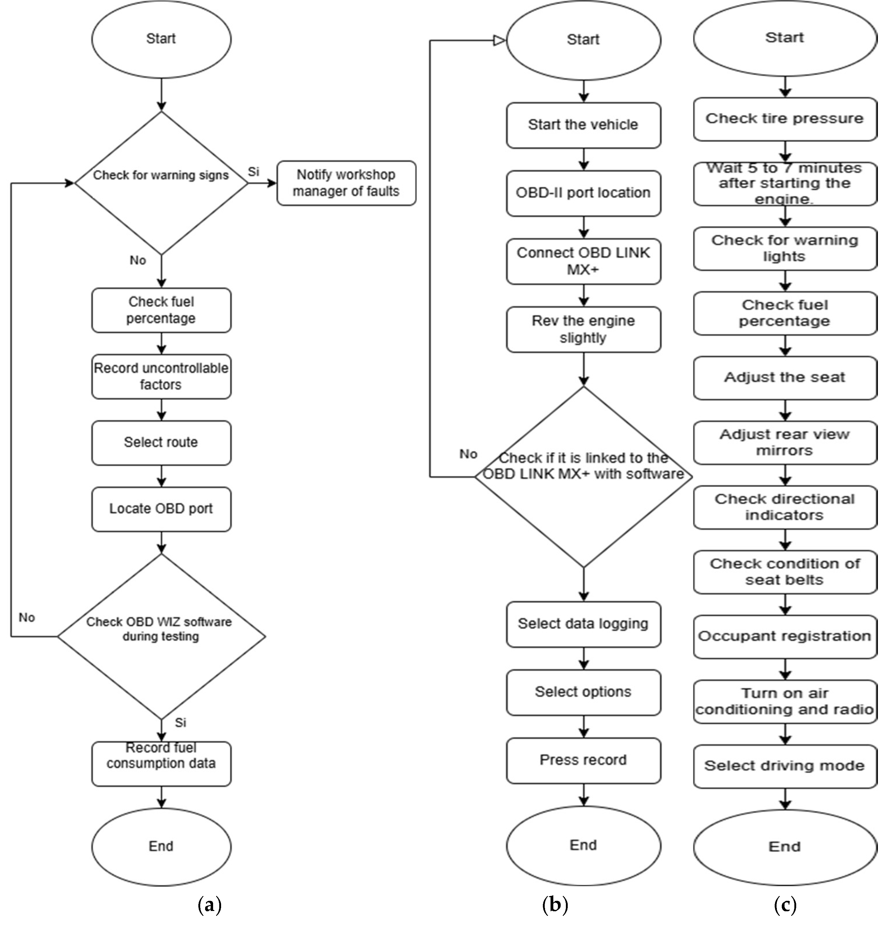
A flow chart explaining in detail the process used to acquire data is shown in
Figure 3 (a) below: first, the vehicle was started and checked for the presence of any warning indicators on the dashboard. If any anomaly was detected, the person in charge of the corresponding Automotive Engineering workshop was informed. In the absence of warnings, the fuel level was checked. In addition, uncontrollable factors, such as ambient temperature, relative humidity and road conditions, among others, were recorded.
Then, the route is chosen, and in turn the vehicle’s OBD port is located and the OBD LINK MX+ acquisition tool is connected. Finally, you run the OBD WIZ software on an electronic device (such as a laptop computer), which will archive the fuel consumption data for further analysis. For the acquisition of data in real time with the help of OBD LINK MX+ it is essential to follow a procedure in each route established as shown in
Figure 3 literal (b), then, a series of steps to be followed in each route was performed [
26].
Start the vehicle.
Locate the OBD-II Port.
Connect the OBD LINK MX+ to the vehicle’s OBD-II port.
Accelerate the vehicle so that the OBD-II can receive real-time data.
Verify if the OBD LINK MX+ digital tool is linked to the OBDWIZ software.
Select the data logging option.
Choose the options that you need to know in this case were (Vehicle speed (km/h), Engine RPM, Fuel Rate (gal/hr).
Select the option record to take the data in real time.
To carry out the study, a driving protocol was performed as shown in
Figure 3 (c), it should be noted that this process was applied at the beginning of each day of testing. The following is the series of steps:
Verify the tire pressure (32 psi in front and rear tires).
Wait 5 to 7 minutes after starting the vehicle for the combustion engine to warm up and in turn charge the batteries.
Check if there are warning lights on the vehicle.
Check the fuel percentage.
Adjust the seat for the driver’s comfort while driving.
Adjust the rear-view mirrors according to the driver to allow him to observe his surroundings.
Check if the directional flashers are in proper working order.
Inspect the condition of the seat belts.
Record the number of occupants (2 occupants for the study).
Turn on air conditioning and radio. (Considered for the study).
Select the driving mode to get to the starting point of our study.
2.2. Data Analysis Tools
Minitab software, which is a statistical analysis application, was used as a tool for research and data analysis in various fields, providing a platform that allows users to re-perform exploratory data analysis, hypothesis testing, statistical modeling, and quality control with scientific accuracy. Its intuitive user interface and numerous statistical functions make it easy to conduct research and make informed data-driven decisions in both academic and industry settings [
27]. Notable within this statistical analysis are measures of central tendency to understand the distribution of data, including the mean for the arithmetic average of fuel consumption values for a numerical representation of the trend of results, and dispersion to find outliers [
28].
2.3. Data Analysis Methodology
Three types of variables were collected and analyzed, which can be divided into countable, non-countable and response variables and are detailed in
Table 2.
3. Results
From the fuel consumption rate obtained by the OBD LINK MX+, this is converted from the unit gallons per hour (Gal/Hr) to gallons per kilometer (Gal/Km) since this is the objective of this study, for this was done as follows:
3.1. Pilot Test
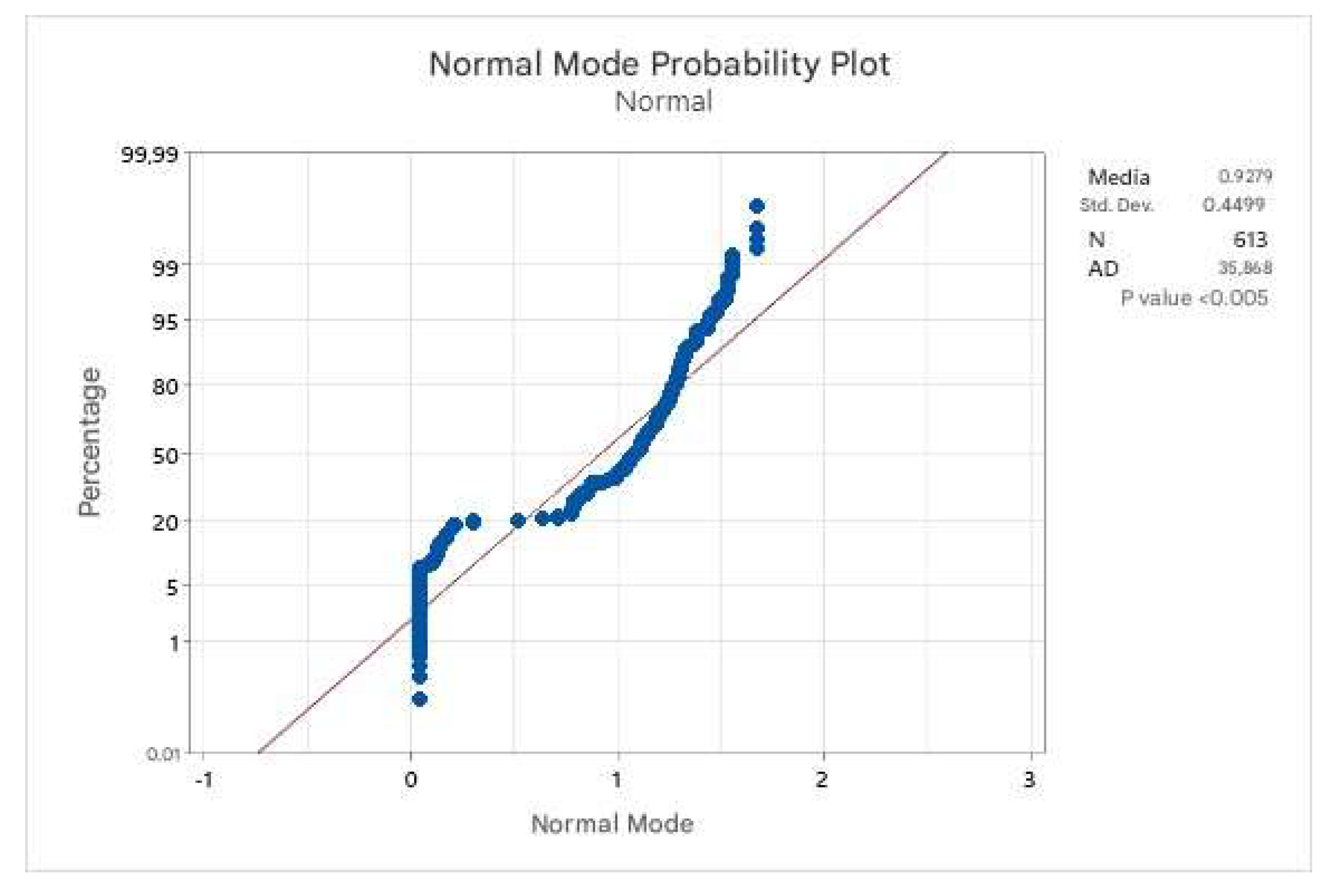
A pilot test was performed on all the routes established as shown in
Table 3, in the different driving modes to determine the number of replicates of the experiment, and thus be able to process the data in the Minitab software, followed by a normality test on the 613 data obtained from a route, in order to verify if they follow the normal distribution as shown in
Appendix B1. The normality test performed is the Anderson-Darling test, which shows that the data does not follow the normal distribution, so the median was taken as a representative value for the set of data acquired during the pilot test, in order to determine the fuel consumption rate of each route in its respective mode of conduction.
With the consumption rate of the 18 treatments of the pilot test we obtained the standard deviation (0.002679) and the standard error (0.000632) to be able to estimate the sample size, this was processed in the Minitab software giving a value of 72 observations, which in turn we divided it for the 18 treatments that were carried out in one run, which implies that 4 replicates should be carried out in the experiment. As shown in
Table 4.
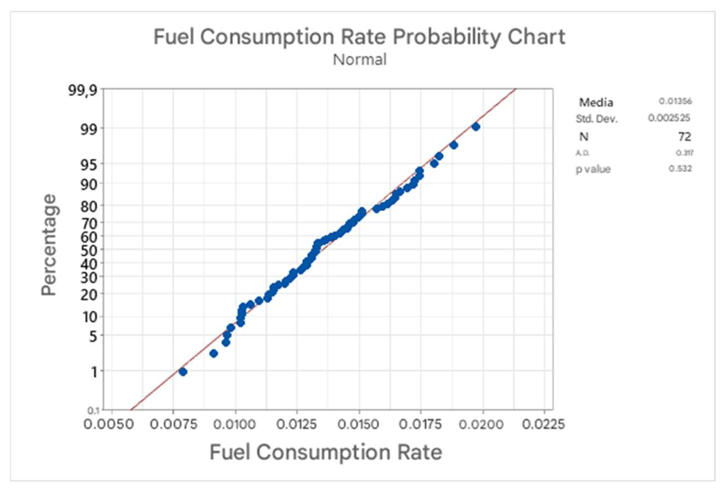
3.2. Normality Test
Once the 4 replicates of the experiment were carried out, we proceeded with the statistical analysis of this study, where it is necessary to examine the distribution of the data collected [
29].
Figure 4 shows the Anderson-Darling normality test, which was performed on the 72 fuel consumption rate data obtained in the experiment, where this test shows that these data follow the normal distribution.
Since the fuel consumption rate data of the experiment follows the normal distribution, the arithmetic mean was used to estimate the pro-average consumption rate of each route, in the respective driving modes as shown in Table (5), (6), (7).
3.3. Routes
3.3.1. Results Normal Mode Routes
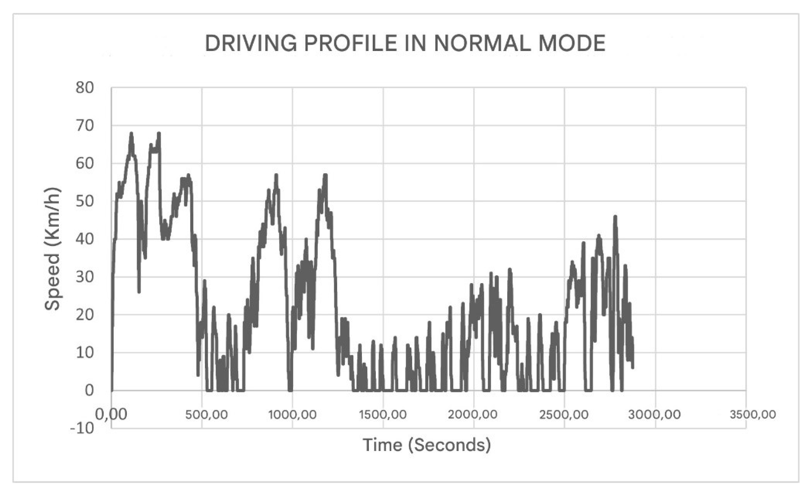
The results obtained during the tests in Normal driving mode during the 6 routes are shown in
Table 5. In addition,
Figure A2 in
Appendix B shows the driving profile: total speed of the route versus total time, taking route 2 of the experiment with its respective speed and time data from repetition 2 of 4, since this has the longest distance traveled.
3.2.2. Results Eco Mode Routes
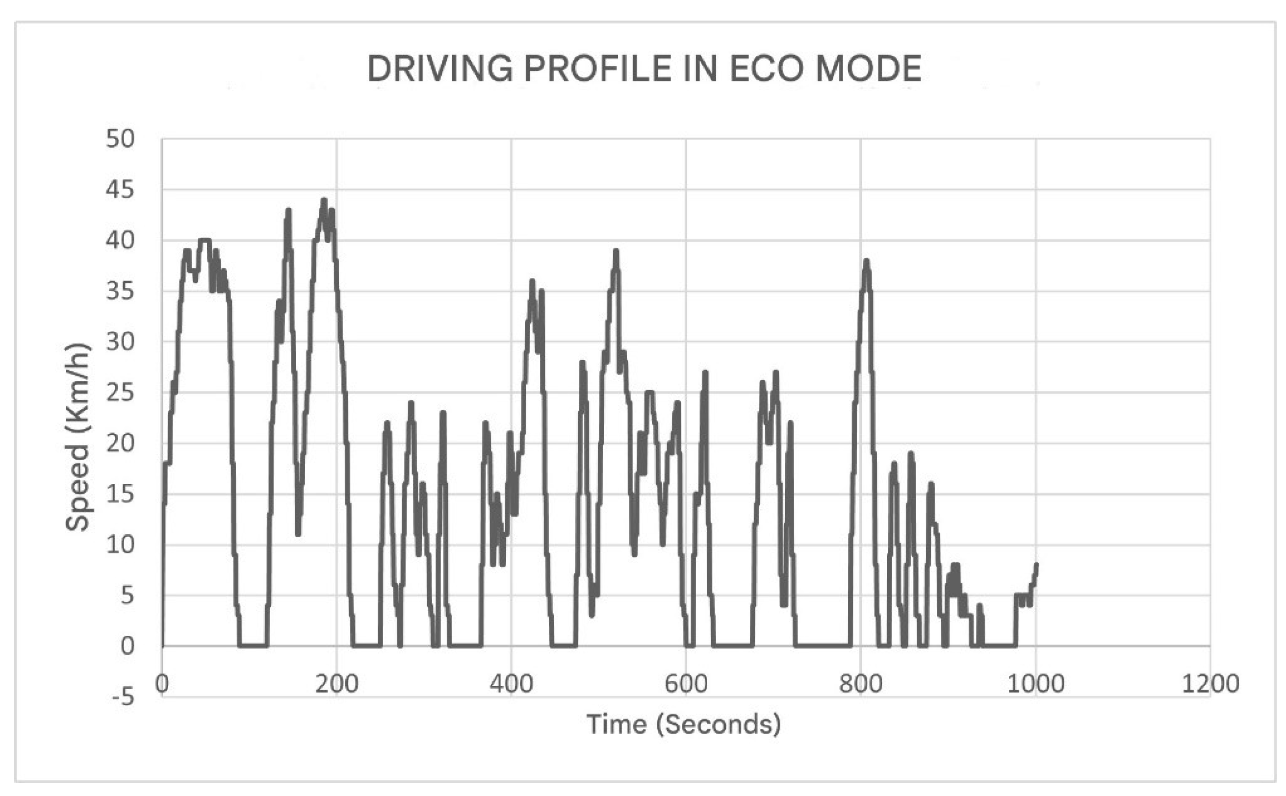
The results obtained during the tests in Eco driving mode during the 6 routes are shown in
Table 6. In addition,
Figure A3 in
Appendix B shows the driving profile: total travel speed versus total time, taking route 2 of the experiment with its respective speed and time data from repetition 2 of 4, since this has the longest travel distance.
3.3.3. Results Power Mode Routes
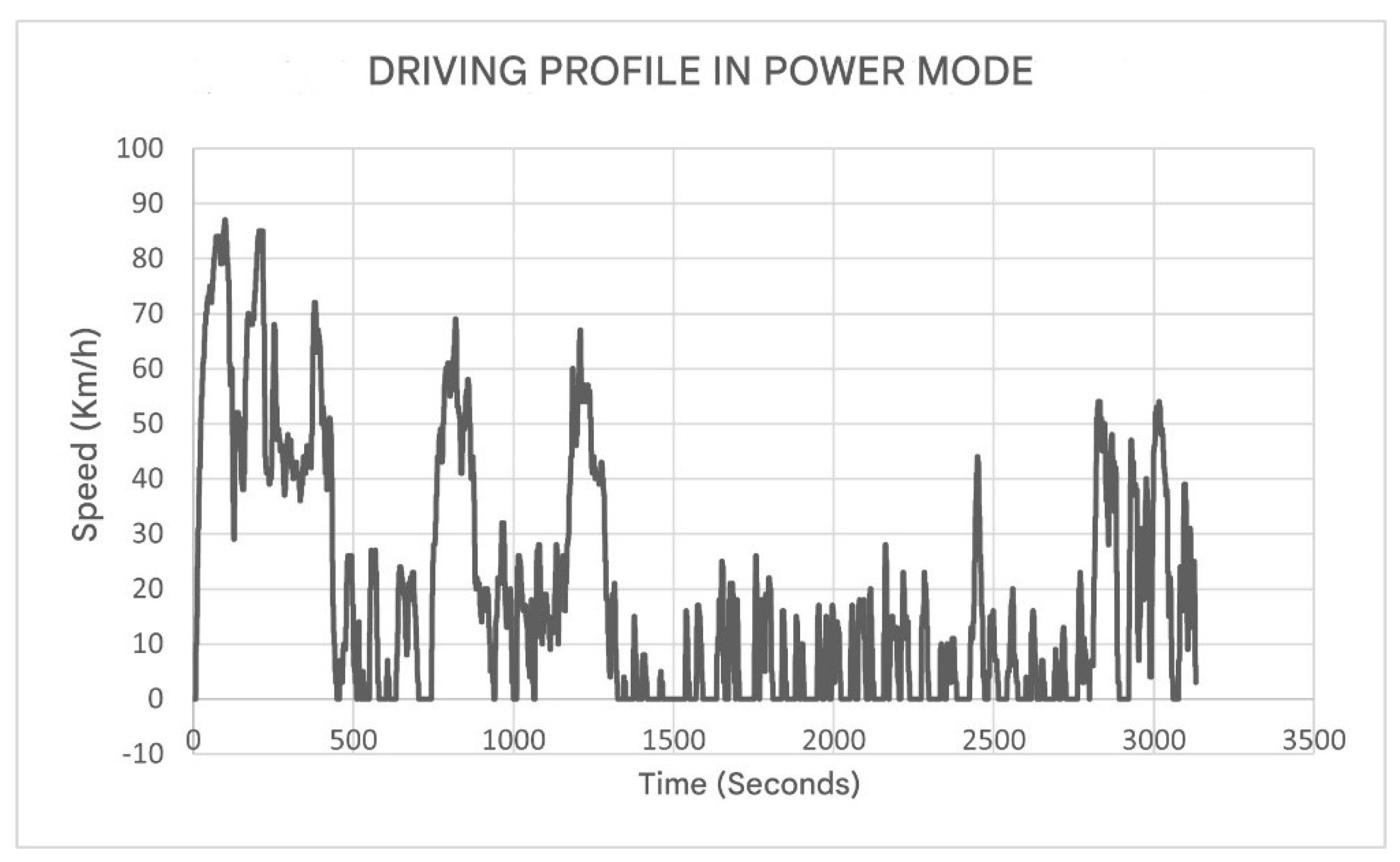
The results obtained during the tests in Power Driving Mode in the 6 routes are shown in
Table 7. In addition,
Figure A4 in
Appendix B shows the driving profile: total speed of the trip versus total time, taking route 2 of the experiment and its respective speed and time data of repeats 3 of 4, because this has the longest distance of travel.
3.4. Correlation Analysis
Table 8 shows the average values in the different driving modes such as: maximum speed, average speed, distance, time and fuel consumption rate per kilometer traveled.
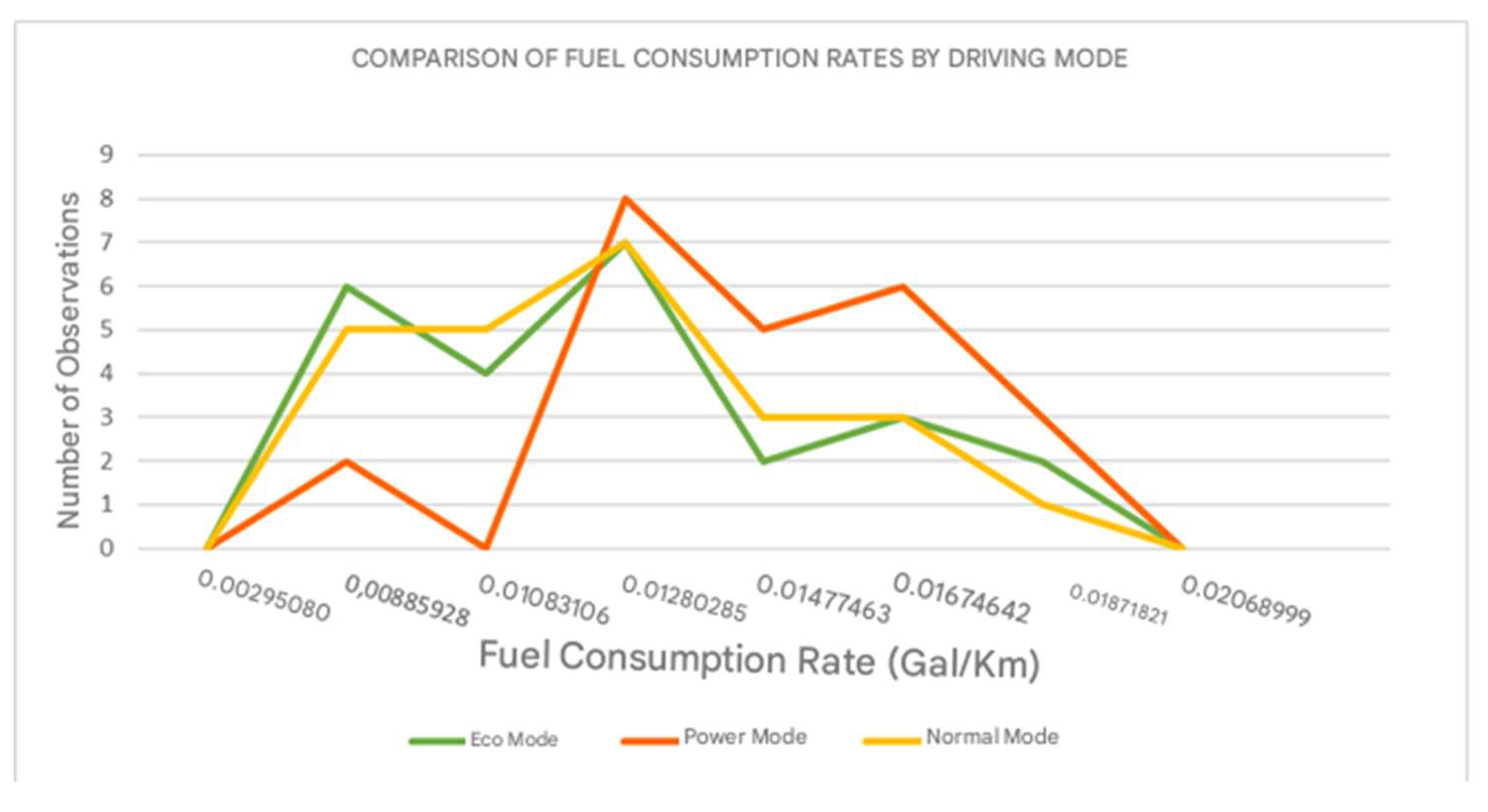
Next, the frequency polygon graph is observed in
Figure 5, where it shows the comparison of the fuel consumption rates per kilometer traveled, of the three driving modes as they are (Normal, Eco, Power), this graph is constructed from the Frequency
Table A4,
Table A5,
Table A6 in
Appendix A section.
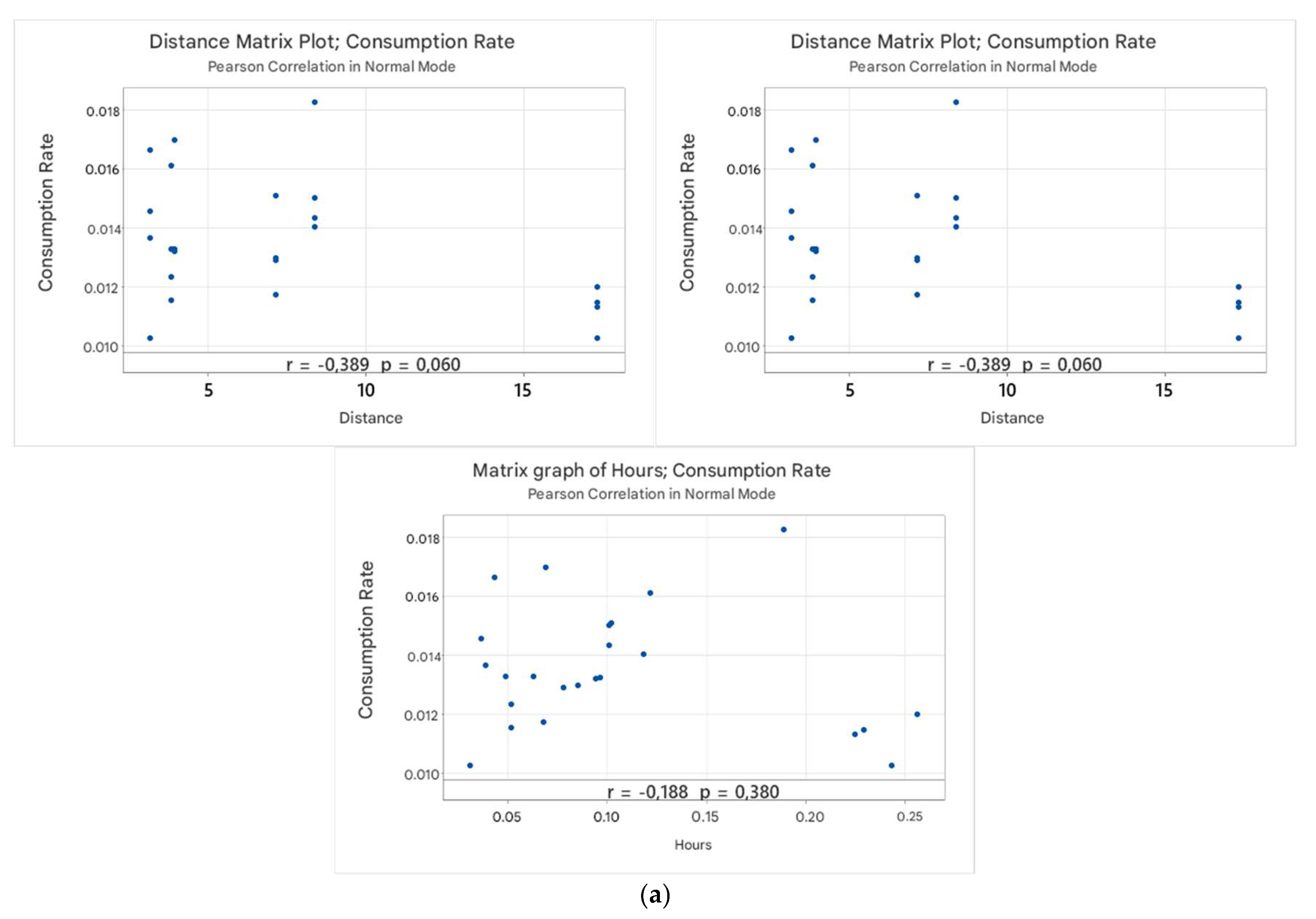
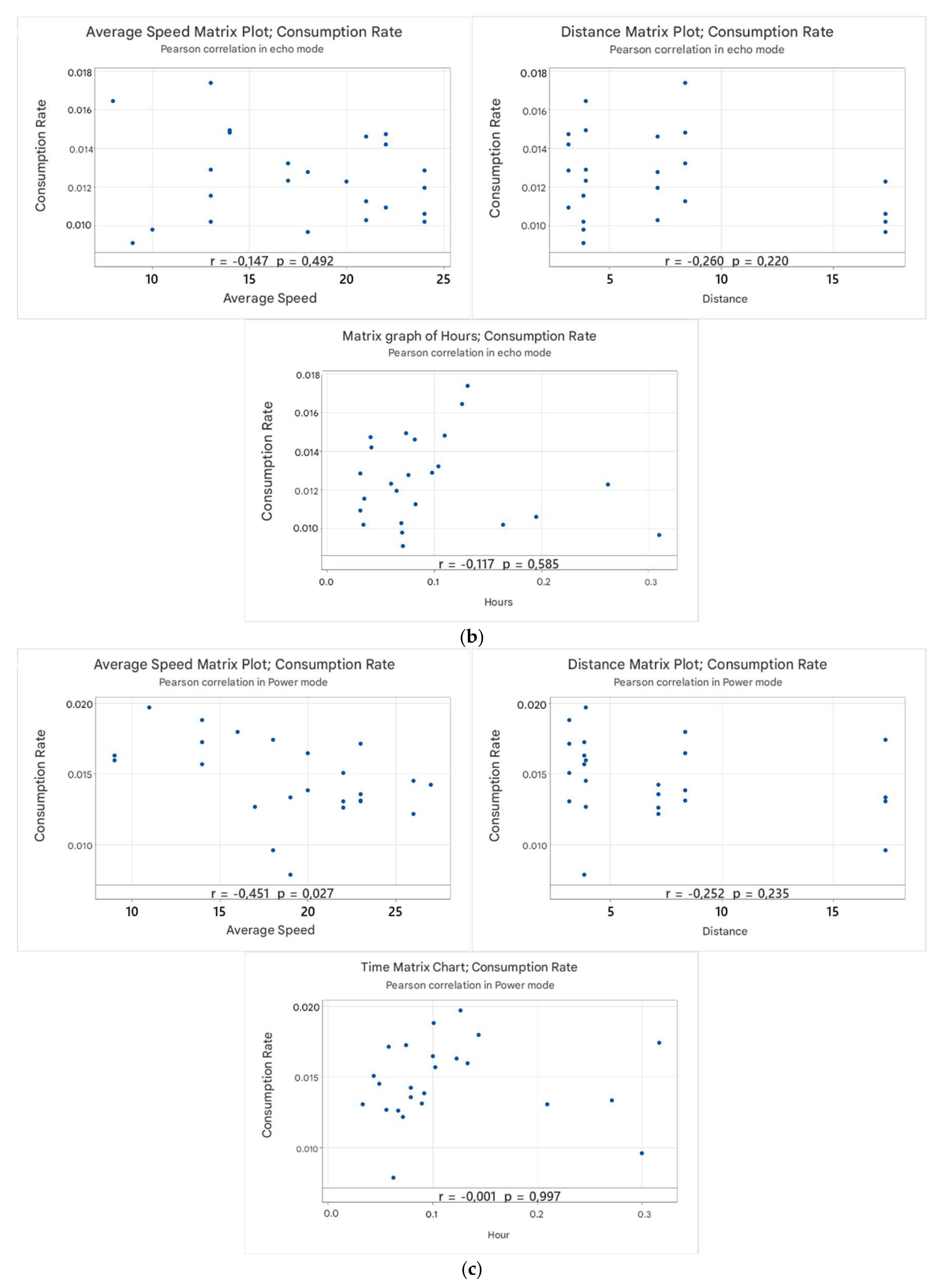
The values of Pearson’s correlation coefficient R and the determination coefficient R^2 were obtained as shown in
Table 9. On the other hand,
Figure 6 (a), (b), (c), shows the correlation graphs of the three modes Normal, Eco and Power. Given the results of the correlation analysis of the factors studied with respect to the consumption rate, we have: In the average speed variable in the 3 modes the relationship is inverse where in the Eco mode there is a very low correlation, in the Normal mode there is a low correlation and in the Power mode there is a moderate correlation. In the travel time variable in the 3 modes the relationship is inverse where in the Eco and Normal modes have a very low correlation and in the Power mode it has a null correlation. In the distance variable in the 3 modes the relationship is inverse where in Eco, Normal and Power modes have a low correlation.
3.5. Costs
3.5.1. Cost Result Normal, Eco and Power Mode
The results of the average costs, gallons per fuel consumption in dollars obtained during the tests in Normal, Eco and Power driving modes for the 6 routes are shown in
Table 10.
For the cost study, the Normal mode was taken as the main base, where a value of $8.45 US dollars was obtained, with respect to the Eco mode a difference of $0.71 US cents was analyzed, which meant a saving of 8.4% in fuel, likewise with respect to the Power mode there is an increase of $0.47 US cents, which meant an increase in fuel consumption of 5.56%. It should be noted that 92 octane super gasoline was used for the test, with a market value per gallon of $3.61 in the month of December 2023.
4. Discussion
The present study is of practical interest, analyzing how the fuel consumption rate is influenced by the factors studied such as: distance traveled, time and average speed, as well as traffic conditions and the usual behavior of a driver in a large city as in the study by Shirk and Geller [
9], and with this to determine the fuel consumption rate per kilometer traveled in urban routes in the city of Guayaquil.
The experiment was conducted on different routes with a total distance of 175.2 km, where the condition of the roads for the routes in the North and Central part are in good condition, on the other hand, the routes in the West zone the condition of the roads are mostly irregular, due to the fact that they are under maintenance. At the same time, this experimental study is carried out in the month of December, with high traffic during peak hours, due to the Christmas and New Year’s holidays.
According to the vehicle’s technical data sheet on fuel consumption efficiency in urban trips, it is 1.03 gallons per 100 kilometers [
21], based on controlled conditions and which does not indicate the driving mode in which this test is carried out. As our study was based on real conditions, we have as a result that, for every 100 kilometers in Normal mode 1.33 gallons were consumed, in Eco mode 1.22 gallons and in Power mode 1.41 gallons, and these are close compared to what the manufacturer claims.
The results obtained could be used for future studies with internal combustion engine (ICE) and hybrid vehicles (HEV) [
11], making use of the digital tool OBD LINK MX+ [
30], for data collection due to its wide variety of functions and uses can be an important part to determine the rate of fuel consumption per kilometer traveled and compare with an internal combustion engine (ICE) vehicle.
5. Conclusions
The study identified fuel consumption behaviors in different urban scenarios and driving modes (Normal, Eco, Power), where information was provided on how the factors: average speed, traffic conditions, usual driving style in urban driving and time affect the fuel consumption efficiency of the study vehicle. Based on Pearson’s correlation analysis and the coefficient of determination, the most influential factors in the study were identified as: average speed with a higher percentage of influence in Normal and Power modes, compared to Eco mode. The time factor was determined to have no significant influence on any driving mode. In the distance factor, there was a considerable percentage of influence only in Normal mode, compared to the other two modes.
For the acquisition of data in real time, the OBD LINK MX+ digital tool was used, having an approximate average of 500 to 5000 data for each route, depending on the distance and time traveled. In addition, the OBDWIZ software was used to visualize the data during urban routes established in routes (North, Center and West), within the city of Guayaquil. With the help of Minitab software, procedures such as: normality test and a cor-relation analysis of the data obtained in each driving mode, in the Toyota Corolla Hybrid 2022 during urban journeys in the city of Guayaquil, which revealed a fuel consumption rate per kilometer traveled of 0.013536 Gal/km in Normal driving mode, 0.012472 Gal/km in Eco mode and 0.014658 Gal/km in Power mode, it was highlighted that the Eco mode in the conditions for this experiment there was an optimization in fuel saving efficiency, unlike the Power mode that its consumption rate was higher compared to the other two modes.
During the data acquisition of this study, in the Eco mode, a fuel saving of 8.4% could be observed with respect to Normal mode, since there was more work of the electric motor, so the response of the accelerator pedal is reduced, as well as the air conditioning system working gradually, the combustion engine is activated only when necessary. In Power mode, there was an increase in fuel consumption of 5.56% with respect to Normal mode, due to the fact that this mode works with the electric motor and the internal combustion engine, which allows more efficient driving, due to the increased sensitivity of the accelerator pedal.
Appendix A
Table A1.
Normal Mode Costs.
Table A1.
Normal Mode Costs.
| Normal driving mode |
|---|
| Routes |
Gallons Consumed |
Travel time (Hours) |
Cost |
Total Cost |
| 1 |
0,080097770 |
0,085138333 |
$0,33 |
$1,33 |
| 1 |
0,109202524 |
0,102360000 |
$0,39 |
| 1 |
0,074173586 |
0,067776667 |
$0,27 |
| 1 |
0,095083310 |
0,078055000 |
$0,34 |
| 2 |
0,198317442 |
0,256526667 |
$0,72 |
$2,92 |
| 2 |
0,187153410 |
0,229166667 |
$0,68 |
| 2 |
0,217253869 |
0,243333333 |
$0,78 |
| 2 |
0,203888470 |
0,224860000 |
$0,74 |
| 3 |
0,078789600 |
0,121943333 |
$0,28 |
$0,82 |
| 3 |
0,042255924 |
0,051388333 |
$0,15 |
| 3 |
0,049732896 |
0,051666667 |
$0,18 |
| 3 |
0,059999826 |
0,062776667 |
$0,21 |
| 4 |
0,063083442 |
0,094166667 |
$0,23 |
$0,91 |
| 4 |
0,071260500 |
0,096666667 |
$0,26 |
| 4 |
0,052075563 |
0,048888333 |
$0,18 |
| 4 |
0,066750400 |
0,069166667 |
$0,24 |
| 5 |
0,028964240 |
0,030693333 |
$0,11 |
$0,61 |
| 5 |
0,037533674 |
0,036666667 |
$0,14 |
| 5 |
0,043004720 |
0,038471667 |
$0,16 |
| 5 |
0,056395750 |
0,043333333 |
$0,20 |
| |
6 |
0,100509250 |
0,118193333 |
$0,36 |
$1,86 |
| |
6 |
0,102542230 |
0,101110000 |
$0,38 |
| |
6 |
0,121588987 |
0,101110000 |
$0,44 |
| |
6 |
0,189425172 |
0,189026667 |
$0,68 |
Table A2.
Eco Mode Costs.
Table A2.
Eco Mode Costs.
| Eco driving mode |
|---|
| Routes |
Gallons Consumed |
Travel time (Hours) |
Cost |
Total Cost |
| 1 |
0,083298610 |
0,075833333 |
$0,30 |
$1,24 |
| 1 |
0,070940200 |
0,069026667 |
$0,26 |
| 1 |
0,085048944 |
0,064443333 |
$0,31 |
| 1 |
0,102878523 |
0,081526667 |
$0,37 |
| 2 |
0,170856978 |
0,195138333 |
$0,61 |
$2,86 |
| 2 |
0,161297130 |
0,164321667 |
$0,58 |
| 2 |
0,229780143 |
0,262083333 |
$0,83 |
| 2 |
0,233863864 |
0,309860000 |
$0,84 |
| 3 |
0,049964200 |
0,070276667 |
$0,18 |
$0,68 |
| 3 |
0,034285300 |
0,033888333 |
$0,12 |
| 3 |
0,046561240 |
0,034716667 |
$0,17 |
| 3 |
0,058375500 |
0,070555000 |
$0,21 |
| 4 |
0,011283909 |
0,073471667 |
$0,04 |
$0,81 |
| 4 |
0,067418194 |
0,097916667 |
$0,24 |
| 4 |
0,055577640 |
0,059583333 |
$0,20 |
| 4 |
0,093129630 |
0,125555000 |
$0,33 |
| 5 |
0,030313990 |
0,030693333 |
$0,11 |
$0,55 |
| 5 |
0,034685269 |
0,040693333 |
$0,13 |
| 5 |
0,042240319 |
0,030833333 |
$0,15 |
| 5 |
0,045160987 |
0,040971667 |
$0,16 |
| 6 |
0,103563716 |
0,103750000 |
$0,37 |
$1,60 |
| 6 |
0,121690070 |
0,130971667 |
$0,44 |
| 6 |
0,126036971 |
0,109583333 |
$0,45 |
| 6 |
0,095751094 |
0,082083333 |
$0,34 |
Table A3.
Power Mode Costs.
Table A3.
Power Mode Costs.
| Power driving mode |
|---|
| Routes |
Gallons Consumed |
Travel time (Hours) |
Cost |
Total Cost |
| 1 |
0,076829841 |
0,07180556 |
$0,28 |
$1,30 |
| 1 |
0,085230728 |
0,07944440 |
$0,31 |
| 1 |
0,094704360 |
0,06736111 |
$0,34 |
| 1 |
0,104079600 |
0,07902778 |
$0,37 |
| 2 |
0,228325226 |
0,31652778 |
$0,82 |
$3,29 |
| 2 |
0,187075620 |
0,20930556 |
$0,68 |
| 2 |
0,256792800 |
0,27125000 |
$0,92 |
| 2 |
0,240141330 |
0,30000000 |
$0,87 |
| 3 |
0,062534518 |
0,10250000 |
$0,23 |
$0,98 |
| 3 |
0,079659450 |
0,12319444 |
$0,29 |
| 3 |
0,072284795 |
0,07444440 |
$0,26 |
| 3 |
0,056289357 |
0,06277780 |
$0,20 |
| 4 |
0,046914312 |
0,05611110 |
$0,17 |
$0,98 |
| 4 |
0,083269837 |
0,13347222 |
$0,30 |
| 4 |
0,091525106 |
0,12694400 |
$0,33 |
| 4 |
0,051801191 |
0,04916670 |
$0,18 |
| 5 |
0,064808790 |
0,10083300 |
$0,24 |
$0,70 |
| 5 |
0,036556290 |
0,03366667 |
$0,13 |
| 5 |
0,052116690 |
0,05383333 |
$0,18 |
| 5 |
0,041822470 |
0,04402778 |
$0,15 |
| |
6 |
0,126922750 |
0,14375000 |
$0,46 |
$1,67 |
| |
6 |
0,109261710 |
0,10055600 |
$0,39 |
| |
6 |
0,109655680 |
0,09000000 |
$0,39 |
| |
6 |
0,120432420 |
0,09194333 |
$0,43 |
Table A4.
Data grouping using the frequency polygon Echo mode.
Table A4.
Data grouping using the frequency polygon Echo mode.
| |
|
FREQUENCIES |
|
| CATEGORIES |
ABSOLUTE |
RELATIVE |
CLASS MARK |
| 0 |
0,00772023 |
0 |
0% |
0,00386012 |
| 0,00910600 |
0,01049178 |
6 |
25% |
0,00979889 |
| 0,01049178 |
0,01187755 |
4 |
17% |
0,01118466 |
| 0,01187755 |
0,01326332 |
7 |
29% |
0,01257044 |
| 0,01326332 |
0,01464909 |
2 |
8% |
0,01395621 |
| 0,01464909 |
0,01603487 |
3 |
13% |
0,01534198 |
| 0,01603487 |
0,01742064 |
2 |
8% |
0,01672775 |
| 0,01742064 |
0,01880641 |
0 |
0% |
0,01811353 |
| Total |
24 |
100% |
|
Table A5.
Clustering of data using the frequency polygon Normal mode.
Table A5.
Clustering of data using the frequency polygon Normal mode.
| |
|
FREQUENCIES |
|
| CATEGORIES |
ABSOLUTE |
RELATIVE |
CLASS MARK |
| 0 |
0,008846950 |
0 |
0% |
0,004423475 |
| 0,01027584 |
0,011704734 |
5 |
21% |
0,010990287 |
| 0,01170473 |
0,013133629 |
5 |
21% |
0,012419181 |
| 0,01313363 |
0,014562523 |
7 |
29% |
0,013848076 |
| 0,01456252 |
0,015991418 |
3 |
13% |
0,015276971 |
| 0,01599142 |
0,017420313 |
3 |
13% |
0,016705865 |
| 0,01742031 |
0,018849207 |
1 |
4% |
0,018134760 |
| 0,01742031 |
0,018849207 |
0 |
0% |
0,018134760 |
| Total |
24 |
100% |
|
Table A6.
Clustering of data using the frequency polygon Power mode.
Table A6.
Clustering of data using the frequency polygon Power mode.
| |
|
FREQUENCIES |
|
| CATEGORIES |
ABSOLUTE |
RELATIVE |
CLASS MARK |
| 0 |
0,00590159 |
0 |
0% |
0,00295080 |
| 0,00787338 |
0,00984517 |
2 |
8% |
0,00885928 |
| 0,00984517 |
0,01181695 |
0 |
0% |
0,01083106 |
| 0,01181695 |
0,01378874 |
8 |
33% |
0,01280285 |
| 0,01378874 |
0,01576053 |
5 |
21% |
0,01477463 |
| 0,01576053 |
0,01773231 |
6 |
25% |
0,01674642 |
| 0,01773231 |
0,0197041 |
3 |
13% |
0,01871821 |
| 0,0197041 |
0,02167589 |
0 |
0% |
0,02068999 |
| Total |
24 |
100% |
|
Appendix B
Figure A1.
Normality test of path 1 Normal mode.
Figure A1.
Normality test of path 1 Normal mode.
Figure A2.
Driving cycle Normal mode route 2 repetition 2 of 4.
Figure A2.
Driving cycle Normal mode route 2 repetition 2 of 4.
Figure A3.
Driving cycle Eco route mode 2 repetition 2 of 4.
Figure A3.
Driving cycle Eco route mode 2 repetition 2 of 4.
Figure A4.
Power route mode driving cycle 2 repeat 3 of 4.
Figure A4.
Power route mode driving cycle 2 repeat 3 of 4.
References
- O. Abigail, “CO2: emisiones mundiales 1995-2022 | Statista.” Accessed: Dec. 12, 2023. [Online]. Available: https://n9.cl/58d6v.
- C. Ecuador, “Alpina Ecuador reducirá en un 15% sus emisiones de dióxido de carbono.” Accessed: Dec. 14, 2023. [Online]. Available: https://n9.cl/x9b4l.
- A. Jorque, A. Arias, D. Borja y A. Moreno, «Estudio de la utilización del hidrógeno en la industria automotriz: Revisión,» Polo del Conocimiento, vol. 7, nº 10, pp. 1645-1667, 2022.
- INEC, Anuario de Estadísticas de Transporte, 2021, INEC, 2022.
- Q. -Ecuador and P. Edición, “INSTITUTO ECUATORIANO DE NORMALIZACIÓN CONTROL DE EMISIONES CON-TAMINANTES DE FUENTES MÓVILES TERRESTRES,” 2008.
- M. E. Hmidi, I. Ben Salem, and L. El Amraoui, “An efficient method for energy management optimization control: Minimizing fuel consumption for hybrid vehicle applications,” Transactions of the Institute of Measurement and Control, vol. 42, no. 1, pp. 69 – 80, 2020, doi: 10.1177/0142331219874152. [CrossRef]
- F. Pesántez Avilés, L. Álvarez Rodas, and A. Torres Toukoumidis, COVIDA-20 Una coalición educativa para en-frentar la pandemia, 1st ed. Naucalpan de Juaréz: Pearson Educación de México S.A., 2021.
- R. López-Chila, J. Arteaga-Sotomayor, E. Caballero-Barros, and J. Llerena-Izquierdo, “An e-learning evaluation method with the effectiveness of the questionnaire tool in the VLEs,” in 2023 IEEE World Engineering Education Conference (EDUNINE), IEEE, Mar. 2023, pp. 1–6. doi: 10.1109/EDUNINE57531.2023.10102811. [CrossRef]
- R. “ Barney, “ Carlson, M. G. Shirk, B. M. Geller, R. ’ Barney, and ’ Carlson, “Factors Affecting the Fuel Consump-tion of Plug-In Hybrid Electric Vehicles,” EVS25,Shenzhen, China,11/05/2010,11/09/2010, Nov. 2001, Accessed: Dec. 14, 2023. [Online]. Available: https://n9.cl/16k3p.
- J. Rios-Torres, J. Liu, and A. Khattak, “Fuel consumption for various driving styles in conventional and hybrid electric vehicles: Integrating driving cycle predictions with fuel consumption optimization*,” Int J Sustain Transp, vol. 13, no. 2, pp. 123–137, Feb. 2019, doi: 10.1080/15568318.2018.1445321. [CrossRef]
- D. S. Villanueva Huamán, “Evaluación del consumo de combustible y mantenibilidad de un vehículo hibrido So-nata y vehículo convencional Yaris Hatchback,” Repositorio Institucional - UCV, 2020, Accessed: Jan. 31, 2024. [Online]. Available: https://n9.cl/7q6w8.
- Y. Huang et al., “Impact of drivers on real-driving fuel consumption and emissions performance,” Science of The Total Environment, vol. 798, p. 149297, Dec. 2021, doi: 10.1016/J.SCITOTENV.2021.149297. [CrossRef]
- A. V. Shvetsov, “Change in Fuel Consumption of a Hybrid Vehicle When Operating in the Far North,” World Elec-tric Vehicle Journal 2021, Vol. 12, Page 104, vol. 12, no. 3, p. 104, Jul. 2021, doi: 10.3390/WEVJ12030104. [CrossRef]
- Y. Ivanov, R. Ivanov, G. Kadikyanov, G. Staneva, and I. Danilov, “A study of the fuel consumption of hybrid car Toyota Yaris,” Transport Problems, vol. 14, no. 1, pp. 155–167, 2019, doi: 10.21307/TP.2019.14.1.14. [CrossRef]
- R. Granda and R. Gabriel, “Estudio del Consumo de Combustible en Carretera de un Vehículo Híbrido en Modo de Manejo Económico y Deportivo,” 2022, Accessed: Dec. 12, 2023. [Online]. Available: https://n9.cl/jk7ng.
- F. A. Sánchez Flores, “Fundamentos Epistémicos de la Investigación Cualitativa y Cuantitativa: Consensos y Di-sensos,” Revista Digital de Investigación en Docencia Universitaria, pp. 101–122, Apr. 2019, doi: 10.19083/RIDU.2019.644. [CrossRef]
- Primicias, “Guayaquil vuelve a ser la ciudad más poblada de Ecuador.” Accessed: Dec. 14, 2023. [Online]. Availa-ble: https://n9.cl/ajx0e.
- S. Ruata Aviles, F. J. Córdova Rizo, G. Cabeza Quintero, and M. Y. Leyva Vázquez, “Evaluación tráfico vehicular para conocer nivel de servicio de Avenida Francisco de Orellana, Ciudad Guayaquil,” Journal of Science and Re-search: Revista Ciencia e Investigación, vol. 3, pp. 69–73, 2018, Accessed: Jan. 19, 2024. [Online]. Available: https://n9.cl/bt2goh.
- T. Z. Ashhad Verdezoto, F. F. Cabrera Montes, and O. B. Roa Medina, “Análisis del congestionamiento vehicular para el mejoramiento de vía principal en Guayaquil-Ecuador,” Revista Gaceta Técnica, vol. 21, pp. 4–23, 2020.
- El Universo, “Los horarios de mayor tráfico vehicular en Guayaquil y Samborondón,” Guayaquil, May 17, 2022.
- L. E. Hv and X. Hv, “ESPECIFICACIONES TÉCNICAS”.
- International Organization for Standardization, Road vehicles - Diagnostic communication over Controller Area Network (DoCAN) - Part 4: Requirements for emissions-related systems.
- DIGIZONE - Trusted Android Apps- PDF Reader & Documents Tools, “Velocimetro gps - Odometer.” Accessed: Jan. 19, 2024. [Online]. Available: https://n9.cl/kmcyh.
- S. Horng and P. Yenradee, “Delivery Service Management System Using Google Maps for SMEs in Emerging Countries,” Computers, Materials & Continua, vol. 75, no. 3, pp. 6119–6143, 2023, doi: 10.32604/cmc.2023.038764. [CrossRef]
- A. Flores et al., “Prototipo de asistente electrónico para entrenamiento y valoración en estrategias de eco con-ducción para vehículos M1 por OBD II,” Pro Sciences: Revista de Producción, Ciencias e Investigación, vol. 7, no. 47, pp. 58–74, Mar. 2023, doi: 10.29018/ISSN.2588-1000VOL7ISS47.2023PP58-74. [CrossRef]
- “Manual de instrucciones de uso Medidor de diagnóstico automotriz PCE-OBD 2”, Accessed: Dec. 12, 2023. [Online]. Available: www.pce-iberica.eswww.pce-iberica.es.
- E. M. Tocoronte and K. N. G. Z. G. Zuñiga, “Sofware minitab en la predicción del tiempo estándar.,” Sapientia Technological, vol. 2, no. 1, pp. 19–19, Jan. 2021, Accessed: Dec. 12, 2023. [Online]. Available: https://n9.cl/kauwd.
- K. P. Schreiber, G. Braz, C. C. Bertolucci, J. A. Da Silva, and M. Porciúncula, “Levels of understanding for the arithmetic mean concept by adolescents through the piagetian clinical-critical method[Níveis de compreensão do conceito de média aritmética de adolescentes a partir do método clínico-crítico piagetiano],” Bolema - Mathematics Education Bulletin, vol. 33, no. 64, pp. 491–512, Jan. 2019, doi: 10.1590/1980-4415v33n64a03. [CrossRef]
- A. L. F. da Silva, E. L. Noqueira, W. de S. Campos, J. B. de O. Júnior, and M. M. De Albuquerque, “USO DE GRÁ-FICAS DE CONTROL PARA VARIABLES (x Y R): ESTUDIO DEL DIÁMETRO DE LOS TORNILLOS CON EL SOFTWARE MINITAB®[USO DOS GRÁFICOS DE CONTROLE PARA VARIÁVEIS (x E R): ESTUDO SOBRE O DIÂMETRO DOS PA-RAFUSOS UTILIZANDO O SOFTWARE MINITAB®],” Revista de Ingeniería y Tecnología para Aplicaciones Indus-triales Acceso Abierto, vol. 5, no. 18, pp. 105–112, Jun. 2019, doi: 10.5935/2447-0228.20190035. [CrossRef]
- “OBDLink® MX+ Support - The Documents You Need For Your Scan Tool.” Accessed: Feb. 16, 2024. [Online]. Available: https://n9.cl/1mb32n.
|
Disclaimer/Publisher’s Note: The statements, opinions and data contained in all publications are solely those of the individual author(s) and contributor(s) and not of MDPI and/or the editor(s). MDPI and/or the editor(s) disclaim responsibility for any injury to people or property resulting from any ideas, methods, instructions or products referred to in the content. |
© 2025 by the authors. Licensee MDPI, Basel, Switzerland. This article is an open access article distributed under the terms and conditions of the Creative Commons Attribution (CC BY) license (http://creativecommons.org/licenses/by/4.0/).