Electromagnetism as a Purely Geometric Theory

1. Introduction

The history of physics may be viewed as a slow progression from particle-oriented concepts towards wave-oriented concepts. A thousand years ago, a discussion of “fields” and “waves” would have been met with blank stares. Only the concept of matter particles existed at the time, with direct mechanical interactions among them. Waves were only observed on the surface of water, and were neither understood mathematically nor were they thought to be related to anything else. Scientists of the middle ages thought of light as a stream of small “light balls”. Later, in particular, Isaac Newton (1642-1726) advocated the particle view of light, whereas Christiaan Huygens (1629-1695) advocated the wave-picture of light. Earlier, the philosopher and inventor of analytic geometry, René Descartes (1596-1650) had advocated a wave theory of light as well. During the 19th century, the flying “light balls” model was replaced by a “waves of aether balls” model, which in turn was replaced in the 1920s by the “waves of electric and magnetic fields” model. By now, all mechanical and chemical forces are also described as being exerted by such electromagnetic waves. Approximately one hundred years ago, the notion that elementary matter particles might also be quantum mechanical waves started to gain acceptance. In this sense, our work fits into the historic trend, and represents a next step in the understanding of wave-oriented concepts.

A key milestone in the development of wave oriented concepts was the recognition during the early 20th century that gravity is essentially not a force, but a manifestation of spacetime curvature, due to Albert Einstein in 1915. As the Earth orbits the Sun, it moves along a straight trajectory of its local spacetime metric. The curvature of spacetime metric around the Sun is the origin of the circular Earth orbit; with the proper accounting of this spacetime curvature there is no further need to apply any additional gravitational force. It is a logical next question to ask whether electromagnetic forces can be also accounted for by spacetime curvature. The present work focuses on this question, and we find that the geometric accounting of electromagnetic fields and charges are inseparable. In other words, the proper accounting of spacetime curvature yields not only electromagnetic forces, but also charges. This means, that currents and charges are not external sources, but they can be endogenized to be immanent properties of the spacetime metric, along with the electromagnetic field.

In [1], it was shown that the (singular) metric composed of the tensor product of the electromagnetic four-potential with itself yields Maxwell’s equations, if we demand Ricci-flatness from the metric. On the other hand, in the paper [2], the Stueckelberg wave equation, see [3], and the Schrödinger equation were derived from a stochastic optimal control scheme on a Minkowskian spacetime, when it was assumed that the test particle is affected by Brownian noise on the spacetime manifold. Furthermore, in [4] the Heisenberg uncertainty principle was deduced from such spacetime optimal control approach. In [2], the Stueckelberg and Schrödinger equations can be derived as the linearized Hamilton-Jacobi-Bellman equations, assuming that the value function is locally smooth and thus linear. Local linear approximation is indeed appropriate on Planck scales.

The above-mentioned results could indicate, that quantum mechanics is an instrumental theory in the sense that it describes correctly the universe at small scales. Nevertheless, it could be that for example random movements of electrons could result from something more fundamental described in relativistic electrodynamics. For example, a stochastic metric could lead to stochastic forces, which may be phenomenologically modeled using the spacetime diffusion approach. The quantum mechanical model presented in [2] starts from an assumption that there is a potential defined on the Minkowski spacetime and the test particle undergoes Brownian motion with a controlled drift. Minimizing the expected canonical action then leads to the equations of quantum mechanics when we assume a locally linear value function. The model thus assumes exogenous noise structure for the test particle. The dual approach is that we assume that the spacetime itself is fluctuating at Planck scales [5,6,7].

If electrodynamic force, i.e. the Lorentz force could be related directly to metrics, it directly leads to the explanation of the Zitterbewegung phenomenon and quantum mechanical waves as well. This result shall be derived in Section 5 and Section 6.

For the above assumptions to work, we would need to be able to establish electrodynamics as a purely geometrical theory. In other words, the electromagnetic field should be derived purely and solely from the properties of the metric tensor. As for the Lorentz force, the force on charges should be derived as some geometrical property as well. It turns out that these requirements can be fulfilled. Electromagnetic field obeys a requirement, where in general nature wants to minimize the deviation of Weyl geometry from pseudo-Riemannian geometry. On the other hand, the Lorentz force law is the geodesic equation in disguise.

The covariant divergence of the electromagnetic four-potential was assumed to be related to the charge density in [1]. The presence of an electric charge however would then violate the condition of metric compatibility of the metric and thus we must have a more general connection. The property of torsionlessness can be retained, but metric compatibility must be replaced with a weaker assumption of semimetricity. This gives us exactly the Weyl geometry discussed for example in [8]. Hermann Weyl (1885-1955) introduced this geometry in 1918, when he was trying to combine gravity with electromagnetism [9]. According to Erhard Scholz, in [10] he says "Weyl’s original scale geometry of 1918 (“purely infinitesimal geometry”) was withdrawn by its author from physical theorizing in the early 1920s. It made a surprising comeback, however, in the last third of the 20th century in several different contexts: scalar-tensor theories of gravity, foundations of spacetime theories, foundations of quantum mechanics, elementary particle physics, and cosmology. It seems that Weyl geometry continues to offer an open window for research on the foundations of physics even after the turn into the new millennium.". The present approach gives a different identification for the 1-form as compared to the original Weyl’s approach. Weyl geometry and its possible conformity with existing physics is discussed for example in [11].

It has been the tradition in general relativity that the spacetime is modeled using pseudo-Riemannian geometry. In particular, this assumption implies that the covariant derivative of the metric tensor vanishes everywhere. However, there are extensions to the pseudo-Riemannian geometry where this fundamental assumption is omitted. We consider Weyl geometry, where the covariant derivative ${\nabla }_{\sigma }$ of the metric tensor $g_{\mu \nu }$ is of a special form:

$${\nabla }_{\sigma }{g}_{\mu \nu }=2{\varphi }_{\sigma }{g}_{\mu \nu }.$$

(1)

This is really merely an designation that the eigenvalue equation for the metric tensor holds. We do not yet discuss what is the one-form ${\varphi }_{\sigma }$. It will however possess a crucial role in terms of the electric charge.

2. Nonlinear Maxwell’s Equations from a Variational Problem

The starting point to derive any law of motion or field equation in theoretical physics should be that of the principle of least action. This principle should incorporate at least the demand of locality and coordinate invariance. Locality demands that the Lagrangian should involve only the first covariant derivatives. In a metric geometric setting, the field under consideration should be the metric tensor itself. Furthermore, the Lagrangian should as simple as possible, yet rich enough to be non-trivial. With these requirements, we can proceed.

As the non-vanishing covariant derivative of the metric tensor means that lengths are not in general preserved (a purely infinitesimal, or local geometry), we consider a special variational problem, in which we seek contravariant metrics $g^{\mu \nu }$, which make stationary the following functional over the spacetime $\Omega$:

$${\int }_{\Omega }{\nabla }^{\sigma }{g}^{\mu \nu }{\nabla }_{\sigma }{g}_{\mu \nu }\sqrt{g}{d}^{4}x{⟶}_{g^{\mu \nu }}\mathrm{extremal}.$$

(2)

The above functional is a special type of energy functional in a Weyl space, which measures the covariant derivative of the metric tensor over the spacetime. It measures how variable the metric tensor is over the spacetime. One can also understand it as a measure of deviation from the pseudo-Riemannian spacetime of general relativity, with a torsionless, metric compatible affine connection (The Christoffel connection). It resembles the approach presented in [12], where the gradient energy of the electromagnetic four-potential $A_{\mu }$ is the Lagrangian from which Maxwell’s equations can be derived as an optimality condition. There, as well as in here, the symmetric part of the gradient of the four-potential (the trace in particular) is related directly to the electric charge density. It is worthwhile to note already at this stage, that the divergence of the electromagnetic four-potential is directly related to the symmetric part of the gradient tensor of the electromagnetic four-potential.

In order to proceed, we assume that the fields decay suitably, so that we may integrate by parts to obtain an equivalent functional in terms of the second covariant derivative of the metric:

$$-{\int }_{\Omega }{g}^{\mu \nu }\Delta g_{\mu \nu }\sqrt{g}{d}^{4}x{⟶}_{g^{\mu \nu }}\mathrm{extremal},$$

(3)

where $\Delta ={\nabla }^{\sigma }{\nabla }_{\sigma }$. The metric determinant $\sqrt{g}$ is in the Lagrangian to keep the functional volume form coordinate invariant. Variation with respect to the contravariant metric $g^{\mu \nu }$ is straightforward, and is shown for example in [1].

It is straightforward to show that the stationarity condition for the above functional is satisfied by the following simple requirement (compare with the Dirichlet energy minimizing functions):

$$\Delta g_{\mu \nu }=0.$$

(4)

Therefore, as a necessary condition, the covariant Laplace operator $\Delta$ should send the metrics to zero. The solutions of the variational problem may be called as harmonic metrics. We now show constructively that this general system of nonlinear partial differential equations gives a set of nonlinear Maxwell’s equations. In order to show this, we need to make a certain designation for the metric tensor. Namely, we assume that the metric tensor is of the form:

$$g_{\mu \nu }={\eta }_{\mu \nu }+A_{\mu }{A}_{\nu },$$

(5)

where ${\eta }_{\nu \mu }$ is the Minkowski metric, and $A_{\nu }$ is the electromagnetic four-potential. As the Minkowski metric is just a constant, we omit it and proceed formally with the singular part. This designation is the same as in [1]. The above designation for the metric is the simplest one using only the electromagnetic four-potential. An almost similar construction is also used in the Kaluza-Klein theory, where the four-dimensional part of the five-dimensional metric is having the same structure, see [13].

Using the optimality equation for the metric, we insert the designated metric and obtain:

$$\Delta g_{\mu \nu }={\nabla }_{\sigma }\left({\nabla }^{\sigma }\left(A_{\mu }{A}_{\nu }\right)\right)=0.$$

(6)

Calculating the parenthesis, we proceed:

$${\nabla }_{\sigma }\left({\nabla }^{\sigma }\left(A_{\mu }{A}_{\nu }\right)\right)={\nabla }_{\sigma }\left(A_{\nu }{\nabla }^{\sigma }{A}_{\mu }+A_{\mu }{\nabla }^{\sigma }{A}_{\nu }\right)$$

(7)

$${\nabla }_{\sigma }\left(A_{\nu }{\nabla }^{\sigma }{A}_{\mu }+A_{\mu }{\nabla }^{\sigma }{A}_{\nu }\right)={\nabla }_{\sigma }{A}_{\nu }{\nabla }^{\sigma }{A}_{\mu }+A_{\nu }\Delta A_{\mu }+{\nabla }_{\sigma }{A}_{\mu }{\nabla }^{\sigma }{A}_{\nu }+A_{\mu }\Delta A_{\nu }=0.$$

(8)

The most general expression for nonlinear electrodynamics is then within the present framework the field equation:

$${\nabla }_{\sigma }{A}_{\nu }{\nabla }^{\sigma }{A}_{\mu }+A_{\nu }\Delta A_{\mu }+{\nabla }_{\sigma }{A}_{\mu }{\nabla }^{\sigma }{A}_{\nu }+A_{\mu }\Delta A_{\nu }=0.$$

(9)

We call it the Generalized Maxwell’s Equation (GME):

$$\Delta g_{\mu \nu }={\nabla }_{\sigma }{A}_{\nu }{\nabla }^{\sigma }{A}_{\mu }+A_{\nu }\Delta A_{\mu }+{\nabla }_{\sigma }{A}_{\mu }{\nabla }^{\sigma }{A}_{\nu }+A_{\mu }\Delta A_{\nu }=0.$$

(10)

The nonlinear system of partial differential equations depends on the electromagnetic four-potential and of its first and second order covariant derivatives.

3. Weyl Geometry and Electric Charge

As an intermezzo, we consider now the ontology of electric charge, before we proceed with the above field equation (GME).

As in [1], the covariant divergence of the electromagnetic four-potential was identified with charge density and the four-current was a four-gradient of the charge density, we need to allow for relaxing the metric compatibility condition. In essence, we consider a special Weyl geometry [10], where we have the following semimetricity condition:

$${\nabla }_{\sigma }{g}_{\mu \nu }=2{\varphi }_{\sigma }{g}_{\mu \nu },$$

(11)

where $g_{\mu \nu }=A_{\mu }{A}_{\nu }$ and ${\varphi }_{\sigma }$ is a yet to be identified covariant four-vector or one-form. Given that the covariant derivative by definition is given by: ${\nabla }_{\sigma }{g}_{\mu \nu }={\displaystyle \frac{\partial g_{\mu \nu }}{\partial x^{\sigma }}}-{\Gamma }_{\mu \sigma }^{\lambda }{g}_{\lambda \nu }-{\Gamma }_{\nu \sigma }^{\lambda }{g}_{\mu \lambda }$, we may combine this definition of the covariant derivative with the semimetricity condition above and with little algebra to obtain the Weyl connection in terms of the Christoffel connection and the one-form, see [14].

As a result of this, in Weyl geometry, using arbitrary indices, the Weyl connection, ${\Gamma }_{\nu \lambda }^{\mu }$, is related to the Christoffel connection, $\left\{{\displaystyle \genfrac{}{}{0.0pt}{}{\mu }{\nu \lambda }}\right\}$, by:

$${\Gamma }_{\nu \lambda }^{\mu }=\left\{{\displaystyle \genfrac{}{}{0.0pt}{}{\mu }{\nu \lambda }}\right\}-{\delta }_{\nu }^{\mu }{\varphi }_{\lambda }-{\delta }_{\lambda }^{\mu }{\varphi }_{\nu }+g_{\nu \lambda }{\varphi }^{\mu },$$

(12)

where ${\delta }_{\nu }^{\mu }=g_{\nu \alpha }{g}^{\mu \alpha }$ is the Kronecker delta.

We will use the notation $S_{\nu \lambda }^{\mu }=-{\delta }_{\nu }^{\mu }{\varphi }_{\lambda }-{\delta }_{\lambda }^{\mu }{\varphi }_{\nu }+g_{\nu \lambda }{\varphi }^{\mu }$.

We assume that the equation for motion is given by the geodesic equation (a condition for a generalized inertial motion):

$${\displaystyle \frac{d^2{x}^{\mu }}{d{\tau }^2}}+{\Gamma }_{\nu \lambda }^{\mu }{\displaystyle \frac{d{x}^{\nu }}{d\tau }}{\displaystyle \frac{d{x}^{\lambda }}{d\tau }}=0.$$

(13)

So that we have

$${\displaystyle \frac{d^2{x}^{\mu }}{d{\tau }^2}}+\left\{{\displaystyle \genfrac{}{}{0.0pt}{}{\mu }{\nu \lambda }}\right\}{\displaystyle \frac{d{x}^{\nu }}{d\tau }}{\displaystyle \frac{d{x}^{\lambda }}{d\tau }}+S_{\nu \lambda }^{\mu }{\displaystyle \frac{d{x}^{\nu }}{d\tau }}{\displaystyle \frac{d{x}^{\lambda }}{d\tau }}=0.$$

(14)

The ordinary Christoffel connection is explicitly:

$$\left\{{\displaystyle \genfrac{}{}{0.0pt}{}{\mu }{\nu \lambda }}\right\}=g^{\mu \alpha }{\displaystyle \frac{1}{2}}\left(g_{\alpha \nu ,\lambda }+g_{\alpha \lambda ,\nu }-g_{\nu \lambda ,\alpha }\right),$$

(15)

with commas denoting partial derivatives. Using the above definition for the singular metric $g_{\nu \lambda }=A_{\nu }{A}_{\lambda }$ we can obtain the geodesic equation by calculating the partial derivatives:

$$g_{\alpha \nu ,\lambda }=A_{\alpha }{A}_{\nu ,\lambda }+A_{\nu }{A}_{\alpha ,\lambda }$$

(16)

$$g_{\alpha \lambda ,\nu }=A_{\alpha }{A}_{\lambda ,\nu }+A_{\lambda }{A}_{\alpha ,\nu }$$

(17)

$$g_{\nu \lambda ,\alpha }=A_{\nu }{A}_{\lambda ,\alpha }+A_{\lambda }{A}_{\nu ,\alpha }$$

(18)

Collecting terms we have

$$\left\{{\displaystyle \genfrac{}{}{0.0pt}{}{\mu }{\nu \lambda }}\right\}=g^{\mu \alpha }{\displaystyle \frac{1}{2}}\left(A_{\alpha }{A}_{\nu ,\lambda }+A_{\nu }{A}_{\alpha ,\lambda }+A_{\alpha }{A}_{\lambda ,\nu }+A_{\lambda }{A}_{\alpha ,\nu }-A_{\nu }{A}_{\lambda ,\alpha }-A_{\lambda }{A}_{\nu ,\alpha }\right)$$

(19)

Using the definition of the Faraday tensor $F_{\alpha \lambda },$ we may write the Christoffel connection as:

$$\left\{{\displaystyle \genfrac{}{}{0.0pt}{}{\mu }{\nu \lambda }}\right\}=g^{\mu \alpha }{\displaystyle \frac{1}{2}}\left(A_{\nu }{F}_{\alpha \lambda }+A_{\lambda }{F}_{\alpha \nu }+A_{\alpha }\left(A_{\nu ,\lambda }+A_{\lambda ,\nu }\right)\right)$$

(20)

The symmetric part of the partial derivative of the electromagnetic four-potential can be chosen freely due to gauge freedom, so we choose the gauge in such a way that:

$$g^{\mu \alpha }{\displaystyle \frac{1}{2}}\left(A_{\alpha }\left(A_{\nu ,\lambda }+A_{\lambda ,\nu }\right)\right)+S_{\nu \lambda }^{\mu }=0.$$

(21)

This choice means that the symmetric part of the covariant gradient of the electromagnetic four-potential is directly related to the additional terms which come from the fact that we have a Weyl space.

When this constraint holds, the geodesic equation becomes:

$${\displaystyle \frac{d^2{x}^{\mu }}{d{\tau }^2}}+\left(g^{\mu \alpha }{\displaystyle \frac{1}{2}}\left(A_{\nu }{F}_{\alpha \lambda }+A_{\lambda }{F}_{\alpha \nu }\right)\right){\displaystyle \frac{d{x}^{\nu }}{d\tau }}{\displaystyle \frac{d{x}^{\lambda }}{d\tau }}=0.$$

(22)

Taking $\nu =\lambda$ we have

$${\displaystyle \frac{d^2{x}^{\mu }}{d{\tau }^2}}+g^{\mu \alpha }{A}_{\nu }{F}_{\alpha \nu }{\displaystyle \frac{d{x}^{\nu }}{d\tau }}{\displaystyle \frac{d{x}^{\nu }}{d\tau }}=0.$$

(23)

We may now identify the charge density $\rho$ to be1

$$\rho =-A_{\nu }{\displaystyle \frac{d{x}^{\nu }}{d\tau }}.$$

(24)

So that the geodesic equation is the Lorentz force law:

$${\displaystyle \frac{d^2{x}^{\mu }}{d{\tau }^2}}-g^{\mu \alpha }{F}_{\alpha \nu }{J}^{\nu }=0,$$

(25)

with the four-current given by $J^{\nu }=\rho {\displaystyle \frac{d{x}^{\nu }}{d\tau }}$. The results indicate that the electromagnetic line-element (omitting the Minkowski part) is essentially corresponding to the charge density squared. Given the classical action for Lorentz force law in classical field theory, ${\int }_a^b-mcd\tau +{\int }_a^b-e{A}_{\mu }d{x}^{\mu }={\int }_a^b-mcd\tau +{\int }_a^b-e{A}_{\mu }{\displaystyle \frac{d{x}^{\mu }}{d\tau }}d\tau$, the results indicate that nature wants to minimize the charge transported whilst minimizing proper time as well.

Consider again the semimetricity condition:

$${\nabla }_{\mu }{g}_{\nu \lambda }=2{\varphi }_{\mu }{g}_{\nu \lambda }.$$

(26)

Using $g_{\nu \lambda }=A_{\nu }{A}_{\lambda }$ and assuming that ${\varphi }^{\mu }$ is the contravariant four-velocity ${\displaystyle \frac{d{x}^{\mu }}{d\tau }}$, given covariant vector ${\varphi }_{\mu }$, we have:

$${\nabla }_{\mu }\left(A_{\nu }{A}_{\lambda }\right)=\left({\nabla }_{\mu }{A}_{\nu }\right)A_{\lambda }+\left({\nabla }_{\mu }{A}_{\lambda }\right)A_{\nu }=2{\varphi }_{\mu }{A}_{\nu }{A}_{\lambda }$$

(27)

raising an index by $\mu$ we arrive at:

$${\nabla }^{\nu }\left(A_{\nu }{A}_{\lambda }\right)=\left({\nabla }^{\nu }{A}_{\nu }\right)A_{\lambda }+\left({\nabla }^{\nu }{A}_{\lambda }\right)A_{\nu }=2{\varphi }^{\nu }{A}_{\nu }{A}_{\lambda }$$

(28)

Taking still $\nu =\lambda$

$${\nabla }^{\lambda }\left(A_{\lambda }{A}_{\lambda }\right)=\left({\nabla }^{\lambda }{A}_{\lambda }\right)A_{\lambda }+\left({\nabla }^{\lambda }{A}_{\lambda }\right)A_{\lambda }=2{\varphi }^{\lambda }{A}_{\lambda }{A}_{\lambda }$$

(29)

$${\nabla }^{\lambda }{A}_{\lambda }=-\rho =A_{\lambda }{\displaystyle \frac{d{x}^{\lambda }}{d\tau }},$$

(30)

so that the covariant divergence of the electromagnetic four-potential is indeed the charge density when we identify ${\varphi }^{\mu }$ with the four-velocity ${\displaystyle \frac{d{x}^{\mu }}{d\tau }}$.

Finally, the condition $g^{\mu \alpha }{\displaystyle \frac{1}{2}}\left(A_{\alpha }\left(A_{\nu ,\lambda }+A_{\lambda ,\nu }\right)\right)+S_{\nu \lambda }^{\mu }=0$ determines the relationship between the four-velocity and the electromagnetic four-potential. Note that in the most general setting, we do not constrain the geodesic equation, and this would mean that there is a force present even when there is zero electromagnetic field.

4. A Special Case: Linear Maxwell’s Equations

Consider the nonlinear GME equation:

$${\nabla }_{\sigma }{A}_{\nu }{\nabla }^{\sigma }{A}_{\mu }+A_{\nu }\Delta A_{\mu }+{\nabla }_{\sigma }{A}_{\mu }{\nabla }^{\sigma }{A}_{\nu }+A_{\mu }\Delta A_{\nu }=0.$$

(31)

Contract first with $\sigma =\nu$, this gives:

$${\nabla }_{\nu }{A}_{\nu }{\nabla }^{\nu }{A}_{\mu }+A_{\nu }\Delta A_{\mu }+{\nabla }_{\nu }{A}_{\mu }{\nabla }^{\nu }{A}_{\nu }+A_{\mu }\Delta A_{\nu }=0.$$

(32)

Then contract with $\mu =\nu$, this gives:

$${\nabla }_{\nu }{A}_{\nu }{\nabla }^{\nu }{A}_{\nu }+A_{\nu }\Delta A_{\nu }+{\nabla }_{\nu }{A}_{\nu }{\nabla }^{\nu }{A}_{\nu }+A_{\nu }\Delta A_{\nu }=0.$$

(33)

Using the definition of electric charge density, we have:

$$-\rho {\nabla }_{\nu }{A}_{\nu }+A_{\nu }\Delta A_{\nu }-\rho {\nabla }_{\nu }{A}_{\nu }+A_{\nu }\Delta A_{\nu }=0.$$

(34)

which is the same as

$$-\rho {\nabla }_{\mu }{A}_{\nu }+A_{\nu }\Delta A_{\nu }-\rho {\nabla }_{\nu }{A}_{\nu }+A_{\mu }\Delta A_{\nu }=0.$$

(35)

Finally, raise an index by multiplying with $g^{\mu \nu }$:

$$-\rho {\nabla }^{\nu }{A}_{\nu }+A^{\mu }\Delta A_{\nu }-\rho {\nabla }^{\mu }{A}_{\nu }+A^{\nu }\Delta A_{\nu }=0.$$

(36)

As we have already contracted with $\mu =\nu$, this is just:

$${\rho }^2+A^{\nu }\Delta A_{\nu }+{\rho }^2+A^{\nu }\Delta A_{\nu }=0.$$

(37)

As in section above we have identified $-\rho =A^{\nu }{U}_{\nu }$, we have:

$$-A^{\nu }{U}_{\nu }\rho +A^{\nu }\Delta A_{\nu }-A^{\nu }{U}_{\nu }\rho +A^{\nu }\Delta A_{\nu }=0.$$

(38)

Which is just two of the Maxwell’s equations:

$$-A^{\nu }{J}_{\nu }+A^{\nu }\Delta A_{\nu }-A^{\nu }{J}_{\nu }+A^{\nu }\Delta A_{\nu }=0.$$

(39)

Or in a more simplified aesthetic form:

$$\Delta A_{\nu }=J_{\nu }.$$

(40)

Letting the metric approach the Minkowskian metric, we have thus the linear Maxwell’s source equations. In other words, in the linearized version of Maxwell’s equations, the covariant Laplacian of the electromagnetic four-potential is just the four-current. In addition, if we require charge conservation, we need to require ${\nabla }^{\nu }{J}_{\nu }=0$. As in the Weyl space the symmetry properties of the Riemann curvature tensor hold, the rest of the Maxwell’s equations are given by the algebraic Bianchi identity as in [1]. The equations yield the electric and magnetic fields once the inhomogeneous wave equation is solved for the electromagnetic four-potential. The electromagnetic field is given by the covariant curl of the four-potential. On the other hand, as $\Delta A_{\nu }={\nabla }_{\nu }{\nabla }^{\nu }{A}_{\nu }=-{\nabla }_{\nu }\rho$, it can be seen that the four-current is the negative covariant gradient of the charge density field. In other words, charge density is flowing into the direction, where there is the deepest descent in charge density. Furthermore, given that we have charge conservation as a direct corollary of Maxwell’s equations, charge density must obey:

$$\Delta \rho =0.$$

(41)

In terms of space and time coordinates, the above equation in the Minkowski space limit is the ${\displaystyle \frac{{\partial }^2\rho }{\partial x^2}}-{\displaystyle \frac{1}{c^2}}{\displaystyle \frac{{\partial }^2\rho }{\partial t^2}}=0$ wave equation, whose wave solutions travel at the speed of light. Electric charges therefore travel at the speed of light; this is the Zitterbewegung phenomenon. The light-speed movement of electric charges will be also derived in Section 5.4.

This derivation of linearized Maxwell’s equation from the generalized Maxwell’s equation has far-reaching significance. The existence of a generalized Maxwell’s equation is implicitly assumed by particle models that account the electron mass as electromagnetic field energy [12]. Without the non-linear regime, there would be no reason for the electron to have specific rest mass and elementary charge values. In all preceding works, it was a mystery what lies beyond the linearized Maxwell regime. With our results, this non-linear regime of the generalized Maxwell’s equation can be quantitatively modeled for the first time. We explore the boundary between the linear and generalized Maxwell regimes in Section 7.

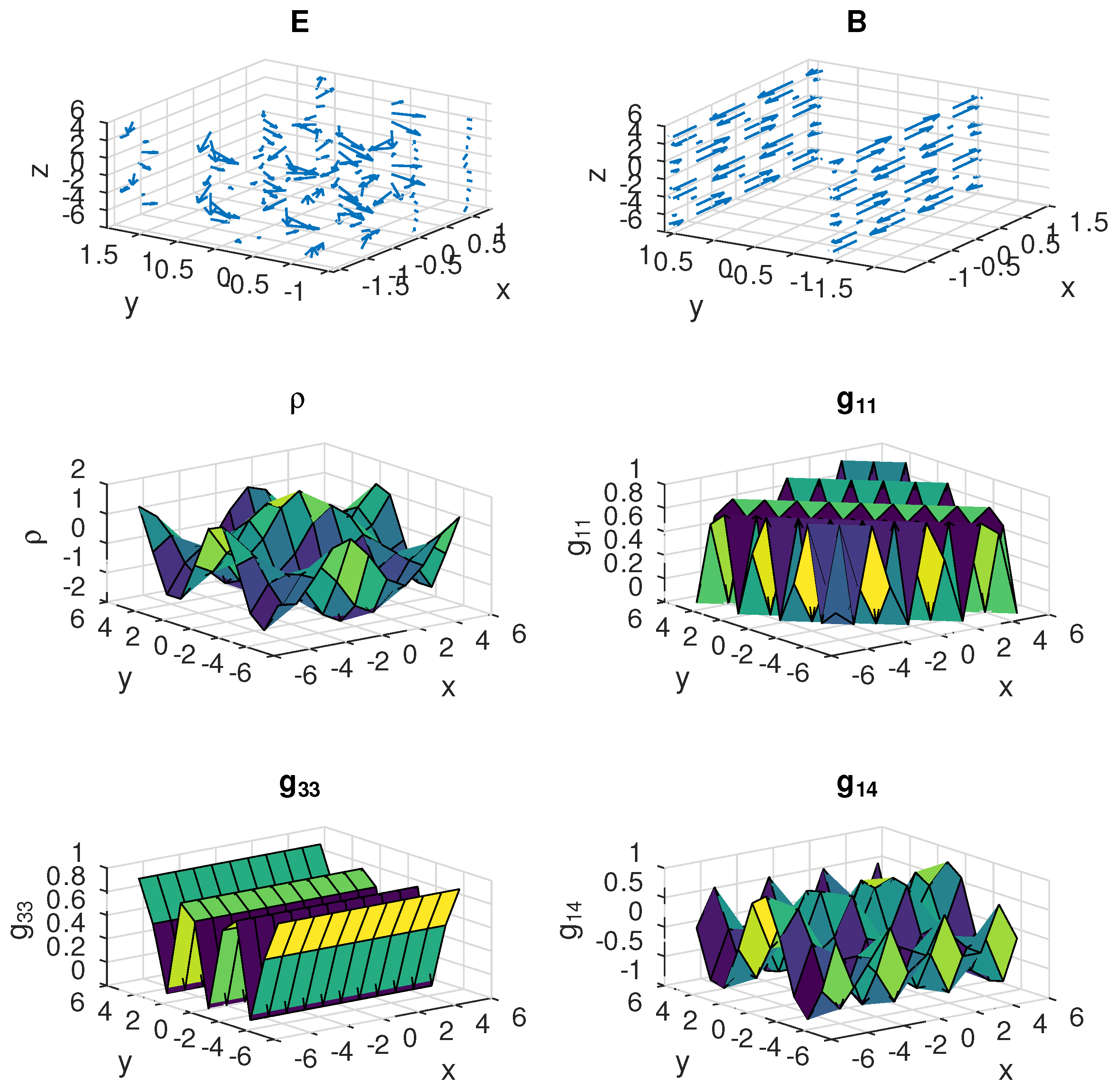
Figure 1. Illustration of the electromagnetic field, the charge density and some components of the metric tensor, when $A_0=sin(x+y-t)$, $A_1=cos(x-t)sin\left(z\right)$, $A_2=sin(y-t)cos\left(z\right)$, $A_3=cos(z-t)sin\left(x\right)$.

Figure 1. Illustration of the electromagnetic field, the charge density and some components of the metric tensor, when $A_0=sin(x+y-t)$, $A_1=cos(x-t)sin\left(z\right)$, $A_2=sin(y-t)cos\left(z\right)$, $A_3=cos(z-t)sin\left(x\right)$.

5. The Linear Maxwell’s Equations in Gaugeless Electrodynamics

5.1. The Mathematically Simplest Formulation of Maxwell’s Equation

In this section we derive the mathematically simplest formulation of Maxwell’s equation, and shall compare it against the above obtained linear Maxwell’s equation. The following derivation is based on the approach of reference [12].

In the early 20th century, it was discovered that the four Maxwell’s equations can be written as a single differential equation of the electromagnetic four-potential field $A_{\nu }$. Taking the spacetime gradient of the vector potential field yields three field types: electric, magnetic, and scalar. The role of the scalar field was not understood at the time, and it was assumed to be always zero2. There are no experimental proofs for this assumption, and it was in fact shown to lead to paradoxes [15]. In order to avoid paradoxes and to eliminate unnecessary assumptions, we allow the presence of an electromagnetic scalar field.

We use the Clifford algebra of spacetime in this section because it highlights the geometric meaning of Maxwell’s equation. An introduction to Clifford algebra can be found in the appendix. We define the differentiation operator ∂ in spacetime algebra:

$$\partial ={\gamma }_x{\displaystyle \frac{\partial }{\partial x}}+{\gamma }_y{\displaystyle \frac{\partial }{\partial y}}+{\gamma }_z{\displaystyle \frac{\partial }{\partial z}}+{\gamma }_t{\displaystyle \frac{1}{c}}{\displaystyle \frac{\partial }{\partial t}}\equiv \nabla +{\gamma }_t{\displaystyle \frac{1}{c}}{\partial }_t,$$

(42)

where $\nabla ={\gamma }_x{\displaystyle \frac{\partial }{\partial x}}+{\gamma }_y{\displaystyle \frac{\partial }{\partial y}}+{\gamma }_z{\displaystyle \frac{\partial }{\partial z}}$ and $c=1/\sqrt{{ϵ}_0{\mu }_0}$).

We define the following representation of the electromagnetic vector potential: $A\equiv (A_t{\gamma }_t,\mathbf{A})$, where $\mathbf{A}$ contains the spatial components of the vector potential.

We apply the ∂ operator to A:

$$\mathit{\partial }A=\left(-{\displaystyle \frac{1}{c}}{\partial }_t{A}_t+\nabla ·\mathbf{A}\right)+\left(-{\displaystyle \frac{1}{c}}{\partial }_t\mathbf{A}+\nabla A_t\right){\gamma }_t+\nabla \times \mathbf{A}{\mathbf{fl}}_{xyz}=$$

(43)

$$=\left(-{\displaystyle \frac{1}{c}}{\partial }_t{A}_t+\nabla ·\mathbf{A}\right)+\mathbf{B}{\mathbf{fl}}_{xyz}-\mathbf{E}{\gamma }_t$$

where the terms inside the parenthesis have scalar dimensionality, the magnetic field $\mathbf{B}$ is a spatial vector, and the electric field $\mathbf{E}$ is also a spatial vector.

Equation 43 essentially means that the spacetime derivative of $A_{\nu }$ gives the electromagnetic fields. Alternatively, the above spacetime differentiation can also be written in the following form:

$$\mathit{\partial }A=\mathit{\partial }·A_{\nu }+\mathit{\partial }\wedge A_{\nu }=S+\mathit{F}$$

(44)

where $S\equiv \left(-{\displaystyle \frac{1}{c}}{\partial }_t{A}_t+\nabla ·\mathbf{A}\right)$ contains the scalar result of dot-product differentiation, while the $\mathit{F}\equiv \mathbf{B}{\mathbf{fl}}_{xyz}-\mathbf{E}{\gamma }_t$ bi-vector is the result of wedge-product differentiation and it is known as the anti-symmetric Faraday tensor.

The actual dynamics of electromagnetism is given by the following differential equation of the $A_{\nu }$ field:

$${\partial }^{2}A=0$$

(45)

Equation 45 is the mathematically simplest formulation of Maxwell’s equation, and it is a proper field equation. It means that electric charges correspond to a certain type of electromagnetic field, and no longer have to be inserted as “external objects” into Maxwell’s equation. To see how the dynamics of electromagnetic induction and waves emerges, we firstly calculate the spacetime differential of various field components:

$$\partial \mathbf{B}{\mathbf{fl}}_{xyz}=-{\displaystyle \frac{1}{c}}{\partial }_t\mathbf{B}{\mathbf{fl}}_{txyz}+\left(\nabla ·\mathbf{B}\right){\mathbf{fl}}_{xyz}+\nabla \times \mathbf{B}{\gamma }_{xyz}^2$$

(46)

$$\partial \mathbf{E}{\mathbf{fl}}_t={\displaystyle \frac{1}{c}}{\partial }_t\mathbf{E}+\left(\nabla ·\mathbf{E}\right){\mathbf{fl}}_t+\nabla \times \mathbf{E}{\mathbf{fl}}_{txyz}$$

(47)

$$\partial S={\displaystyle \frac{1}{c}}{\partial }_{t}S{\mathbf{fl}}_t+\nabla S$$

(48)

Using the above expressions, Maxwell’s equation takes the following form:

$${\partial }^{2}A=\partial \left(S+\mathbf{B}{\mathbf{fl}}_{xyz}-\mathbf{E}{\mathbf{fl}}_t\right)=$$

(49)

$$=\left({\displaystyle \frac{1}{c}}{\partial }_{t}S-\nabla ·\mathbf{E}\right){\mathbf{fl}}_t+\nabla ·\left(S+\mathbf{B}{\mathbf{fl}}_{xyz}\right)-\left(\nabla \times \mathbf{E}+{\partial }_t\mathbf{B}\right){\mathbf{fl}}_{txyz}-\left(\nabla \times \mathbf{B}-{\partial }_t\mathbf{E}\right)$$

Equation 45 is satisfied when the terms of the above expression evaluate to zero. Let us examine the individual terms. The third and fourth terms define the induction between electric and magnetic fields: $\left(\nabla \times \mathbf{E}+{\partial }_t\mathbf{B}\right)=0$ by Faraday’s law and $\left(\nabla \times \mathbf{B}-{\partial }_t\mathbf{E}\right)=0$ by Ampere’s law of induction. Regarding first term, the $\left({\displaystyle \frac{1}{c}}{\partial }_{t}S-\nabla ·\mathbf{E}\right)=0$ condition means that ${\displaystyle \frac{1}{c}}{\partial }_{t}S=\nabla ·\mathbf{E}$, i.e. the scalar field’s time derivative is associated with the electric charge density. Specifically, the electric charge density is now given by the following field expression:

$${\displaystyle \frac{1}{c}}{\displaystyle \frac{\partial S}{\partial t}}={\mu }_{0}c\rho$$

(50)

where $\rho$ is the electric charge density.

Regarding the second term, the $\nabla ·\left(S+\mathbf{B}{\mathbf{fl}}_{xyz}\right)=0$ expression means that $\left(S+\mathbf{B}{\mathbf{fl}}_{xyz}\right)$ is a fluid-like quantity if electric fields are absent. Essentially, the $\nabla ·\left(S+\mathbf{B}{\mathbf{fl}}_{xyz}\right)=0$ expression defines how moving charges induce magnetic fields. This can be seen by noticing that $\nabla S$ defines the electric current density vector $\mathit{J}$:

$${\displaystyle \frac{\partial S}{\partial x}}={\mu }_0{J}_x,{\displaystyle \frac{\partial S}{\partial y}}={\mu }_0{J}_y,{\displaystyle \frac{\partial S}{\partial z}}={\mu }_0{J}_z$$

(51)

Upon substituting the above current density definition into the $\nabla ·\left(S+\mathbf{B}{\mathbf{fl}}_{xyz}\right)=0$ expression, the $\nabla \times \mathbf{B}={\mu }_0\mathit{J}$ induction law is obtained.

The rich dynamics of electromagnetism follows from the fact that the four terms of equation 49 are not necessarily zero individually, but in combination.

5.2. The Covariant Four-Current

The ${\partial }^{2}A=0$ Maxwell’s equation leads to equations 50 and 51, which define the charge and current densities. Therefore, the four-current $J_{\nu }$ takes the following simple form:

$$J_{\nu }=\partial S$$

(52)

Recalling that $S\equiv \partial ·A_{\nu }$, the electric four-current is defined by:

$$J_{\nu }=\partial \left(\partial ·A_{\nu }\right)$$

(53)

This results corresponds with the $\Delta A_{\nu }=J_{\nu }$ expression obtained in Section 4. It means that these two approaches are two ways of describing the same physical reality.

5.3. The Formulation of Maxwell’s Equation for Macro-Scale Analysis

In the generalized case, the scalar S field may have a microscopic wavelength components that generate electric charges and currents, as well as macroscopic wavelength components. Thus we may decompose S according to a suitably chosen wavelength threshold: $S=S_{micro}+S_{macro}$.

When the problem of interest involves a macroscopic scale, we may replace $S_{micro}$ by the usual current charge and current density parameters. Maxwell’s equation then takes the following form:

$$0={\partial }^{2}A=\left({\displaystyle \frac{1}{c}}{\partial }_{t}S-\nabla ·\mathbf{E}\right){\mathbf{fl}}_t+\nabla ·\left(S+\mathbf{B}{\mathbf{fl}}_{xyz}\right)-\left(\nabla \times \mathbf{E}+{\partial }_t\mathbf{B}\right){\mathbf{fl}}_{txyz}-\left(\nabla \times \mathbf{B}-{\partial }_t\mathbf{E}\right)=$$

(54)

$$=\left({\displaystyle \frac{1}{c}}{\partial }_t{S}_{macro}-\nabla ·\mathbf{E}\right){\mathbf{fl}}_t+\nabla ·\left(S_{macro}+\mathbf{B}{\mathbf{fl}}_{xyz}\right)-\left(\nabla \times \mathbf{E}+{\partial }_t\mathbf{B}\right){\mathbf{fl}}_{txyz}-\left(\nabla \times \mathbf{B}-{\partial }_t\mathbf{E}\right)+{\mu }_{0}J$$

where $J=\left(c\rho {\mathbf{fl}}_t+J_x{\mathbf{fl}}_x+J_y{\mathbf{fl}}_y+J_z{\mathbf{fl}}_z\right)$ is the macroscopically measured four-current.

The question arises whether there is any situation where $S_{macro}\ne 0$, i.e. whether it is a physical observable. The analysis of $S_{macro}$ in reference [12] showed that an exponentially decaying $S_{macro}$ field arises for example beyond the reflection point of acoustic phonon waves.

In fact, most works on “extended electrodynamics” theory deal with the equation 54 form of Maxwell’s equation. Representative examples are references [16,17].

5.4. The Zitterbewegung Oscillation of Electric Charges

Following the logic of preceding section, it is important to note that equation 52 applies microscopically. While a macroscopic current of electrons in a wire primarily comprises the flow of individual electron particles, the role of equation 52 becomes apparent only after sufficiently zooming in. The law of electric charge conservation can now be formulated as:

$${\displaystyle \frac{1}{{\mu }_0}}\partial ·\left(\partial S\right)=\partial ·J_{\nu }={\displaystyle \frac{\partial J_x}{\partial x}}+{\displaystyle \frac{\partial J_y}{\partial y}}+{\displaystyle \frac{\partial J_z}{\partial z}}+{\displaystyle \frac{\partial \rho }{\partial t}}=0$$

(55)

The wave equation of the scalar field S can be deduced from the charge-current conservation law:

$$\partial ·\left(\partial S\right)={\partial }^{2}S={\displaystyle \frac{{\partial }^{2}S}{\partial x^2}}+{\displaystyle \frac{{\partial }^{2}S}{\partial y^2}}+{\displaystyle \frac{{\partial }^{2}S}{\partial z^2}}-{\displaystyle \frac{1}{c^2}}{\displaystyle \frac{{\partial }^{2}S}{\partial t^2}}={\nabla }^{2}S-{\displaystyle \frac{1}{c^2}}{\displaystyle \frac{{\partial }^{2}S}{\partial t^2}}=0$$

(56)

This scalar wave equation implies that scalar waves move at the speed of light. Such light-speed circulation of electric charges is the Zitterbewegung phenomenon. Essentially, we may decompose the light-speed movement of electric charges into two perpendicular components:

$$\mathit{c}={\mathit{v}}_{\parallel }+{\mathit{v}}_{\perp }$$

where ${\mathit{v}}_{\parallel }$ is the speed of electric charge along its Zitterbewegung plane and ${\mathit{v}}_{\perp }$ is the macroscopically perceived electron speed. The light-speed circulating ${\mathit{v}}_{\parallel }$ component generates the electron spin [12].

6. The Quantum Mechanical Wavefunction Is the Lorentz-Transformed Spatial Component of the Electromagnetic Charge Oscillation

Applying the above results, we now demonstrate that the electron’s quantum mechanical wavelength is in fact the Lorentz-transformed spatial component of its Zitterbewegung oscillation. Consider an electron moving at kinetic speed v. In relation to light-speed, its speed is characterized by $\beta ={\displaystyle \frac{v}{c}},$${\gamma }_L={\left(1-{\beta }^2\right)}^{-{\displaystyle \frac{1}{2}}}$ and rapidity w defined as ${\gamma }_L=coshw$. It follows that ${cosh}^{2}w-{sinh}^{2}w=1$, $tanhw=\beta$, and $sinhw={\gamma }_L\beta$.

In the electron’s rest frame, its Zitterbewegung is a time-wise oscillation. A relativistic boost rotates the time and space axes into each other according to the following hyperbolic rotation matrix:

$$\left(\begin{array}{c}c{t}^{\prime }\\ x^{\prime }\end{array}\right)=\left(\begin{array}{cc}coshw& -sinhw\\ -sinhw& coshw\end{array}\right)\left(\begin{array}{c}ct\\ x\end{array}\right)$$

Therefore, the time-wise Zitterbewegung oscillation of the rest frame acquires a spatial oscillation component in the boosted reference frame. Specifically, the Zitterbewegung frequency of the rest frame is ${\displaystyle \frac{\omega }{2\pi }}={\displaystyle \frac{m_0{c}^2}{h}}$, and this is commonly referred to as the De Broglie frequency. The quantum mechanical wavenumber of the rest frame is: $k_0=0$. The corresponding wavenumber in the boosted frame is:

$${\displaystyle \frac{k}{2\pi }}={\displaystyle \frac{\omega }{2\pi }}{\displaystyle \frac{sinhw}{c}}-k_{0}coshw={\displaystyle \frac{\omega }{2\pi }}{\displaystyle \frac{sinhw}{c}}$$

Evaluating the right side of the above equation, we obtain:

$${\displaystyle \frac{k}{2\pi }}={\displaystyle \frac{m_0{c}^2}{h}}{\displaystyle \frac{{\gamma }_{L}v}{c^2}}$$

Rearranging the above equation, we finally obtain:

$$\hslash k=\left({\gamma }_L{m}_0\right)v=mv=p_{kinetic}$$

We recognize the above result as the basic postulate of quantum mechanics. However, it no longer needs to be a postulate: the appearing quantum mechanical wave is simply the Lorentz transformed component of the electron’s Zitterbewegung oscillation. In this sense, all quantum mechanical wavelength measurements validate the Zitterbewegung structure of the electron, with the Zitterbewegung frequency being $m{c}^2/h$.

At the same time, the relativistic $m_{relativistic}={\gamma }_L{m}_0$ mass increase directly demonstrates the circulating wave nature of the Zitterbewegung oscillation. When the circulating Zitterbewegung wave is viewed from a boosted reference frame, where the boost direction is perpendicular to the Zitterbewegung plane, the transversal relativistic Doppler effect shrinks all wavelengths by ${\gamma }_L$. This Doppler shift increases the De Broglie frequency to ${\gamma }_L{\displaystyle \frac{m_0{c}^2}{h}}$. The increase of the De Broglie frequency by a factor of ${\gamma }_L$ thus corresponds to the relativistic mass increase.

Since the quantum mechanical wavefunction is the Lorentz transformed component of the electromagnetic charge oscillation, it follows that it must be possible to express the quantum mechanical wavefunction in terms of spacetime metrics. Writing down the Dirac equation in terms of spacetime metrics has been indeed accomplished in chapter 5 of [12], and we summarize this result in Table 1. The key insight of Paul O’Hara is to use Cartan’s spinor eigenvalue method to associate the quadratic polynomial of the metric

$$\begin{array}{c}\hfill d{s}^2=g_{\mu \nu }d{x}^{\mu }d{x}^{\nu }\end{array}$$

(57)

with a spinor eigenvalue equation:

$$\begin{array}{c}\hfill ds\xi ={\gamma }_{a}d{x}^a\xi \end{array}$$

(58)

where ${\gamma }_a$ are the Clifford basis vectors of spacetime and $\xi$ is a spinor. Equation 58, in a natural way, associates spinors directly with the metrics of general relativity. As a next step, one may derive how the spinor $\xi$ of equation 58 relates to the dual of spacetime vectors.

On the one hand, each vector ${\displaystyle \frac{\partial }{\partial x^a}}$ can be mapped to a dual one-form $d{x}^a$. This produces to the second column of Table 1. On the other hand, the Dirac equation is recognized as the linearized form of the Klein-Gordon equation, where the wavefunction is defined to yield the energy eigenvalue upon time differentiation and to yield the momentum eigenvalue upon spatial coordinate differentiation. In the dual eigenvalue equation, the dual basis vectors ${\gamma }^a$ are obtained via the ${\gamma }_a=I{\gamma }^a$ assignment, where $I\equiv {\mathbf{fl}}_{txyz}$ is the Clifford pseudo-scalar whose properties are described in the appendix. It can be clearly seen from Table 1 that the $m{c}^2$ term of the Dirac equation corresponds to the ${\displaystyle \frac{\partial \psi }{\partial s}}=\left(m{c}^2\right)\psi$ eigenvalue assignment, the ℏ term is a scaling factor defined by the electromagnetic vacuum noise, and the i term corresponds to the Clifford pseudo-scalar. The Dirac equation can be therefore interpreted as a purely geometric equation, where the $m{c}^2$ term directly relates to spacetime metric. There is no need to involve any hypothetical Higgs field to explain the particle mass term.

7. The Boundary Between the Linear and Non-Linear Electromagnetic Regimes

In the context of particle physics, the linearized $\Delta A_{\nu }=J_{\nu }$ form of the Maxwell equation accounts for particle mass as electromagnetic field energy and accounts for particle spin as the magnetic moment of the circulating electromagnetic wave. Starting from the $\Delta A_{\nu }=J_{\nu }$ form of the Maxwell equation, the details of the particle mass and spin calculation can be found in reference [12] for the electron, and in reference [18] for the proton. The structural difference between an electron and a proton is just the circular versus toroidal topology difference of their Zitterbewegung oscillation, while the underlying physical equations remain the same. However, the linear $\Delta A_{\nu }=J_{\nu }$ equation cannot account for the elementary charge quantization; a different elementary charge value would be just a scaling factor adjustment for the particle mass and spin calculation. In Natural units, the elementary charge value is $e=\sqrt{\alpha }$, where $\alpha$ is the electromagnetic fine structure constant. The constant value of e and $\alpha$ indicates that they are determined by a nonlinear equation, whose solutions are only stable at a specific value of e and $\alpha$. Our results imply that the relevant nonlinear equation is the Generalized Maxwell Equation, which we derived in Section 2.

One may wonder where the boundary between the linear and generalized Maxwell equation lies. Up to now, it has been assumed that the boundary between the linear and non-linear electromagnetic regimes is at a certain electromagnetic field intensity. The proposed field intensity limit even has a name in physics: it is being referred to as the “Schwinger limit”. As we shall demonstrate in this section, the boundary between these two regimes is defined not by a threshold electromagnetic field intensity, but by a different physical parameter.

To explore the boundary between the linear and generalized Maxwell regimes, we consider magnetic flux quantization in the following paragraphs. Let A denote the vector potential experienced by the electron charge. It has the following components:

$$A\equiv V{\gamma }_t+{\mathit{A}}_{\perp }+{\mathit{A}}_{\Vert }$$

(59)

where ${\mathit{A}}_{\Vert }$ is the vector potential along the Zitterbewegung circle, ${\mathit{A}}_{\perp }$ is the axial vector potential along the kinetic speed vector, V is the electric potential, ${\gamma }_t$ is the basis vector along the time axis, and ${\gamma }_t^2=-1$.

It follows that the $eA$ expression yields the electron momentum p and energy E, which are of purely electromagnetic nature:

$$\left(E{\gamma }_t,\mathit{p}\right)=eA$$

(60)

Let $r_{orb}$ be the mean radius of the electron orbital. Its wavefunction’s continuity requires that:

$$k\left(2\pi r_{orb}\right)=n2\pi$$

(61)

where k is the wavenumber and n is a positive integer. It follows from equation 60 that the kinetic momentum defines the vector potential component along the kinetic trajectory:

$$p_{kinetic}=e{A}_{\perp }$$

(62)

It is now possible to determine the magnetic flux of an electron orbital by integrating the vector potential $A_{\perp }$ along the $d\lambda$ segments of the electron orbit:

$${\varphi }_{orb}=\oint A_{\perp }d\lambda ={\int }_0^{2\pi }{\displaystyle \frac{\hslash k}{e}}{r}_{orb}d\vartheta =k\left(2\pi r_{orb}\right){\displaystyle \frac{\hslash }{e}}=n{\displaystyle \frac{h}{e}}$$

(63)

Therefore, the magnetic flux of electron orbitals is quantized by elementary magnetic flux ${\Phi }_M=h/e$. Similarly, the $\oint A_{\parallel }d\lambda ={\displaystyle \frac{\hslash }{e}}$ relationship can be worked out as well [12,18]. Taking h as the scaling factor defined by the electromagnetic vacuum noise, we established an inverse relationship between elementary charge quantum e and elementary magnetic flux ${\Phi }_M$. Understanding the origin of e automatically yields ${\Phi }_M$, and vice versa. Working with ${\Phi }_M$ has the advantage of being directly related to the electromagnetic vector potential. For any stable charge circulation loop, the $\oint \mathit{A}·d\lambda$ expression defines a stabilized elementary quantum value, whose mathematical origin requires the generalized Maxwell regime. The vector potential can be arbitrarily large, as long as the radius of circulation is sufficiently small. Therefore, the boundary of generalized Maxwell regime is set not by some energy density threshold, but by the curvature-related $\oint \mathit{A}·d\lambda$ expression.

8. Conclusions

The present study shows that first of all electrodynamics and electromagnetism can be made into a pure geometric theory in the spirit of John Wheeler’s geometrodynamics, [19]. Maxwell’s equations correspond to an optimality condition for the variational problem, where nature wants to optimize the variation of the metric. The optimality condition then requires that the metric of the spacetime is harmonic. Furthermore, the minimal world-lines in this spacetime are given by the geodesic equation, which reduces to the familiar Lorentz law. In this sense the geometric viewpoint recreates all of classical electromagnetism. In the most general form, the geodesic equation contains additional terms which could explain the Aharonov-Bohm effect, i.e. there is a electrodynamic force present even when the electromagnetic field vanishes. Moreover, given that the electromagnetic four-potential can be affected via the four-current and the electric and magnetic fields, in principle it is possible to manipulate the local geometry of the spacetime using strong currents or electromagnetic fields.

What is however needed is the assumption of semimetricity or Weyl geometry. The present results indicate that the correct spacetime geometry for electromagnetism is the Weyl geometry with the difference to the original work by Weyl that the one-form in the eigenvalue equation is not the electromagnetic four-potential but it is the four-velocity. Given the identification $-\rho =A^{\nu }{U}_{\nu }$, it seems that the line-element in the spacetime corresponds to the strength of the charge density. Furthermore, with such an approach, electric charge seems to be directly related to the divergence of the singular metric tensor. This provides some aesthetical features into the model, as electromagnetism seems to be orthogonal to gravity in the sense that current theory of gravity is a theory based on metric compatible connections. Moreover, the wave nature of the electron becomes evident as the charge density obeys the covariant wave equation and disturbances travel at the speed of light. Our results naturally lead to interpreting the Dirac equation as a geometric equation as well, and we showed that the $m{c}^2$ term of the Dirac equation corresponds to the ${\displaystyle \frac{\partial \psi }{\partial s}}=\left(m{c}^2\right)\psi$ eigenvalue equation of the Dirac spinor field.

Clearly, the linear $\Delta A_{\nu }=J_{\nu }$ equation cannot account for the elementary charge quantization; a different elementary charge value would be just a scaling factor adjustment for the particle mass and spin calculation. We showed that the boundary between the linearized and non-linear Maxwell regimes is defined by the $\oint \mathit{A}·d\lambda$ expression. We anticipate that the analysis of the generalized Maxwell equation’s solutions may finally explain the electromagnetic fine structure constant and charge quantization.

Furthermore, assuming spacetime fluctuations in the metric tensor at Planck scales leads to randomly fluctuating electromagnetic field in vacuum. In [2], the stochastic differential equations are describing the evolution of the test particle, when both spatial and temporal dimensions are perturbed by random Brownian noise. The present study does not however argue what is the real source of the random metric perturbations, and follow-up research is needed in this respect. The model however predict the random fluctuations of the electromagnetic field at Planck scales and random creation and annihilation of charge at Planck scale due to the random covariant divergence of the electromagnetic four-potential, see also [20].

References

- J, L.; J, L. Maxwell’s equations from spacetime geometry and the role of Weyl curvature. Journal of Physics: Conference Series 2021, 1956. [Google Scholar] [CrossRef]
- J, L.; J, L. Quantum mechanics can be understood through stochastic optimization on spacetimes. Scientific Reports 2019, 9, 1–8. [Google Scholar] [CrossRef]
- L P, H. Relativistic Quantum Mechanics, 1st ed.; Springer: Dordrecht, 2015. [Google Scholar]
- J, L.; J, L. The Heisenberg Uncertainty Principle as an Endogenous Equilibrium Property of Stochastic Optimal Control Systems in Quantum Mechanics. Symmetry 2020, 12. [Google Scholar] [CrossRef]
- C, F. Stochastic Space-Time and Quantum Theory. Physical Review D 1976, 13. [Google Scholar] [CrossRef]
- D I, B. The Stochastic spaces. Particles and Nuclei 1975, 5. [Google Scholar]
- S, R. Statistical Geometry and Applications to Microphysics and Cosmology, 1 ed.; Springer: Dordrecht, 1998. [Google Scholar]
- V, V. Unified Field Theories in the First Third of the 20th Century, 1st ed.; Birkhäuser: Basel, 1994. [Google Scholar]
- H, W. Gravitation und Elektrizität. Sitzungsberichte der königlich preussischen akademie der wissenschaften zu Berlin 1918. [CrossRef]
- E, S. The Unexpected Resurgence of Weyl Geometry in late 20th-Century Physics. In: Rowe, D., Sauer, T., Walter, S. (eds) Beyond Einstein. Einstein Studies, vol 14., 1 ed.; Birkhäuser: New York, 2018. [CrossRef]
- N, R. Weyl’s Geometry and Physics. Foundations of Physics 1982, 12. [CrossRef]
- et al., K.A. Unified Field Theory and Occam’s Razor, 1 ed.; World Scientific, 2022. [CrossRef]
- O, K. Quantentheorie und fünfdimensionale Relativitätstheorie. Z. Physik 1926, 37. [Google Scholar] [CrossRef]
- R, A.; M, B.; M, S. Introduction to General Relativity, 2nd ed.; McGraw-Hill, 1975. [Google Scholar]
- G, R. The gauge non-invariance of Classical Electromagnetism. arXiv preprint 2005. [Google Scholar] [CrossRef]
- L M, H.; M, L. Extended electrodynamics and SHP theory. Journal of Physics: Conference Series 2021, 1956. [Google Scholar] [CrossRef]
- L M, H.; A S, L. Classical and extended electrodynamics. Physics Essays 2019, 32. [Google Scholar] [CrossRef]
- K.A.; et al. The proton’s and neutron’s internal structures: a simpler interpretation of modern nuclear measurements, 1 ed.; KDP, 2024. [Google Scholar]
- C W, M.; Wheeler, J. Classical Physics as Geometry: Gravitation, electromagnetism, unquantized charge, and mass as properties of curved empty space. Annals of Physics 1957, 2, 525–603. [Google Scholar] [CrossRef]
- L, P.; M A, C. The Quantum Dice, An introduction to Stochastic Electrodynamics, 1 ed.; Kluwer, 1996. [Google Scholar]