Submitted:
29 March 2025
Posted:
31 March 2025
You are already at the latest version
Abstract
The difference-from-control (DFC) test is one of the sensory discrimination methods, which is applicable to sensory evaluation in some areas including process optimization and quality assessment for foods. Thurstonian models are important and needed for any one of the sensory discrimination methods including the DFC, because it provides a useful sensory measure, Thurstonian discriminal distance, δ or d', which is theoretically independent of methods or scales used for its estimation. This paper originally derives the Thurstonian model and the maximum likelihood estimations of the model parameters for the DFC test based on a folded normal distribution. R codes for estimations and tests of δ or d' are developed and used in the paper.
Keywords:
sensory discrimination method
; difference-from-control test
; folded normal distribution
; Thurstonian discriminal distance δ or d'
1. Introduction
The difference-from-control (DFC) test is one of sensory discrimination methods. It can be used to determine degree of difference (if any) between one or more test samples and a control sample. The method is applicable to sensory evaluation in some areas including process optimization and quality assessment for foods. The ISO standard (ISO [1]) describes the application of sensory analysis in quality control (QC) using the DFC test. For more about the DFC method, see, e.g., Muñoz et al. [2]; Costell [3]; Meilgaard et al. [4]; Kemp et al. [5]; Lawless and Heymann [6], and Whelan [7].
In the DFC test, assessors are provided with an identified control sample, followed by one or more test samples. Blind controls are also included within this test. The assessors evaluate the identified control sample and the test sample(s) including blind controls, then scale how different they perceive the test sample(s) including blind controls to be from the identified control sample. There are different types of scales used for difference-from-control ratings. The rating can be done on a line or category scale. The scale may be a 9+1-point numerical scale, or a 5+1-point verbal scale, or a line scale with anchors, e.g., 0 and 100. The scales will range from 0 = “No Difference” to 9 = (or 5 =, or 100 =) “Extreme Difference”. An important characteristic of the DFC test data is that all the data are positive numbers or zero, which represent sensory intensity or distance between the test sample(s) including the blind controls and the identified control sample, regardless of the direction of the difference.
Although the DFC test has been used in various laboratory studies, to the best knowledge of the authors, there are few, if any, discussions about a Thurstonian model for the DFC test in the sensory literature. Thurstonian models are important and needed for any one of sensory discrimination methods including the DFC, because it provides a useful sensory measure, i.e., a Thurstonian discriminal distance or , which is theoretically independent of methods or scales used for its estimation (ASTM [8]).
Bradley [9] discussed Thurstonian models for some discrimination methods including the triangle, the duo-trio, and the DFC in a memorandum prepared for the General Foods Corporation. The results were published in the statistical literature (Bradley [10]). Two indices including Thurstonian and the scaled DFC measure were proposed for the DFC method. However, Bradley [10] did not indicate that the Thurstonian model is based on the folded normal distribution and how to estimate and test the indices of the model from the DFC test data. Bradley [10] mentioned that the methods of analysis for the DFC test data have not been entirely satisfactory. In the past more than 60 years since this paper was published, although there are more discussions and applications for the DFC method, the Thurstonian model for the DFC has not been discussed adequately and used widely in the sensory literature.
It should be indicated that the DFC test is also a method to determine degree of difference of two samples. Hence the DFC test can be regarded as another variant of the degree of difference (DOD) method. The conventional DOD includes three variants: the ratings of the A-Not A, the ratings of the A-Not A with reminder (A-Not AR), and the ratings of the Same-Different methods, which are commonly used and called in e.g., Aust et al. [11]; Bi [12]; Bi et al. [13]; Ennis and Rousseau [14]; Ennis and Christenson [15]; Ennis [16] (Section 8.4.1); Christensen, et al. [17]. There are three types of Thurstonian models for the three variants of the conventional DOD method. They are the Thurstonian models for the ratings of the A-Not A, the ratings of the A-Not AR, and the ratings of the Same-Different methods, which were discussed in Bi et al. [13], and Bi [18] (sections 3.3-3.5). The Thurstonian model for the DOD in Ennis and Rousseau [14]; Ennis and Christenson [15]; Christensen, et al. [17] is in fact only for the variant of the DOD, i.e., the ratings of the Same-Different method.
The main objective of this paper is to derive a Thurstonian model for the DFC method based on the folded normal distribution. The maximum likelihood estimations and statistical tests for the parameters of the model for the DFC method are also discussed and conducted. Corresponding R codes are developed and used in the paper.
2. Materials and Methods
2.1. Folded Normal Distribution for Perception of Difference Between Two Samples in the DFC Test
Let represent perception for a test sample, where follows a normal distribution with mean and variance , i.e., . Let represent perception for a control sample, where follows a normal distribution with mean and variance , i.e., . Then follows a normal distribution with parameters and , i.e., , where , .
According to the basic statistical theory (see, e.g., Read [19]), if a random variable has a normal distribution, then the absolute value of that random variable has a folded normal distribution with the same parameters. Let , then follows a folded normal distribution with the same parameters and , i.e., . In the DFC test, the assessor’s perception of the difference between the test sample and the identified control sample is just as the value of the random variable X, which follows a folded normal distribution. If the test sample is a blind control sample, then .
In the statistical literature, Leone et al. [20] first studied the properties of the folded normal distribution and provided the probability density function (pdf) with mean and variance of a folded normal distribution of as Eqs. (1)-(3). For the folded normal distribution, see also, e.g., Elandt [21], Johnson [22], Read [19], Tsagris et al. [23], and Chatterjee and Chakraborty [24].
where is the cumulative distribution function of the univariate standard normal distribution. The subscript f is used here to distinguish the mean and variance of a folded normal distribution from that of a normal distribution. Equation (1) can also be expressed as Equation (4). See, e.g., Elandt [21].
It is noted from Equation (4) that , hence we can regard as a distance between and , i.e., .
It is convenient to re-parameterize and to and σ, where and . The probability density function (pdf) of the folded normal distribution in Equation (1) can be expressed as Equation (5).
Equation (5) becomes Equation (6) when .
The cumulative distribution function (cdf) of X can be obtained as Equation (7) (see, e.g., Chatterjee & Chakraborty [24]).
where, Φ(F N) (.) denotes the cdf of the folded normal distribution. The cdf of the folded normal distribution with = 0 is as Equation (8).
The Hit (H) and False-alarm (FA) probabilities for the DFC can be expressed as Equations (9) and (10) based on Equations (7) and (8).
where i=1, …, k-1, and k is the number of the k-point numerical scale in the DFC test.
Figure 1 shows the folded normal distributions of X=|Z|=|X0-Y0| with parameters = 0 and 1, respectively, and = 2. The folded normal distribution X with parameter = 0 describes the assessor’s perception of the difference between the blind control sample and the identified control sample. The folded normal distribution X with parameter = 1 describes the assessor’s perception of the difference between the test sample and the identified control sample in the DFC test. The areas under the lines from 0 to a criterion c denote the Hit (H) and False-alarm (FA) probabilities for the DFC test.
2.2. Two Indices and Related to DFC Method
There are two indices and , which are related to the DFC method. The index ( or , is a Thurstonian discriminal distance, where , i.e., the absolute value of the difference between the expectation of and the expectation of , while the index () is a scaled DFC measure for DFC test data, where , i.e., the expectation of the absolute value of the difference between and .
It is easy to demonstrate that Equation (2) can be expressed as Equation (11), which is in fact the same as the equation provided in Bradley [10].
where and in Equation (2).
It should be noted that although Bradley [10] did not mention the folded normal distribution for the DFC test data, the DFC index in Equation (11) can be derived from Equation (2) based on the folded normal distribution for the DFC test data.
Figure 2 presents the DFC index (), as a function of () or d´ for the DFC test. Note that for smaller , while when is larger.
The R code ‘DFCf(d)’ can be used for calculation of the DFC index value(s) for a given value(s) based on Equation (5). For example, for = 0, 0.5, 1, 1.5, 2, 2.5, and 3, the corresponding = 1.1284, 1.1982, 1.3993, 1.7097, 2.1005, 2.5438, and 3.0172, respectively as below.
> DFCf(d=seq(0,3,0.5))
[1] 1.1284 1.1982 1.3993 1.7097 2.1005 2.5438 3.0172
Note that = 1.1284 when = 0. It suggests that the distribution of the DFC test data is skewed and usual tests of significance are inappropriate as warned by Bradley [10]: “Sometimes difference-from-control tests have been misinterpreted”.
The R code ‘DFCd(dfc)’ can be used for calculation of the value(s) for a given index value(s). For example, for = 1.1284, 1.1982, 1.3993, 1.7097, 2.1005, 2.5438, and 3.0172, the = 0.0, 0.5, 1.0, 1.5, 2.0, 2.5, and 3.0, respectively as below.
> DFCd(DFCf(d=seq(0,3,0.5)))
[1] 0.0 0.5 1.0 1.5 2.0 2.5 3.0
2.3. The Maximum Likelihood Estimations (MLE) of
and
from Ratings of the DFC
Equation (12) is the log-likelihood function for estimation of parameter based on the Hit (H) and False-alarm (FA) probabilities for the DFC. There are total of k parameters in the log-likelihood function in Equation (12). They are and k-1 criteria =, where i=1,..k-1, and k is the number of the k-point numerical scale in the DFC test. For the maximum likelihood estimation of parameters, a local maximum L using the R program ‘nlminb’ (R Core Team [25]) on -L is required. The R program ‘hessian’ in the R package ‘numDeriv’ (Gilbert and Varadhan [26]) can be used to estimate the co-variance matrix of the estimators of parameters δ and k-1 criteria for the DFC test.
As soon as we obtain the maximum likelihood estimation of parameter , the maximum likelihood estimation of can be obtained from Equation (11). The variance of , i.e., the variance of the estimator can be estimated using the delta method (see, e.g., Bi [18] (p51) as in Equation (13).
where in Equation (14) denotes the first derivative of Equation (11).
2.4. Ratings Data of the DFC Test
The ratings data collected from the DFC test should be summarized into a data matrix with k rows and p+1 columns, where p is the number of test samples. The first column of the data matrix contains the frequences for the blind control sample versus the identified control sample, while the other p columns contain the frequences for each of the test samples vs the identified control sample.
The DFC ratings data used in the paper are listed in Table 1. There are three test samples and one control sample. The frequencies of 5+1-point scale are presented for the blind control vs identified control and each of the 3 test samples vs control. The categories of 5+1-point scale are 0= “No difference”, 1= “Very slight difference”, 2= “Slight difference”, 3= “Moderate difference”, 4= “Large difference”, 5= “Extreme difference”.
3. Results
3.1. Maximum Likelihood Estimations (MLE) of and
The R code ‘DFCdp(x)’ can be used to estimate the parameter and variance of . The R code ‘DFCdpdfdf(x)’ can be used to estimate both the parameters and and the variances of the estimators and . The data file (x) for each test sample is a data matrix with k rows and two columns. The first column is the frequencies for the blind control sample versus identified control sample while the second column is the frequencies for the test sample versus identified control sample.
The data file ‘dfc6’ in Table 1 contains frequencies of 100 assessors’ responses for a blind control sample and 3 test samples versus a control sample.
The maximum likelihood estimations of the parameters and for the test sample 1 versus the identified control sample are 2.4168 and 2.4674, respectively. The variances of the estimators are 0.0203 and 0.0169, respectively, as below.
> DFCdp(x=dfc6[,c(1,2)])
d-prime and its variance for DFC test
[1] 2.41684014 0.02029619
> DFCdpdf(x=dfc6[,c(1,2)])
value variance
d' 2.41684 0.02029619
df 2.46740 0.01690000
> dfc6[,c(1:2)]
Blind Control vs Identified Control Test 1 vs Identified Control
5 2 10
4 5 18
3 15 34
2 17 30
1 20 2
0 41 6
The maximum likelihood estimations of the parameters and for the test sample 2 versus the identified control sample are 0.8847 and 1.3422, respectively. The variances of the estimators are 0.0390 and 0.0085, respectively.
> DFCdp(x=dfc6[,c(1,3)])
d-prime and its variance for DFC test
[1] 0.88466792 0.03896449
> DFCdpdf(x=dfc6[,c(1,3)])
value variance
d' 0.8846679 0.03896449
df 1.3422000 0.00850000
> dfc6[,c(1,3)]
Blind Control vs Identified Control Test 2 vs Identified Control
5 2 2
4 5 6
3 15 23
2 17 22
1 20 18
0 41 29
The maximum likelihood estimations of the parameters and for the test sample 3 versus the identified control sample are 2.3322 and 2.3907, respectively. The variances of the estimators are 0.0199 and 0.0161, respectively.
> DFCdp(x=dfc6[,c(1,4)])
d-prime and its variance for DFC test
[1] 2.33223946 0.01985412
> DFCdpdf(x=dfc6[,c(1,4)])
value variance
d' 2.332239 0.01985412
df 2.390700 0.01610000
> dfc6[,c(1,4)]
Blind Control vs Identified Control Test 3 vs Identified Control
5 2 15
4 5 5
3 15 46
2 17 19
1 20 10
0 41 5
3.2. Statistical Tests for or
Bi and Kuesten [27] discussed statistical testing for the Thurstonian discriminal distance or d′ based on the estimator d′ and its variance. The statistical tests include difference testing and equivalence/similarity testing for individual for a test sample and a control sample in the DFC test; difference testing, equivalence/similarity testing, and multiple comparisons for multiple for multiple test samples in the DFC test. The corresponding R codes for the statistical tests are also provided in Bi and Kuesten [27]. The statistical tests are conducted in this section using the results of the estimators and their variances obtained in section 3.1 and contained in the data file ‘alldp’.
> alldp d' v(d')
Test 1 vs Identified Control 2.4168 0.0203
Test 2 vs Identified Control 0.8847 0.0390
Test 3 vs Identified Control 2.3322 0.0199
3.1.1. Difference Test Based on Individual d′ and Its Variance
The R code ‘dpdtest(d,v)’ can be used for the difference test with the null hypothesis and the alternative hypothesis based on an individual d′ value and its variance. For example, the result of the difference test is as below for the data in the second row in the data file ‘alldp’: d′= 0.8847, variance of d′, i.e., var(d’) = 0.0390. A significant difference was found between the test sample 2 and the control sample in the DFC test with a p-value < 0.0001.
> dpdtest(d = alldp [2,1],v = alldp [2,2])
d' var(d') z p-v
[1,] 0.8847 0.039 4.479853 3.73473e-06
3.1.2. One-Sided Equivalence/Similarity Test Based on Individual d′, Its Variance, and a Specified Similarity Limit
The R code ‘dpstest(d,v, slim)’ can be used for the one-sided equivalence/similarity test with the null hypothesis and the alternative hypothesis based on an individual d′ value, its variance, and a specified similarity limit . For example, the result of the equivalence/similarity test is as below for the data in the second row in the data file ‘alldp’: d′= 0.8847, var(d’) = 0.0390, and a specified similarity limit = 1.5. Because the p-value < 0.01, significant equivalence/similarity between the test sample 2 and control sample can be claimed in terms of the equivalence/similarity limit = 1.5 at a significance level = 0.01. It means that the perceptual difference between the test sample 2 and the control sample is smaller than the specified perceptual difference in terms of Thurstonian discriminal distance d′= 1.5.
> dpstest(d = alldp [2,1],v = alldp [2,2],slim=1.5)
d' var(d') lim z p-v
[1,] 0.8847 0.039 1.5 -3.115693 0.0009175671
3.1.3. Difference Test Based on Multiple d′ Values and Their Variances
The R code ‘dstest (d, v)’ can be used to conduct a difference test with the null hypothesis and the the alternative hypothesis , i.e., if significant, at least two parameters are different for multiple d′ values and their variances. For example, for the three d′ values and their variances in ‘alldp’ for the 3 test samples vs control sample, the test results are as below. A significant difference was found among the 3 test samples in the DFC test with a p-value < 0.01.
> dstest(d=alldp[,1],v=alldp[,2])
p-value: 0
Weighted mean: 2.0689
Variance of Wm: 0.008
[1] 0.0000 2.0689 0.0080
3.2.4. Multiple Comparisons for Multiple d′ Values and Their Variances
The S-Plus program ‘multicomp’ in S-PLUS 6 (Insightful [28]) can be used for the multiple comparisons based on a vector of multiple d-prime (‘dp1’) and a co-variance matrix (‘dv1’) with a selected alpha level, e.g., alpha = 0.2. The vector and the co-variance matrix are produced as below.
>dp1<-c(T1 = alldp [1,1],T2 = alldp [2,1],T3 = alldp [3,1])
>dv1<-matrix(0,3,3)
>diag(dv1)<-alldp[,2]
> dp1
T1 T2 T3
2.4168 0.8847 2.3322
> dv1
[,1] [,2] [,3]
[1,] 0.0203 0.000 0.0000
[2,] 0.0000 0.039 0.0000
[3,] 0.0000 0.000 0.0199
Significant differences were found between test sample 1 (T1) and test sample 2 (T2) and between test sample 2 (T2) and test sample 3 (T3) as below.
> multicomp(dp1,dv1,alpha = 0.2)
80 % simultaneous confidence intervals for specified
linear combinations, by the Tukey method
critical point: 1.7151
response variable:
intervals excluding 0 are flagged by '****'
Estimate Std.Error Lower Bound Upper Bound
T1-T2 1.5300 0.244 1.110 1.950 ****
T1-T3 0.0846 0.200 -0.259 0.428
T2-T3 -1.4500 0.243 -1.860 -1.030 ****
3.2.5. Equivalence/Similarity Test Based on Two d′ Values, Their Variances, and a Specified Similarity Limit
The R code ‘s2dptest(d,v,d0)’ can be used for the two one-sided tests (TOST) with the two sets of one-sided hypotheses versus and versus for two test samples based on two estimators, e.g., and for test samples T1 and T3 and their variances. The input of the code is the two estimators and their variances, as well as an equivalence/similarity limit . The output of the code are the test statistics Z1 and Z2 and the p-values.
For example, for the data d = c(2.4168,2.3322), v = c(0.0203,0.0199), and an equivalence/similarity limit d0 = 0.5, the output is as below. Significant equivalence/similarity of T1 and T3 can be concluded with an equivalence/similarity limit of d0= 0.5 at a significance level of 0.05.
> s2dptest(d = alldp[c(1,3),1],v =alldp[c(1,3),2],d0 = 0.5)
Z1,Z2,pv1,pv2:
Test1 vs Control Test1 vs Control Test1 vs Control Test1 vs Control
2.9157 -2.0718 0.0018 0.0191
> alldp[c(1,3),]
d' v(d')
Test 1 vs Identified Control 2.4168 0.0203
Test 3 vs Identified Control 2.3322 0.0199
4. Discussion
4.1. Thurstonian Model for the DFC and the Ratings of the Same-Different
It is noted interestingly that the Hit and False-alarm probabilities for the DFC test in Eqs. (9)-(10) are the same as the Hit and False-alarm probabilities for the Same-Different method for the k-point scale when k= 2 as discussed in Kaplan et al. [29] and Bi [30]. The Hit and False-alarm probabilities for the DFC test in Eqs. (9)-(10) are the same as the Hit and False-alarm probabilities for the ratings of the Same-Different method for the k-point scale when k> 2 as discussed in e.g., Bi et al. [13]. Hence the Thurstonian model for the DFC is the same as that for the Same-Different and the ratings of the Same-Different though the DFC is different from the Same-Different and the ratings of the Same-Different in designs.
In the DFC test, assessors are provided with an identified control sample, followed by one or more test samples including blind controls. The assessor’s task is to scale how different they perceive the test sample(s) including blind controls to be from the identified control sample. In the DFC test, the possible same sample pair is only C/C1 and the different sample pair is only T/C, where T denotes test sample, C denotes control sample, and C1 denotes blind control sample.
In the Same-Different test, two products of interest (A and B) are selected. It is not necessary for the two products to be a test sample and a control sample. Assessors are presented with one of the four possible sample pairs: A/A, B/B, A/B, and B/A. The assessor’s task is to categorize the given pair of samples as same or different (ASTM [31]). For the ratings of the Same-Different, the assessor’s task is to give ratings for sureness of difference for given sample pair.
Note that the Thurstonian model in the R program ‘dod’ in the R package ‘sensR’ (Christensen, et al. [17]) is just the variant of the DOD for the ratings of the Same-Different method. Using the R program ‘dod’ in the R package ‘sensR’ and the data ‘dfc6’, the estimated d-prime is 2.391 with Std. Error 0.22211 (i.e., variance 0.2211^2 = 0.0489), which are consistent with the results (d-prime = 2.4168 with variance 0.0203) obtained by using the R code ‘DFCdp(x)’ in section 3.1 of this paper.
> library(sensR)
> dod(same=rev(dfc6[,1]),diff=rev(dfc6[,2]))
Results for the Thurstonian model for the Degree-of-Difference method
Confidence level for 2-sided profile likelihood interval: 95%
Estimates Std. Error Lower Upper
d.prime 2.391 0.2211 1.946 2.818
…
> 0.2211^2
[1] 0.04888521
4.2. Scales Used in the DFC Test
There are different types of scales used for DFC ratings. For the larger number of k in the k-point rating scales, the frequencies for some categories may be smaller or zero. It is suggested to coalesce the frequencies for larger number of k-point scale into the frequnces in a smaller number of categories. For example, transfer the 100-point scale data or 9+1-point scale data into 6-point scale or 3-point, or 2-point scale data. In theory, the parameter is independent of criteria. Hence, for a specified control sample and a specified test sample, the parameter should be unchanged by using different types of scales in theory. Note that the R codes ‘DFCdp (x)’ and ‘DFCdpdf (x)’ can be used for k-point scale data where k is larger than or equal to 2.
It is noted that the data ‘dfc3’ with 3-point ratings scale in Table 2 and the data ‘dfc2’ with 2-point ratings scale in Table 3 were summarized from the data ‘dfc6’ with 5+1-poin ratings scale in Table 1. The estimation results of the parameter for the data files ‘dfc3’ and ‘dfc2’ are as below. We can find that the estimated values for the three data files are similar and consistent.
> DFCdp(x=dfc3[,c(1,2)])
d-prime and its variance for DFC test
[1] 2.56502920 0.04819395
> dfc3[,c(1,2)]
Blind Control vs Identified Control Test 1 vs Identified Control
3 7 28
2 32 64
1 61 8
> DFCdp(x=dfc3[,c(1,3)])
d-prime and its variance for DFC test
[1] 0.84958291 0.09057446
> dfc3[,c(1,3)]
Blind Control vs Identified Control Test 2 vs Identified Control
3 7 8
2 32 45
1 61 47
> DFCdp(x=dfc3[,c(1,4)])
d-prime and its variance for DFC test
[1] 2.15764936 0.04666924
> dfc3[,c(1,4)]
Blind Control vs Identified Control Test 3 vs Identified Control
3 7 20
2 32 65
1 61 15
> DFCdp(x=dfc2[,c(1:2)])
d-prime and its variance for DFC test
[1] 2.1555582 0.0606332
> dfc2[,c(1,2)]
Blind Control vs Identified Control Test 1 vs Identified Control
1 22 62
0 78 38
> DFCdp(x=dfc2[,c(1,3)])
d-prime and its variance for DFC test
[1] 0.9064568 0.1166631
> dfc2[,c(1,3)]
Blind Control vs Identified Control Test 2 vs Identified Control
1 22 31
0 78 69
> DFCdp(x=dfc2[,c(1,4)])
d-prime and its variance for DFC test
[1] 2.30971096 0.06061473
> dfc2[,c(1,4)]
Blind Control vs Identified Control Test 3 vs Identified Control
1 22 66
0 78 34
4.3. Qualifier and Limitation of the DFC Test
As one of the sensory discrimination methods, the difference-from-control (DFC) test is applicable to sensory evaluation in process optimization and quality assessment for foods. The DFC test is applied for specific situations where a reference control is available and the goal is to determine if a noticeable difference exists. The DFC test may be used for reformulation testing, process changes, ingredient substitutions, quality control and batch consistency.
The DFC test is not appropriate when no control sample is available, understanding specific differences in depth is required, determining consumer acceptance or preference, optimizing sensory attributes, comparing multiple product variations at once (i.e., ranking test), or exploratory testing with untrained panelists. The DFC test can be more variable since panelists rate the degree of difference rather than simply identifying if a difference exists as is done for other discrimination tests (i.e., triangle, duo-trio, tetrad test). The DFC test may require a larger sample size to detect small differences reliably. It does not provide detailed profiling of sensory attributes.
5. Concluding Remarks
A Thurstonian model for the DFC test provides a useful index or to measure perceptual difference between test sample(s) and the identified control sample. This paper originally derives the Thurstonian model based on a folded normal distribution. It is demonstrated that the DFC, as a variant of the degree of difference (DOD) method, shares a common Thurstonian model with another variant of the DOD, i.e., the ratings of the Same-Different method, though the DFC and the ratings of the Same-Different are quite different sensory discrimination methods. Maximum likelihood estimates of the parameters of the model are provided. Statistical tests including different tests and equivalence/similarity tests for individual or multiple d’ values obtained from the DFC test are also conducted in this paper.
Supplementary Materials
The following supporting information can be downloaded at the website of this paper posted on Preprints.org. R codes and data files used in this paper.
Author Contributions
Conceptualization, J.B. and C.K.; software, J.B.; formal analysis, J.B.; writing— original draft preparation, J.B. and C.K.; writing—review and editing, J.B. and C.K.; visualization, J.B. All authors have read and agreed to the published version of the manuscript.
Funding
Please add: This research received no external funding.
Data Availability Statement
The original contributions presented in the study are included in the article/Supplementary Materials, further inquiries can be directed to the corresponding author.
Conflicts of Interest
The authors declare that the research was conducted in the absence of any commercial or financial relationships that could be construed as a potential conflict of interest.
References
- ISO. ISO Standard 20613: Sensory analysis — General guidance for the application of sensory analysis in quality control. Switzerland. 2019.
- Muñoz, A.M.; Civille, G.V.; Carr, B.T. Sensory Evaluation in Quality Control. New York: Van Nostrand Reinhold, 1992.
- Costell, E. A comparison of sensory methods in quality control. Food Quality and Preference 2002, 13, 341–353. [Google Scholar] [CrossRef]
- Meilgaard, M.; Civille, G.V.; Carr, B.T. Sensory Evaluation Techniques (4th ed.). Boca Raton: CRC Press., 2007.
- Kemp, S.E.; Hollowood, T.; Hort, J. Sensory Evaluation: A practical handbook. Wiley-Blackwell, UK, 2009.
- Lawless, H.T.; Heymann, H. Sensory Evaluation of Food: Principles and Practices, Second ed. Springer, New York, 2010.
- Whelan, V. J. Difference from control (DFC) test, in book: Discrimination Testing in Sensory Science: A Practical Handbook, edited by L. Rogers. 2017.
- ASTM-E2262-03; Standard Practice for Estimating Thurstonian Discriminal Distances. ASTM International: West Conshohocken, PA, USA, 2021.
- Bradley, R.A. Comparison of Different-from-control, Triangle, and Duo-trio Tests in Tasting: Comparable Expected Performance. Memorandum prepared for the General Foods Corporation, November 12. 1957.
- Bradley, R.A. Some relationship among sensory difference tests. Biometrics 1963, 19, 385–397. [Google Scholar]
- Aust, L.B.; Gacula, M.C., Jr.; Beard, S.A.; Washam II, R.W. Degree of difference test method in sensory evaluation of heterogeneous product types. Journal of Food Science 1985, 50, 511–513. [Google Scholar] [CrossRef]
- Bi, J. Statistical models for the Degree of Difference method. Journal of Food Quality and Preference 2002, 13, 31–37. [Google Scholar]
- Bi, J.; Lee, H.S.; O'Mahony, M. Statistical analysis of ROC curves for the ratings of the A-Not A and the Same-Different methods. Journal of Sensory Studies 2013, 28, 34–46. [Google Scholar] [CrossRef]
- Ennis, D.M.; Rousseau, B. A Thurstonian model for the degree of difference protocol. Journal of Food Quality and Preference 2015, 41, 159–162. [Google Scholar]
- Ennis, J.M.; Christenson, R. A Thurstonian comparison of the Tetrad and Degree of Difference tests. Journal of Food Quality and Preference 2015, 40, 263–269. [Google Scholar]
- Ennis, D.M. Thurstonian Models: Categorical Decision Making in the Presence of Noise. The Institute for Perception. Richmond, VA, USA. ISBN:9780990644606, 099064460X, 2016.
- Christensen, R.H.B; Brockhoff, B.P.; Kuznetsova, A.; Birot, S.; Stachlewska, K.A.; Rafacz, D. Package ‘sensR’. Available from: http://www.r-project.org, 2023.
- Bi, J. Sensory Discrimination Tests and Measurements: Sensometrics in Sensory Evaluation. 2nd Edition, Oxford: Wiley/Blackwell Publishing, 2015.
- Read, C.B. Folded distributions. In Encyclopedia of Statistical Sciences, Vol. 3. Edited by Kotz S. and Johnson, M.L., 1983.
- Leone, F.C.; Nelson, L.S.; Nottingham, R.B. The folded normal distribution. Technometrics 1961, 3, 543–550. [Google Scholar]
- Elandt, R.C. The Folded Normal Distribution: Two Methods of Estimating Parameters from Moments. Technometrics 1961, 3, 551–562. [Google Scholar]
- Johnson, N.L. The folded normal distribution: Accuracy of estimation by maximum likelihood. Technometrics 1962, 4, 249–256. [Google Scholar]
- Tsagris, M.; Beneki, C.; Hassani, H. On the Folded Normal Distribution. Mathematics 2014, 2, 12–28. [Google Scholar] [CrossRef]
- Chatterjee, M.; Chakraborty, A.K. A simple algorithm for calculating values for folded normal distribution. Journal of Statistical Computation and Simulation 2016, 86, 293–305. [Google Scholar]
- R Core Team. R: A language and environment for statistical computing. Vienna, Austria: R Foundation for Statistical Computing. https://www.R-project.org/, 2023.
- Gilbert, P.; Varadhan, R. Accurate numerical derivatives R package “numDeriv.” Available from: http://www.r-project.org, 2019.
- Bi, J.; Kuesten, C. Thurstonian Scaling for Sensory Discrimination Methods. Appl. Sci. 2025, 15, 991. [Google Scholar] [CrossRef]
- Insightful. S-PLUS 6. In Guide to Statistics Vol.1. for Windows; Insightful Corporation: Seattle, WA, USA, 2001. [Google Scholar]
- Kaplan, H.L.; Macmillan, N.A.; Creelman, C.D. Tables of d′ for variable-standard discrimination paradigms. Behavior Research Methods & Instrumentation 1978, 10, 796–813. [Google Scholar]
- Bi, J. Variance of d′ from the same–different method. Behavior Research Methods, Instruments, & Computers 2002, 34, 37–45. [Google Scholar]
- ASTM-E2139-05; Standard Test Method for Same-Different Test. ASTM International: West Conshohocken, PA, USA, 2018.
Figure 1.
The cdf of the folded normal distributions of X=|Z|=|X0-Y0| with = 0 and 1, respectively, and = 2.
Figure 1.
The cdf of the folded normal distributions of X=|Z|=|X0-Y0| with = 0 and 1, respectively, and = 2.
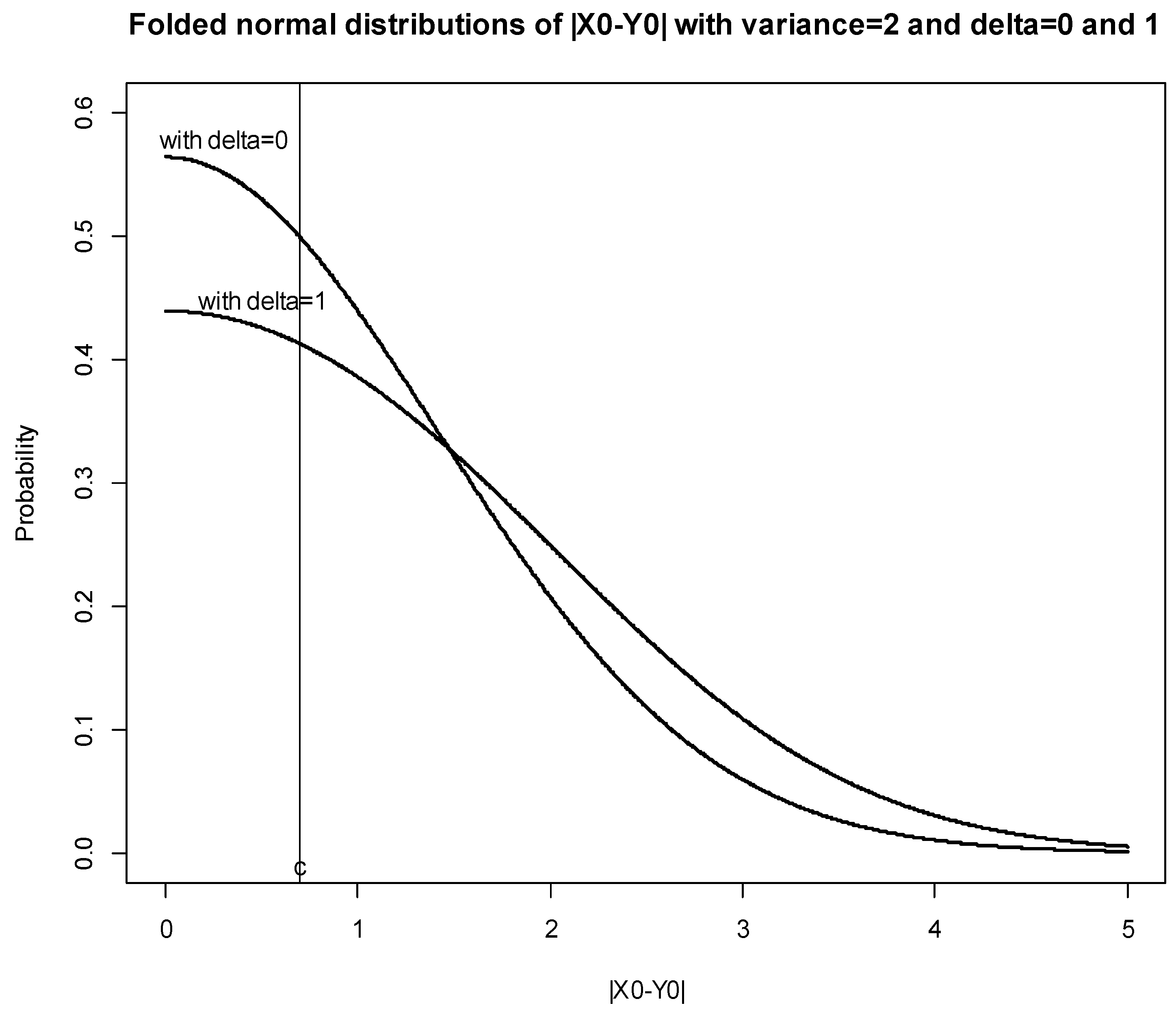
Figure 2.
Scaled DFC index as a function of Thurstonian discriminal distance
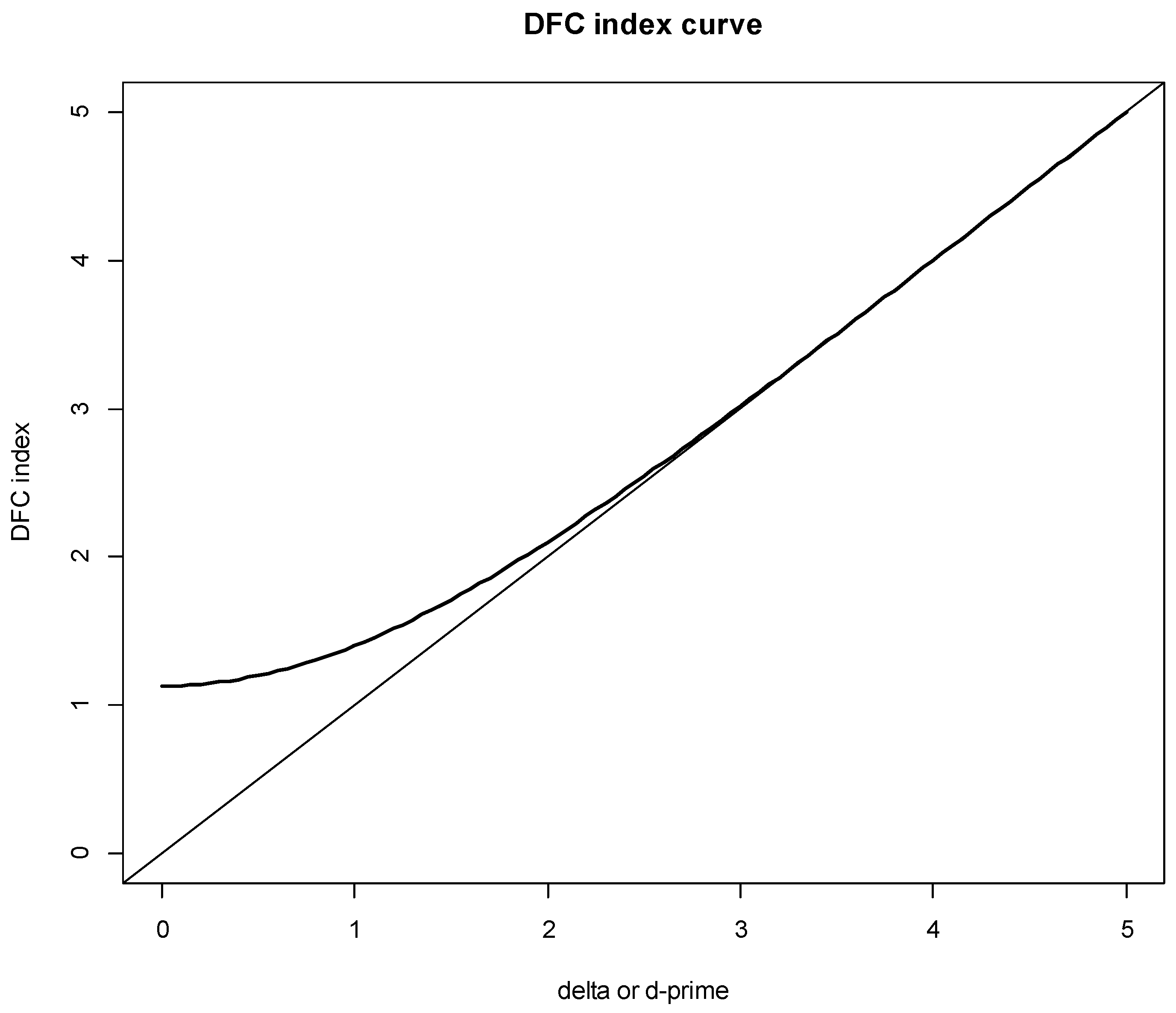

Table 1.
Frequencies of ratings with 5+1-point scale in the DFC (data ‘dfc6’).
| Categories* | Blind Control vs Identified Control |
Test sample 1 vs Identified Control |
Test sample 2 vs Identified Control |
Test sample 3 vs Identified Control |
|---|---|---|---|---|
| 5 | 2 | 10 | 12 | 15 |
| 4 | 5 | 18 | 9 | 5 |
| 3 | 15 | 34 | 43 | 46 |
| 2 | 17 | 30 | 18 | 19 |
| 1 | 20 | 2 | 8 | 10 |
| 0 | 41 | 6 | 10 | 5 |
*Note: Degree-of-difference-from-control: 0= “No difference”, 1= “Very slight difference”, 2= “Slight difference”, 3= “Moderate difference”, 4= “Large difference”, 5= “Extreme difference”.
Table 2.
Frequencies of ratings with 3-point scale in the DFC (data ‘dfc3’).
| Categories* | Blind Control vs Identified Control |
Test sample 1 vs Identified Control |
Test sample 2 vs Identified Control |
Test sample 3 vs Identified Control |
|---|---|---|---|---|
| 3 | 7 | 28 | 8 | 20 |
| 2 | 32 | 64 | 45 | 65 |
| 1 | 61 | 8 | 47 | 15 |
*Note: Degree-of-difference-from-control: 1= “Looks the same”, 2= “Not sure”, 3= “Looks the different”.
Table 3.
Frequencies of ratings with 2-point scale in the DFC (data ‘dfc2’).
| Categories* | Blind Control vs Identified Control |
Test sample 1 vs Identified Control |
Test sample 2 vs Identified Control |
Test sample 3 vs Identified Control |
|---|---|---|---|---|
| 1 | 22 | 62 | 31 | 66 |
| 0 | 78 | 38 | 69 | 34 |
*Note: Degree-of-difference-from-control: 0= “Same”, 1= “Different”.
Disclaimer/Publisher’s Note: The statements, opinions and data contained in all publications are solely those of the individual author(s) and contributor(s) and not of MDPI and/or the editor(s). MDPI and/or the editor(s) disclaim responsibility for any injury to people or property resulting from any ideas, methods, instructions or products referred to in the content. |
© 2025 by the authors. Licensee MDPI, Basel, Switzerland. This article is an open access article distributed under the terms and conditions of the Creative Commons Attribution (CC BY) license (http://creativecommons.org/licenses/by/4.0/).
Copyright: This open access article is published under a Creative Commons CC BY 4.0 license, which permit the free download, distribution, and reuse, provided that the author and preprint are cited in any reuse.


