
Submitted:
29 March 2025
Posted:
31 March 2025
You are already at the latest version
Abstract
A minimally monophyletic group is one ancestral species with four immediate descendant species. This number is optimized by the Pareto ratio as a pattern constant, which is expressed as an inverse power law at ln5/ln4 or fractal dimension 1.161. Taxa are generated by symmetry breaking of the immediate ancestron (the set of new traits of the single ancestral species shared by all immediate descendant species). Analysis used established caulistic techniques associated with descent with modification modeling, namely Shannon information with Turing sequential Bayes. The data is from taxonomic analyses using numerically enhanced classical methods of evolutionary taxonomy. Fractal modeling was done with the mathematical aid of an Artificial Intelligence leading to a quadratic model, which, because of self-similarity, is applicable to all taxonomic ranks.
Keywords:
evolution
; fractals
; hollow curves
; mirror parity
; Pareto ratio
; resilience
; symmetry breaking
; Zipf’s law
1. Introduction
Science melds theory and facts to characterize and predict the existence and effects of natural processes. For instance, in physics, theoreticians impatiently await the discoveries of experimentalists. In macroevolutionary systematics, our great collection-based institutions harbor millions of accessible samples from nature. There are commonly two methods of generating well-supported theory. Classical evolutionary taxonomy focuses on grouping and phyletically connecting taxa of various sizes, building on and adding to evolutionary theory. This is a top-down approach. Numerical taxonomy [1]) approaches from the other direction in that exact mathematical models attempt to gauge the underpinnings of processes that result in the kinds and relationships of biological diversity. Both methods bracket the complex and chaotic intersections of natural processes we see in nature. Limited by intrinsic constraints of the human psyche and physical capabilities, no one method is adequate, and the two schools of methodology are somewhat estranged. The present paper is deeply based on others preceding it. It attempts to demonstrate that classical and numerical taxonomy reveal the same truths about nature from different but integral methods. This paper uses the analytic capacities of artificial intelligence to help plumb the deeper aspects of theoretical biology [2].
Fractal Evolution
The aim of this paper is to investigate the physical foundation for the discovery in macroevolution [3] that a minimally monophyletic group (here called a “microgenus”) of one ancestral taxon has optimally four immediate descendant species, and each of these five species shares the same optimally four traits [4,5]. The generation of four descendants resulting in five total species mirroring the same traits allows modeling of this as a fractal process with a dimension of ≈ 1.161, or ln5/ln4 [6]. Note here that logarithmic fractions of a base natural or otherwise give the same result when divided, thus ln5/ln4 = log5/log4.
We will define taxa as, historically, the groups named by evolutionary taxonomists, which model evolutionary trees to reflect descent with modification, as opposed to clades conceived by cladists (most molecular systematists), which reflect analysis by common ancestry. Evolutionary taxonomists study preferentially patterns of origin versus order of origin. Taxa may be modeled as descendant from other taxa of the same rank, but clades must include all putative descendants because cladism models evolution on a classification principle, that of holophyly.
A back-grounding is necessary for descent-with-modification modeling of macroevolution, the method being fairly new and somewhat at odds with cladistics using common ancestry. The present study is actually a newly developed high-resolution phylogenetics that involves (1) multichotomous dendrograms and multi-order Markov chains using morphological and (2) now standard molecular cladograms that show paraphyly interpretable as an extant ancestor [7]. Descent-with-modification evolutionary analysis has resulted in minimally monophyletic genera (microgenera) with optimally one ancestral species and four immediate descendant species [6].
The fractal dimension of ln5/ln4 appears in systematics both in the large (Figure 1) and in the small (Figure 2). In the large, plots of numbers of species per genus (Figure 1A,B) show that the mass of genera in both vascular plants and reptiles have one to five species. The same concentration of genera per family is showing in Figure 1C, a hint of self-similarity across scale.
In the recently segregated family Streptotrichaceae [8] of 10 genera and 26 species, there are an average of 4.04 traits per species and only 2.8 species per genus, but five of the ten genera are monotypic, and, if these are down-played as remnants of larger extinct genera, then there are 4.6 species per genus as reconstructed. Additional microgenera were studied [3]. Studies of more recently established genera in the West Indies [6] showed higher numbers of species per genus. Of 36 microgenera total in [9], there were five genera with 7 6 or 7 species, 15 with 4 or 5 species, and 16 with 1 to 3 species. The six genera with five species are considered representative of the optimum, while those with fewer species have undergone some extinction, and those with greater numbers of species include secondary speciation from the immediate descendants.
In macroevolution, that which evolves is the immediate ancestron, the ca. four traits that are new to the ancestral species and transmitted entire to each of the ca. four immediate descendants. It is the immediate ancestron (Figure 3) that stabilizes each species sympatrically. Balancing the stabilizing effect of the immediate ancestron is the novon, also optimally of four species, and consists of the newly evolved traits of a descendant species. These traits are state changes of older and probably less important (for survival) characters of the ancestral species.
The generation of four items resulting in five items total (4-gets-you-5) process has a fractal dimension ≈ 1.161or ln5/ln4, which is apparently universal in macroevolution as evidenced in the study of 36 minimally monophyletic groups (microgenera) [3,4,5] (Zander 2024 a,b,c) in the hollow curves of species per genus and genera per family (Figure 1), showing self-similar distributions of 5-speciose and 5-genera taxa in many groups. This rule-of-four apparently applies to all taxonomic ranks. Significantly this includes traits, where four traits are optimal both in new traits (the novon set) and in the traits shared by ancestral species and its immediate descendants (the immediate ancestron set). This implies that taxonomic ranks are not notional but are based on real, measurable features established by evolution, namely natural selection in the context of deeper processes involving symmetry breaking [10,11]. The edge of chaos [12,13] evidenced by the logistic map is a candidate for the apparently non-linear process called speciation. The fractal dimension 1.161, or ln5/ln4, is directly related to the Pareto principle that, for instance, 20% of all people receive 80% of all income when the Pareto index α is the same as the fractal dimension 1.161. The 20/80 rule is 0.8 = 0.21/α, where α = 1.161.
Moreover, the Parteto principle is self-similar in that, of the above 20% most affluent people, 20% of them receive 80% of the money of the other wealthy folk, etc. It seems that the quasi-Zipfian sheaf [14] of evolutionarily important hollow curves presented by Zander [15] may simply approximate near the number five the Pareto ratio, which is simply but significantly an instantiation of the Pareto distribution y = x–α at 20:80 where α = 1.161(or the fractal ln5/ln4).
The change from one genus to the next is an example of symmetry breaking [16] in which the unique intersection or overlapping set of the immediate ancestron is broken, being torn away from the ancestral species into different species by the four different novons of the optimally four immediate descendant species (Figure 3). This also implies that that the immediate ancestron is basic to the rule-of-four, and provides stasis to the lineage through redundancy of the newly evolved survival traits of the ancestral species. The novons of the immediate descendants and the ancestral species’ ancestral traits are all different and provide the new exploratory traits that by organism survival provide adaptability when stasis is challenged by environmental change [6]. It is the balance of preserved and redundant traits of an ancestral species with the about an equal number of newly evolved traits that, one hypothesizes, eases speciation through mitigation of competition between allopatric species and coeval descendant species in peripheral areas (peripatry) of the ancestral species [6]. This paper is a first attempt to model this process with fractal trees.
Mirror parity is a feature of nuclear physics that provides an analogy for a similar phenomenon in evolutionary descent with modification. As diagramed (Figure 4), a lineage series of taxa, a caulon (Figure 3a-right), is an alternating set of mirrored traits, the immediate ancestron (traits other than any newly evolved traits) of the descendant being the same as the novon (newly evolved traits) of the ancestor. The symmetry of shared traits in the genus is broken during speciation by natural selection, where new species arise out of sympatry in ancestral niches.
I [15] have suggested a geometric explanation for the four descendant optimum. Plotting the area outside regular 2D geometric figures inscribed in a circle yields a hollow curve with the area coverage of each cut off portion largest among figures with sides less than five. Thus, hypothetically, the first one to five species originating peripherally around the geographic area of an ancestral species would undergo less competition between co-descendants.
Given the present fractal context, it is also possible that, prior to competitive exclusion of any more than four or five peripatric descendant species, isolation of populations in the fringes of a fractal ancestral margin (Figure 5) would restrict swamping of mutational alleles and encourage speciation through localized genetic drift under natural selection. The figure was generated by AI Claude-3.5-Sonnet to create a central mass with fringed margins modeling the geographic range of an ancestral species. It used a fractional Brownian motion algorithm, and consisted of a single enclosing line, with fractal boundary scaling at ln5/ln4 or 1.161, with smooth Catmull-Rom spline interpolation for natural curves. The original output (Supplementary material HTML 120) included adjustable roughness and detail controls. Real coastlines have fractal dimensions around 1.2 to 1.3, and actual geographic range peripheries should be similar.
The fractal dimension (Figure 5) is scaled by taking an original length L, slicing it into four equal parts, increasing the length to five equal parts, then squeezing it back into the original length by bucking the two inside parts. Thus, a length of five is shortened into a length of four with some portions buckled out of the original dimension. Mainland shoreline periphery is generated following this simple method in (Figure 6) buckling.
A diagram (Figure 7) using the equilibrium fixation index [17] p. 100 shows that more than four migrants per generation in an island situation with isolating geography strongly restricts establishment of mutations, but genetic divergence rapidly occurs with fewer migrants per generation.
Apparently evolutionary trees do not grow slowly. In a previously published caulogram of the family Streptotrichaceae, the most recent genera are fully beset with descendant species while the genera are reduced in numbers of species as they age, geologically speaking. This implies a kind of punctuated equilibrium or burst of speciation, which is similar to the theoretical avalanches of change associated with self-organized criticality [18]. This is followed by a balanced decay of the lineage through extinction and extension of the lineage terminally by addition of new genera from secondary ancestors. What supports and constrains this lineage and keeps it from going extinct or burgeoning into a massively taxon-rich unit?
2. Materials and Methods
2.1. Compilation of Data Sets and Taxonomic Groups
Standard taxonomic study uses protocols developed over 250 years of native pattern recognition coupled with homology assessment and presently rather well-developed microevolutionary theory to sort specimens into evolutionarily coherent groups as sets of taxonomic ranks. These groups provide easily analyzed small data sets that limit mistaken clustering by shared but convergent traits. These smaller groups are examined for minimally monophyletic sets of one ancestral species and a few descendant species. Ancestral species were identified by second-order Markov chains with (1) that species of the small group most similar to an outgroup (most similar species outside the group) and also (2) being most generalist (least specialized) of the ingroup. This is made more accurate by identifying the few (mostly four) traits shared by all species (among one ancestor and all immediate descendants). Such monothetic traits help define a genus, where a minimally monophyletic genus may be operationally termed a “microgenus.” The shared traits are the most newly evolved traits of the ancestor and gifted wholesale to each immediate descendant.
The microgenus is optimally a set of five species radiating from the ancestral species because speciation is rapid [4], as apparently a burst within 22 million years [6]. This is followed by speciation from the immediate descendants (secondary descendants may become central ancestors in new genera) and extinction of some of the species. Statistical support for each microgenus is by assigning each of the newly evolved traits (the novon set) of each species one Shannon informational bit, then adding the bits together and interpreting the sum as a Bayesian posterior probability using an odds chart [9]. The microgenera are strung together by connecting the ancestral species into a branching tree with gradual evolution by concatenation of the novon traits of the ancestral species. This results in a fully monophyletic tree. Molecular data may be used, particularly interpreting paraphyly as data on ancestral species and apophyly as descendant species.
2.2. Artificial Intelligence as Software
The present study used Artificial Intelligence (AI) to model mathematically processes in macroevolution (processes involving species and above) that are apparently random and based on natural selection. This is here considered a significant advance in numerical taxonomy—naming this new method high-resolution phylogenetics—because complex and calculation-onerous modeling is now possible to clarify fairly simple concepts rooted in heretofore hidden physical processes. Large-Language Model AI is rightfully viewed askance at present for its unfortunate misuse in plagiaristic composition of text and also for jumbling and misinterpretation of data obtained from the Web. In the present study, AI was mostly used as mathematical software, in which it excels, and all facts are checked with actual human publications. Interpretations of results by the AI are accepted by the author when consistent with theory, analysis, and data, and are presented as equivalent to human native pattern recognition and reasonable inference.
Most analysis, model building and image generations were done by AI Claude-3.5-Sonnet of Anthropic, Inc., with occasional use of AI Poe Assistant of Quora, Inc. Several other AIs were at first addressed for modeling macroevolution, but it the fractal images they generated were based on Mandelbrot or Julia formulae, and the resulting pretty but daunting images were not interpretable as representing anything in nature. It was Claude-3.5-Sonnet that suggested using iterated function system analysis to generate fractal trees, which proved good models of macroevolution.
Images used by this paper to model processes were generated as HTML files in htmlCanvas [19] p. 540 by the AI. Selected images are publically available at Res Botanica (see Supplementary Marterial). A fairly complete pdf version of the “chat” with the AI is also available for download online, including false starts, dead ends, wrong directions, misconstruance, and a number of interesting but discarded ideas.
Iterated function systems [20] generate fractals simply by repeating transformations, usually scaling, recursively, and converging to a fractal attractor. Patterns generated are self-similar but complex with only a small set of rules. Mapping is contractive and produces a bounded shape. The Sierpiński triangle is an example, with a fractal dimension of about 1.585, also the well-known Barnsley Fern, Cantor Set, and Koch Snowflake [21,22,23].
Dendrograms (evolutionary trees) were generated to model the ln5/ln4 tree of four branches per node apparently optimal in actual evolutionary scenarios of 36 previously studied microgenera, including the complete family Streptotrichaceae of 10 genera [8], to identify possible processes in nature. The number of branches in a microgenus may vary from none or one to four, and immediate descendants may generate secondary descendants. Because the species are monothetic, the immediate ancestral is easily discerned.
The AI used iterated function analysis to generate trees modeling at fractal dimension 1.161 the optimal four branches per node observed in morphology-based taxonomic studies. Such studies suggest that that which evolves is the immediate ancestron of about four species which provides stasis for the four novons per species that provide variability for adaptation to environmental change. The intent was to find mathematical relationships that may throw light on the underlying processes that support the continued existence of lineages, in the case of Streptotrichaceae for some 88-million years [4].
2.3. Alternative Methods
Standard common ancestry analysis using cladistics with dichotomous trees and first-order Markov chains on molecular data can identify the same extant ancestral species if paraphyly and other non-standard clues are used as indicators [7]. Cladistics alone is inadequate in that, because it has been demonstrated rather conclusively that (1) about 80% of ancestral species remain extant, and (2) depending on sampling, an ancestral species can turn up anywhere among its optimally four descendant species on a cladogram, a clade has only a 20% chance of being monophyletic, while (3) lumping different evolutionarily coherent genera together into a clade following the cladistic principle of holophyly hopelessly smudges the serial, monophyletic organization of minimally monophyletic groups (microgenera). The modern combination of a cluster-analysis form of searching for common ancestry and overemphasis on molecular traits masks information on fundamental evolutionary relationships. The present paper replaces common ancestry with descent with modification as a primary investigative tool. It is curious how often low integers and 20% and 80% appear in discussions of apparently disparate subjects; these doubtless sometimes coincidental [25].
A summary of the species per genus in the 94 genera of Pottiaceae (Bryophyta), including the now segregated Streptotrichaceae (Figure 8) shows that large numbers of very small genera are already of a size potentially that of microgenera, yet many large genera remain as evolutionary dustbins. This summary is from 1993, prior to the bloating of the family to about 108 genera by lumping descendant genera as synonyms of ancestral groups at the same rank by molecular systematists. These (Figure 8), in 1993, are taxa generated through evolutionary taxonomy, and are not clades. Cladistic analysis exacerbates the masking of microgenera by ignoring morphological traits important in evolution, and transmogrifying taxa into scientifically useless clades by lumping ancestral taxa with descendant taxa of the same rank, and usually misrepresenting clades as taxa. The present analysis focuses on descent with modification potentially reviving evolutionary taxonomy with addition of numerical methods.
3. Results
The results of this study support the value of informational entropy, particularly the work of Brooks and Wiley [10], as a factor in understanding natural processes. This study reflects data not available to these authors. Characteristic of how natural processes, including life, survive across time is an equilibrium, a balance between dissolution and elaboration. This is evident across wide scales of space and time. Examples include Edward Tryon’s [26] discovery that the exact balance of positive kinetic and potential mass energy in the universe with negative potential gravitational energy of all mass; the maintenance of maximum biological diversity through species replacement after loss, that is, Maximum Information Entropy [27]; Pareto ratio amounting to 20% yields 80% in taxonomy, equivalent to a fractal dimension of 1.161[6]; the Lotka-Volterra model for species competition; and adaptations for homeostasis maintaining physiological health in individuals. This distribution results in hollow curves when plotted (linearly, at log base one scales), and may be operative in inorganic chemistry as the Gazzarrini et al. [28] rule-of-four in inorganic chemistry, and more generally as the Constantin et al. [29] meta-law of physics.
Given recent work on fractal modeling, it should be considered that the idea of strong forces balancing positive and negative aspects of natural processes is better for stabilizing an internally and externally competitive ecosystem than natural processes that are solely aleatory in response to changing conditions. It is quite possible that fractals model a general distribution of equilibrium-bringing, sustaining processes maximizing informational entropy across scales of space and time by balancing rate and kind of extinction and multiplication of major elements in a lineage. That is, modeling an equilibrium of processes controlling decoherence of lineages by chaotic processes (edge of chaos) with the stabilizing processes of complexity theory (informational redundancy, retention of ancestral new traits in all immediate descendants). As previously suggested [9], evolution is also a process important for lineage survival acting above the species level.
Natural phenomena commonly are characterized by hollow curves, initially high on the y axis and tapering off for large values on the x-axis. The inflection point of a hollow curve can be various, but, as a whole, hollow curves have an inflection point at the number 5. This number may be considered the “average” point of inflection because it appears most frequently in empirical studies, and because ln5/ln4 ≈ 1.161, which is almost exactly the α value that generates the 20:80 Pareto rule, viz. 0.8 = 0.21/α and α = ln5/ln4. It is a natural growth rate, when x = 5 the system reaches about 63.2% completion, as derived from 1–e–1. For additional discussion see Mandelbrot [30] and West and Brown [31].
3.1. Constants
A physical constant is an experimental quantity that cannot be explained by theory. It is associated with a fundamental aspect of the structure of Nature [32]. Numbers identifying patterns emergent in complex systems, according to Claude-3.5-Sonnet (see Supplementary Materials under React25), are very similar to constants, differing only in level of predictability in variations, scale of measurement variations, and precision of possible measurement. The latter may be more a matter of categorization than fundamental differences. In this paper, the Pareto ratio is considered sufficiently descriptive of fundamental patterns that it may be considered a “pattern constant.”
Except for occasional horizontal gene transfer, evolution of already speciated groups, that is, higher taxonomic ranks, is not mediated by parallel or coordinated genetic processes similar to those investigated with population biology for microevolution. The present study suggests that the observed similarities affecting survival, resilience, and equilibrium among higher taxa is due to shared and potentially universal physical processes [14,29] associated with certain mathematical constants. One may identify universally effective but somewhat hidden closely related universals of the macroevolutionary process that may create a balanced combination of adaptation and homeostasis at lineage level.
3.1.1. The Feigenbaum Constant
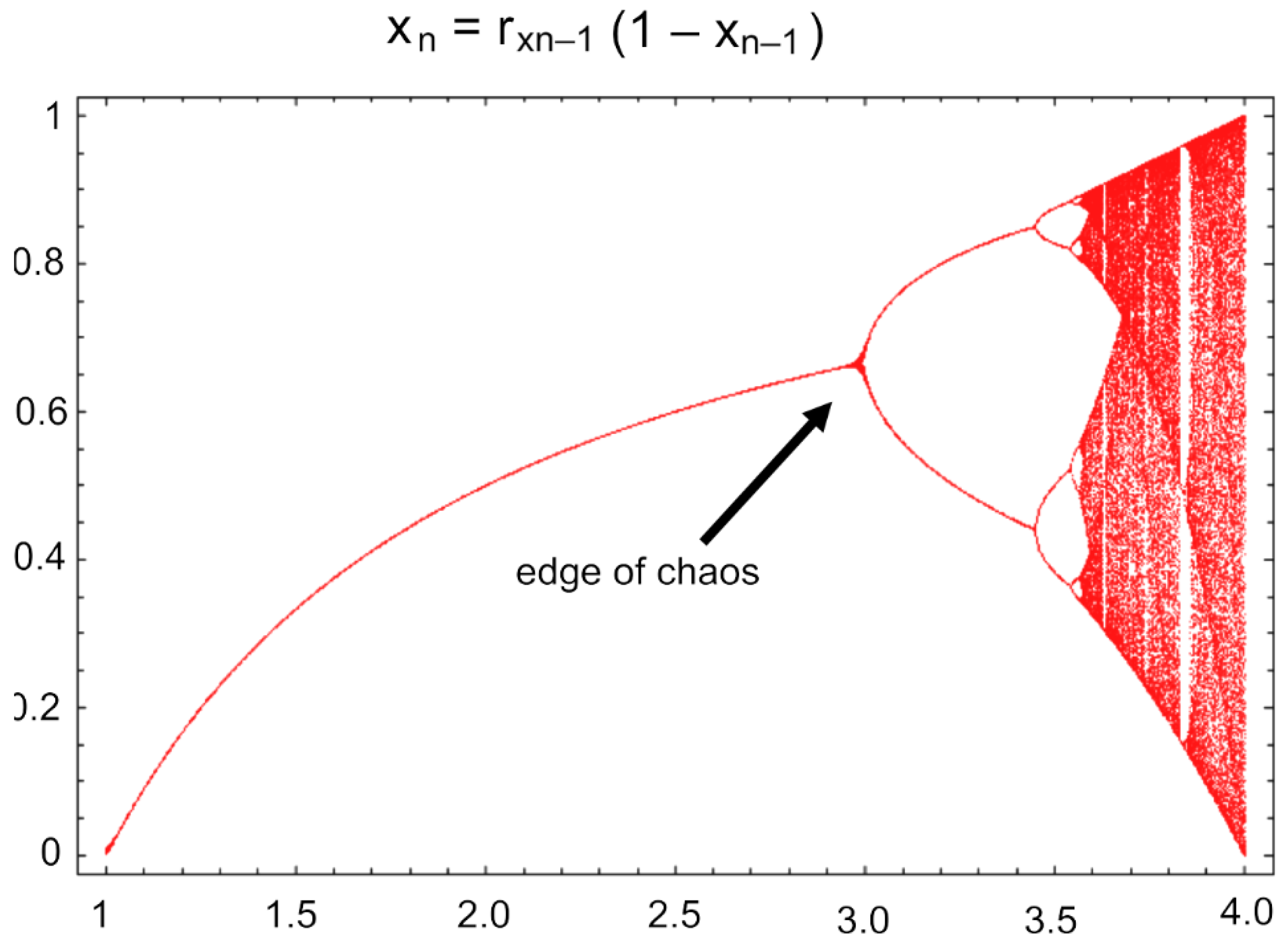
The Feigenbaum constant 4.669201609..., hereinafter 4.66, rules the logistic graph or nonlinear map in Chaos Theory [33], and is the limiting ratio of bifurcation intervals in the logistic map (Equation 1 and Figure 9). The value of the variable at the next iteration is xn+1, where x is between 0 and 1, while r is between zero and four, and controls the system. The formula is deterministic but generates complex, chaotic behavior, and is commonly used to model population dynamics, e.g., balancing reproduction and extinction associated with turbulent behavior [34,35]. The initial set of bifurcation intervals for period doubling [36] p. 116) in the logistic map (Figure 9) , where bifurcations are clearly observable and apparently becoming self-similar and not yet fully chaotic, is the “edge of chaos” [12,37]. It is associated with complex adaptive systems [38] and is here suggested as generative of lineage splitting, which given the shared immediate ancestron, involves symmetry breaking. One should note that the initial bifurcation Figure 9) results in four to eight distinct paths before rapid dissolution into chaos, possibly reflecting a Pareto ratio (2:8) in this most simple instance of logistic behavior. In addition, random Boolean networks with four or more connections between elements become chaotic [39,40].
xn+1 = rxn(1–xn)
Because even the most recent microgenera have four immediate descendant species extant, speciation is here considered abrupt (in geologic time), as a kind of punctuated equilibrium [41], being modeled by the rapid non-linear degradation of the bifurcations into chaos. Adaptation to changing circumstances is enabled by bursts of new species bearing a set of traits originating as character state changes of older, less valuable traits in the ancestral species [6].
Figure 9.
The logistic map. The “edge of chaos” is the beginning of the range of bifurcations leading to the place of total chaos. The symmetry breaking of the set of the immediate ancestron may be due to a similar nonlinear process. Adapted from Weisstein [42].
Figure 9.
The logistic map. The “edge of chaos” is the beginning of the range of bifurcations leading to the place of total chaos. The symmetry breaking of the set of the immediate ancestron may be due to a similar nonlinear process. Adapted from Weisstein [42].
3.1.2. Zipf’s Law
Mathematically, any simple mathematical operation that involves computation with increasing series of numbers (ranks, sequences) is graphically plotted as a hollow curve. The hollow curves that are high at low x values and trail off lower towards lower x values may be somewhat different depending on the mathematical operation. These are commonly generated on linear scales on the x and y axes by various formulae such as: exponential decay functions (Equation 2, where a is initial value, r as a decimal controls decay rate, and x is the period of time),
or an inverse power law (Equation 3, where the constant A > 0; x scales for height, and n > 0 is steepness of decay),
or simple logarithmic decay (Equation 4, where the constant a > 0 and determines rate of decay or growth, and +1 makes the logarithm defined for x = 0).
y = a (ln (x) + 1)
Zipf’s law [14], involving a harmonic series based on rank (1/2, 1/3, 1/4, etc.), in mathematics, parallels the fractal dimension of evolution when plotting species per genus producing a hollow curve with most area between 0 and 5 on the x axis [15]. Zipf’s formula (Equation 5, where r is numbered rank and α is a power approximating one) indicates that the rank r of a progressive series approximates the inverse of the numbered rank with a power, α, and with α approximating one. Note the similarity with the inverse power law (Equation 3). Math clue: a negative exponent is equivalent to placing the variable in the denominator, and various author replace r with x.
A hollow curve [43] illustrates the meta-law of Constantin et al. [20] which plots the frequency (in percent) of symbols and mathematical operators in physics equations. It places a dot labeled “fundamental constants” at 5 on the x-axis and 10 on the y-axis. In the paper by Constantin et al. [20], the analysis of numbers of operators (a measure of complexity) in physics equations peaks at 5 in Feynman’s work with one-third more data counts than the sets of equations with next highest complexity, and also at 5 in the Wikipedia with more than twice the counts as the next highest; for equations in the Encyclopaedia Inflationaris, equations with complexity 5 were third highest in count, with only equations with 10 and 12 operators in complexity with higher counts. The meta-law for physics formulae of Constantin et al. [20] is governed by Equation 6, where r is rank:
A similar hollow curve is present when plotting species per microgenus (Figure 2 above), and traits per species in microgenera [6]. Apparently this feature of mathematics is closely connected with actual fractal processes in nature, much as set theory models simple arithmetical relationships in nature [6].
Processes in nature that involve growth commonly involve the constant e, for which all constant growth is a scaled version of 2.7182818...., hereinafter 2.72, as a common rate. For instance, periodically more rapidly increasing a unit amount 1 over time (like compounding interest) converges on 1 becoming 2.72.
Zipf’s law and e are connected by the principle of least effort and natural information optimization. In optimizing information systems (e.g., a branching pattern) e is the optimal base for natural logarithms as it maximizes growth rate for minimal cost. Zipf’s law minimizes effort (as entropy). Together Zipf’s law and e reflect the principle of maximum information for minimum energy.
3.2.3. Fractal Representation of Macroevolution
The Pareto ratio constrains the result of the evolutionary process to the universal phenomenon of 4-gets-you-5 (generation of four items results in a total of five items) generalizable to all taxonomic ranks, including that of trait. The Pareto ratio is given by the Pareto distribution with α = 1.161 and is a “pattern constant.” The Pareto distribution is essentially the same as Zipf’s law, being the fraction 1/xα.
In that lineages are ultimately connected, the Biosphere is a fractal (Figure 10). All studied taxa, even including sets of traits, reflect a fractal dimension of ≈ 1.161, essentially that of the Pareto ratio that 20% of generators create 80% of that which is generated. In this example fractal image (Figure 10), although based on the optimal fractal dimension of ln5/ln4, here used for scaling, it is not particularly interpretable as representative of things or processes in nature. Mandelbrot [44] did suggest some relationships in his work (but none of the present bulbs, swirls and gyres can be construed to be of theoretic value. Figure 10 is not immediately interpretable as a model of evolution. Only when AI Claude-3.5-Sonnet projected a tree-like image (discussed below) using iterated function system analysis was modeling possible that reflects lineage change over time.
There are many mathematical ways of generating fractal images. The most famous is the Mandelbrot Set (Equation 7 where zn is a complex number sequentially, c is also a complex number, n is the iteration number, and z0 initiates the sequence at zero). Complex numbers are generated from pixel coordinates, and include i the square root of minus one (including zero on the imaginary y-axis).
For the Mandelbrot Set, the variable is c, for the Julia Set of fractal images the same general formula is used but the starting variable is z. Polar transformations create the spiral effects. For color effects no divergence results in black, otherwise number of iterations determine the color.
3.2.3. The Fractal Dimension and Pareto distribution
The fractal dimension is defined in practice as the log of the final number divided by the number generated from an originating number. The originating number is one, which is multiplied by the number of items generated to get x, while y is the total including the originating umber. The logarithms of these are divided, y by x, to get the fractal dimension in Equation 8. (Logarithms are powers representing, e.g., the dimensions square and cubic.)
Number of branches at a node are limited by crowding. The first recursion is the dendrogram (tree) stem, the second is the first node of four branches. Number of branches in the whole tree increase with the power of the recursion, 1 recursion for 4 branches, 2 for 16, 3 for 64, 4 for 256, etc.
In studied cases of minimally monophyletic macroevolution, the one ancestor generated four descendant species resulting in five species in the group, hence ln5/ln4. The fractal dimension of ln5/ln4, or 1.160964047..., hereinafter 1.161, which controls processes involving self-similar projection of a short list of ancestral traits along a lineage. This universal or pattern constant ensures a complex stasis by preservation of the mostly four newest traits of the ancestor by ensuring their presence in all, mostly four, immediate descendants.
This matches the ubiquity of Pareto’s principle, 20% of items generate 80% of that which is generated, based on the Pareto distribution (Equation 9). Following Equation 3, if α = 1 then the Pareto distribution is the same as the Zipf law [45], and if α = 1.161 (or ln5/ln4), then it gives the Pareto ratio of 20:80, which is the key to the proportions of ancestor to descendants in a minimally monophyletic group.
y = x–α
The AI used iterative function system to provide a fractal model (Figure 11) of an evolutionary scenario of four branches at each node, limited to four scales by a recursion depth of four. This reflected the fact that most recent (in a lineage) minimally monophyletic genera in a family lineage were largely of four immediate descendant species, implying an immediate burst of speciation. Genera with fewer descendant species apparently result from gradual extinction over the long term of these optimally 5-speciose genera, implying that four immediate descendants per ancestral species is both strongly encouraged and also strongly constrained by some process in nature, here suggested to be the Pareto pattern constant.
An example of this fractal in nature (Figure 12) is the “Weissia Probe” of Zander [6] p. 114, which analyzed Neotrichostomum and related genera in the West Indies. The genus Neotrichostomum is clearly ancestral to four other genera, two of which, Chionoloma and Tainoa, are microgenera (minimally monophyletic groups), and the other two are part of larger, unstudied groups. In the diagram, numbers refer to new traits evolved in those species (each set is a novon). The numbers of the evolutionarily active features at three different scales are within the range limited by the Pareto ratio of 20:80. Nature, given competition and extinction, does not follow scale invariance exactly [46]. The genus Neotrichostomum is ancestral to four other genera. If we fit it to a quadratic taxonomic hierarchy, perhaps it would be classified as a microsupergenus, or maybe just microsubtribus. Whether higher ranks are genuinely governed by the Pareto ratio, even locally, requires more study.
A plot of species per genus for the 36 studied microgenera (minimally monophyletic groups) (Figure 13) is similar to the expected hollow curve for large classical taxa (Figure 1, Figure 2, Figure 3, Figure 4, Figure 5, Figure 6, Figure 7 and Figure 8 ), but is truncated for few numbers of species per genus because only fairly speciose genera were analyzed for the four-gives-you-five fractal character of a microgenus (excepting the family Streptotrichaceae). It was also truncated beyond seven species per genus theoretically by the Pareto pattern constant.
Darwin’s [47] Origin of Species included only one evolutionary tree. It was intended to demonstrate series of extinctions along branching lineages. It was not dichotomous, as is a cladogram, but multichotomous, a caulogram. One feature, in particular, differs from analysis of actual lineages of descent with modification [6]. Darwin assigned the most recent nodes to have fewest branches, implying continued gradual branching of older nodes. While the most recent nodes in a real caulogram has fewest branches towards the base. Otherwise the number of branches per node, interestingly, of the two major Darwin branches, one had 22 nodes and averaged 2.9 branches per node (range 2 to 6, with mode of 4), and the other had 15 nodes and averaged 3.5 branches per node (range 2 to 5, mode of 4). Total average branches per node was 3.16. His guesswork on number of branches in speciation was pretty much spot on.
4. Discussion
4.1. Ecological Resilience
Ecological resilience can be defined [48,49] as the quantity of disturbance that an ecosystem can tolerate without altering self-organized processes and structures. Resilience may be modeled as resistance to a regime-shift including extinction through maximizing entropy [10] p. 362 in basins of attraction or alternative states as a low point in a wavy graph or ball-in-cup model [50]. Dissipative systems are not Hamiltonian, that is, they are not fully conservative of total energy, and tend to a maximum entropy or, equally of Shannon information [51]. In the context of evolutionary taxonomy, resilience is the survival of a nearly complete lineage across rather long time-scales. Modern floras are composed of taxa with at least fossils and often extant genera and species reaching back to the late Cretaceous, as exemplified by a microgeneric (descent with modification) study of the family Streptotrichaceae [3,4]. In the case of the great apes, one can use the Copernican method [52,53] to predict that the Homininea has at least a small chance of lasting another 200 kiloyears [5] with no changes in its resilience to environmental change, and has a 95 percent chance of lasting another 5,000 years.
4.2. Chaos
The past development of probabilistic methods was a major advance over deterministic formulae and laws in western science, but now chaos and complexity theory have shown that some simple iterative formulae can generate a wide range of complex values that are entirely determined at the outset but show an intrinsic order among highly elaborate and apparently chaotic results. Chaos theory is a vast subject, often well discussed in popular science literature [33,54]. Chaos is easiest exemplified by the logistic map (or quadratic map) generated (Figure 9) by iteration of a simplified equation (10):
y = rx(1 − x)
Solving (1) for y, where y = xn+1, with different values of x between 0 and 1 gives a simple range converging on 0.5, where 0.5 is termed the “attractor,” but this is true only below r ≈ 3.449 [34,54,55]. At r ≈ 3.449 continued iteration of Equation 10 gives two values, and with increasingly larger r, say 3.7, a rapid series of essentially random, or chaotic, bifurcations occurs. Above r ≈ 3.7, in the so-called “chaotic regime,” the values of y = xn+1 are totally irregular and there are no attractors. The formula above is one of the simplest that exhibits chaotic behavior. Following Sheffield [54] p. 277, the formula y = sin(xn+1)/4, where y = xn+1, has r initiating bifurcations at r = 3.4. For all different iterative formulae that exhibit a kind of chaotic graph, a “metric universal” number, ≈ 4.669, the Feigenbaum constant δ, describes the rate at which new states are introduced, that is, the ratio of intervals between bifurcations on a logistic map. Another number, ≈ 2.503..., the Feigenbaum constant α, describes the ratio of the widths of bifurcation intervals at the point of change from simple, periodic bifurcations to when they become chaotic.
The generation of bifurcations in simple single-variable iterative formulae involves a universal connection between all of these formulae. This deep universal may also govern or be implicated in individual ancestor-descendant splitting of a lineage, either at species or genus levels. It may constrain an expressed-trait morphological clock [4] similar to that assumed, and evidenced by fossils, in molecular studies. Lineages do split, and a limited enforced periodicity akin to punctuated equilibrium [56] p. 308 may promote survival of a lineage where chaotic crowding is not adaptive. The rule of four in evolution —one ancestral species and four immediate descendant species—is in part derived from the hollow curves of graphs plotted with species per genus and genera per family, these showing a preponderance of species (and genera) in groups of five. The restriction of numbers of species in a minimally monophyletic genus to five may be limited by competition during dispersal of the optimally four descendant species at the periphery of an ancestral range, as illustrated and discussed by Zander [15].
4.3. Complexity and Fractals
In addition to deeply hidden universal features of evolution that initiate and constrain splitting of a lineage, another universal process ingrained and powered by natural selection, is the fractal nature of genera with self-similarity at higher and perhaps lower taxonomic ranks. Genetic drift is an important precursor to speciation but only as influencing expressed traits tolerated during natural selection. This conservation under self-similarity is quite like the deep symmetries in physics [57,58]. The fractal pattern of evolution is that generation of four species creates five total, while generation of four genera creates five total. This is fractal evolution, with a fractal dimension ≈ 1.161 (or ln5/ln4). Fractals are complex figures similar to the logistic map but are commonly imaged by formulae with two or more formulae with multiple variables. When these are complex numbers, the quantity i, , is included. Sheffield [54] p. 278 offered a simple example:
y = (w2 +x2) + a
z = 2wx + b
Solving for y (in Equation 11) and z (in Equation 12), then replacing w and x with y and z iteratively, creates a phase-space diagram of non-periodic attractors [59] p. 113) associated with the Mandelbrot Set of fractal images that preserve structural features across scales.
Redundancy of information [33,60] that allows (1) positive survival of descendant species peripatrically, and in which an ancestral morpho-species in a minimally monophyletic group, through natural selection and genetic drift, invests all (optimally) four descendant species with the (optimally) four newly evolved traits of the ancestor. These promote survival sympatrically while the (optimally) four new traits of each descendant have selective advantage in adjacent allopatric ranges. Also, (2) survival of a lineage through geological time intervals is possible due to the rule of four which ensures abundant redundancy through continuance of survival-enhancing traits in all descendants. This taming of chaotic turbulence in evolutionary processes is discussed at length by Zander [3,4].
A theory may be advanced, then, that evolution includes two intertwined processes, (1) the splitting of lineages into ancestor and descendant, which develops newly characterized species to explore and adapt the lineage to changing environments, and (2) the protection of the immediate ancestron (the newest traits of the ancestral species) that preserve the adaptive footprint. The first process is species-based, and may be described by order of origination of species, i.e., a dichotomous tree; the second is genus-based and described by passage of sets of proven traits on a multichotomous tree. Processes are at different levels of interaction of organisms and their environment but proceed as a complex adaptive system, isomorphic with the patterns like the logistic map and fractal imagery.
In summary, decoherence of a lineage may be described by chaos theory, and coherence by complexity theory, together parsimonious of biomass and maximizing informational entropy, i.e., reducing uncertainty while protecting the survival of information through redundancy. This multiplex theory of evolution is apparently controlled by deep universal processes (Lewin, 1999: 62) at the edge of chaos [56] p. 292ff and governed by resonances and divergences in complexity theory [59] p. 116. It is obtained by numerical methods of analysis of abundant data rooted in taxonomy. One may ask what causal operation may be involved in the lineage-level evolutionary process and get “a process” as a response. The word “process” in evolution may be likened to the term “field” in physics as mathematical descriptions of actions filling space. Here I advance the Pareto ratio or pattern constant as a rather solidly based equivalent field with α the variable. We can measure gravity and electromagnetic forces and predict results and limitations but what they actually are is as yet beyond mind’s reach. We don’t even know what “distance” means, given the quantum microcosm and the space-like relativity of the macrocosm, and this not even mentioning the limitations on set theory by category theory and Gödel’s theorem [61].
The four-gets-you-five process has a fractal dimension of 1.161, which is apparently universal as evidenced in the hollow curves of species per genus and genera per family, showing self-similar distributions of 5-speciose and 5-genera taxa in many groups. The graph plots exhibit the long and broad asymptotic tail of a power law [45], which is an exponential curve that exists as a straight line if both graph axes x and y are logarithmic scales. Power laws are major sources of the self-similarity in fractal diagrams [36,44] in that, most simplistically by rescaling the variable (multiply by a constant), proportionality is preserved.
4.4. Combining the Laws
Various formulae that are associated with fractal evolution and symmetry breaking are variations on a basic identity, the inverse power law, see Equation 13, duplicated here:
If A = 1, then the inverse power law is the same as Zipf’s law when α = 1; and is the same as Constnatin’s meta-law for physics when α = 1/3; and also is the same for Pareto ratio when α = 1.161. It is probable that graphs of the results of many processes in nature [14] are simply inverse power laws with α and A as variables, including the hypothetical Pareto field that confines symmetry breaking to the immediate ancestron during speciation. The mathematical connections of α in this context is extensively discussed by Newman [45], who pointed out that power law distributions are the only distributions that appear the same no matter what scale we use. That is, power laws are scale-free, as are fractals, although it must be pointed out that some distributions are power law only in the tail. Searches for any sign that the Pareto principle is simply an optimized function of some constant in nature went unfulfilled, which indicates that α of 1.161 has a fundamental footprint in nature, even if α for the Pareto principle when fitted to some empirical data is slightly different.
4.4.1. Extinction
The above discussion is limited to speciation. Speciation is balanced by extinction. The former is apparently caused in bursts, as punctuated equilibrium [41] operating on extant taxa, but the analysis of the family Streptotrichaceae indicates that extinction is gradual [18,62] except for geologically occasional major catastrophes. The fractal model, then, is potentially the inverse of the speciation model, or a fractal dimension of ln4/5ln. Given serial steps in extinction of a microgenus, then ln3/ln2 would be next step for extinctions. The number ln2/ln1 requires division by zero, but a fractal image is possible with c = a small number near zero. Mandelbrot images generated by AI Poe Assistant using the formula z = z2 + c were all interestingly different, beautiful but not particularly informative although somewhat more compact as c approached zero. Naturalistic interpretations by the AI were fanciful. Continued research modeling extinction using the iterative function system is contemplated.
4.4.2. Common Ancestry Analysis
The present paper does not fit the standard Lakatosian Research Programme in that it uses a fairly new method and its fundamentals do have to be defended against the immediate question: “Why don’t you use phylogenetics? The differences between the present method, a numerically enhanced evolutionary taxonomy, and cladistics are given below for salient features, with further details in recently published papers [4,6,7,9].
Standard common ancestry analysis using cladistics with dichotomous trees and first-order Markov chains on molecular data is problematic. Phylogenetics is a modernized alias for a 50-year-old technology based ultimately on the original methods of numerical taxonomy (computational systematics, automatic classification), which centers on cluster analysis (now including probabilistic DNA base changes). The cladogram of dichotomous branches was long ago [1] intended as a visual aid to sorting the hierarchy of nested parentheses of names that resulted from numerical efforts as determining common ancestry.
Cladistics, as a phylogenetic technique, is simplistic because it uses eliminative induction, that is, restricting results to dichotomous trees, and because morphological data is deprecated in molecular studies by simply mapping it to the molecular tree. It is inaccurate because it is clear that ancestral species (at least since the late Cretaceous for the species studied here) are mostly extant, and there are four descendant species per ancestor, then 20 per cent of all clades are not monophyletic. In addition, common ancestry analysis cannot resolve the evolution through trait set intersection followed by symmetry breaking of the immediate ancestron. This has become destructive because taxa that that are otherwise acceptable because evolutionarily coherent are being lumped via the Classification Principle of Holophyly with ancestral taxa of the same rank. They are synonymized simply because they are descendants, creating large, evolutionarily bloated clades where all included taxa are supposedly descended from one ancestor. And it is deeply retrogressive because dichotomous trees can show no patterns characteristic of taxa, that is, elements of families, genera, and species are all clustered as pairs. (Cladogram multichotomies, when they are presented, are simply a consensus of two or more equally parsimonious cladograms, and do not show descent with modification.)
Cladistics with molecular data can identify the same extant ancestral species as determined using morphology with high-resolution phylogenetics if paraphyly and other non-standard clues are used as indicators. Molecular paraphyly has been used in the case of the clade Chionoloma to identify the ancestral species of the wrongly lumped taxa Oxystegus Hilp. and Pseudosymblepharis Broth. [7], which turned out to be well populated microgrnera.
The present paper is intended to encourage classical evolutionary taxonomy by offering new numerical methods in the context of descent with modification. This is in opposition to the general deprecation of classical evolutionary taxonomy by cladists as “traditional taxonomy,” bringing to mind painted shamans dancing around a smoky fire amid sounds of popping bladders and hoots of supplication to dark and ugly gods. Cladists have even published screeds averring the lack of scientific value of the concepts of genera [63,64] and even species [65]. To cladists, taxa, particularly genera [65], are taken as only notional and anyway unnecessary because common ancestry may be gauged by clades at all levels on a rigorously constrained dichotomous tree of common ancestry. The story goes that Wheeler said to Feynman: “I know why electrons have the same charge and the same mass.” Feynman: “Why is that?” Wheeler: “Because they are all the same electron!” [66]. By analogy, taxa are alike in being theoretically invariantly self-similar in construction. Yet they differ in their effect according to the scales at which they operate, including trait, species, genus, family, kingdom, domain, ecosystem, and biosphere. Thus, taxonomic rank is an important differentiation (see also Humphreys and Barraclough [67] and may be modeled as a distinct actor.
The core of a taxon is, however, the genus’ immediate ancestron as constrained by the Pareto ratio and whose symmetry is broken by natural selection and genetic drift, making species and genera very real entities reflecting distinct processes in nature. Suppose we were to use molecular methods with DNA bases for tracking evolution? For a minimally monophyletic group of one ancestral species and, say, four descendant species, there will potentially be five species and 10 evolutionarily informative molecular ancestral variants involved. Searching for paraphyly-apophyly pairs adequately will require abundant sampling. It is possible to go beyond simply ascribing ancestor status to a paraphyletic species by using nearest neighbor analysis, but it remains essential that morphological and molecular results are separate and match, and this means a quadratic or at least multichotomous model for both.
5. Conclusions
Some readers familiar with the details of microevolution theory may wonder how evolutionary information is shared without genetic exchange (excepting horizontal gene transfer). In self-similar processes of macroevolution, information is shared by common environmental pressures mediated by physics constants, as a goad for change and a constraint from overgrowth and crowding. The ultimate winner of maximized biodiversity is the biosphere (Figure 10 and 11). The two constants 4.66, and 1.161are involved closely with evolution as a time-wise sequence of speciation events. These universals, plus the edge of chaos, the latency of the immediate ancestron in the hollow curve, and the restrictions of the Pareto ratio, all effectively balance decoherence and fixation of species-level mutation among descendant species, and coherence and resilience by protecting and banking survival-effective traits. One can theorize that complexity processes possibly involving convergence and symmetry breaking of physics in the quasi-Zipfian context provide and control trait redundancy that serves to stabilize lineages and provide resilience over long time spans, while processes of chaos initiate and control lineage splitting. This study in fractal modeling uses accumulated data from taxonomic study to generate evolutionary trees with statistical support for morphological and molecular methods including both standard Markov chain Monte Carlo Bayes with molecular data, and Turing sequential Bayes with Shannon information for morphological data [9].
Two fractal images, Figure 10 and Figure 11, represent the ln5/ln4 dimension associated with symmetry breaking of speciation. The first, a rococo image (Figure 10) based on zn + 1 = c + with c = ln5/ln4, masks any clear analogy or modeling with natural phenomena. The other, a simple four-branching tree (Figure 11) based on simple recursions at ln5/ln4 in an iterated function system, is a good iconic model [68] fitting macroevolutionary Darwinian theory of descent with modification. What natural causes generate both the object in nature and constrain the model? It has been said that it is possible to deduce the shape of an invisible object by examining the holes left by its passage [690.The simple tree of Figure 11 may be filed by a Pareto “field” pervading all of evolution (or every process generating an inverse power law) that is no more magical (and no less) than those of electromagnetism and gravity.
One can theorize that complexity processes provide and control trait redundancy that serves to cohere lineages and provide resilience over long time spans, while chaos processes initiate and control lineage splitting. Universally effective but somewhat hidden closely related fundamental constants of the evolutionary process include the Feigenbaum constant ≈ 4.66..., ruling the logistic graph in Chaos theory, and the Fractal Dimension ≈ 1.161in complexity theory describing self-similar projection of a short list of ancestral traits along a lineage. These two universals effectively balance decoherence and fixation of species-level mutation among descendant species, and coherence and resilience by protecting and banking survival-effective traits.
The constant e plays a role in limiting growth patterns (e.g., compounding interest) while ln5/ln4 is a discrete power-law scaling. Sustainable branching patterns require a balance of these two processes. The optimal branch scale is where α = ln5/ln4. The continuous growth rate is limited by e. Together they create stable fractal patterns that efficiently balance growth rate and resources by e and Pareto limitation, respectively [70]. Trees that exceed a certain small size are unstable. According to Bochert and Slade [71]: “As soon as trees surpass a certain, relatively small size, tree structure ceases to be predictable by deterministic branching rules. Extrapolation from small to large branching systems requires the prediction of size-dependent structural changes by stochastic rules which allow for phenotypic variation, yet conserve the specific architectural model of a tree.”
In detail, each ancestor branch splits into four descendant branches in the ln5/ln4 fractal system. One may conclude then the following points:
- 4-way branching creates square-based spatial filling, or 22-fold symmetry. Thus the system models spatial filling.
-
The following conservation laws are followed,
- ○
- Area conservation: 4r2 = 1.
- ○
- Flow conservation: 4rD = 1.
- ○
- Resource distribution: 5rD = 1.
- ○
- ln4 models complete spacial filling in 2D.
- ○
- ln5 models slightly more resource demand.
- The ratio ln4:ln5 balances spatial coverage versus resource needs.
- is optimal continuous scaling.
-
Dimensional analysis,
- ○
- D1 linear chains are insufficient.
- ○
- D2 square filling is optimal for 4-way branching.
- ○
- D3 cubic space is potentially overcrowded.
- ○
- D4 hypercube is probably inefficient.
-
Scaling ratio:
- ○
- The scaling ratio, that is, how the length of the descendant branch is shorter than that of the ancestral branch, is r = e–1/α where α = ln5/ln4 ≈ 1.161. Thus r ≈ 0.423, which is optimum continuous (self-similarity) scaling.
- ○
- This is optimum because it balances flow, 4rD = 1 (4 branches preserve total flow), and resources, 5rD = 1 (5 units needed per 4 branches).
- ○
- α = ln5/ln4 ≈ 1.161 the balance between needs and flow.
-
Information optimality:
- ○
- α is the ratio of bits encoding ancestor and descendant states.
- ○
- Branching adds information: n × ln4.
- ○
- Information is lost through scaling: –n × ln5, reducing distinguishability.
- ○
- Information content is therefore negative and decreases linearly with depth (recursion), which represents increasing entropy in the system.
- ○
- Optimal rate of information loss balances system growth against system collapse.
- ○
-
Ratio ln5/ln4 balances by
- ▪
- Rate of information loss = ln5/ln4 ≈ 0.223 bits per level.
- ▪
- Total information at level n ≈ –0.223n bits.
- ○
- This leads to self-similarity and stable complexity, optimizing information compression.
Not only does the Pareto principle appear in many natural and social systems as a self-organizing principle, the ratio ln5/ln4 may be a natural optimum for branching structures were more than four branches become inefficient, and the 1.161 scaling factor represents (models) an optimal balance between diversification and resource constraints. Given the facts and above interpretations, it is possible to conclude that taxa are generated by serial symmetry breaking at fractal ln5/ln4. Given self-similarity, this applies to all taxa affected by the Pareto field. The fractal tree with four branches per node models the Pareto field, while the size and depth of the branches at fractal dimension 1.161models competition for resources when optimizing exponential growth.
Data on mathematical features of macroevolution allow investigations at the intersection of chaos and complexity theory using fractal images that reflect or even reveal certain constants of nature. Results using iterative function system methods with AI software carrying the mathematical load suggest that Pareto’s law operates to ensure a balance of stability and adaptability across taxonomic scales, including traits, species, genera and higher ranks. Evolution of demonstrably real taxa at levels higher than species [3,6] is apparently governed by universal processes of constraint and decoherence involving physical constants.
This paper hypothesizes that new genera are developed in a burst of a few million years as optimally four immediate descendant species from one ancestral species. These share the (optimally) four new traits evolved by the ancestor and parceled out exactly to all optimally four descendant species. This is mirror parity, with the four ancestral traits equally shared and newly evolved traits of each descendant obtained by state changes of old traits unused by the ancestral species. Speciation is then through symmetry breaking of the traits shared by all descendants as one or another descendant evolves new traits but keeps the newest ones it got from the ancestor. This applies as self-similarity to traits, species, genera, and even families because of self-similarity in the ln5/ln4 fractal pattern.
Funding
This research received no external funding.
Supplemental Materials
The following supporting information can be downloaded at the website of this paper posted on Preprints.org, Interactive htmlCanvas programs and copies of author-AI chats are available at https://www.mobot.org/plantscience/resbot/hid/2/originoftaxa.htm.
Institutional Review Board Statement
Not applicable.
Informed Consent Statement
Not applicable.
Data Availability
Much of the taxonomic data used in this analytic and synthetic study was previously published in the author’s other, here cited papers that had different aims. Mathematical information is otherwise complete herein, or, if only tangential, is included in the Supplementary Materials.
Acknowledgments
The contributions to this paper by Anthropic’s Artificial Intelligence Claude-3.5-Sonnet are many, but limited to mathematical analysis, pattern recognition, and literature searches. Original insights are the author’s alone, and he takes full responsibility for the work. A mostly complete transcript of the initial AI “chat” is available on Res Botanica (URL cited above). Selected interactive programs written in htmlCanvas by the AI are also available at this site. The Web site Poe, Inc. is acknowledged for its breadth of resources for virtual learning and research, and for its more than occasional use of AI Poe Assistant.
Conflicts of Interest
The author declares no conflicts of interest.
References
- Sokal, R.R.; Sneath, P.H.A. Principles of numerical taxonomy. San Francisco (CA): W. H. Freeman, San Francisco, 1963.
- Krakauer, D.C.; Collins; J.P.; Erwin, D.; Flack, J.D.; Fontana, W.; Laubichler, M.D.; Prohaska, S.J.; West, G.B.; Stadler, P.F. The challenges and scope of theoretical biology. J. Theor. Biol. 2011. [CrossRef]
- Zander, R.H. Minimally monophyletic genera are the cast-iron building blocks of evolution. Ukr. Bot. J. 2024, 81, 87–99. [CrossRef]
- Zander, R.H. Lineages of fractal genera comprise the 88-million-year steel evolutionary spine of the ecosphere. Plants 2024, 13, 1559. [CrossRef]
- Zander, R.H. The steel evolutionary spine revisited, with implications and consequences. Contemporary Research and Perspectives in Biological Science Vol. 1. 2024, Sept.,154–185. [CrossRef]
- Zander, R.H. Fractal Evolution, Complexity and Systematics. Zetetic Publications, St. Louis, 2023.
- Zander R.H. Integrative systematics with structural monophyly and ancestral signatures: Chionoloma (Bryophyta). Academia Biology 2024, 2. [CrossRef]
- Zander, R.H. Macroevolutionary Systematics of Streptotrichaceae of the Bryophyta and Application to Ecosystem Thermodynamic Stability, ed. 2. Zetetic Publications, St. Louis, 2018.
- Zander, R.H. Evolutionary leverage of dissilient genera of Pleuroweisieae (Pottiaceae) evaluated with Shannon-Turing analysis. Hattoria 2021, 12: 9–25.
- Brooks, D.R.; Wiley, E.O. Evolution as Entropy: Toward a Unified Theory of Biology. University of Chicago Press, Chicago. 1988.
- Ellis, G.F.R.; Di Sia, P. Complexity theory in biology and technology: broken symmetries and emergence. Symmetry 2023, 15, 1945. [CrossRef]
- Packard, N.H. Adaptation towards the Edge of Chaos. University of Illinois at Urbana-Champaign, Center for Complex Systems Research. Urbana, Illinois, 1988.
- Strogatz, S.H. Nonlinear Dynamics and Chaos: With Applications to Physics, Biology, Chemistry and Engineering. Addison-Wesley, Reading, Mass., U.S.A. 1994.
- Aitchison, L.; Corradi, N.; Latham, P.E. Zipf’s Law arises naturally when there are underlying, unobserved variables. PLoS Comput. Biol. 2016, 12, 12. e1005110. [CrossRef]
- Zander, R.H. Geometric models of speciation in minimally monophyletic genera using High-Resolution Phylogenetics. Plants 2025, 14, 530. [CrossRef]
- Krakauer, D.C. Symmetry–simplicity, broken symmetry–complexity. Interface Focus 2023, 13, (20220075), 1–6. [CrossRef]
- Hartl, D.L. A Primer of Population Genetics and Genomics. Oxford University Press, Oxford, 2020.
- Plotnick, R.E.; Sepkoski, J.J., Jr.. A multiplicative multifractal model for originations and extinctions. Paleobiology 2001, 27, 126–139.
- Ruvalcaba, Z.; Boehm, A. Murach’s HTML5 and CSS3. Training and Reference. Mike Murach & Associates, Fresno, California, 2012.
- Barnsley, M.F.; Demko, S. Iterated functions systems and the global construction of fractals. Proc. R. Soc. London. A 1985, 399, 243–275. [CrossRef]
- Barnsley, M. Fractals Everywhere. Academic Press, New York, 1988.
- Barnsley M.F.; Vince, A. The chaos game on a general iterated function system. Ergodic Theory and Dynamical Systems. 2011, 31,1073–1079. [CrossRef]
- Hutchinson, J.E. Fractals and self similarity. Indiana University Math. J. 1981, 30, 713–747. [CrossRef]
- Guy, R.K. The strong law of small numbers. Amer. Math. Monthly 1988, 95, 697–712.
- Tryon, E. Is the universe a vacuum fluctuation? Nature 1973, 246, 396–397. [CrossRef]
- Harte, J.; Newman, E.A. Maximum information entropy: a foundation for ecological theory. Trends in Ecology & Evolution 2014, 29, 384–389. [CrossRef]
- Gazzarrini, E.; Cersonsky, R.K.; Bercx, M.; Adorf, C.S.; Marzari, N. The rule of four: anomalous distributions in the stoichiometries of inorganic compounds. NPJ Comput. Mater. 2024, 10, 73.
- Constantin, A.; Bartlett, D.; Desmond, H.; Ferreira, P.G. Statistical patterns in the equations of physics and the emergence of a meta-law of nature. Arxiv 2024, arXiv:2408.11065.
- Mandelbrot, B. The Pareto-Lévy Law and the Distribution of Income. International Economic Review, 1960,1, 79–106.
- West, G.B.; Brown, J.H. Life’s Universal Scaling Laws. Physics Today 2004, 57, 36–43. [CrossRef]
- Barrow, J. D. The Constants of Nature. Pantheon Books, New York, 2002.
- Gleick, J. Chaos: Making a New Science. Penguin Books, New York, 1987.
- Infeld, E.; Rowlands. G. Nonlinear Waves, Solitons and Chaos. Cambridge University Press, New York, 2000.
- Pimm, S. L. The complexity and stability of ecosystems. Nature 1984. 307: 321–324.
- Schroeder, M. Fractals, Chaos, Power Laws, Minutes from an Infinite Paradise. W. H. Freeman, New York, 1991.
- Hastings, A.; Powell, T.. Chaos in a three-species food chain. Ecology 1991, 72, 896–903. [CrossRef]
- Bak, P.; Tang, C.; Wiesenfeld, K. “Self-organized criticality”. Physical Review A 1988, 38, 364–374. [CrossRef]
- Kauffman, S. A. Origins of Order: Self-Organization and Selection in Evolution. Oxford University Press, Oxford, 1992.
- Lewin, R. Complexity: Life at the Edge of Chaos. University of Chicago Press, Chicago, 1999.
- Eldredge, N. Time Frames: The Rethinking of Darwinian Evolution and the Theory of Punctuated Equilibria. Simon and Schuster, New York, 1985.
- Weisstein, E. W.. “Logistic Map.” From MathWorld--A Wolfram Web Resource. 2025. https://mathworld.wolfram.com/LogisticMap.html Viewed 8 March 2025.
- Wilkins, A. The laws of physics appear to follow a mysterious mathematical pattern. New Scientist 2024, 21 October 2024. https://www.newscientist.com/article/2452341-the-laws-of-physics-appear-to-follow-a-mysterious-mathematical-pattern/ Viewed 4 March 2025.
- Mandelbrot, B.B. The Fractal Geometry of Nature. Updated and augmented. W. H. Freeman and Company, New York, 1983.
- Newman, M.E.J. Power laws, Pareto distributions, and Zipf’s law. Contemporary Physics 2005, 46, 323–351.
- Newberry, M. Art and science illuminate the same subtle proportions in tree branches. The Conversation 2025, 11 February 2025 https://theconversation.com/art-and-science-illuminate-the-same-subtle-proportions-in-tree-branches-247967.
- Darwin, C. The Origin of Species by Means of Natural Selection, or the Preservation of Favoured Races in the Struggle for Life. Washington Square Press, New York. 1963 Edition, 1859.
- Gunderson, L.H. Ecological resilience—In theory and application. Ann. Rev. Ecol. Syst. 2000, 31, 425–439.
- Holling, C.S. Resilience and stability of ecological systems. Ann. Rev. Ecol. Syst. 1973, 4, 1–23.
- Ludwig, A.K.; Barnes, C.D.; Fogart,y D.; Fowler, J.A.; Hogan, I.F.E.; Johnson, J.E.; Twidwell, D. Ecological Resilience. Plant and Soil Sciences eLibrary Lessons https://passel2.unl.edu/view/lesson/d6c3e24cbc7e 2020. Accessed Dec. 28, 2025.
- Weber, B.H.; Depew, D.J.; Smith, J.D., eds. Entropy, Information, and Evolution: New Perspectives on Physical and Biological Evolution. MIT Press, Cambridge, Massachusetts, 1990.
- Gott, J.R. Time Travel in Einstein’s Universe. Houghton Mifflin, New York, 2001.
- Poundstone, W. The Doomsday Calculation. Little, Brown Spark, New York, 2019.
- Sheffield, C. Borderlands of Science. Baen Books, Riverdale New York, 1999.
- Lurie, R.M. “Classic Logistic Map” Heikki Ruskeepää 2011. Wolfram Demonstrations Project. https://demonstrations.wolfram.com/ClassicLogisticMap/ Accessed 2 Feb. 2025.
- Waldrop, M.M. Complexity: The Emerging Science at the Edge of Order and Chaos. New York, Simon and Schuster, 1992.
- Gross, D.J. The role of symmetry in fundamental physics, Proc. Natl. Acad. Sci. U.S.A. 1996, 93, 14256–14259. [CrossRef]
- Wegsman, S. How Noether’s theorem revolutionized physics. Quanta Newsletter Feb. 7, 2025. https://www.quantamagazine.org/how-noethers-theorem-revolutionized-physics-20250207/ Viewed February 27, 2025.
- Nicolis G.; Prigogine I. Exploring Complexity: An Introduction. W.J.H. Freeman and Company, New York, 1989.
- Gleick, J. The Information, A History, A Theory, A Flood. Pantheon Books, New York, 2011.
- Kline, M. Mathematics: The Loss of Certainty. Oxford University Press, Oxford, 1980.
- Hughes, B.D. Reed, W.J. A problem in paleobiology. arXiv.physics/0211090V1 [physics.bio-oph] 2002. 20 Nov. 2002. https://arxiv.org/abs/physics/0211090v1 Viewed 14 March 2025.
- Stevens, P.F. The genus concept in practice: but for what practice? Kew Bull. 1985, 40, 457–465.
- Stevens, P.F. Why do we name organisms? Some reminders from the past. Taxon. 2002, 51, 11–26. [CrossRef]
- Humphreys, A.M.; Linder, H.P. Concept versus data in delimitation of plant genera. Taxon 2009, 58, 1054–1074.
- Mishler, B.D. What, if Anything, are Species? CRC Press, Boca Raton, Florida, 2021.
- Feynman, R. Nobel Lecture. Nobel Foundation, 1965. http://www.nobelprize.org/nobel_prizes/physics/laureates/1965/feynman-lecture.html.
- Humphreys, A.M.; Barraclough, T.G. The evolutionary reality of higher taxa in mammals. Proc. Roy. Soc. B 2014, 281, 20132750. [CrossRef]
- Harré, R. The Philosophies of Science. An Introductory Survey. Oxford University Press, Oxford, 1972.
- Hughes, M. The Gist Hunter. Nightshade Books, New York, 2014.
- West, G.B.; Brown, J.H.; Enquist, B.J. A general model for the structure and allometry of plant vascular systems. Nature 1999, 400(6745), 664–667. [CrossRef]
- Borchert, R.; Slade, N.A.. Bifurcation ratios and the adaptive geometry of trees. Bot. Gaz. 1981, 142, 304–401.
Figure 1.
Graphs showing concentration of one to five species or genera. A. Species per genus in vascular plants. B. Species per genus in reptiles. C. Genera per family in angiosperms as a group (after Zander [3]). The hollow curves imply deep processes characterized by formulae involving series, exponents and/or symmetry breaking, expressed in the Pareto ratio of 20/80.
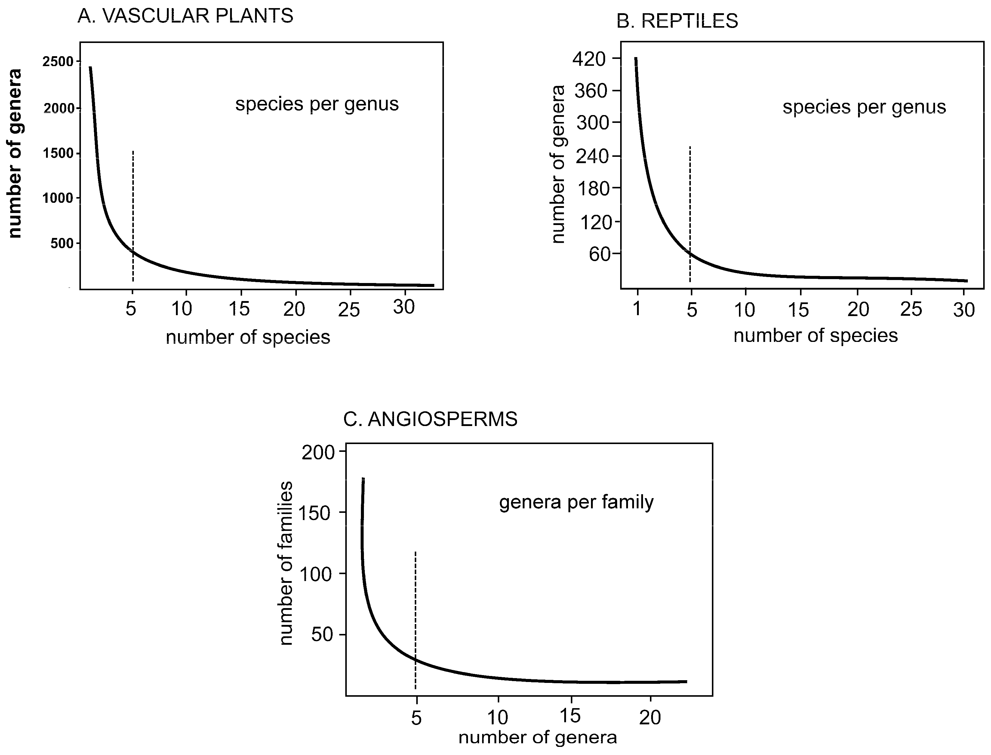
Figure 2.
Graph of 366 analyzed microgenera showing numbers of species per genus. Five is optimum, less than five undergoing to extinction, more than five have secondary speciation from immediate descendants. More than seven are absent due to Pareto ratio.
Figure 2.
Graph of 366 analyzed microgenera showing numbers of species per genus. Five is optimum, less than five undergoing to extinction, more than five have secondary speciation from immediate descendants. More than seven are absent due to Pareto ratio.
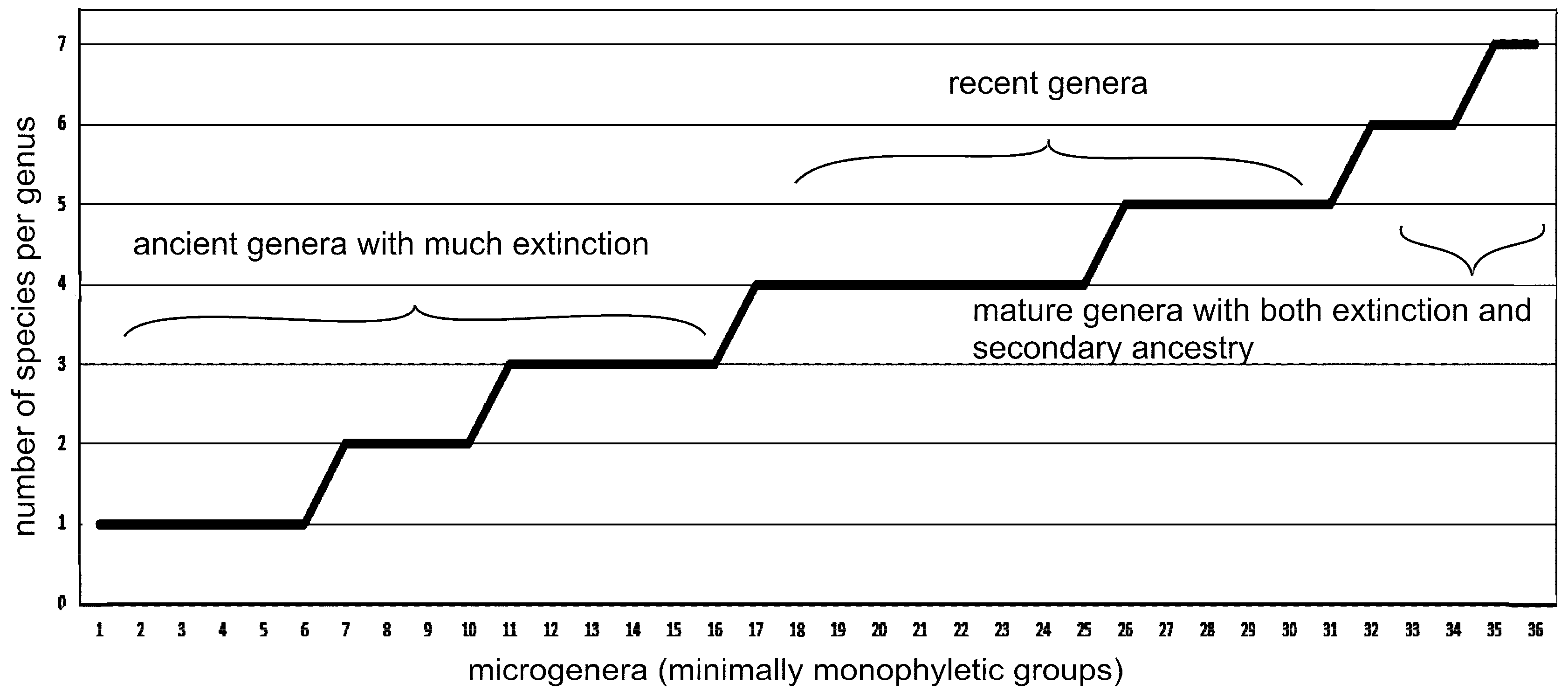
Figure 3.
Active elements of macroevolution and symmetry breaking in caulistic diagrams. (Left) A simple three-species caulon. The ancestral species contributes its novon (set of the ancestor’s newly evolved traits) entire to the descendant species in which that same set is called the immediate ancestron, while the descendant species generates its own novon from less important characters in the ancestron. (Right) A five-genus caulogram. Five minimally monophyletic genera each of five species in which the shared immediate ancestron is colored the same. Each genus has optimally five identical immediate ancestrons. The change from one genus to the next is an example of symmetry breaking. Some genera overlap due to crowding in the figure.
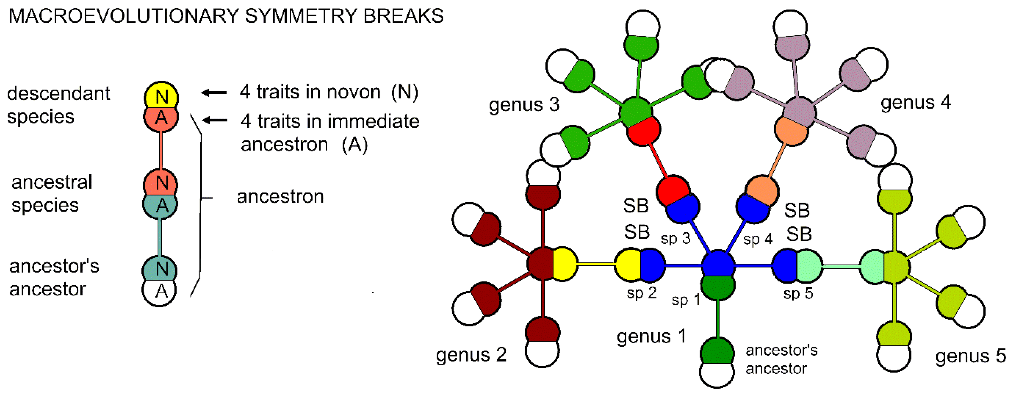
Figure 4.
Mirror parity in evolution. (Right) A series of minimally monophyletic genera concatenated serially (without major branching) is a caulon (thick line), a serial portion of a caulogram. (Left) Arrows show direction of evolution in a caulon. Each arrow is a species. The arrowhead is the novon, the set of new traits obtained by changes of old, little-used ancestron traits, and the arrow base is the immediate ancestron of traits the same of those of the novon (same color) of the ancestor. The novon and immediate ancestron mirror each other sequentially.
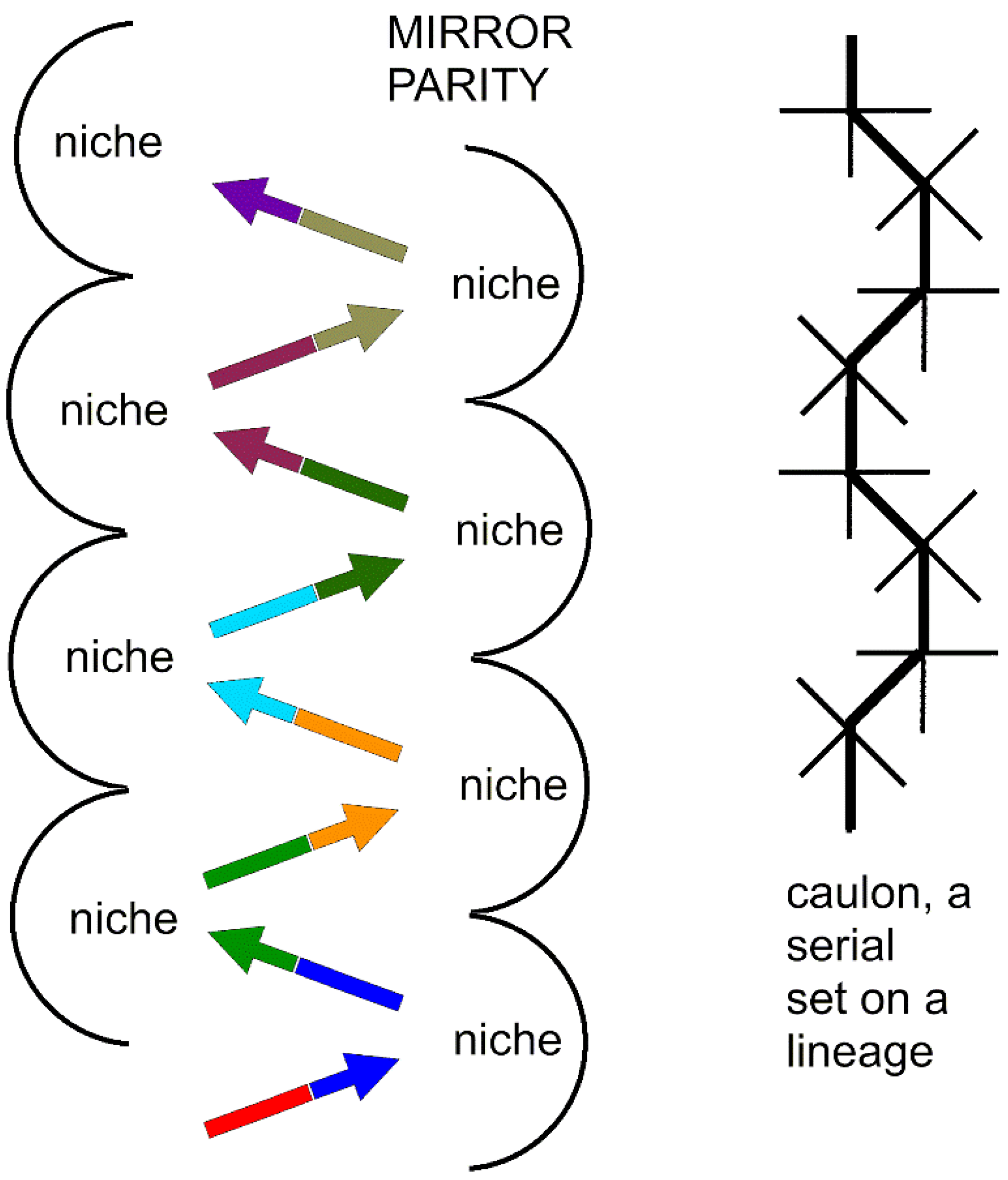
Figure 5.
Central sympatric area with peripatric “shoreline” scribble generated fractally at ln5/ln4 demonstrating potential isolation of populations that encourages genetic divergence resulting in speciation. Supplementary material HTML 120.
Figure 5.
Central sympatric area with peripatric “shoreline” scribble generated fractally at ln5/ln4 demonstrating potential isolation of populations that encourages genetic divergence resulting in speciation. Supplementary material HTML 120.
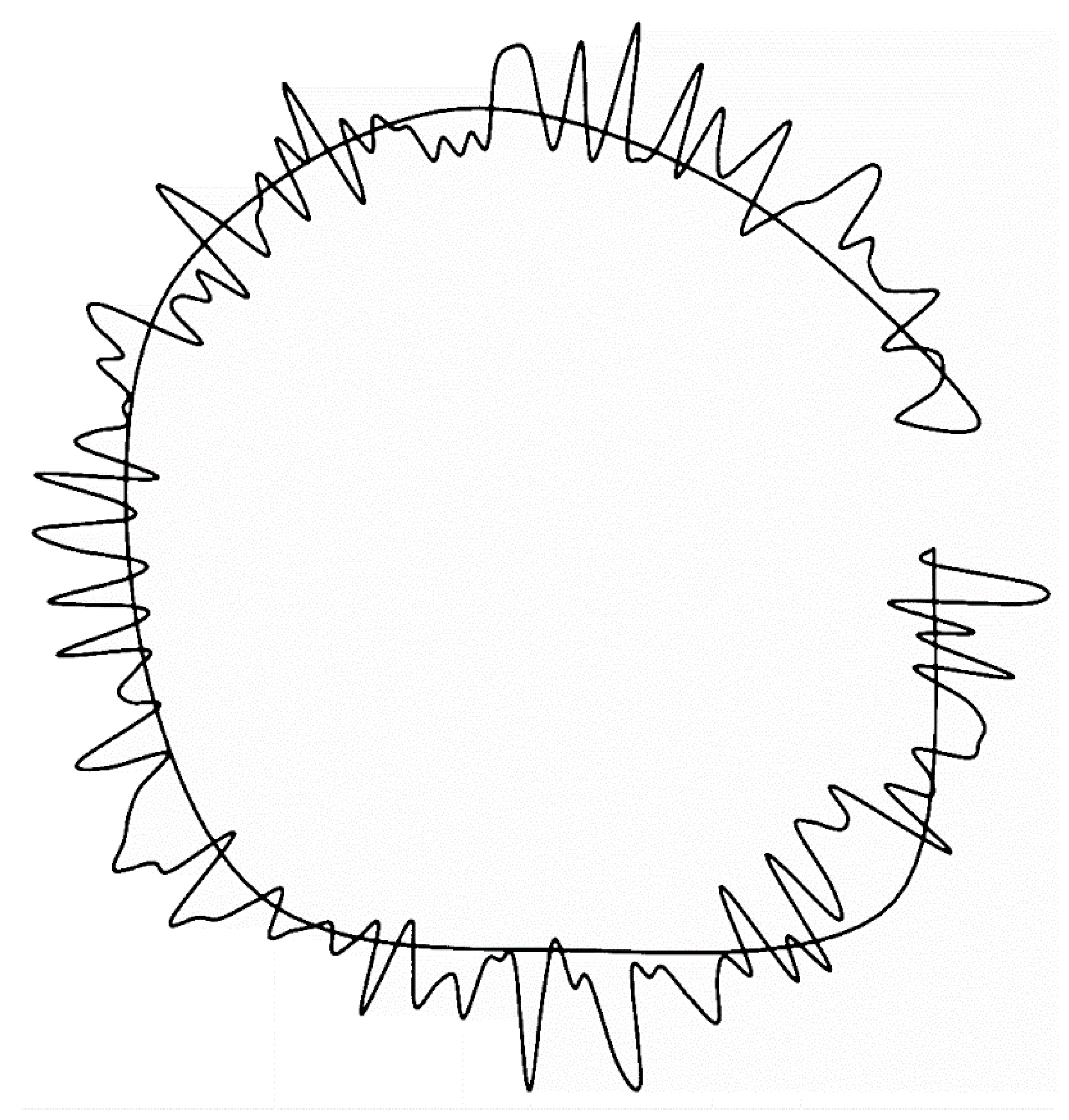
Figure 6.
Line of any length elongated 5/4, then buckled back to original length. Smoothing generates a lifelike fractal land-sea margin.
Figure 6.
Line of any length elongated 5/4, then buckled back to original length. Smoothing generates a lifelike fractal land-sea margin.
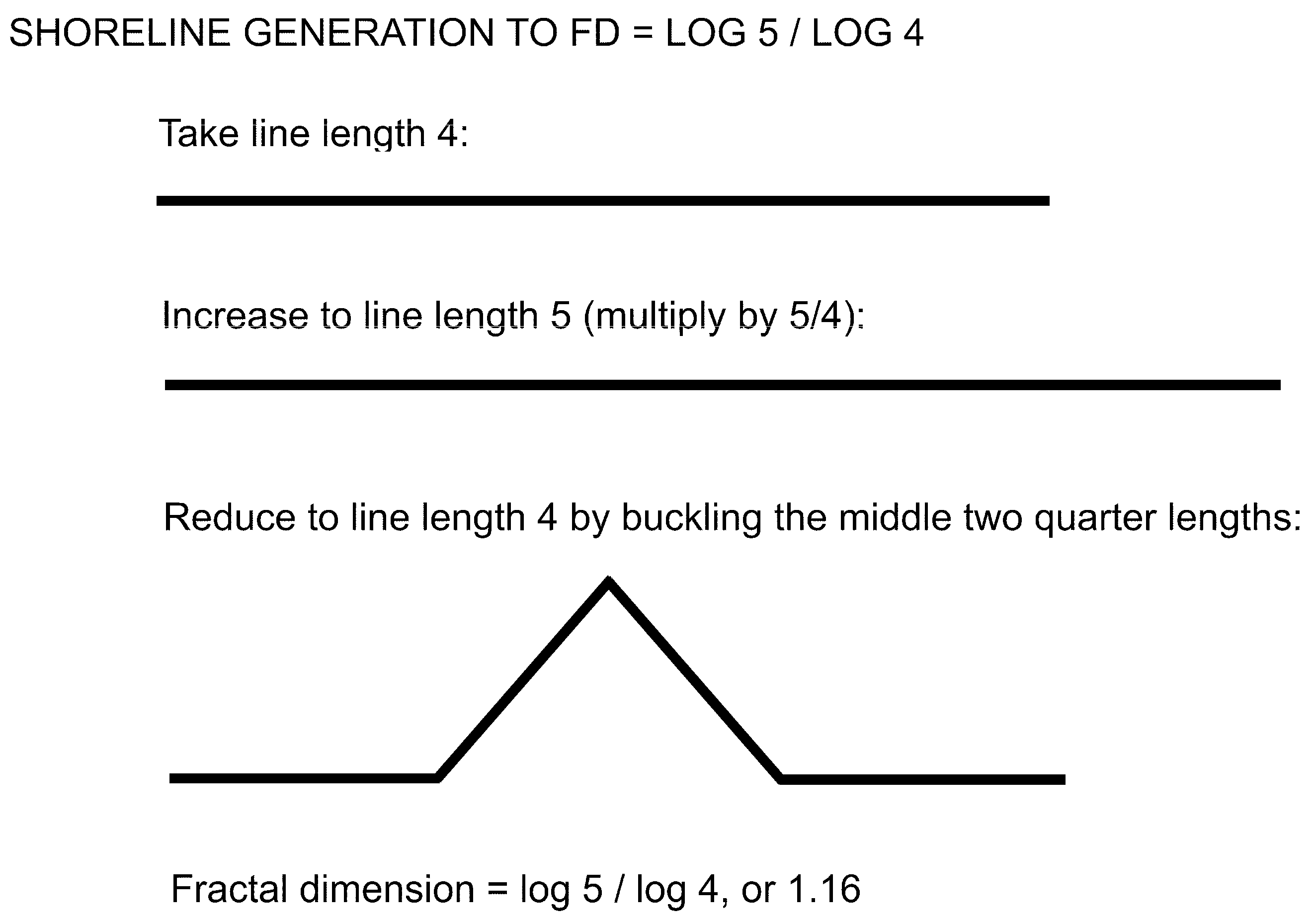
Figure 7.
Equilibrium index (y-axis) versus number of migrants per generation in island migration model (adapted from Hartl [17].
Figure 7.
Equilibrium index (y-axis) versus number of migrants per generation in island migration model (adapted from Hartl [17].
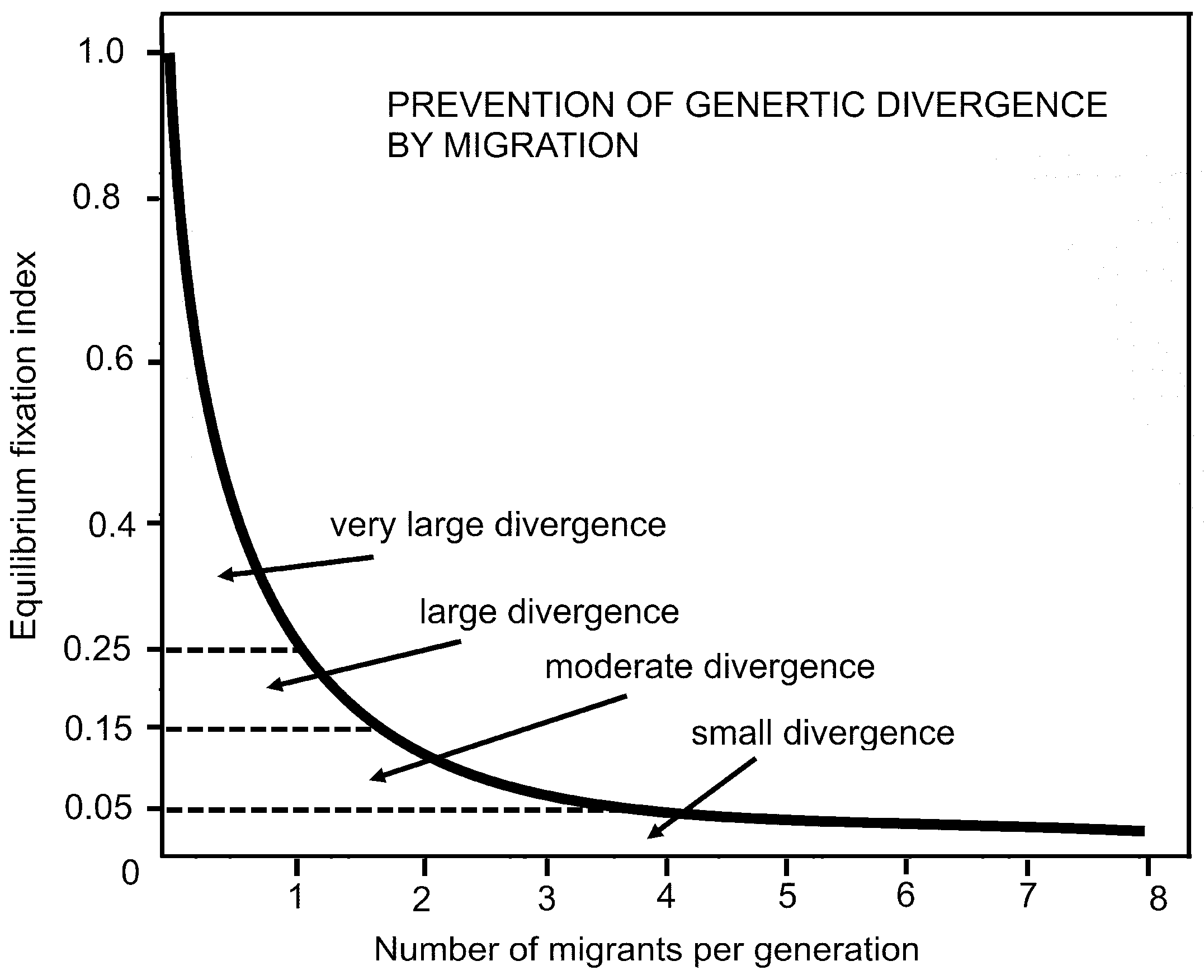
Figure 8.
Species per genus of the Pottiaceae (Bryophyta) as of 1993 from Zander [8].
Figure 8.
Species per genus of the Pottiaceae (Bryophyta) as of 1993 from Zander [8].
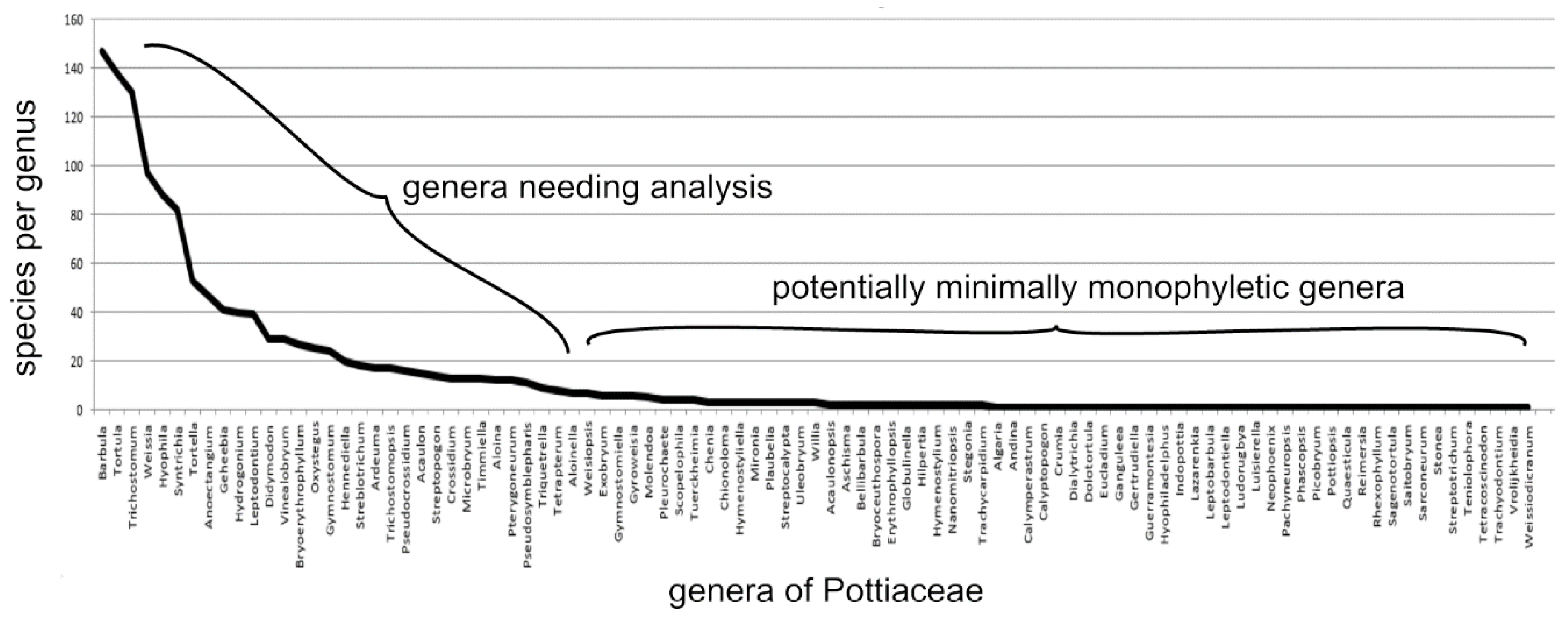
Figure 10.
The Biosphere represented as a fractal image generated with the iterated formula z = z2 + c, where z is a complex number and the complex number c is replaced with ln5/ln4 as scaling factor. Image by AI Poe Assistant.
Figure 10.
The Biosphere represented as a fractal image generated with the iterated formula z = z2 + c, where z is a complex number and the complex number c is replaced with ln5/ln4 as scaling factor. Image by AI Poe Assistant.
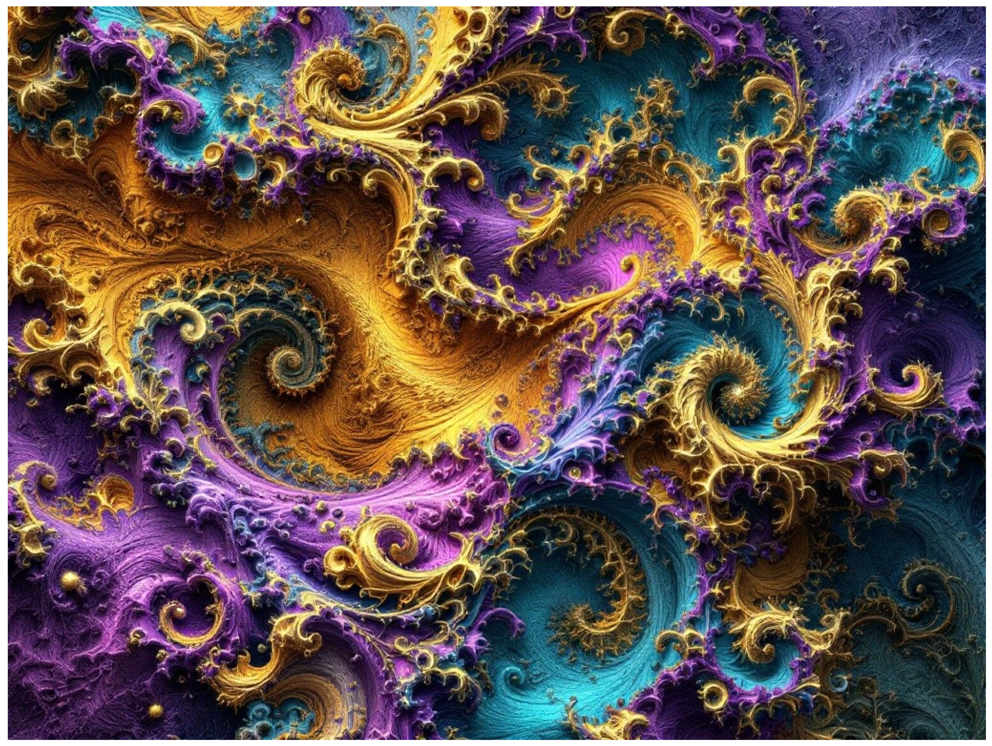
Figure 11.
Iterative function system model of the Biosphere as a hierarchically nested taxon, limited to a recursion depth of four. The ln5/ln4 paradigm is applicable at any rank because of self-similarity and scale invariance. A. Quadratic image preserving optimal 90° branching. B. Same model viewed laterally with 60° branching imposed to mimic standard evolutionary tree. Image made by AI Claude-3.5-Sonnet, see Supplementary Material HTML 150.
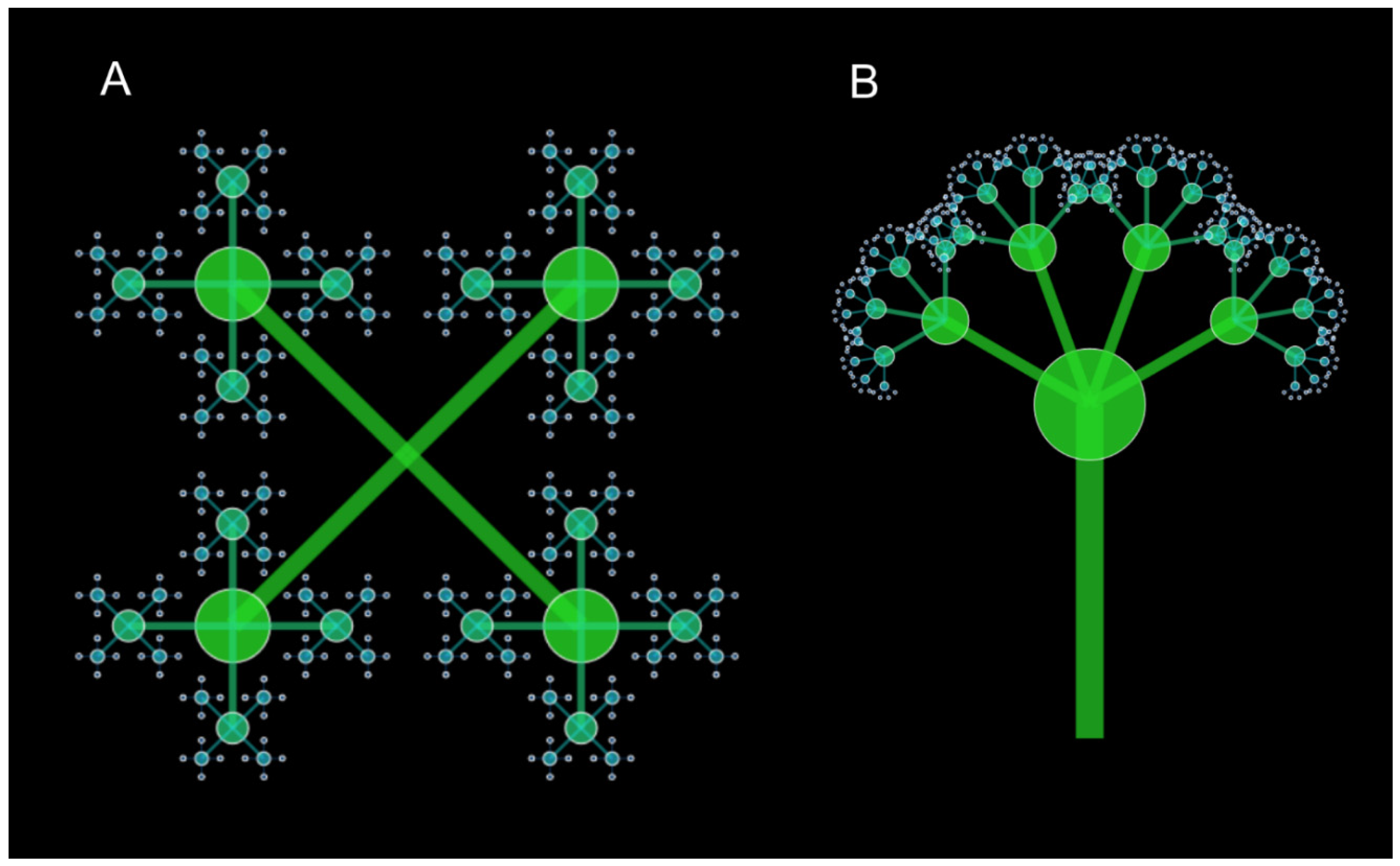
Figure 12.
Quadratic evolutionary diagram of genera and species of the Neotrichostomum complex in the West Indies. Species are not named here. The word “Genus” labels larger, unstudied groups. Numbers give size of novon (set of newly evolved traits).
Figure 12.
Quadratic evolutionary diagram of genera and species of the Neotrichostomum complex in the West Indies. Species are not named here. The word “Genus” labels larger, unstudied groups. Numbers give size of novon (set of newly evolved traits).
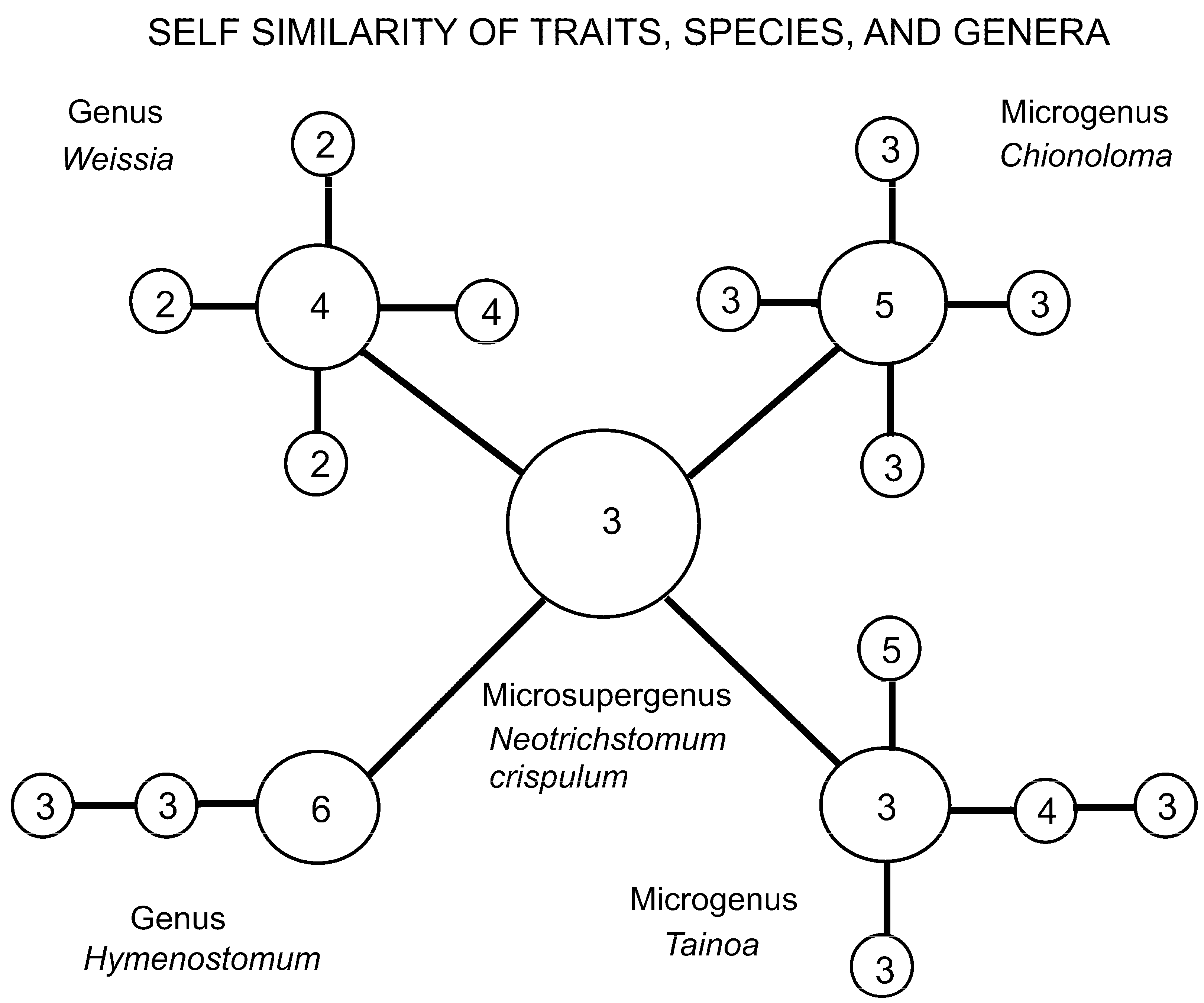
Figure 13.
Expected hollow curve for species per genus, with inset species per microgenus (minimally monophyletic group). In inset, cropped curve going up where low on x-axis is due to analysis of only speciose groups (except Streptotrichaceae), and curve absent in the trail high on x-axis (beyond 7) because of truncation by Pareto ratio inhibition of multiple descendants from one ancestral species.
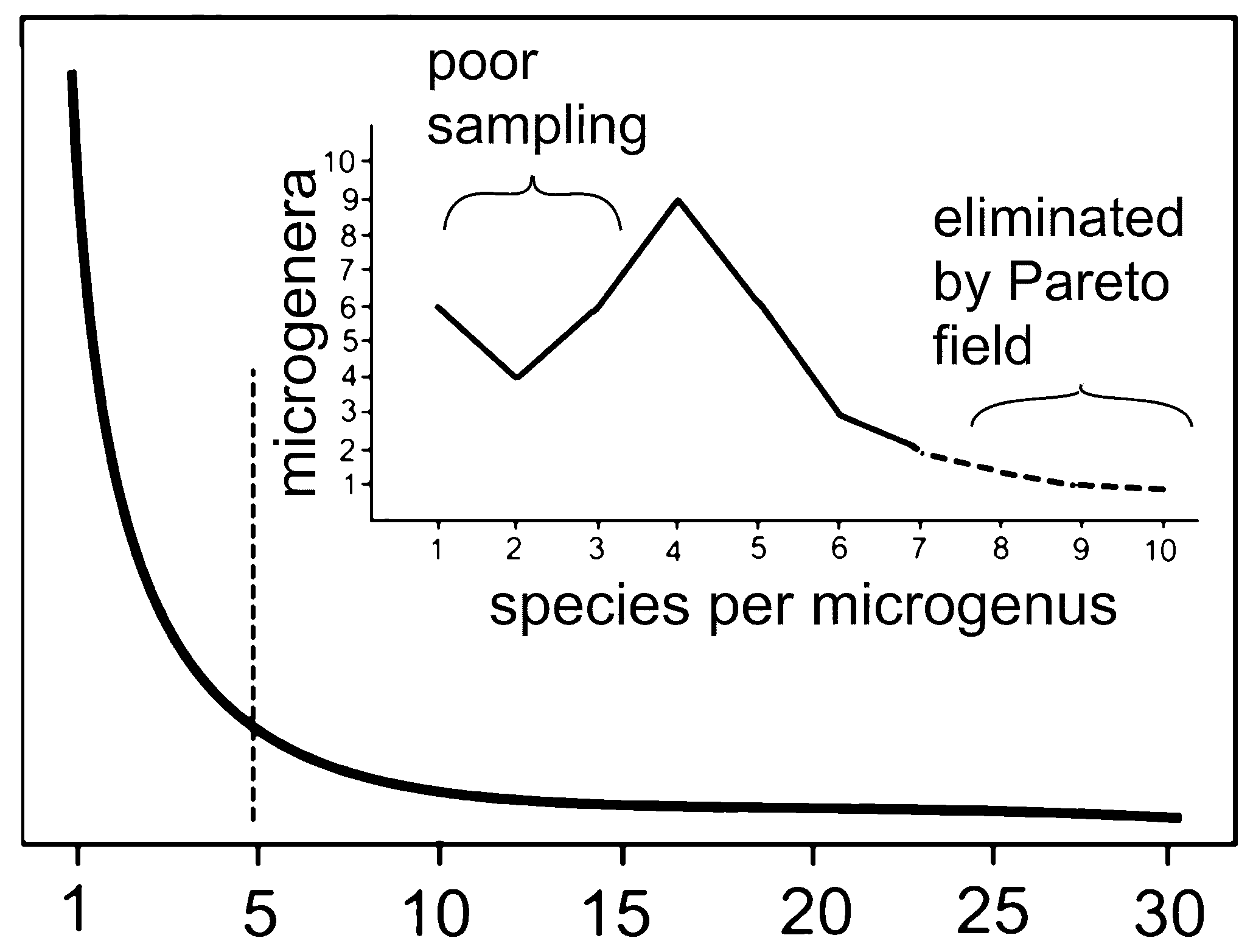
Disclaimer/Publisher’s Note: The statements, opinions and data contained in all publications are solely those of the individual author(s) and contributor(s) and not of MDPI and/or the editor(s). MDPI and/or the editor(s) disclaim responsibility for any injury to people or property resulting from any ideas, methods, instructions or products referred to in the content. |
© 2025 by the authors. Licensee MDPI, Basel, Switzerland. This article is an open access article distributed under the terms and conditions of the Creative Commons Attribution (CC BY) license (http://creativecommons.org/licenses/by/4.0/).
Copyright: This open access article is published under a Creative Commons CC BY 4.0 license, which permit the free download, distribution, and reuse, provided that the author and preprint are cited in any reuse.


