Submitted:
28 March 2025
Posted:
31 March 2025
You are already at the latest version
Abstract
Remote sensing data, particularly from Sentinel-2 satellites, offers valuable insights into surface mining activities. This study evaluates the effectiveness of Sentinel-2 imagery in detecting and monitoring sand and gravel extraction sites across five mining areas in Schleswig-Flensburg, Germany, from 2015 to 2019. Three machine learning algorithms—Random Forest (RF), Support Vector Machines (SVM), and Artificial Neural Networks (ANN)—were compared to determine the most accurate classification approach. Models were trained using three different training data scenarios to assess their performance. While RF and SVM demonstrated greater robustness than ANN, SVM outperformed the others when validated against ground truth data. Consequently, an optimized SVM-based classification model was developed and implemented in R to analyze temporal changes in the study areas over five years. The findings highlight the potential of integrating Sentinel-2 imagery with machine learning techniques for accurate and efficient monitoring of surface mining activities, offering a scalable approach for environmental management and land-use planning.
Keywords:
Remote Sensing
; open surface mining
; Sentinel-2
; Machine Learning Algorithms
; Support Vector Machines
; land use land cover
1. Introduction
Industrial minerals and raw materials, such as clay, sand, and gravel, are indispensable to modern infrastructure development, forming the backbone of construction for buildings, roads, and other critical structures [1,2]. Complex geological processes, including metamorphic and sedimentary formations and environmental conditions, govern their spatial distribution. Among these materials, sand and gravel deposits are particularly abundant and widely distributed, making them highly accessible for extraction [3]. However, the escalating global demand for these resources continues to drive both the expansion of existing mining operations and the exploration of new extraction sites, often at the cost of significant environmental and socio-economic consequences [4].
Whilst global mining exceeds 50 billion tons a year, Germany produces over 300 million tons of sand and gravel annually, highlighting the scale of extraction required to sustain industrial and urban development [1,5]. Open surface mining remains the predominant method of extraction due to its efficiency and cost-effectiveness, yet it poses substantial environmental challenges, including geomorphological alterations, habitat destruction, and long-term landscape degradation [6]These impacts necessitate robust, data-driven monitoring strategies to assess mining activities, mitigate adverse effects, and support sustainable resource governance. Advancements in remote sensing and machine learning provide critical tools for systematically tracking spatial and temporal changes in mining landscapes [7]. By leveraging these technologies, policymakers, researchers, and industry stakeholders can develop effective regulatory frameworks and management strategies to balance resource exploitation with environmental sustainability and socio-economic well-being.
Schleswig Holstein is a widespread state, with open surface mines for the extraction of raw material, particularly gravel and sand. In addition to existing mines, other zones have been categorized as potential areas for future raw material extraction [8]. Materials generated from these extractions are mainly used to meet the demands of local construction companies for building roads, residential areas, and public and private facilities [3,9]. Mining raw materials contributes to the state’s local economy by providing employment, income, and infrastructure [5]. Principles of regional planning in Schleswig Holstein concerning raw material extraction include securing the commodity on a local scale for the state while preserving its long-term use [10]. To ensure this, regular information concerning every aspect of the raw material extraction is required to make informed decisions regarding its security and management. This information from the geological survey is derived from sources such as mining, licensing, and construction companies; hence, it relies primarily on external sources for information [11]. However, spatial tools and technologies can be utilized as an additional source to fully understand the spatial development of mined areas. Collectively, these tools will facilitate regional planning by providing an internally generated assessment that can be used to complement external sources of information [11,12].
With its increasing temporal and spatial resolution, the functionality of remote sensing results in the incurring of lower costs compared to traditional methods in monitoring the changes occurring on the earth’s surface [13,14]. Satellite platforms with unique geomorphic signatures provide new possibilities for terrain mapping and analysis, which produce considerably concrete comprehension of geological processes [15,16]. Satellite remote sensing is valuable for detecting and reclaiming mining areas, providing cost-effective tools for environmental agencies [17,18]. As an advantage, it possesses the ability of multispectral imaging, which is recurring and enables continuous monitoring and facilitates predictions [19].
Through the European Space Agency (ESA) initiative, Sentinel data provides freely available higher-resolution data and shorter revisit times [20]. The advantage of having higher spatial resolution makes it more accurate in distinguishing between features, hence reducing spectral mixing [21]. Pixel analysis of satellite images remains the primary basis for producing spatially continuous land cover information and monitoring; therefore, higher pixel resolution is advantageous [21,22]. These unique qualities have resulted in more research and applications based on sentinel data.
The choice of a classification algorithm that can extrapolate and efficiently minimize the interferences from noisy satellite observations and deal with smaller training data sizes is crucial [22,23]. Machine learning techniques (e.g., Random Forests, Neural networks, and Support Vector Machines) have proven to be more efficient and accurate over the past few years than parametric algorithms like maximum likelihood [24,25]. Their efficiency is because their assumptions are not generally based on the data distribution and their provision of greater accuracies. Given that, this study focused on testing machine learning algorithms and the basis for classification for all images. Studies over the past few years that focus on land cover changes in surface mining have drawn certain conclusions [17,18]). Firstly, it has been established that it is paramount to integrate satellite images with topographic data. With the absence of light detection and ranging (LiDAR) due to limitations such as cost and accessibility, Digital Elevation Models (DEM) can be relied upon to provide basic topographical information. Secondly, it is imperative to rely on different feature measures such as feature reduction, texture extraction, filtering, and topographic parameters alongside topographic parameters to enhance the results derived from classification [17]. Optical images provide the opportunity to use different spectral indices to extract surface feature information. Lastly, comparing different machine learning algorithms is crucial to detecting the algorithm that works specifically for the studied area. Many factors account for the efficiency of a machine learning algorithm in accurately classifying satellite images; hence, it is imperative to assess, analyze, and determine which classifier performs better [26].
This study considers the above recommendations in assessing Sentinel data and its application to monitoring open surface mines to support regional planning. Through the assessment of the three different machine learning techniques (Random Forests (RF), Neural networks (NN), and Support Vector Machines (SVM), a working model based on the algorithm with the highest efficiency and accuracy is developed, which would be used to detect and analyzing surface raw material extraction sites in the region. This method is validated comprehensively and tested across the region to determine its viability, and it is applied to five different areas. Based on this model, changes occurring in the area are analyzed, including land use changes occurring over a couple of years, expansion of sites, and calculation of different metric statistics about these mining sites. Openly accessible sentinel data is the leading data employed in this study since the overall objective is to assess its contribution to regional planning and management of open surface mining of raw materials.
Therefore, the overall objective of this study is to explore and assess how Sentinel can be utilized to provide information to support and improve environmental monitoring and regional planning of open surface raw material extraction. The goal is to develop models and methods based on Sentinel 2 data, which can be used continuously across different areas and periods to analyze mining sites for open-surface raw material extraction. The following goals will be addressed:
- Examine different machine learning techniques to determine how effectively they detect, classify, and extract sand and gravel surface mines from sentinel images.
- Build a classification model set that can be used regionally for surface monitoring of mining sites.
- Use classified images from the model and perform change detection analysis of the study areas over a five-year period (2015 to 2019)
- Utilize the built model to calculate the area of mining sites for the five study areas over the five-year period.
2. Materials and Methods
2.1. Study Area
The study landscape spans across Schleswig Flensburg in the North –Eastern part of Schleswig Holstein, Germany (Figure 1). As part of the North German basin, Schleswig Holstein is located on coasts to both the North and Baltic Seas. The development of its land surface is characterized by warm periods and a series of ice age occurrences over the last two million years. As a result, some areas are covered with about up to 10 km layers of sedimentary rocks ranging from two to over two hundred million years old. This region is characterized by four seasons, with May to August being the driest; hence, all satellite images used in this study were sensed during this period. The proximity of the sea determines the climate of Schleswig Holstein, with precipitation being brought by Maritime air masses affecting all seasons, resulting in mild winters and cool summers [27]. The region has a rainfall of about 800 mm with an average mean temperature of 8°C. Schleswig-Holstein can be divided into three major physiographic regions, which are the western marshes (Marsch), the central upland belt (Geest) and the Morainic uplands (Hügelland). Deposits of salt, clay, sand and lime are located in most of the areas in Schleswig Holstein.
Five study areas undergoing mining activities were analyzed in this study since one of the goals is to assess the transferability of the method established in this study over the entire region (Figure 1). These study areas are interspersed from each other and have different properties; however, they are all characterized by agriculture fields and open surface mining sites. One or more mining excavation sites are located within these study areas, which was further analyzed. In effect, thirteen different mining sites within the five study areas were examined separately (Figure 1). Parts of mining sites below the groundwater level are filled with water, while other shallow areas are still dry. Sand and gravel are the primary raw materials extracted from these sites on a relatively large scale. Attributes of the five study areas are summarized in Table 1.
A subset of the environs around the important mining sites of focus for the five study areas was generated and named Osterby (OS), Ellund (EL), Wanderup (WA), Scuby(SC) and Klein Rheide (KR). The thirteen mining sites are also represented with OS-1, which is located in Osterby, EL-1, EL-2, EL-3 for those within Ellund, WA-1 for the site in Wanderup, SC-1, SC-2, SC-3 and SC-4 for those located in Schuby and finally KR-1, KR-2, KR-3 and KR-4 which can be found in the region of Klein Rheide.
2.2. Data
2.2.1. Sentinel Data
Sentinel 2A was obtained from the European Space Agency (ESA), and its Level 1 products were used. This image was downloaded from the Sentinels Scientific Data Hub3 (https://scihub.copernicus.eu/), an online source that offers limitless open access to the Sentinel-2 Level-1C (L1C) user products, among others. Five data tiles were used to analyze the changes these mining sites have undergone. All five study areas were located within the same tile; hence, one tile was selected for each year (Table 2). All data were chosen from May to August to minimize the effect of cloud cover. Granules were projected in the Universal Transverse Mercator (UTM)/World Geodetic System 1984 (WGS84) with a tile of 100 km by 100 km area. The data consists of 13 spectral bands, ranging from the visible to the shortwave infrared (SWIR) at 10, 20, and 60 m spatial resolutions. However, bands with a resolution of 60 m were not used in this analysis. A spatial subset of this data was executed using the SNAP version 6.0.1 tool and analyzed with a spatial extent of the five study areas.
2.2.2. Ancillary Data
Other data sources supported the optically derived information for the adequate development of a model to effectively classify and quantify excavation sites, which is imperative to achieving higher accuracies. The Digital Elevation Model from the ACE - Altimeter Corrected Elevations generated within SNAP was used to derive topographical attributes such as elevation to determine initial elevations of areas before the excavation process. The geology department of the State Agency for Agriculture, Environment and Rural Areas provided ground truth information for the various sites, including GPS points of the areas, the extent of the sites, and different attribute data and properties. Digital Orthophotos and Google Earth possessed high-resolution images over the years, which were relied upon to facilitate feature extraction.
2.3. Data Processing
2.3.1. Sentinel Data Pre-Processing
Atmospheric correction of the Sentinel-2 images was performed using the Sen2cor module version 2.3.1, a tool designed to work with Sentinel-2 images. Based on the precalculated Look Up Tables (LUTs) application with libRadtran radiative transfer routines, Sen2cor correction is made (European Space Agency, 2018). Sen2cor is designed to process S2A Level-1C Top of the Atmosphere (TOA) granules to that of Bottom of the Atmosphere (BOA) Sentinel S2A Level-2A. This processor undergoes different sub-processes to produce the final data, starting from Cloud Detection with classified scenes in the granules. Level-1C images contain water vapour content and aerosol optical thickness (AOT), which Sen2cor retrieves. The last subprocess is the conversion of the TOA to BOA. The processer also provides other processing options for the data, such as adjacency, terrain, BRDF, and cirrus corrections. The output product of Sen2cor includes images at the three spatial resolutions of the Leve1-1C, which are 10, 20 and 60 m.
This study used a stand-alone Sen2cor version 2.05.05 processor through the Windows command line to process all downloaded images. The resolution for this process was set at 10 m, with all other variables left at the default. The prerequisite to achieve this was to download the Sen2cor processor directly to the operating system.
Atmospherically corrected Level-2A images were analyzed using SNAP version 6.0.1 of the ESA. The difference in resolution of pixels for the bands required resampling, which transforms pixels into a desired resolution. To reserve the pixel values of the input images, the nearest neighbour method of resampling was utilized to transform all 20 m resolution pixels to 10 m in the product.
A subset of the image was created, and six main bands, red, Blue, Green, NIR, SWIR-1, and SWIR-2, were used for further analysis. Other bands, such as the panchromatic and thermal, were not utilized in this study due to their limited role in achieving the focus of this study and their low resolution. Images were exported as GeoTiff format files, which included all the selected bands stacked together to enable further analysis in different software programs.
2.3.2. Machine Learning Algorithms
The study accessed three classifiers: the Random Forest (RF), Support Vector Machine (SVM), and Artificial Neural Networks (ANN). RF generates predictions based on a group of predictor data by creating several Decision Trees (DTs) whose results are then aggregated. The construction of each tree is done independently using a distinctive bootstrap sample generated from the data used for training the model. RF splits its data based on a subset of training samples, which are selected randomly (Breiman, 2001). In this study for RF model tuning, parameters including a number of predictors chosen at random per node (mtry) and a number of trees (ntree) were set using a three-repetition cross-validation with ten folds from the caret package in R software.
SVM relies on training samples for classification; however, they are not sensitive to their size and hence can adapt to a limitation in training sample quality and quantity. Based on the adaptation of the Bayesian minimum-error decision rule, SVM can use iterative procedures to generate estimates to determine the probability of unknown and known classes.
The Artificial Neural Network used in this study was the feature extraction Neural Network in the caret package of the R software. Classifiers can possess one output node or more based on the different categories in which they are supposed to group samples. In this study, four classes were to be generated after classification. Precision was required to extract higher accuracies in this method and limit redundancies while the model was tuning using the caret package.
2.3.3. Training Samples and Trials for Model Development
Sentinel images in this study underwent a bands subset to extract only the bands paramount to the study: Blue, Red, Green, Near Infrared, Shortwave infrared_1 and Shortwave infrared_2. The band values were part of the training data included in the model training and building and were used to compute indices. Indices utilized for this study include the Normalized Difference Vegetation Index (NDVI), which is essential in distinguishing vegetation from other land use types. Soil indices such as Redness Index (RI), Coloration Index (CI), Brightness Index (BI), and Saturation Index (SI), as postulated by (Ray et al., n.d.) were used to extract excavation site features effectively. Table 3 highlights the method adopted for the estimation of these indices.
The resultant images of these indices applied were single virtual bands added to the initial six bands of the subset product. After the results were verified, virtual bands were saved into real bands. This process was replicated with all five indices to be derived. Additionally, the elevation was calculated in addition to the indices based on the ACE—Altimeter Corrected Elevations. At the end of the processes above, the resultant product became a subset with 12 bands, which was used for further analysis.
To effectively derive training samples for this study, external sources such as ground truth location information and orthophotos were used in addition to the satellite image used as references to select samples. The small nature of study areas required meticulous precision regarding the placement and size of polygons to avoid the model’s misclassification. ArcMap version 10.4 was the software utilized to create training samples for the classification of images. With the Editor tool, polygons were drawn over areas of interest to demarcate areas with features representing different land cover. Only four land cover classes were considered in this study: Mined area, Site water, Vegetation and Fields. Even though the analysis of the mined site is the emphasis of this study, these other classes were distinguished to determine the state in which present and abandoned sites have returned.
Polygons for each land cover class were collected for each study area and all five respective dates to increase accuracy efficiency. This effectively captures all the different spectral signatures for the class within the region. The decision to use polygon shapefiles enables easy editing in ArcMap when regions demarcated are inaccurate. Hence, classes can be modified to obtain the best results. These polygons contain different pixels with different values and are the basis for the classification. To test the models developed, a different data set was gathered for validation based on the ground truth information discussed above.
2.3. Model Set-Ups and Calibration
2.3.1. Model Set-Up of Machine Learning Classifiers
Initially, the selected variables that would serve as inputs were selected band registrations of the Sentinel optical imagery, namely the Blue, Red, Green, Near Infrared, Shortwave infrared_1, and Shortwave infrared_2, in addition to the five indices calculated in section 2.2.3. Secondly, topographical information such as elevation was also intended to be utilized in the model building. The three models were all fitted with the first set of data, which were twelve in total and tested. The aim of this was to test for the influence each variable had on the entire model and its importance to the classification. Different combinations of variables were tested in different model set-ups. The six bands were fitted with the elevation data, indices, and classes, which were then fitted without the elevation but with classes. The model with the four 10 m bands was also fitted alongside the elevation and classes. Finally, the four bands with the classes without elevation were also fitted. This fitting and testing were done for all three classifiers: RF, SVM, and ANN.
Three model scenarios were analyzed after deriving the best factor for observation and variable with the uttermost importance. In scenario one, the model was independently fitted in the three classifiers for all the study areas for all five years, with training data derived explicitly from their respective regions. The second scenario was characterized by a model built based on the yearly data derived from all the study areas in that year and collectively used to develop a model to classify them individually. The accuracy of these scenarios was computed and compared to derive the best model classifier, which would be used for further data analysis. In the last scenario, all the input data gathered over the five years were merged, tuned, resampled and trimmed to build the model based on the classifier selected and used to classify the images of study areas for all years.
2.3.2. Calibration and Validation of RF, SVM, and ANN Classifiers
Different data sources were required to effectively develop, calibrate, and validate the three models for classification, including optical-based land use information, location and extent data from the geological department, elevation resources, high-resolution images and Google Maps services. The same methodology was applied to all three domains in terms of calibration, validations, and prediction. The e1071 package in the R software was employed to tune the model for the machine learning Algorithm employed.
The assessment of the three models was conducted internally to derive the combinations of optimal parameters, respectively, using the 10-fold cross-validation of the training set. This method divides the training sets randomly into 10 different subsets of approximately the same size. Consequently, nine out of ten subsets would be used as training data for the models, and the remaining data set would be used as testing data. This action is repeated three times so that all the datasets have been tested against each other. A seed was set to ensure the same samples were utilized for all the models. With random stratified sampling, the training set was divided to fit and validate all the models. The employment of the grid search method enabled the selection of the parameters that best fit the model. Overall accuracies of all the models were derived from the average values after all the ten processes that have been run.
2.3.3. Accuracy Assessment
The RF, SVM, and ANN were used to predict and classify mining sites, and they were assessed using the entire training sample gathered for cross-validation. A summary of the internal validation was computed, which provides performance statistics focusing on the Accuracy and Kappa co-efficient of the three models. The results derived from the summary show Accuracy and Kappa in terms of their mean, median, minimum, maximum, 1st quarter, and 3rd quarter. The R software was used to compute the results of the repeated cross-validation to test the accuracy of all the classifiers. The classifier with the highest accuracy was tuned and optimized to classify images.
The assessment of the strength of the model outside the training sample is performed with different validation data acquired independently of the training sample. External sources like digital orthophotos and Google EarthPhotos to obtain yearly data for the past five years. Boundaries and parcels of land where mining activity was being undertaken were also obtained from the LLUR and GPS point location data. Previous field observations and yearly land use data would be the optimum mode to extract validation data; however, its unavailability resulted in the reliance on the above data. Based on this data, polygons and points were generated and used to extract pixels which would be utilized for validation purposes. Yearly validation data was generated for the different locations and used as input to test the accuracy of the given models. In effect, validation data was generated to test the various scenarios of analysis based on training data. These validation samples are set aside for the external accuracy assessment of models.
The validation data for all the study areas was used to compute a Confusion matrix, which provided different analytical and descriptive measures and effectively summarised classification accuracy. The Confusion Matrix or error matrix is based on and effective for classification, where each pixel can only be assigned to a single class. In effect, the accuracy depends on whether the model can effectively correctly group pixels into their assigned single class. Consequently, the calculation is done by analyzing the area of the portion classified correctly in relation to the number of pixels misclassified. The hypothesis is that each pixel signifies only one class, resulting in the binary encoding scheme, one-out-of- c classes, since the output data must reflect the reference data (Bishop, 1995). Since pixels are assigned one in their target class and zero in all other classes, it results in a mutually exclusive dataset.
2.4. Classification of Images
The SVM model was optimized in different steps to classify images, which would be used for change detection in this study. The initial step was to determine the correct value of C, which produces the highest accuracy, and the correct raster cells, which served as training points extracted from the images to be utilized. This is done considering the available computational resources and the average range of errors.
The next step involved quantifying each predictor’s role in the estimation of classification. Calculations derived from the SVM algorithm were analyzed to identify which variables played a more significant role in the classification. Unlike other studies, variable importance was not manually scaled but left to the interpretation of the model in order not to influence how the importance test is conducted. Working with twelve (12) initial predictors required fine-tuning the model and testing the viability of these predictors. To achieve this, predictors were eliminated one by one from the entire data set to observe the changes had on accuracy. The goal for this was to determine the best predictors to be utilized based on results with the results from the confusion matrix.
Several tests and tuning were conducted to produce the highest accuracy and reduce computation time and the memory needed to run the model. All values were left to default in the initial run, and the different performances were analyzed to determine the best C value for the final model. This test was performed on the study area Schuby (SC) for 2015.
2.5. Post-Classification Change Detection and Area Calculations
A post-classification change detection technique was adopted for this study. The land cover changes yearly were first calculated for the already classified images with the cross-tabulation method from (2015-2016), (2016-2017), (2017-2018), and (2018-2019). This method produces information on both the quantitative and qualitative trends of changes. The changes between these dates can be visualized based on a simple technique. A change matrix was computed using QGIS 3.4.
Estimation of the area of the mines undergoing mining over the five-year study period was performed based on the classified images derived. Mined areas of all 25 images were extracted, and the areal extent was estimated. Ground truth information, which provides the borders of mines, was used to crop the classified images to derive only areas of interest. Before that, all other pixels were removed using the R software, and only pixels representing mined areas were left for further analysis. Area values were calculated for all the mined sites and the water on the mining site to determine whether the water has also increased. Figure 2 illustrates the overall workflow of the methodology adopted for pre-processing images, the model development process, statistical analysis, and the change analysis.
3. Results
3.1. Accuracy Performance and Visual Assessment of Models Specific to Study Areas
3.1.1. Accuracy Performance of Models
Table 4 presents the accuracy assessment results of the first scenario (the study area dependent model), which uses data specific to that area for a particular year. To assess this, 25 models were built for each classifier, resulting in 15 models per year and three (RF, SVM, ANN) different models per study area for each year. Kappa co-efficient and Overall Accuracy for the three classifiers were computed for the study areas of Osterby (OS), Ellund (EL), Wanderup (WA), Schuby (SC) and Klein Rheide (KR) yearly from 2015 to 2019.
For 2015, the SVM and ANN models developed to classify OS possessed the highest accuracy (99.94%) and Kappa (99.91%) and had the highest values among all the sites for that year. The lowest accuracy for that year was also recorded for SVM, with 99.01% and a Kappa of 98.52%. RF proved to have the highest accuracy for three of the study areas, EL, WA, and KR, while SVM recorded the highest accuracy for two OS and SC. Models developed to classify 2016 images of study areas all possessed accuracies ranging from 96-99%. RF recorded the highest accuracy (99.84%) for all the models that year, while ANN and SVM recorded the lowest of 97.81%. RF model developed for all the study areas proved to have the highest accuracy compared to SVM and ANN, while ANN proved the second highest for four study areas (EL, WA, SC, KR). RF model for classifying the study area SC proved to have the highest accuracy (99.97%) out of all the models for 2017.
The lowest was, however recorded for the SVM model of OS with 98.28%. RF model once again demonstrated the highest accuracy for all the study areas, with ANN following in close second for four of the study regions. With an accuracy value of 99.97%, the RF model for the KR study area was the highest for 2018. Ironically, this year’s lowest accuracy (84.65%) recorded was also that of the RF model, but it was for the OS study area instead. Evidently, RF did not have the highest accuracy for all the study areas this time; however, it had four (EL, WA, SC, KR) out of the five. ANN model had the highest accuracy in the OS study area and the second highest in three other areas. The accuracy value of 99.73% was the highest for 2019, which belonged to the RF model for the classification of the WA study area. Once again, the SVM model for OS had the lowest accuracy at 90.87%, and the RF models had the highest accuracy in all the study areas.
Generally, it can be deduced that RF models performed better and are more robust regarding the training data used for developing the models. Of the 25 RF models built, 20 proved to have the highest accuracies compared to their counterparts. Despite having the highest accuracy in only two areas, ANN models proved to have comparatively higher accuracies than SVM for 16 of its models. SVM performed the least compared to the other classifiers despite having the highest accuracy for two areas. Conclusively, for this study, it can be inferred that when it comes to models for the classification of a specific location, which are trained with data from only that area, RF models usually have the highest accuracy based on internal validation.
3.1.2. Visual Assessment of Classification Results
Seventy-five classification maps were derived from the three machine-learning classifiers. For the visual analysis, however, the classification images for 2015 are used to show the disparities between classifiers, as shown in Figure 3. The differences in the type of error are visualized with different rectangle colours in the images.
One of the visually eligible errors of commission can be identified in the misclassification of other classes for water, which is represented by the black rectangles. Evidence of this can be seen in all the different SVM-based classified images. A misclassification between vegetation and fields is a typical error in the ANN-based classification presented with red rectangles in Figure 3. Disparities between RF and SVM classifications are minimal compared to the ANN classifications, showing slight visual differences. The blue rectangles show the misclassification of other classes for the mined area, which is typical of the ANN-based classification. One of the most visible errors is the classification of roads as water or mined areas instead of fields; the white rectangle shows an example of this. Visual analysis of the images matches the accuracy results generated using the internal statistics compared to the actual data.
3.2. Accuracy Performance of Models Specific to Years
3.2.1. Internal Validation
As mentioned earlier, for scenario two, models for the three classifiers were built for each year of study, resulting in five models per classifier. Investigation into the three model’s performance was assessed dependent on both internal accuracy statistics generated and validation samples independent of the training samples. The comparison between the different Accuracies and Kappa derived from the internal statistics of the three models was used to achieve this assessment. The results of the comparison are presented in Table 5. The Accuracy ranged from 98 to 99% for the RF, between 97 and 99% for SVM and ANN had 96% to 99%. Kappa Co-efficient also ranged from 98 to 99% for RF, SVM ranged from 95 to 99%, and ANN ranged from 93 to 99%. The highest accuracy and Kappa were recorded for the RF model for 2017 at 99.9% and 99.83%, respectively. Lowest accuracy and Kappa were also recorded for the ANN model for 2019, with 96.32% and 93.86%, respectively. The performance of the RF model was its highest for 2016 and its lowest in 2018. All accuracies for the RF model were above 99%, except for 2018, which was 98%. SVM and ANN models recorded their highest accuracies for 2015, while their lowest values were for 2019. Generally, the models for classifying 2019 images had lower accuracies than other years. ANN models consistently had the weakest accuracies and Kappa values for all the years. In contrast, all the models with RF and SVM classifiers had the highest accuracies. They hence tested as the models with the best performance through internal assessment based on cross-validation.
3.2.2. External Validation
Validation was done externally using data gathered separately from the training data from different areas. Validation data was collected specific to the various study areas and their different land use types; hence, data was specific to all five study areas for all the different years. The accuracy, Kappa, and Specificity for the class mined area generated were also calculated for all the sites. Results from the confusion matrix computed between the predictions based on the model developed and validation data specific to the site were analyzed.
Results show that for 2015, three areas (WA, SC, KR) had perfect accuracies, Kappa and Specificity for all three models, hence 100%. The other two areas (OS and EL) saw the SVM model with the highest accuracy of 100% and 99.92%, respectively. All the specificity values for the class “mined area” of the SVM model for all study areas were 100%, suggesting no false positives in their predictions. The ANN model recorded the highest accuracy for four areas out of the five in 2016, while the SVM model recorded the highest in the remaining. The area KR had the lowest accuracy recorded for that year, with 77.1%, which was an ANN model. The SVM model for the year 2017 recorded the highest accuracy for four of the study areas compared to its counterparts. Once again, all the specificity values of the SVM model for all areas were a perfect score (100%). The SVM model for this year performed better than the RF model for all the other years with comparatively higher accuracies, Kappa and Specificity. The 2018 ANN model produced the highest accuracies for three study regions, while the RF model and SVM had the highest for one study area each. An accuracy of 100% was achieved for the 2019 RF model for the KR study area, even though the model was only the highest in accuracy for one other area. The SVM model proved to possess the highest accuracy for three of the areas.
It is clear which classifier performed better compared to actual validation data outside the training data. Granted, the SVM models performed better than the ANN and RF models; however, the results of the internal validation were not as homogenous. Figure 4 shows the variations of model accuracies for the three classifiers yearly for the five-year period when external validations were conducted. The different ranges of accuracies from the various models can also be analyzed.
3.3. Accuracy Performance of Overall Model
3.3.1. Internal Accuracy Statistics
In scenario three, all the training data gathered over the five years for all study areas were combined to train one model per classifier. Internal accuracy statistics were computed for each model, which produced accuracy and kappa results based on the cross-validation method were used for this assessment (Table 6). The RF model had the highest accuracy (99%) and Kappa, while the ANN model recorded the least accuracy with 96%.
3.3.2. External Accuracy
Model performance was assessed based on the validation data gathered from the areas of study for each year. Here, the accuracy, Kappa, Specificity, and the matric table were calculated and used to compare the different models. Table 7 shows the class mined area’s accuracy, Kappa, and Specificity. The RF model recorded 100% as its highest accuracy and 63% as its lowest accuracy. On the other hand, the SVM model has its highest accuracy of 100% as well but has a relatively higher lowest accuracy of 77%. The least high accuracy was recorded for the ANN model, which was 98%, and the lowest accuracy was 63%.
The accuracy results for the study area images of 2015 saw the SVM model having the highest accuracy for four out of the five study areas with an accuracy of 100%, while the RF model had the highest for one study area with 98.7%. SVM performed better in 2016 as well. However, RF had the highest accuracy for two of the study areas that year. This year, the ANN model consistently remained with the lowest accuracy and Kappa. The SVM model performed the best in classifying the 2017 images as well. Its Specificity was 100 % for all the study areas while having the highest accuracy for four out of the rest. The accuracy and Kappa of SVM were the highest for four study areas of 2018 compared to the ANN and RF models, and its Specificity was recorded at 100% for three. The result for 2019 is the only one recorded where the SVM model was the highest for all study areas.
A total of 20 out of the 25 images classified assessed recorded the highest accuracy performance for the SVM model. A percentage of 92 of all images classified based on the SVM model recorded accuracies above 95%. Regarding the classification based on RF, 72% of the images classified recorded accuracies above 95%, while the ANN model has only 28% of its images achieving this. A specificity of 100% was also recorded for the 72% of images classified for the class mined area by the SVM model.
The confusion Matrix results (Figure 5) for the three models for the classification of the 2019 images were also analyzed to assess the errors in classifications for all the models. All the images classified with the ANN model misclassified the site water for other land cover types (Figure 7). This error is not noticeable when only the accuracy and kappa values are considered; hence, it is paramount to analyze the different land cover classes to determine which classes were misclassified.
The specificity values, even though they summarise the false classification that a model has produced, do not show the exact misclassification errors. However, the low specificity values for the ANN model drew the attention of further analysis with values as low as 0.66. Further analysis of the confusion Matrix revealed the inability of the ANN model to effectively classify the class site water for all the images from 2015 to 2019. Classification error disparities between the RF and SVM were minute and similar. All the models had noticeable misclassification errors in the classification of vegetation as fields (Figure 5)
3.4. Classification Results and Performance with Support Vector Machine Model
3.4.1. External Accuracy
The SVM model performed better based on external validation and, in effect, was selected as the classifier for change detection analysis. One general model set was tuned and developed based on all the data gathered in the study landscape. Table 8 illustrates the overall accuracies and F1 scores of all the classifications generated based on external validation with data outside the training data set. The overall accuracy of Osterby (OS), Ellund (EL), Wanderup (WA), Schuby (SC) and Klein Rheide (KR) for the year 2019 is around 98.7%, 97.9%, 99.9%, 97.8% and 100% respectively (Table 8). The F1 score for all sites is higher than 90% for all the study areas, which indicates a model performance which is robust.
3.4.2. Variable Influence on Classification
The highest accuracy in the classification of this model is achieved using all the variables mentioned in section 2.3.2. Different combinations of the parameters showed that combining all parameters as a single unit generated the highest accuracy and hence was implemented in this research. Using only the three true colours and NIR yielded the least accuracy; however, it increased by 0.3% when SWIR-1 was added to the combination. An addition of SWIR-2 to the combination saw a sharp and highest rise by 1% an accuracy of 98.05%. The addition of NDVI, BI and Elevation provided an increased accuracy of up to 98.4%. Table 9 shows the average transition in accuracy based on the different combinations analyzed.
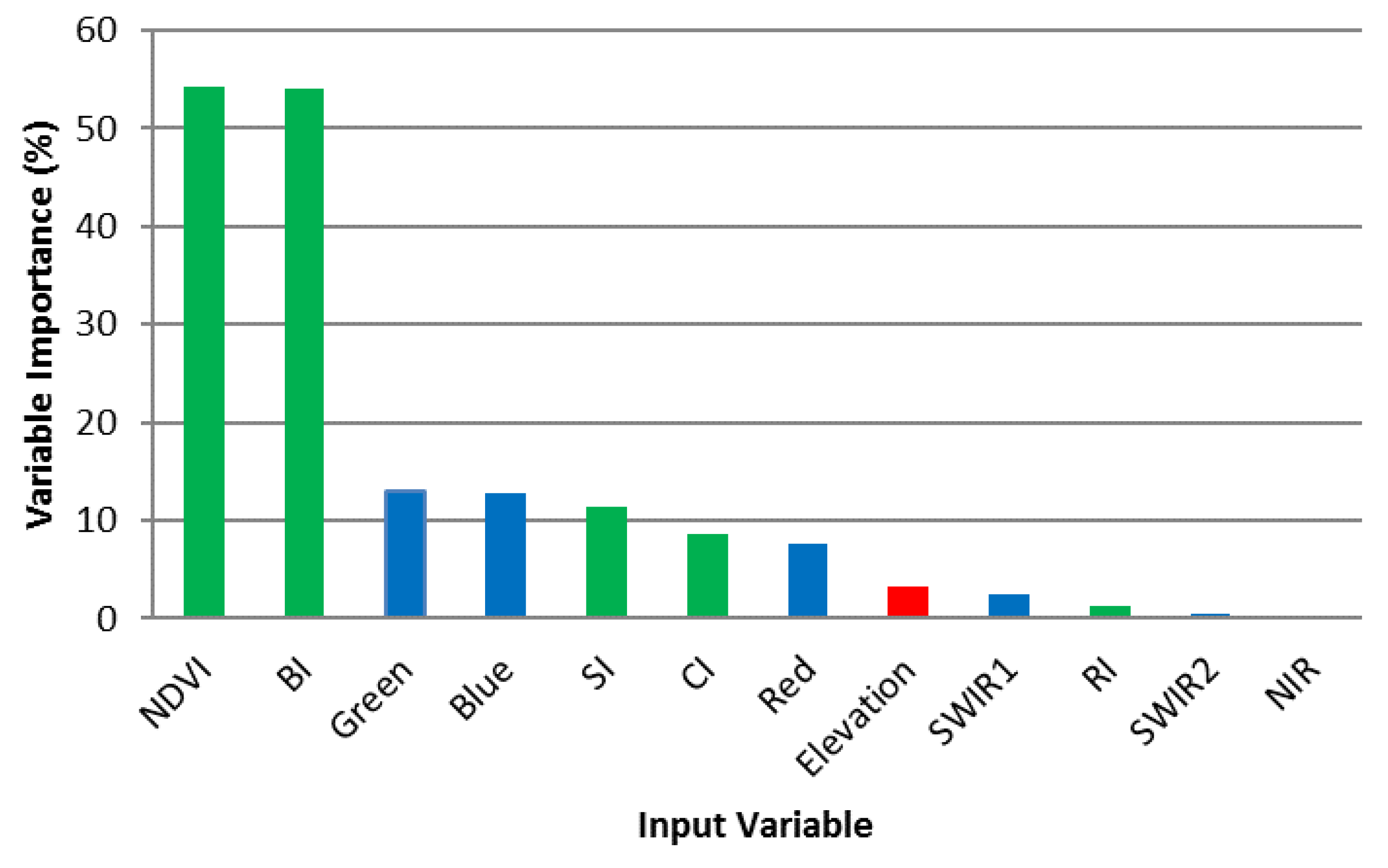
The independent parameter’s contribution to the model can be determined by the ranking of the variable importance which is derived from the model. Different weights were applied to the parameters to determine which variable played an important role in the classification of images. General importance is illustrated in Figure 6 of the variables used for building the model. It is clearly established that the indices possessed the highest importance, especially the NDVI and BI. The green and blue were of the highest importance among the six bands, while NIR recorded the least importance. Other less important variables include SWIR-2, RI and SWIR-1.
Figure 6.
Graph showing the importance in percentage of the different input variables for training the SVM mode.
Figure 6.
Graph showing the importance in percentage of the different input variables for training the SVM mode.
3.5. Spatial and Temporal Assessment of Land Use Changes from 2015 to 2019
3.5.1. Changes in Mined Areas
Table 13 summarises the area extent of the different land cover classes in square kilometres and the percentage area it covers for the five different time periods. Table 14 also summarises the changes which have occurred from 2015 to 2016, 2016 to 2017, 2017 to 2018 and 2018 to 2019. Significant changes have been experienced over the five years for all the different land cover types, including mined areas, water, vegetation and fields in all the study areas, and these tables and figures highlight this.
Mined area land cover basically consists of portions of the study area surface which have been mined or are undergoing mining. This class experienced a gradual increase in area and rate of changes over time due to continuous anthropogenic excavation activities in these areas. The total area of the mined area land cover is estimated at 0.06 km2 in 2015, 0.09 km2 in 2017 and 0.1 km2 in 2019, which equals 1.39%, 2.08% and 2.31%, respectively, for Osterby (Figure 7). Mined areas significantly increased at a positive rate of 0.04 km in this area which represents 1% (Table 10) from 2015- 2019. Ellund had the least increase in the size of mined areas, with only a 0.15% increase from 2015 to 2019, representing an area increase of 0.003 km2. This area experienced a decrease from 2015-2018 (0.36-0.34 km2) but saw a quick increase to 0.38 km2 in 2019 (Table 10)
Another area which experienced minimal changes in the mined area, though higher than Ellund, is Wanderup, with an increase of 0.25% by the year 2019 and an area kilometre of 0.05 km2. Area extent for 2015 was 0.29 km2 which increased to 0.31 km2 in 2016, decreased again to 0.3 km2 in 2017, and finally increased to 0.34 in 2019 (Table 10). Schuby’s mined area experienced a constant increase over the years from 2015 to 2019 (0.24-0.31 km2) but had the largest from 0.26 km2 in 2018 to 0.31 km2 in 2019. In effect, there was an increase of 1.23% over the years in the mined area class. Klein Rheide recorded 0.7, 0.81, 0.82, 0.87 and 0.9 km2 for 2015, 2016, 2017, 2018 and 2019, respectively, which represent 4.49%, 5.19%, 5.26%, 5.57% and 5.77%. The highest percentage increase can be observed in this area with 1.28%.
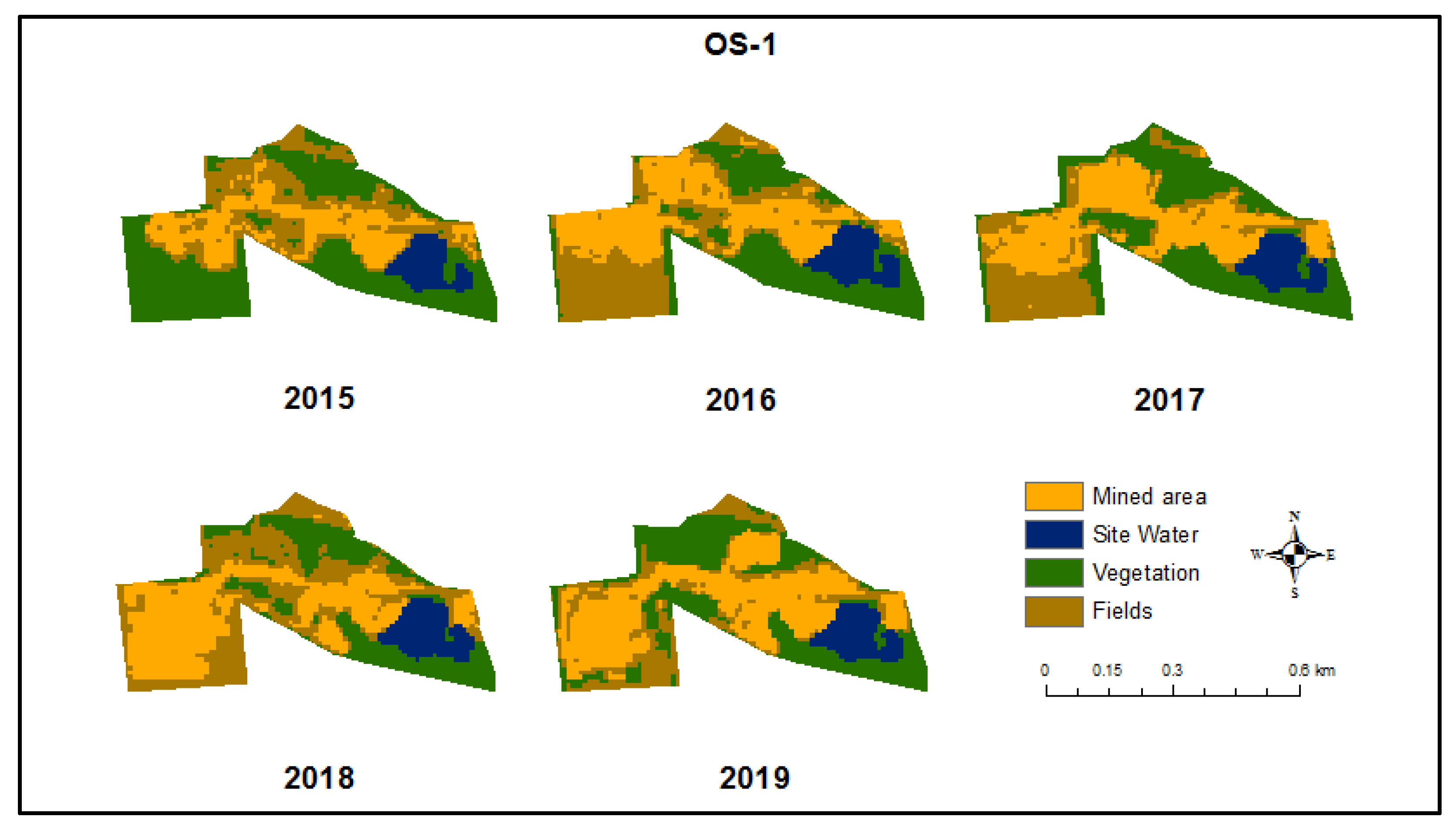
Figure 7.
Images showing the mining site (OS-1) in Osterby and its land cover changes over from 2015 to 2019.
Figure 7.
Images showing the mining site (OS-1) in Osterby and its land cover changes over from 2015 to 2019.
3.5.2. Changes in Site Water
The water bodies constitute open surface water mostly found in areas undergoing mining activities in various parts of all the study areas. Areal coverage of water for Osterby was constant across all the years, with only a slight increase of 0.03 km in 2015, while all other years recorded 0.02 km2. Waterbodies represented about 0.46% of the entire study area. The water class in Ellund, on the other hand, experienced a decrease from 2015 to 2017 with 0.17 km2 to 0.13 km2. An increase to 0.16 km2 was recorded in 2018, which was succeeded by a reduction to 0.13 km2 again in 2019 (Figure 8). Water in this study area has an area increase slightly above 1% for all the years. Wanderup is one of the areas that clearly highlight the extent of site water. Though constant, it is the largest site water among all the study areas with the lowest area being 0.62 km2. It possesses the same trend as Ellund, with a decrease in the area till 2017 and an increase in 2018, which decreases again in 2019. The water class in Schuby has a total of 0.02 km2 of increase from 0.15 km2 (2015) to 0.17 km2 (2019). A dip was, however, experienced in 2016 to 0.14 km2. From 2015 to 2016, water in Kleine Rheide experienced a sharp decrease from 0.23 km2 to 0.18 km2, which remained constant until 2018, when it rose to 22 km2. A 0.33% decrease in water was recorded for Kleine Rheide (Figure 8).
4. Discussion
4.1. Methods Employed for Classification of Sentinel Data
4.1.1. Application of Sentinel Data
Sentinel data and tools for its processing enable easy manipulation, analysis, and derivation of information for monitoring [28]. Sentinel-2 imagery provides the ability to map land cover at a finer scale and with a higher fragmentation degree to easily distinguish between features. The fine resolution, both spatially and spectrally, facilitates improved image analysis and mapping of land cover on a local scale [29]. Given that, by selecting certain combinations of bands, diverse spectral properties can be emphasized or downplayed, which allows for easy extraction of features of interest [30]. A high level of detail was obtained when compared to orthophotos, field validation, and ground truth data, which serves as a viable solution for the evaluation of hazards, protected areas, spatial planning, and environmental monitoring [31].
Pixel image analysis of satellite images remains the main basis for producing spatially continuous land cover information and monitoring ([32]). In effect, as input data for classification, the Sentinel provides superiority due to its higher pixel resolution and reduction in pixel mixing. [19] were not able to classify all classes in surface mining and reclamation because of the low spatial and spectral resolution of Landsat. It reaffirms the claim by [33] that rich spectral and pixel information provides helpful details in distinguishing between land cover types.
4.1.2. Effectiveness of the Support Vector Machines (SVM) Model
Conclusive results from this study show SVM had the highest classification accuracies when compared to ground truth data followed by RF and ANN using both all the training data or a subset of the training data. The RF was a close second and had high accuracies with internal statistics; however, it could not excel when compared to the validation data. Comparison of different machine learning techniques, as shown in earlier studies, have had similar results [34]. Studies of surface mining surfaces determined SVM to have greater accuracies in the classification of mines and reclamation compared to RF [17,18]. Regularly, RF and SVM algorithms outperform ANN and have shown similar superior accuracy results [35]. The SVM algorithm showed more sensitivity to the training inputs compared and could be manipulated to increase accuracy.
SVM has the unique property of having the ability to maximize class margins through the separation of different land cover with a decision surface, hence reducing the overfitting of spectral responses [36,37,38]. As a non-parametric type of algorithm for classification, it possesses the quality of producing positive results amidst noisy and limited data, provided it possesses a spectral variability which has a wide range among the different land cover types [38]. Results derived from this study proved SVM is more robust in the extraction of mining sites compared to RF and ANN. [30], also iterated this in their research, which showed SVM returning higher accuracies and better classification results compared to neural networks.
Similar conclusions were drawn from the mapping of surface mining sites and reclamation where [18] iterated the superiority of SVM to ensemble tree algorithms while [17] also showed higher accuracies to RF, KNN and Boosted cart. Conclusively, SVM performed better in this study and hence was used for further analysis.
4.1.3. Spectral Bands and Indices
In the examination of surface-mined landscapes, employment of the vegetation indices may be overlooked as an unimportant factor for the derivation of information. Several studies, including [18] and [17] did not consider the influence of NDVI in the extraction of mining areas. The results of this study, however, confirm the importance of using NDVI as a training parameter, which possessed the highest importance of all the other input variables. Individual Spectral band red showed less importance compared to four of the indices utilized in the segmentation. Ironically, the NIR band, which is integral in the generation of the NDVI, carried less importance as a distinguishing variable on its own. NDVI is widely employed in ecosystem monitoring due to its distinguishing nature of reflectance in the NIR and red for different land cover types ([7,37] (Figure 8). BI, which was of the second highest importance as a classification input variable, is a linear computation of three bands: red, green, and blue. The importance of topographic features, though evident in other studies for the improvement of classification accuracies in mapping mining areas [18], was not of high importance in this study. Elevation data derived was of 8th importance and less than 10% in the classification of images. Spectral Variability of the training inputs influences the output of the classification. Figure 9 illustrates the difference in reflectance and index values of the different bands and indices. It is evident that there is a clear distinction between values of NDVI and BI for all the different land covers and, as such, is a factor that makes these two inputs the most important for classification. Evidently, the inclusion of indices as training inputs improved the effectiveness of the classification of images.
4.2. Spatial Changes in Mining Sites
4.2.1. Land Cover / Land Use Changes
Land cover and land use changes are paramount in understanding anthropogenic activities as well as external natural influences that account for global change [39]. Spectral distinctiveness is necessary for high accuracies and the distinguishing between different land use classes which can be compensated for with ancillary data such as topographic information [40,41]. Open surface mines tend to be spectrally heterogeneous and spatially complex, surrounded by different vegetation or bare fields. Changes in the study areas for this research, however, were clearly demarcated due to high accuracy in classifications.
Mined sites that are active as a transient feature are generally small in extent compared to other land cover types most of the time [42]. This assertion is evident in the study areas discussed where the parcels undergoing mining represent a smaller area of the entire study areas. It was discovered that over the different classifications NDVI was paramount in the differentiation among land cover classes over time. NDVI highlights these changes that occur to the land use and tend to be important in the delineation of surface features. [42]reaffirm these results in their studies for determining changes in surface mines. Classification procedures employed in this study were based on the temporal signatures of transitions occurring on the land cover. This propelled the identification and mapping of changes concerning mining and, in addition, those that are unrelated to mining, including agricultural activities.
Changes in vegetation to fields and vice versa recorded are attributed to agricultural activities conducted within the study area. Seasonal variations also account for the distribution of vegetative cover and how it is reflected in the satellite. Different months represent the kind of crops grown as well as the kind of activities conducted, such as sewing, harvesting, and clearing of lands. New boundaries of site water sprung up over the study areas, indicating a deeper depth of extraction, which eventually fills up with groundwater. A few Mining areas on entirely new parcels of land emerged over the years; however, this was minimal compared to an expansion of previously existing mining sites. Overall, changes were minute due to the annual analysis of the study areas as opposed to a larger temporal interval. This study, however, proves that multitemporal analysis of an area can be performed as frequently as required based on the kind of information to be derived.
4.2.2. Changes in Mined Sites
Mining has slightly modified the land cover of the different study areas, where previously covered areas with vegetation have been transformed into mined areas. Significant land conversions such as the filling of mined areas below ground level with water as well as transformation to vegetation and fields. A closer look into specific mining sites revealed the yearly increase or decrease in mined areas, as well as the development of new site water. A decrease in the area of mined areas does not ultimately translate to a decrease in extraction since there is the possibility of reclamation of older areas to scrublands and grasslands [7,42].
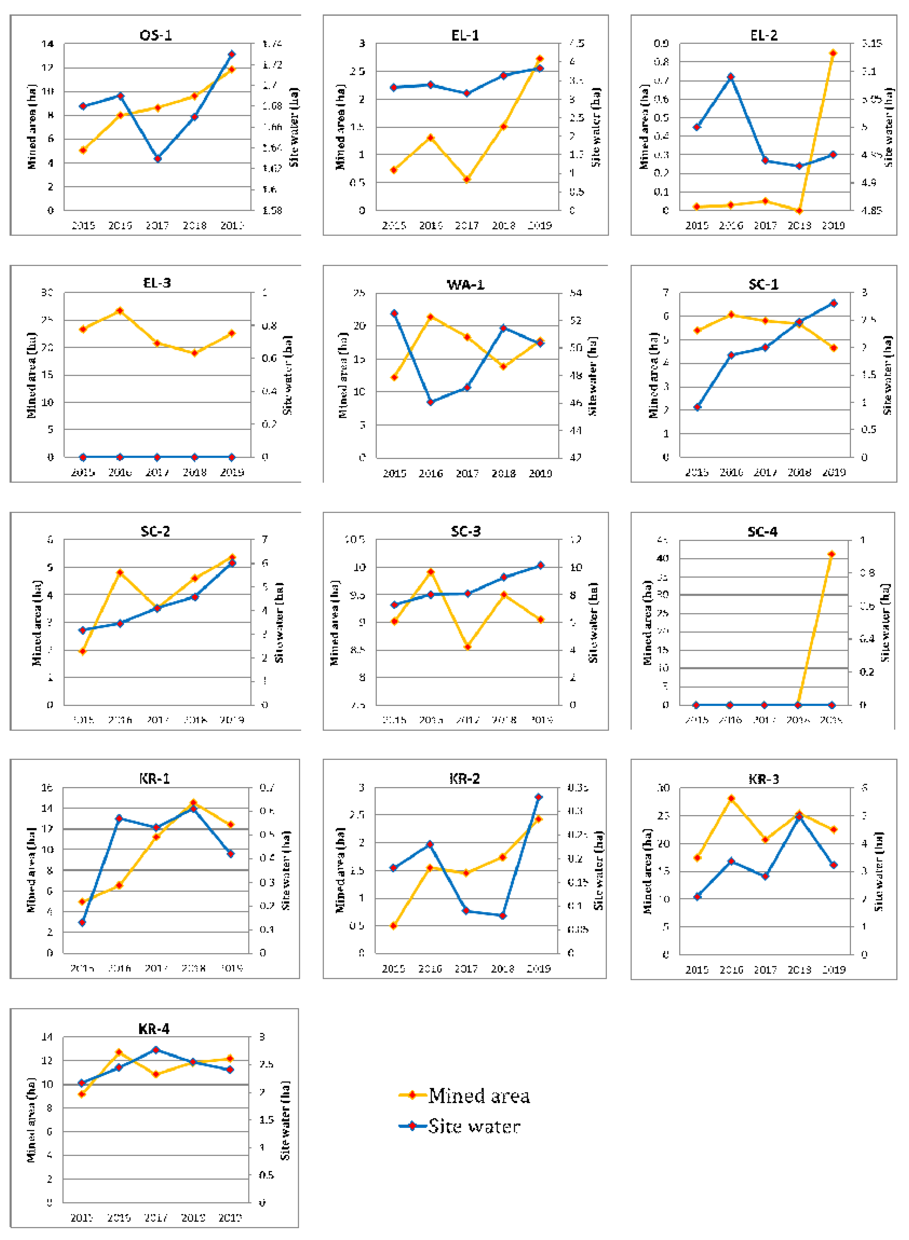
Different trends of changes in both site water and mined areas can be attributed to diverse factors both anthropogenically and naturally. Deductions of factors can be generated by evaluating statistical and visual representations as well as classified images. Mining sites like OS-1 and KR-2 experienced a steady rise in mined areas from 2015 to 2019, which can simply be explained by an increase in mining activities on these sites. New mining sites can also be determined, such as SC-4, which had no evidence of mining until 2019. However, it is paramount to bear in mind that site water should also be non-existence like in SC-4. Unlike SC-4, EL-2 cannot be categorized as a new site due to the presence of site water, which can be explained as having undergone mining activities but colonized by vegetation. The appearance of new mining can be seen in 2019. [43] iterate the fact that previously forested areas after mining are reclaimed into shrublands or grasslands. Mining sites without site water can easily be deduced as well since no evidence of water can be seen in the images for all the years, such as in EL-3 and SC-4. It is important to use both statistical and spatial information for both mined areas and site water to get a clear picture of changes occurring. The change curve for SC-1 (Figure 20) shows a decrease in mined areas when, in fact, images show an increase. The reason for this is the covering of mined areas with site water, which makes the area look smaller. The extent and movement of areas mined can be deduced while areas that have been reclaimed by other land cover can be seen as well.
In effect a deeper look into the analysis is required to fully understand the trends occurring on the surface of the earth. This study fulfills that by providing both statistical and visual representation of the analysis conducted.
Figure 9.
Trends of changes from 2015 to 2019 for the class mined area and site water for all thirteen mining sites.
Figure 9.
Trends of changes from 2015 to 2019 for the class mined area and site water for all thirteen mining sites.
4.3. Importance to Regional Monitoring on Mined Area
The ability to spatially identify and map mineral resources allows for the estimation of resource availability and usage [44]. The initial phase to achieve this using ML is the capbility of satellite data to effectively detect the land cover feature of interest as well as distinguish it from other features. Sentinel’s high spectral capabilities can achieve this in the classification and extraction of mined areas from different land cover features [45]. Additionally, mining areas can be distinguished from vegetative cover, water, bare fields and settlement due to their improved spatial resolution, which allows for a clear distinction between different land cover [46]. NDVI and other spectral indices generated from Sentinel’s multispectral images can be utilized in the establishment of relevant properties affecting mapped sites. [47] compared Landsat and Sentinel in the analysis of surface cover and determined Sentinel provided better results.
Spatial dynamics of areas undergoing mining are subject to rapid changes and hence have been monitored using aerial photography, which is analogous and digitally interpreted [48]. This method is time and cost-intensive and requires a lot of inputs. Application of the SVM classification model to Sentinel, however, offers a time and cost-effective method to spatially analyze mining areas by eliminating transport and input costs. It presents the capability to spatially evaluate a large area, which would require a longer period if conducted manually. Routine observations and data continuity are conducted using Sentinel data for other missions like ASTER, SPOT, and Landsat. Mineral exploration and its trends are analyzed, such as in the study conducted by [49].
The dynamic nature of mining sites due to constant anthropogenic contact requires satellites with faster revisit times like Sentinel [45]. Additionally, classification models based on the SVM algorithm, when applied to Sentinel, are accurate in mapping mined areas [50], thereby providing an effective way to monitor changes continuously. Additionally, mapping of fractures, folds and faults in surface mineralogy can be established and allows for the grouping of minerals into groups. Landscape maps can be generated and provide information on a landscape that otherwise would require on-site analysis.
Application of the SVM model to Sentinel provides information and evaluation into time estimation of the initialization and conclusion of mined activities based on the land cover’s temporal trajectories [51]. Mine reclamation and the periods it began can also be analyzed when mining activities have been concluded. Identifications of changes relating to the impacts of mining about hydrological activities on mining sites through time can be observed. Land cover changes, just like in this study, can be detected based on a time series of sentinel images and can be analyzed based on relevant environmental factors surrounding these land uses.
Evaluation of surface mines can be generated on a bi-weekly, monthly and yearly interval, among others, based on the severity of extraction conducted. Even though Sentinel cannot completely replace field observations, it provides the capability to derive information on past dates, which would not be possible otherwise.
Landscapes which undergo mining activities are pronounced with environmental impacts such as erosion and gullying including those areas in Germany ([52]. Impacts can be mitigated if they can be identified in the first place, and the Sentinel satellite provides such information. Reclamation programs such as the establishment of vegetation on previously mined sites can reduce these impacts. Detection of reclamation and contamination of open mines can be done with Satellite imaging. Impacts on land use with regards to mining activities can be monitored cumulatively due to the multi temporal nature of Sentinel.
Mapping the extent of mining sites as reclaimed mines provide important information in analyzing its ramifications on ecosystem services [43]. The impacts of mining are not always adverse and can be easily mitigated if they can be detected after mining activities have been conducted. Landscape management and planning sustainably can be supported by results derived from change detection methodologies and analysis of land use and land cover behaviour [53].
Trends of land use changes can be predicted based on analysis of previous sentinel data and how land use has changed over time. Ecological restoration, land use planning and management can be effectively handled if the changes to occur over a particular landscape can be predicted. Models such as the Markov Chain is one of the mixed models which can effectively predict the changes to occur in the future [54]. This model possesses the capability of combining long-term predictions and spatial variations to perform land cover simulations, thereby providing the possibility to predict properties of land use [18,35,54]
5. Conclusions
Automated methods of satellite data acquisition, preparation, and processing provide a quick and flexible analysis of the land surfaces and their changes. Geodetic surveys based on sentinel images were executed to understand the dynamics and processes occurring in raw material extraction sites. Spatial information derived was further analyzed quantitatively and qualitatively to establish trends and impacts of these extractions. The initial step of this study was to accurately map areas on the land surface undergoing raw material mining. To achieve this machine learning techniques (RF, SVM, and ANN) were employed, tested, and compared as they have proven to be more efficient than traditional methods in classifying satellite images. Both internal and external validation was conducted to determine the robustness of the above models.
SVM algorithm proved more robust, and with different input factors such as elevation and indices such as the Brightness index, Normalized Differentiation Vegetation Index, and Colourization Index, among others, including band reflectance properties, a model was developed. Application of this method was to different study areas (five areas of interest located widely across Schleswig Flensburg) over five different dates (2015 to 2019). SVM-based classifications were carried out and supplemented with boundary information on parcels of land for mining. The transferability of the model was conclusively proven with the five study areas within the study region. This method, unlike most, utilizes the effectiveness of soil and vegetation indices in distinguishing land cover to improve the accuracy of the model. Results from the model clearly showed accuracies between 90 to 100% for all the images analyzed.
Change detection was performed to further understand the transition of the areas over time and how the landscape has evolved. The extent of areas mined was analyzed to fully understand the trajectory of change or otherwise for these areas. Based on this analysis, it was explicitly proven that the region had experienced an increase in the areas undergoing mining activities over the years. It also showed what magnitude of increase each year had experienced and what had become of abandoned areas. The emergence of new areas mined could also be determined, thereby providing evidence of the starting period of mining, among others
Evidently, after these analyses, it is conclusive that the application of classification algorithms to Sentinel 2 has the capability to provide a wealth of information to assist in the monitoring of raw material extraction. Raw material mining areas can be mapped easily, their spatial extents can be analyzed, their development and trends can be estimated and predicted, and impacts of the extraction activities can be identified with the methods proposed.
Author Contributions
Conceptualization, G.A.; methodology, G.A and K.O.T.; validation, G.A and K.O.T., formal analysis, G.A.; investigation, G.A. and K.O.T. writing—original draft preparation, G.A.; writing—review and editing, K.O.T.; visualization, G.A. All authors have read and agreed to the published version of the manuscript.
Funding
This research received no external funding.
Data Availability Statement
Data used in this study was devirived from Sentinel-2 available at https://dataspace.copernicus.eu/explore-data/data-collections/sentinel-data/sentinel-2.
Acknowledgments
I would like to acknowledge the late Professor Uwe Rammert, whose guidance and inspiration greatly influenced this research.
Conflicts of Interest
The authors declare no conflicts of interest
References
- H. M. Hamada, F. Abed, Z. A. Al-Sadoon, Z. Elnassar, and A. Hassan, “The use of treated desert sand in sustainable concrete: A mechanical and microstructure study,” J. Build. Eng., vol. 79, p. 107843, Nov. 2023. [CrossRef]
- A. J. Sinclair, “Applications of Probability Graphs in Mineral Exploration,” Miner. Explor., 1976.
- J. Blachowski, “Spatial analysis of the mining and transport of rock minerals (aggregates) in the context of regional development,” Environ. Earth Sci., vol. 71, no. 3, pp. 1327–1338, Feb. 2014. [CrossRef]
- A. Torres, J. Brandt, K. Lear, and J. Liu, “A looming tragedy of the sand commons,” Science, vol. 357, no. 6355, pp. 970–971, Sep. 2017. [CrossRef]
- K. Chilamkurthy, A. V. Marckson, S. T. Chopperla, and M. Santhanam, “A statistical overview of sand demand in Asia and Europe.,” 2016.
- J. Lowry, T. Coulthard, M. Saynor, and G. Hancock, “A comparison of landform evolution model predictions with multi-year observations from a rehabilitated landform,” 2020.
- S. K. Karan, S. R. Samadder, and S. K. Maiti, “Assessment of the capability of remote sensing and GIS techniques for monitoring reclamation success in coal mine degraded lands,” J. Environ. Manage., vol. 182, pp. 272–283, Nov. 2016. [CrossRef]
- M. Kampmeier, E. M. Van Der Lee, U. Wichert, and J. Greinert, “Exploration of the munition dumpsite Kolberger Heide in Kiel Bay, Germany: Example for a standardised hydroacoustic and optic monitoring approach,” Cont. Shelf Res., vol. 198, p. 104108, Jul. 2020. [CrossRef]
- W. Leal Filho et al., “Heading towards an unsustainable world: some of the implications of not achieving the SDGs,” Discov. Sustain., vol. 1, no. 1, p. 2, Dec. 2020. [CrossRef]
- G. D. Fachbeitrag Rohstoffsicherung., “Fachbeitrag Rohstoffsicherung,” 2019.
- A. M. Dewan and Y. Yamaguchi, “Using remote sensing and GIS to detect and monitor land use and land cover change in Dhaka Metropolitan of Bangladesh during 1960–2005,” Environ. Monit. Assess., vol. 150, no. 1–4, p. 237, Mar. 2009. [CrossRef]
- A. I. Alastal and A. H. Shaqfa, “GeoAI Technologies and Their Application Areas in Urban Planning and Development: Concepts, Opportunities and Challenges in Smart City (Kuwait, Study Case),” J. Data Anal. Inf. Process., vol. 10, no. 02, pp. 110–126, 2022. [CrossRef]
- B. Huang, B. Zhao, and Y. Song, “Urban land-use mapping using a deep convolutional neural network with high spatial resolution multispectral remote sensing imagery,” Remote Sens. Environ., vol. 214, pp. 73–86, Sep. 2018. [Google Scholar] [CrossRef]
- G. Tasionas et al., “UAV regular mapping focusing on surface mine monitoring,” in Eighth International Conference on Remote Sensing and Geoinformation of the Environment (RSCy2020), K. Themistocleous, S. Michaelides, V. Ambrosia, D. G. Hadjimitsis, and G. Papadavid, Eds., Paphos, Cyprus: SPIE, Aug. 2020, p. 72. [CrossRef]
- P. Tarolli, “High-resolution topography for understanding Earth surface processes: Opportunities and challenges,” Geomorphology, vol. 216, pp. 295–312, Jul. 2014. [CrossRef]
- D. Giordan, Y. S. Hayakawa, F. Nex, and P. Tarolli, “Preface: The use of remotely piloted aircraft systems (RPAS) in monitoring applications and management of natural hazards,” Nat. Hazards Earth Syst. Sci., vol. 18, no. 11, pp. 3085–3087, Nov. 2018. [Google Scholar] [CrossRef]
- A. E. Maxwell, T. A. Warner, M. P. Strager, and M. Pal, “Combining RapidEye Satellite Imagery and Lidar for Mapping of Mining and Mine Reclamation,” Photogramm. Eng. Remote Sens., vol. 80, no. 2, pp. 179–189, Feb. 2014. [CrossRef]
- A. E. Maxwell, T. A. Warner, M. P. Strager, J. F. Conley, and A. L. Sharp, “Assessing machine-learning algorithms and image- and lidar-derived variables for GEOBIA classification of mining and mine reclamation,” Int. J. Remote Sens., vol. 36, no. 4, pp. 954–978, Feb. 2015. [CrossRef]
- H. Schmidt and C. Glaesser, “Multitemporal analysis of satellite data and their use in the monitoring of the environmental impacts of open cast lignite mining areas in Eastern Germany,” Int. J. Remote Sens., vol. 19, no. 12, pp. 2245–2260, Jan. 1998. [CrossRef]
- D. Phiri, M. Simwanda, S. Salekin, V. Nyirenda, Y. Murayama, and M. Ranagalage, “Sentinel-2 Data for Land Cover/Use Mapping: A Review,” Remote Sens., vol. 12, no. 14, p. 2291, Jul. 2020. [Google Scholar] [CrossRef]
- D. C. Duro, S. E. Franklin, and M. G. Dubé, “A comparison of pixel-based and object-based image analysis with selected machine learning algorithms for the classification of agricultural landscapes using SPOT-5 HRG imagery,” Remote Sens. Environ., vol. 118, pp. 259–272, Mar. 2012. [CrossRef]
- L. Qu, Z. Chen, M. Li, J. Zhi, and H. Wang, “Accuracy Improvements to Pixel-Based and Object-Based LULC Classification with Auxiliary Datasets from Google Earth Engine,” Remote Sens., vol. 13, no. 3, p. 453, Jan. 2021. [CrossRef]
- J. Rogan, J. Franklin, and D. A. Roberts, “A comparison of methods for monitoring multitemporal vegetation change using Thematic Mapper imagery,” Remote Sens. Environ., vol. 80, no. 1, pp. 143–156, Apr. 2002. [CrossRef]
- J. F. Mas and J. J. Flores, “The application of artificial neural networks to the analysis of remotely sensed data,” Int. J. Remote Sens., vol. 29, no. 3, pp. 617–663, Feb. 2008. [CrossRef]
- S. M. Yimer, A. Bouanani, N. Kumar, B. Tischbein, and C. Borgemeister, “Comparison of different machine-learning algorithms for land use land cover mapping in a heterogenous landscape over the Eastern Nile river basin, Ethiopia,” Adv. Space Res., vol. 74, no. 5, pp. 2180–2199, Sep. 2024. [CrossRef]
- X. Li, W. Chen, X. Cheng, and L. Wang, “A Comparison of Machine Learning Algorithms for Mapping of Complex Surface-Mined and Agricultural Landscapes Using ZiYuan-3 Stereo Satellite Imagery,” Remote Sens., vol. 8, no. 6, p. 514, Jun. 2016. [CrossRef]
- K. Gee, “Offshore wind power development as affected by seascape values on the German North Sea coast,” Land Use Policy, vol. 27, no. 2, pp. 185–194, Apr. 2010. [CrossRef]
- Q. Wang, W. Shi, Z. Li, and P. M. Atkinson, “Fusion of Sentinel-2 images,” Remote Sens. Environ., vol. 187, pp. 241–252, Dec. 2016. [CrossRef]
- O. Hagolle, M. Huc, D. Villa Pascual, and G. Dedieu, “A Multi-Temporal and Multi-Spectral Method to Estimate Aerosol Optical Thickness over Land, for the Atmospheric Correction of FormoSat-2, LandSat, VENμS and Sentinel-2 Images,” Remote Sens., vol. 7, no. 3, pp. 2668–2691, Mar. 2015. [Google Scholar] [CrossRef]
- R. Khatami, G. Mountrakis, and S. V. Stehman, “A meta-analysis of remote sensing research on supervised pixel-based land-cover image classification processes: General guidelines for practitioners and future research,” Remote Sens. Environ., vol. 177, pp. 89–100. May; 2016. [CrossRef]
- M.-R. Rujoiu-Mare, B. Olariu, B.-A. Mihai, C. Nistor, and I. Săvulescu, “Land cover classification in Romanian Carpathians and Subcarpathians using multi-date Sentinel-2 remote sensing imagery,” Eur. J. Remote Sens., vol. 50, no. 1, pp. 496–508, Jan. 2017. [CrossRef]
- T. Blaschke et al., “Geographic Object-Based Image Analysis – Towards a new paradigm,” ISPRS J. Photogramm. Remote Sens., vol. 87, pp. 180–191, Jan. 2014. [CrossRef]
- X. Li and Y. Tang, “Two-dimensional nearest neighbor classification for agricultural remote sensing,” Neurocomputing, vol. 142, pp. 182–189, Oct. 2014. [CrossRef]
- G. M. Foody and A. Mathur, “A relative evaluation of multiclass image classification by support vector machines,” IEEE Trans. Geosci. Remote Sens., vol. 42, no. 6, pp. 1335–1343, Jun. 2004. [CrossRef]
- M. J. Cracknell and A. M. Reading, “Geological mapping using remote sensing data: A comparison of five machine learning algorithms, their response to variations in the spatial distribution of training data and the use of explicit spatial information,” Comput. Geosci., vol. 63, pp. 22–33, Feb. 2014. [CrossRef]
- C. Huang, L. S. Davis, and J. R. G. Townshend, “An assessment of support vector machines for land cover classification,” Int. J. Remote Sens., vol. 23, no. 4, pp. 725–749, Jan. 2002. [Google Scholar] [CrossRef]
- R. S. De Fries, M. Hansen, J. R. G. Townshend, and R. Sohlberg, “Global land cover classifications at 8 km spatial resolution: The use of training data derived from Landsat imagery in decision tree classifiers,” Int. J. Remote Sens., vol. 19, no. 16, pp. 3141–3168, Jan. 1998. [CrossRef]
- C. Gómez, J. C. White, and M. A. Wulder, “Optical remotely sensed time series data for land cover classification: A review,” ISPRS J. Photogramm. Remote Sens., vol. 116, pp. 55–72, Jun. 2016. [Google Scholar] [CrossRef]
- C. Folke, L. Pritchard, Jr., F. Berkes, J. Colding, and U. Svedin, “The Problem of Fit between Ecosystems and Institutions: Ten Years Later,” Ecol. Soc., vol. 12, no. 1, p. art30, 2007. [CrossRef]
- J. F. Knight, B. P. Tolcser, J. M. Corcoran, and L. P. Rampi, “The Effects of Data Selection and Thematic Detail on the Accuracy of High Spatial Resolution Wetland Classifications,” Photogramm. Eng., 2013.
- J. Corcoran, J. Knight, K. Pelletier, L. Rampi, and Y. Wang, “The Effects of Point or Polygon Based Training Data on RandomForest Classification Accuracy of Wetlands,” Remote Sens., vol. 7, no. 4, pp. 4002–4025, Apr. 2015. [CrossRef]
- P. A. Townsend, D. P. Helmers, C. C. Kingdon, B. E. McNeil, K. M. De Beurs, and K. N. Eshleman, “Changes in the extent of surface mining and reclamation in the Central Appalachians detected using a 1976–2006 Landsat time series,” Remote Sens. Environ., vol. 113, no. 1, pp. 62–72, Jan. 2009. [CrossRef]
- J. A. Simmons et al., “FOREST TO RECLAIMED MINE LAND USE CHANGE LEADS TO ALTERED ECOSYSTEM STRUCTURE AND FUNCTION,” Ecol. Appl., vol. 18, no. 1, pp. 104–118, Jan. 2008. [CrossRef]
- H. M. Rajesh, “Application of remote sensing and GIS in mineral resource mapping ɻ An overview,” 2004.
- M. Drusch et al., “Sentinel-2: ESA’s Optical High-Resolution Mission for GMES Operational Services,” Remote Sens. Environ., vol. 120, pp. 25–36, May 2012. [CrossRef]
- A. Whyte, K. P. Ferentinos, and G. P. Petropoulos, “A new synergistic approach for monitoring wetlands using Sentinels -1 and 2 data with object-based machine learning algorithms,” Environ. Model. Softw., vol. 104, pp. 40–54, Jun. 2018. [CrossRef]
- L. Korhonen, Hadi, P. Packalen, and M. Rautiainen, “Comparison of Sentinel-2 and Landsat 8 in the estimation of boreal forest canopy cover and leaf area index,” Remote Sens. Environ., vol. 195, pp. 259–274, Jun. 2017. [CrossRef]
- S. R. Schneider, D. F. McGINNIS, and G. Stephens, “Monitoring Africa’s Lake Chad basin with LANDSAT and NOAA satellite data,” Int. J. Remote Sens., vol. 6, no. 1, pp. 59–73, Jan. 1985. [CrossRef]
- F. F. Sabins, “Remote sensing for mineral exploration,” 1999.
- N.-T. Son, C.-F. Chen, C.-R. Chen, and V.-Q. Minh, “Assessment of Sentinel-1A data for rice crop classification using random forests and support vector machines,” Geocarto Int., pp. 1–15, Feb. 2017. [CrossRef]
- A. E. Maxwell and T. A. Warner, “Differentiating mine-reclaimed grasslands from spectrally similar land cover using terrain variables and object-based machine learning classification,” Int. J. Remote Sens., vol. 36, no. 17, pp. 4384–4410, Sep. 2015. [CrossRef]
- E. Hildmann and M. Wonsche, “Lignite mining and its after-effects on the Central German landscape”.
- A. M. Dewan and Y. Yamaguchi, “Using remote sensing and GIS to detect and monitor land use and land cover change in Dhaka Metropolitan of Bangladesh during 1960–2005,” Environ. Monit. Assess., vol. 150, no. 1–4, p. 237, Mar. 2009. [CrossRef]
- S. W. Myint and L. Wang, “Multicriteria decision approach for land use land cover change using Markov chain analysis and a cellular automata approach,” Can. J. Remote Sens., vol. 32, no. 6, pp. 390–404, Dec. 2006. [CrossRef]
Figure 1.
Geographic and spatial location of the study areas.
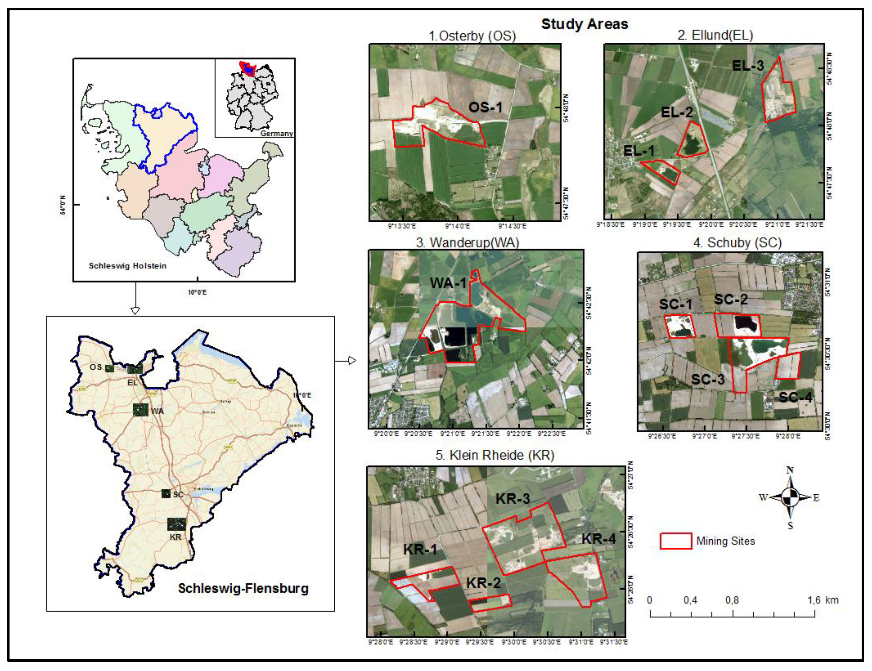
Figure 2.
The overall workflow of methodologies used to build a model, map and analyze mining sites.
Figure 2.
The overall workflow of methodologies used to build a model, map and analyze mining sites.
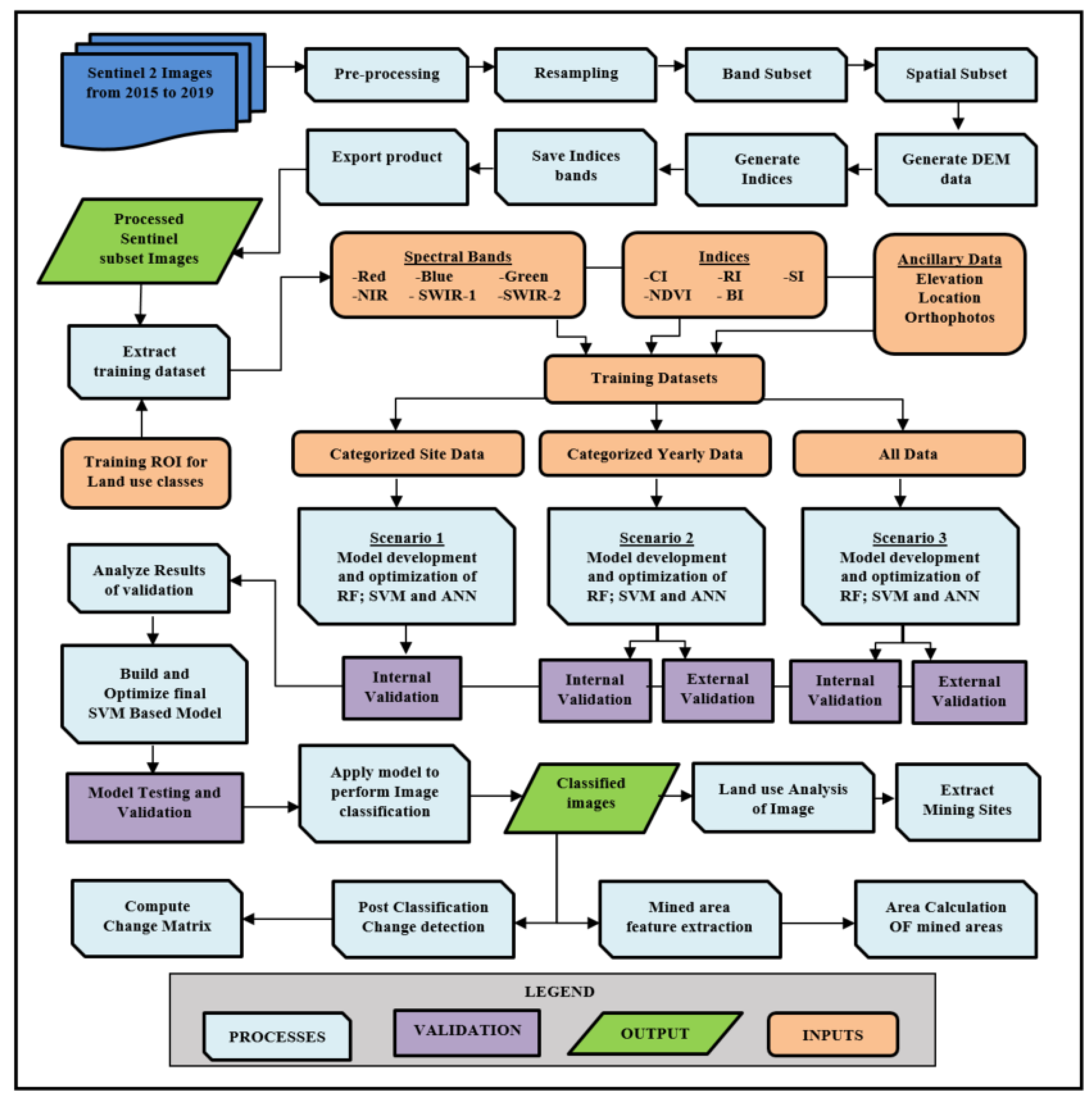
Figure 3.
Classification results derived from the RF, SVM and ANN model based on 2015 training data for classifying study area from 2015 images.
Figure 3.
Classification results derived from the RF, SVM and ANN model based on 2015 training data for classifying study area from 2015 images.
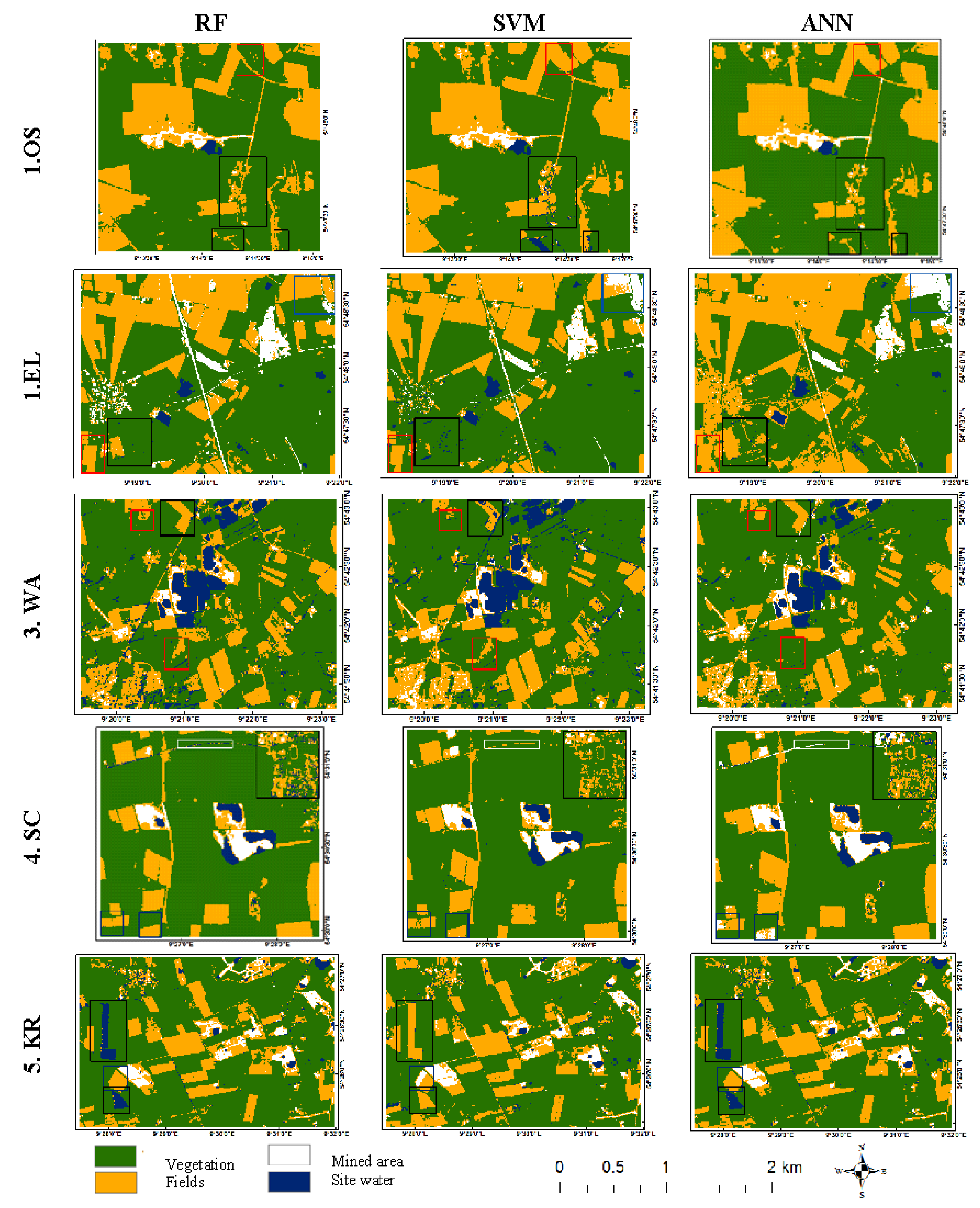
Figure 4.
Graphs showing the comparison between model accuracies of the RF, SVM and ANN model in percentages for the five study areas.
Figure 4.
Graphs showing the comparison between model accuracies of the RF, SVM and ANN model in percentages for the five study areas.
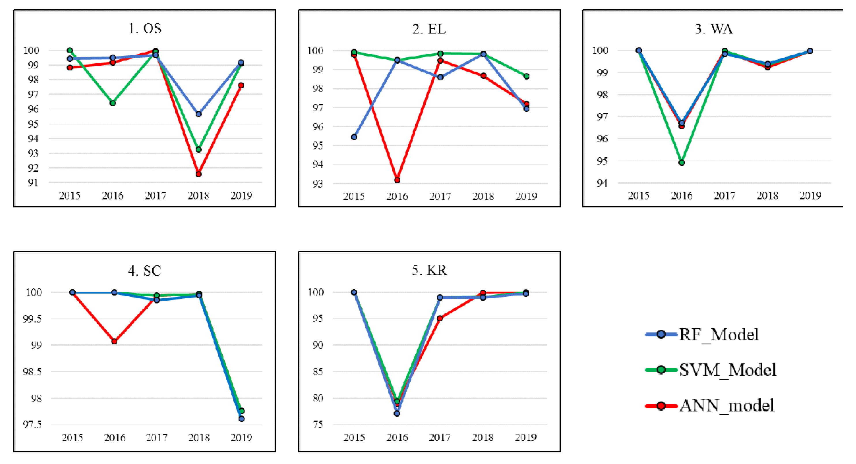
Figure 5.
The confusion Matrix image in pixels for the three models (RF, SVM, ANN) for classification of the 2019 images for all the study areas.
Figure 5.
The confusion Matrix image in pixels for the three models (RF, SVM, ANN) for classification of the 2019 images for all the study areas.
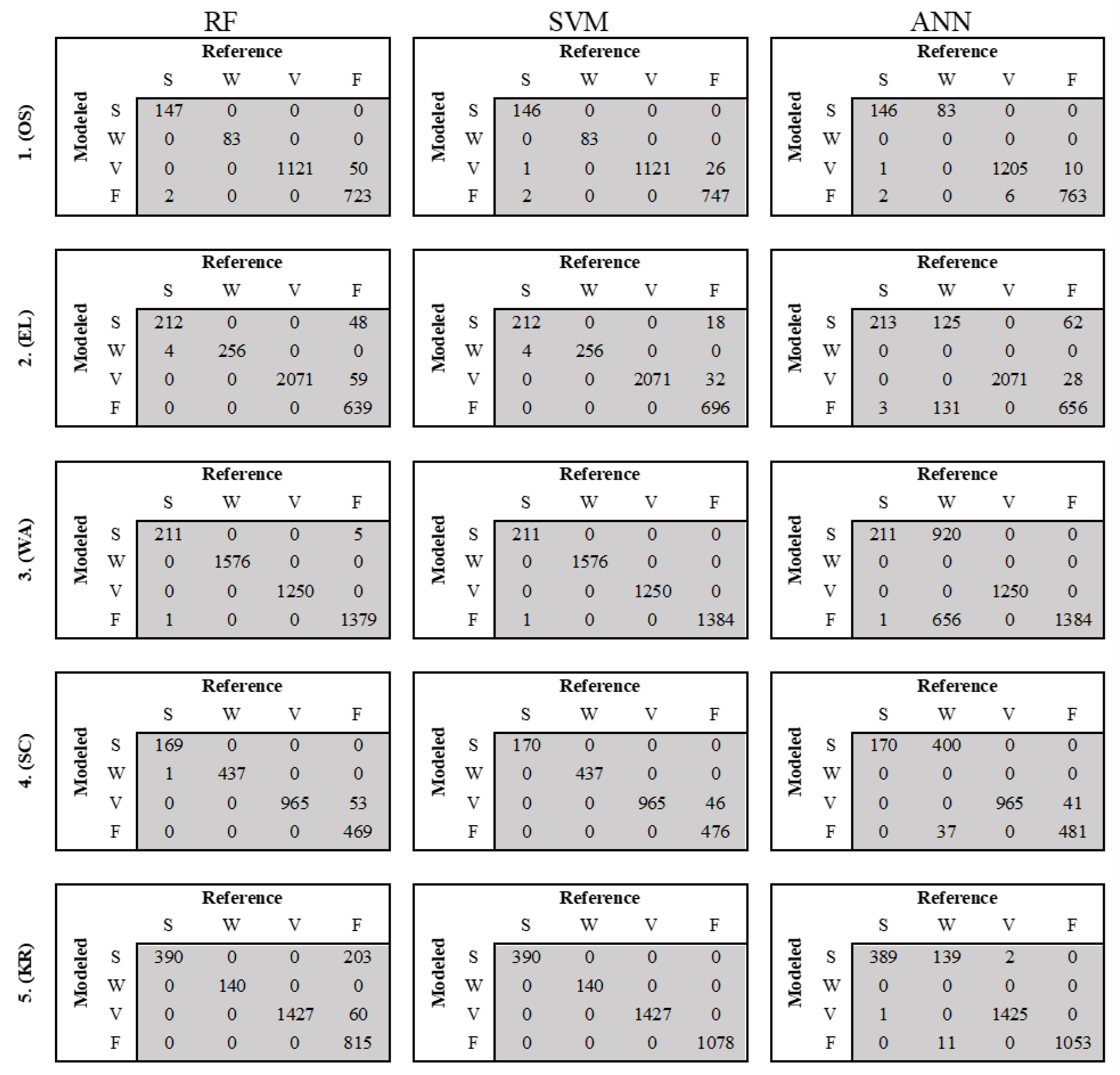
Figure 8.
Land cover maps for study area Schuby for 2015-2019.
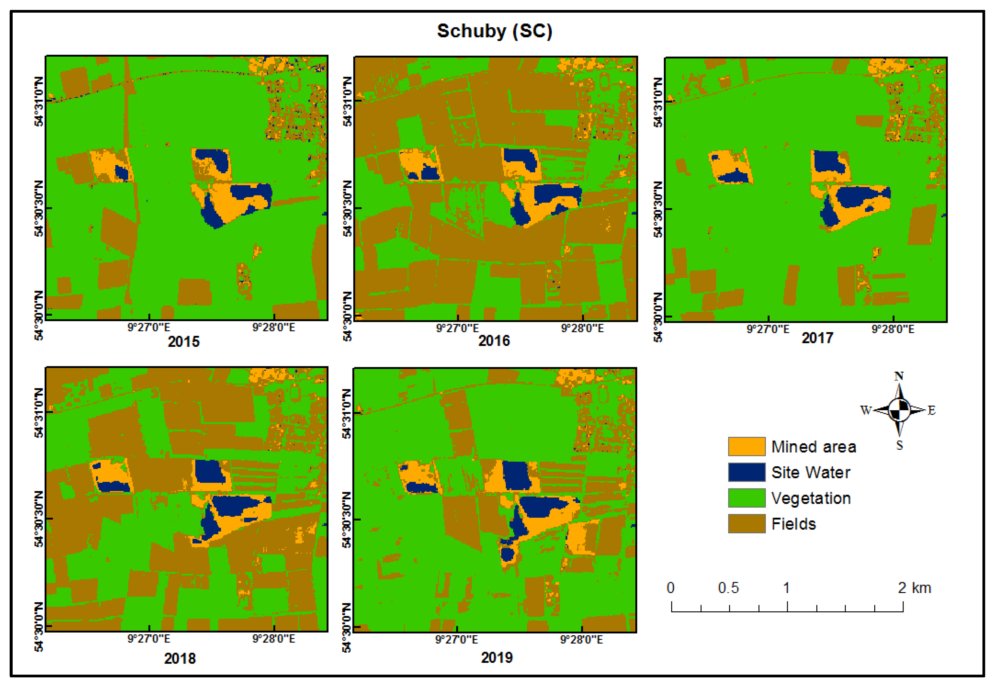
Figure 9.
Reflectance and index values of the different bands and indices for the different land cover classes.
Figure 9.
Reflectance and index values of the different bands and indices for the different land cover classes.
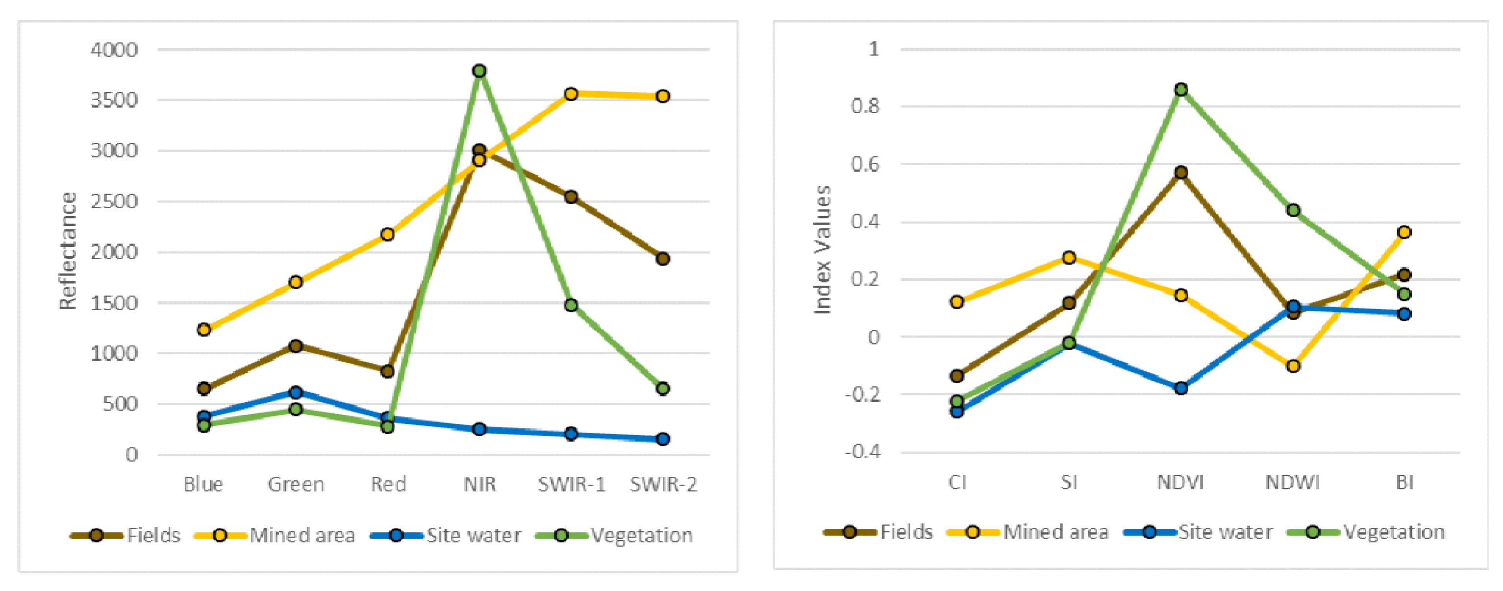

Table 1.
Study areas including their attributes such as name, area, pixels, number of mines, and presence of water.
Table 1.
Study areas including their attributes such as name, area, pixels, number of mines, and presence of water.
| Study Area | 1(OS) | 2(EL) | 3(WA) | 4(SC) | 5(KR) |
|---|---|---|---|---|---|
| Name | Osterby | Ellund | Wanderup | Schuby | Klein Rheide |
| Area (sq. km) | 4322.8 | 12870.2 | 13258.7 | 5684 | 15600.9 |
| Pixels (10*10) | 214*202 | 406*317 | 403*329 | 245*232 | 483*323 |
| No. of mines | 1 | 3 | 1 | 4 | 4 |
| Water | Yes | No | Yes | Yes | Yes |
Table 2.
Attributes of Sentinel tiles downloaded with their dates and respective tile names.
| Year | Date Sensed | Tile Name |
|---|---|---|
| 2015 | 22.08.2015 | S2A_MSIL1C_20150822T104036_N0204_R008_T32UNF_20150822T104035 |
| 2016 | 04.06.2016 | S2A_MSIL1C_20160604T103032_N0202_R108_T32UNF_20160604T103026 |
| 2017 | 19.07.2017 | S2A_MSIL1C_20170719T103021_N0205_R108_T32UNF_20170719T103023 |
| 2018 | 25.05.2018 | S2A_MSIL1C_20180525T103021_N0206_R108_T32UNF_20180525T124252 |
| 2019 | 29.06.2019 | S2A_MSIL1C_20180525T103021_N0206_R108_T32UNF_20180525T124252 |
Table 3.
Attributes of Indices used as variable inputs to train the three classifiers, including their property and formula.
Table 3.
Attributes of Indices used as variable inputs to train the three classifiers, including their property and formula.
| Indices | Property | Formula |
|---|---|---|
| Normalized Difference Vegetation Index (NDVI) | Health and amount of Vegetation | (NIR-R) / (NIR + R) |
| Brightness Index (BI) | Average reflectance magnitude | ((R2 + G2 + B2) / 3)0.5 |
| Coloration Index (CI) | Soil colour | (R-G) / (R + G) |
| Saturation Index (SI) | Spectral slope | (R-B) / (R + B) |
| Redness Index (RI) | Hematite content | R2 / (B * G3) |
Table 4.
Accuracy and Kappa results for the three classifiers (RF, SVM, ANN) based on individually trained Models.
Table 4.
Accuracy and Kappa results for the three classifiers (RF, SVM, ANN) based on individually trained Models.
| Data | Random Forest | Support Vector Machine | Neural Network | |||
|---|---|---|---|---|---|---|
| Accuracy | Kappa | Accuracy | Kappa | Accuracy | Kappa | |
| 2015 | ||||||
| OS | 0.9991 | 0.9986 | 0.9994 | 0.9991 | 0.9994 | 0.9991 |
| EL | 0.9958 | 0.9932 | 0.9939 | 0.9900 | 0.9912 | 0.9858 |
| WA | 0.9988 | 0.9982 | 0.9901 | 0.9852 | 0.9980 | 0.9971 |
| SC | 0.9978 | 0.9970 | 0.9985 | 0.9978 | 0.9977 | 0.9967 |
| KR | 0.9993 | 0.9989 | 0.9973 | 0.9959 | 0.9986 | 0.9980 |
| 2016 | ||||||
| OS | 0.9984 | 0.9973 | 0.9971 | 0.9949 | 0.9949 | 0.9911 |
| EL | 0.9963 | 0.9934 | 0.9946 | 0.9904 | 0.9954 | 0.9918 |
| WA | 0.9967 | 0.9954 | 0.9956 | 0.9938 | 0.9957 | 0.9939 |
| SC | 0.9952 | 0.9927 | 0.9932 | 0.9897 | 0.9940 | 0.9910 |
| KR | 0.9847 | 0.9757 | 0.9781 | 0.9652 | 0.9781 | 0.9653 |
| 2017 | ||||||
| OS | 0.9910 | 0.9844 | 0.9828 | 0.9702 | 0.9853 | 0.9745 |
| EL | 0.9985 | 0.9974 | 0.9979 | 0.9964 | 0.9984 | 0.9973 |
| WA | 0.9951 | 0.9930 | 0.9919 | 0.9884 | 0.9930 | 0.9900 |
| SC | 0.9997 | 0.9994 | 0.9997 | 0.9994 | 0.9994 | 0.9990 |
| KR | 0.9981 | 0.9968 | 0.9967 | 0.9944 | 0.9967 | 0.9944 |
| 2018 | ||||||
| OS | 0.8465 | 0.7303 | 0.8477 | 0.7313 | 0.8597 | 0.7524 |
| EL | 0.9980 | 0.9966 | 0.9958 | 0.9929 | 0.9959 | 0.9930 |
| WA | 0.9963 | 0.9942 | 0.9756 | 0.9641 | 0.9843 | 0.9768 |
| SC | 0.9968 | 0.9949 | 0.9966 | 0.9946 | 0.9954 | 0.9927 |
| KR | 0.9997 | 0.9995 | 0.9993 | 0.9989 | 0.9995 | 0.9993 |
| 2019 | ||||||
| OS | 0.9577 | 0.9252 | 0.9087 | 0.8384 | 0.9205 | 0.8593 |
| EL | 0.9970 | 0.9915 | 0.9887 | 0.9675 | 0.9956 | 0.9874 |
| WA | 0.9973 | 0.9960 | 0.9938 | 0.9911 | 0.9931 | 0.9900 |
| SC | 0.9779 | 0.9624 | 0.9666 | 0.9436 | 0.9747 | 0.9569 |
| KR | 0.9889 | 0.9809 | 0.9858 | 0.9756 | 0.9856 | 0.9753 |
Table 5.
Accuracy and Kappa results of the RF, SVM and ANN model trained with yearly data based on internal accuracy statistics.
Table 5.
Accuracy and Kappa results of the RF, SVM and ANN model trained with yearly data based on internal accuracy statistics.
| Year | Random Forest | Support Vector Machine | Neural Network | |||
|---|---|---|---|---|---|---|
| Accuracy | Kappa | Accuracy | Kappa | Accuracy | Kappa | |
| 2015 | 0.9984 | 0.9978 | 0.9980 | 0.9971 | 0.9966 | 0.9951 |
| 2016 | 0.9989 | 0.9983 | 0.9900 | 0.9835 | 0.9924 | 0.9883 |
| 2017 | 0.9990 | 0.9982 | 0.9966 | 0.9948 | 0.9945 | 0.9914 |
| 2018 | 0.9871 | 0.9802 | 0.9754 | 0.9620 | 0.9762 | 0.9632 |
| 2019 | 0.9951 | 0.9919 | 0.9715 | 0.9526 | 0.9632 | 0.9386 |
Table 6.
Kappa Index and Overall accuracy for the RF, SVM and ANN model based on the combination of all training data.
Table 6.
Kappa Index and Overall accuracy for the RF, SVM and ANN model based on the combination of all training data.
| Model | Accuracy | Kappa |
|---|---|---|
| RF | 0.9945 | 0.9916 |
| SVM | 0.9781 | 0.9663 |
| ANN | 0.9639 | 0.9399 |
Table 7.
Accuracy; Kappa and Specificity results based on external validation of the RF, SVM and ANN model for the five study area from 2015 -2019.
Table 7.
Accuracy; Kappa and Specificity results based on external validation of the RF, SVM and ANN model for the five study area from 2015 -2019.
| Data | Random Forest | Support Vector Machine | Neural Network | ||||||
|---|---|---|---|---|---|---|---|---|---|
| Accuracy | Kappa | Specificity | Accuracy | Kappa | Specificity | Accuracy | Kappa | Specificity | |
| 2015 | |||||||||
| 1. OS | 0.987 | 0.975 | 1 | 0.929 | 0.853 | 1 | 0.843 | 0.689 | 0.974 |
| 2. EL | 0.999 | 0.999 | 1 | 1 | 1 | 1 | 0.977 | 0.958 | 0.958 |
| 3. WA | 1 | 1 | 1 | 1 | 1 | 1 | 0.629 | 0.533 | 0.661 |
| 4. SC | 0.995 | 0.994 | 1 | 1 | 1 | 1 | 0.868 | 0.799 | 0.896 |
| 5. KR | 0.811 | 0.720 | 0.720 | 1 | 1 | 1 | 0.972 | 0.953 | 0.974 |
| 2016 | |||||||||
| 1. OS | 0.999 | 0.998 | 0.999 | 0.999 | 0.999 | 1 | 0.936 | 0.886 | 0.972 |
| 2. EL | 0.998 | 0.996 | 0.998 | 0.999 | 0.998 | 0.999 | 0.955 | 0.923 | 0.959 |
| 3. WA | 0.967 | 0.952 | 0.999 | 0.967 | 0.952 | 0.999 | 0.682 | 0.573 | 0.731 |
| 4. SC | 1 | 1 | 1 | 0.999 | 0.998 | 0.998 | 0.903 | 0.826 | 0.908 |
| 5. KR | 0.627 | 0.350 | 0.829 | 0.777 | 0.542 | 0.989 | 0.757 | 0.492 | 0.975 |
| 2017 | |||||||||
| 1. OS | 0.996 | 0.992 | 1 | 0.995 | 0.990 | 1 | 0.976 | 0.955 | 0.978 |
| 2. EL | 0.946 | 0.904 | 0.972 | 0.954 | 0.917 | 1 | 0.936 | 0.885 | 0.964 |
| 3. WA | 0.988 | 0.982 | 1 | 0.981 | 0.971 | 1 | 0.653 | 0.520 | 0.932 |
| 4. SC | 0.999 | 0.999 | 1 | 1 | 1 | 1 | 0.843 | 0.764 | 0.838 |
| 5. KR | 0.881 | 0.812 | 0.896 | 0.99 | 0.983 | 1 | 0.957 | 0.925 | 0.986 |
| 2018 | |||||||||
| 1. OS | 0.918 | 0.845 | 1 | 0.980 | 0.963 | 1 | 0.943 | 0.893 | 0.971 |
| 2. EL | 0.998 | 0.997 | 0.999 | 0.998 | 0.997 | 1 | 0.938 | 0.897 | 0.960 |
| 3. WA | 0.994 | 0.991 | 1 | 0.994 | 0.990 | 0.999 | 0.684 | 0.540 | 0.743 |
| 4. SC | 0.999 | 0.998 | 0.998 | 0.993 | 0.989 | 0.993 | 0.866 | 0.733 | 0.805 |
| 5. KR | 0.858 | 0.769 | 0.850 | 1 | 1 | 1 | 0.968 | 0.939 | 0.991 |
| 2019 | |||||||||
| 1. OS | 0.977 | 0.959 | 1 | 0.987 | 0.977 | 1 | 0.954 | 0.920 | 0.960 |
| 2. EL | 0.966 | 0.937 | 0.984 | 0.987 | 0.970 | 0.994 | 0.894 | 0.802 | 0.782 |
| 3. WA | 0.999 | 0.998 | 0.999 | 0.999 | 0.999 | 1 | 0.643 | 0.533 | 0.782 |
| 4. SC | 0.974 | 0.962 | 1 | 0.978 | 0.967 | 1 | 0.772 | 0.672 | 0.792 |
| 5. KR | 0.913 | 0.866 | 0.866 | 1 | 1 | 1 | 0.945 | 0.912 | 0.951 |
Table 8.
Accuracy and F1-score results based on external validation of the SVM model from 2015 -2019.
Table 8.
Accuracy and F1-score results based on external validation of the SVM model from 2015 -2019.
| Year | Osterby (OS) | Ellund (EL) | Wanderup (WA) | Schuby (SC) | Klein Rheide (KR) | ||||||
|---|---|---|---|---|---|---|---|---|---|---|---|
| Accuracy | F1 score | Accuracy | F1 score | Accuracy | F1 score | Accuracy | F1 score | Accuracy | F1 score | ||
| 2015 | 0.92 | 0.98 | 1 | 1 | 1 | 1 | 1 | 1 | 1 | 1 | |
| 2016 | 0.99 | 0.98 | 0.99 | 0.98 | 0.97 | 0.97 | 0.99 | 0.98 | 0.78 | 0.77 | |
| 2017 | 0.99 | 0.99 | 0.95 | 0.99 | 0.98 | 0.98 | 1 | 1 | 0.99 | 0.99 | |
| 2018 | 0.98 | 0.99 | 0.99 | 0.97 | 0.99 | 0.96 | 0.99 | 0.94 | 0.99 | 0.99 | |
| 2019 | 0.99 | 0.98 | 0.98 | 0.91 | 0.99 | 0.99 | 0.98 | 1 | 1 | 1 | |
Table 9.
Summary of variable combinations used to build the SVM model, and their accuracies and kappa.
Table 9.
Summary of variable combinations used to build the SVM model, and their accuracies and kappa.
| Variable Combinations | Accuracy | Kappa |
|---|---|---|
| Red, Green, Blue, NIR | 0.968 | 0.940 |
| Red, Green, Blue, NIR, SWIR-1 | 0.970 | 0.944 |
| Red, Green, Blue, NIR, SWIR-1, SWIR-2 | 0.981 | 0.964 |
| Red, Green, Blue, NIR, SWIR-1, SWIR-2, CI | 0.980 | 0.963 |
| Red, Green, Blue, NIR, SWIR-1, SWIR-2, CI, RI | 0.980 | 0.963 |
| Red, Green, Blue, NIR, SWIR-1, SWIR-2, CI, RI, SI | 0.977 | 0.957 |
| Red, Green, Blue, NIR, SWIR-1, SWIR-2, CI, RI, SI, NDVI | 0.982 | 0.967 |
| Red, Green, Blue, NIR, SWIR-1, SWIR-2, CI, RI, SI, NDVI, BI | 0.983 | 0.968 |
| Red, Green, Blue, NIR, SWIR-1, SWIR-2, CI, RI, SI, NDVI, BI, Elevation | 0.984 | 0.970 |
Table 10.
Accuracy and Kappa results of the RF, SVM and ANN model trained with yearly data based on internal accuracy statistics.
Table 10.
Accuracy and Kappa results of the RF, SVM and ANN model trained with yearly data based on internal accuracy statistics.
| 2015 | 2016 | 2017 | 2018 | 2019 | |||||||
|---|---|---|---|---|---|---|---|---|---|---|---|
| Land cover | Area (km2) |
% of Area |
Area (km2) |
% of Area |
Area (km2) |
% of Area |
Area (km2) |
% of Area |
Area (km2) |
% of Area |
|
| Osterby (OS) | |||||||||||
| Mined area | 0.06 | 1.39 | 0.09 | 2.08 | 0.09 | 2.08 | 0.1 | 2.31 | 0.1 | 2.31 | |
| Water | 0.03 | 0.69 | 0.02 | 0.46 | 0.02 | 0.46 | 0.02 | 0.46 | 0.02 | 0.46 | |
| Vegetation | 3.58 | 82.87 | 2.41 | 55.79 | 3.22 | 74.36 | 2.15 | 49.77 | 3.04 | 70.37 | |
| Fields | 0.65 | 15.05 | 1.8 | 41.67 | 1 | 23.09 | 2.05 | 47.45 | 1.16 | 26.85 | |
| Ellund (EL) | |||||||||||
| Mined area | 0.36 | 2.8 | 0.33 | 2.56 | 0.27 | 2.1 | 0.34 | 2.64 | 0.38 | 2.95 | |
| Water | 0.17 | 1.32 | 0.15 | 1.17 | 0.13 | 1.01 | 0.16 | 1.24 | 0.13 | 1.01 | |
| Vegetation | 8.08 | 62.83 | 9.11 | 70.78 | 8.97 | 69.7 | 9.66 | 75.06 | 9.96 | 77.39 | |
| Fields | 4.25 | 33.05 | 3.28 | 25.49 | 3.5 | 27.2 | 2.71 | 21.06 | 2.4 | 18.65 | |
| Wanderup (WA) | |||||||||||
| Mined area | 0.29 | 2.19 | 0.31 | 2.34 | 0.3 | 2.26 | 0.29 | 2.19 | 0.34 | 2.44 | |
| Water | 0.66 | 4.98 | 0.63 | 4.75 | 0.61 | 4.6 | 0.65 | 4.9 | 0.62 | 4.44 | |
| Vegetation | 10.47 | 78.96 | 5.96 | 44.95 | 10.54 | 79.49 | 6.35 | 47.85 | 9.77 | 69.99 | |
| Fields | 1.84 | 13.88 | 6.36 | 47.96 | 1.81 | 13.65 | 5.98 | 45.06 | 3.23 | 23.14 | |
| Schuby (SC) | |||||||||||
| Mined area | 0.24 | 4.23 | 0.25 | 4.4 | 0.26 | 4.57 | 0.26 | 4.57 | 0.31 | 5.46 | |
| Water | 0.15 | 2.64 | 0.14 | 2.46 | 0.15 | 2.64 | 0.16 | 2.82 | 0.17 | 2.99 | |
| Vegetation | 4.21 | 74.12 | 1.69 | 29.75 | 4.51 | 79.26 | 2.27 | 39.96 | 3.83 | 67.43 | |
| Fields | 1.08 | 19.01 | 3.6 | 63.38 | 0.77 | 13.53 | 2.99 | 52.64 | 1.37 | 24.12 | |
| Klein Rheide (KR) | |||||||||||
| Mined area | 0.7 | 4.49 | 0.81 | 5.19 | 0.82 | 5.26 | 0.87 | 5.57 | 0.9 | 5.77 | |
| Water | 0.23 | 1.47 | 0.18 | 1.15 | 0.18 | 1.15 | 0.22 | 1.41 | 0.18 | 1.15 | |
| Vegetation | 11.38 | 72.95 | 7.08 | 45.38 | 11.47 | 73.53 | 7.17 | 45.93 | 10.48 | 67.18 | |
| Fields | 3.29 | 21.09 | 7.53 | 48.27 | 3.13 | 20.06 | 7.35 | 47.09 | 4.04 | 25.9 | |
Disclaimer/Publisher’s Note: The statements, opinions and data contained in all publications are solely those of the individual author(s) and contributor(s) and not of MDPI and/or the editor(s). MDPI and/or the editor(s) disclaim responsibility for any injury to people or property resulting from any ideas, methods, instructions or products referred to in the content. |
© 2025 by the authors. Licensee MDPI, Basel, Switzerland. This article is an open access article distributed under the terms and conditions of the Creative Commons Attribution (CC BY) license (http://creativecommons.org/licenses/by/4.0/).
Copyright: This open access article is published under a Creative Commons CC BY 4.0 license, which permit the free download, distribution, and reuse, provided that the author and preprint are cited in any reuse.


