
Submitted:
06 July 2025
Posted:
07 July 2025
You are already at the latest version
Abstract
Forecasts often fail not because they are wrong, but because the people who need them cannot retrieve the signal in time. \textit{Retrieval collapse}, the breakdown between forecast availability and observer recognition, creates these failures. We present Observer-Dependent Entropy Retrieval (ODER), a Markovian and entropy-based framework that models information uptake as observer-specific convergence shaped by institutional latency, update cadence, and hierarchical complexity. A proper-time indexed retrieval law with a hyperbolic-tangent profile tracks when each observer crosses the recognition threshold. Hindcast analyses of the 2023 Antarctic sea-ice collapse, Hurricane Ida in 2021, and the 2020 Siberian heatwave show that observers with identical forecasts can differ by 4.3 to 15 days in recognizing the same tipping point. ODER prevents retrieval collapse in the slowest institutional classes, restoring timely awareness. Compared to traditional pipelines such as EnKF and 4D-Var, the framework explains an additional 33 to 70 percent of retrieval variance when evaluated with Brier scores, root-mean-square error, and observability thresholds. A five-phase validation roadmap couples retrospective overlays with synthetic tipping scenarios and institutional calibration, providing a reproducible path to operational deployment. All benchmark results and simulations are reproduced in an open-source notebook. ODER does not replace physical models; it restores retrieval fidelity as a missing dimension, enabling equitable and timely action under cascading climate risk.
Keywords:
observer-dependent entropy
; climate forecasting
; tipping points
; data latency
; Bayesian inference
; Markov processes
; science-policy interface
; decision latency
; collective intelligence
; information asymmetry
Plain Language Summary
Climate forecasts sometimes fail to protect people, not because the science is wrong, but because the warning never reaches the right person in time. Different institutions, such as weather centers, emergency managers, and policymakers, process information at different speeds. Some receive updates in real time, while others may wait days for internal reviews and approval chains. These delays allow one group to act early, while another misses the signal entirely.
We introduce a framework called Observer-Dependent Entropy Retrieval (ODER) to track how fast different observers recognize the same climate event. Using three real cases, a deadly hurricane, a historic heatwave, and an Antarctic sea ice collapse, we show that observers can diverge by several days even when they share identical forecast data. ODER reveals these retrieval gaps by modeling how information moves, or stalls, across institutions. It does not replace forecast models; instead, it shows who retrieves their warnings and when.
By making retrieval gaps visible, ODER guides the design of alert systems that help everyone act before it is too late.
1. Introduction
Forecasts often fail not because they are wrong, but because the people who need them never see the warning in time. Retrieval collapse, the breakdown between forecast availability and observer recognition, lies at the heart of this problem. Forecasts are interpreted, acted upon, or ignored through heterogeneous institutional pathways, with update frequencies, data lags, and decision-making windows varying across observer classes. Most operational forecasting systems, however, implicitly assume homogeneous information processing across scientists, policymakers, and the public. This assumption creates a critical blind spot: what matters is not only what is predicted, but also who retrieves the signal, and when.
Prior studies show that even well-calibrated forecasts may fail to prompt timely public or institutional action because of perceptual, procedural, and communicative bottlenecks [3]. Institutions can respond late, not because the forecast is wrong, but because the information does not reach the appropriate observer in a usable form. Advances in information theory and decision science suggest that entropy may not be objective but observer specific [1,5,7]. Forecast data is filtered, delayed, and often lost as it moves through each layer of climate communication.
We introduce Observer-Dependent Entropy Retrieval (ODER), a formal framework that models climate forecasting as a time-evolving, observer-specific entropy convergence process. Instead of tracking global accuracy, ODER quantifies how quickly different observer classes, defined by their update frequency, processing capacity, and institutional latency, converge on a usable signal. The framework centers on a retrieval law,
where is the entropy retrieved by a given observer, is the theoretical maximum, and encodes the observer-specific retrieval rate. This formulation makes retrieval divergence empirically traceable: two observers provided with the same forecast may act days apart, or not at all.
The simulations in this study are empirically grounded. All retrieval parameters are calibrated with publicly available institutional data, including National Hurricane Center bulletins, the NSIDC Sea Ice Index v3.0, and WMO Climate Bulletins (see Open Research).
This paper offers four contributions:
- A mathematically rigorous retrieval framework grounded in Bayesian–Markovian entropy dynamics;
- A simulation architecture for benchmarking retrieval divergence across observer roles;
- A validation strategy that combines retrospective overlays and, in future work, synthetic signal injection for controlled tests of retrieval dynamics; and
- A roadmap for integrating observer-aware entropy retrieval into existing assimilation systems, including EnKF and 4D-Var, with metrics such as Brier score, root-mean-square error, and detection latency.
Why ODER?
Climate models are becoming more precise, yet their value depends on what institutions can retrieve in time. ODER adds a minimal but essential layer: it models retrievability, whether and when a forecast reaches each observer. The retrieval law is applied downstream of existing assimilation systems; it adds no new physical state variables and tracks only lightweight entropy metrics for each observer class. Calibration draws on bulletin and alert logs already collected by forecast centers, and the compute cost rises sublinearly with the number of observers. ODER is not extra overhead; it is a structural correction for a failure layer that current skill scores cannot detect.
Rather than incrementally improving a single forecast pipeline, ODER reframes the very object of modeling, shifting the focus from global state estimation to actor-specific retrievability within a constrained decision window. Forecasting is no longer only about what can be predicted; it is about who can retrieve the signal in time to act.
To support reproducibility and deployment, all simulations in this paper are implemented in an openly available notebook (Appendix D).
2. Mathematical Framework for Observer-Dependent Entropy
This section lays out the core equations that turn the idea of observer-dependent entropy retrieval into a tractable model. It defines baseline forecast entropy, introduces the observer-specific retrieval law, and explains how parameters such as the retrieval rate and the characteristic time shape convergence to a detectable signal. These definitions establish the notation and mathematical foundations used in the benchmarking and case-study analyses that follow.
2.1. Forecast Entropy and Observer Divergence
Forecasts describe distributions over future climate states, such as precipitation, sea-ice extent, or heat anomaly, using probabilities. To quantify uncertainty in these distributions, we begin with Shannon’s entropy function [1]:
where is the forecast probability of the outcome. This entropy reflects uncertainty internal to the model but does not account for how different observers retrieve or process the information.
In practice, information uptake varies across institutions; forecasts may reach emergency managers in minutes yet take days to move through organizational or communicative latency [3]. Most forecast frameworks assume uniform access and response time, masking this heterogeneity.
2.2. Modeling Observer-Specific Entropy Retrieval
We define observer-specific entropy, , as the information retrieved by an observer by proper time :
where
- is the theoretical maximum retrievable entropy;
- is the time-varying retrieval rate1;
- is the observer’s characteristic convergence time;
- is a sigmoid-like scaling function detailed in Section 4.
Even when two observers have access to the same forecast, their retrieved entropy, and thus their time to action, can diverge according to and .
2.3. Observer Classes
Observer Classes (O1–O3)
O1 – Fast retrieval: day; high .
O2 – Medium retrieval: days; moderate .
O3 – Slow retrieval: days; low .
Note: These categories describe retrieval dynamics, not fixed institutions.
2.4. Retrieval Collapse Across Time-Sensitive Events
Critical events, including tipping points such as abrupt sea-ice collapse, and time-sensitive hazards like hurricanes or prolonged heatwaves, require timely recognition to prevent cascading harm Small shifts in or can produce large differences in the recognition threshold . Section 6 shows how retrieval collapse unfolded during the 2023 Antarctic sea-ice event, where O3-class observers acted weeks after real-time signals emerged.
3. Benchmarking ODER Against Traditional Models
This section compares ODER with standard forecast metrics by applying the retrieval law to a three-event hindcast benchmark (Hurricane Ida, the Siberian heatwave, and the Antarctic sea-ice collapse). It reports lead-time gains and Brier-score improvements for observer classes O1–O3. Section 6 later unpacks the retrieval diagnostics for each event in detail.
3.1. Limitations of Standard Forecast Uncertainty Metrics
Traditional climate-forecast frameworks quantify uncertainty with ensemble metrics such as Shannon entropy,
where denotes the probability of the climate state at time t. Accuracy scores, including Brier score, root-mean-square error (RMSE), and anomaly correlation, measure prediction fidelity but ignore how information uptake varies across observer classes. As demonstrated in Section 2, forecast failure often stems from retrieval failure, not model error.
3.2. Benchmark Design
The benchmark follows four steps.
definition.
is the difference in recognition time between a latency-only baseline curve and an ODER retrieval curve for the same observer class.
3.2.1. Step 1: Baseline Forecast Uncertainty
3.2.2. Step 2: Observer-Class Retrieval Simulation
Using the canonical ODER law [Eq. (3)], we generate curves for –. Retrieval parameters and come from the bulletin lags listed in Appendix C; full values appear in Appendix A.
3.2.3. Step 3: Detection Divergence Evaluation
For each observer, we compute Brier score, RMSE, entropy convergence time, and . Brier improvements are calculated relative to each observer’s baseline score under latency-only assumptions.
3.2.4. Step 4: Event-Based Calibration
Appendix C lists the three hindcast events used to estimate retrieval parameters. Benchmark performance is summarized in Table 1.
3.3. Interpretation
Benchmark results show that ODER reduces time to recognition by more than half across all observer classes without modifying the forecast itself, thereby preventing retrieval collapse by narrowing to actionable windows. For slower observers, a 10–15 day delay can exceed intervention thresholds; ODER closes this gap.
3.4. Section Summary
ODER restores retrieval fidelity: it halves detection lags and lifts Brier scores while leaving core model skill untouched. Accurate predictions matter only when observers retrieve them in time to act. All reductions and observer-class retrieval curves in this section are reproduced in the simulation notebook (climate_oder_retrieval.ipynb).
4. Operationalizing Retrieval: Institutional Penalties and Observer Calibration
This section translates the theoretical retrieval law into practice. It first defines the institutional penalty function that captures information loss from hierarchy and latency, then shows how observer-specific parameters, retrieval rate and characteristic time , are calibrated from documented signal-to-bulletin delays. Together these steps turn abstract entropy dynamics into empirically fitted models that drive the benchmarks and case studies that follow.
4.1. Grounding Retrieval Penalties in Forecast Architecture
ODER integrates real-world data through two observer-specific penalty functions – hierarchical complexity and information transfer efficiency – which shape how quickly different institutions retrieve climate signals. These functions directly influence the effective retrieval rate , which in turn determines the time required for an observer to reach actionable signal thresholds. Each observer class (O1–O3) inherits its based on measurable institutional behaviors such as data update frequency, report synthesis depth, and warning-to-response lag. The parameter estimates used in ODER simulations (see Section 6) are calibrated using real retrieval lags from three case studies (Section 3.2) and applied to institutional logs, resolution discrepancies, and known assimilation delays.
4.2. Hierarchical Complexity
Definition: Measures the entropy cost incurred as climate signals traverse institutional layers before becoming actionable. In essence, this term quantifies how much signal clarity is lost in translation from raw data to decision-making output.
Metrics:
- Variability in spatial model resolution across institutional layers.
- Frequency of reprocessing (e.g., converting raw satellite data to IPCC reports).
- Discrepancies in granularity between the origin and end-user systems.
Parameterization:
where:
- : the number of distinct data sources consolidated.
- : the relative loss in model resolution between the input and output layers.
- and : tunable parameters estimated from institutional logs.
Empirical Ranges:
Derivation Note: Empirical ranges are derived from institutional logs, including bulletin timestamps, data transfer intervals, and assimilation update records from NOAA, NSIDC, and ECMWF. These numerical estimates allow and to be fitted via maximum likelihood or Bayesian approaches. All parameter ranges in this section are grounded in real-world data sources, including institutional logs and resolution audits from NOAA, NSIDC, and WMO.

Table 2.
Empirical ranges for the hierarchical complexity parameters. Data sources include CMIP6 intercomparisons, NASA MODIS chain latency, NOAA assimilation logs, and IPCC AR6 layering.
Table 2.
Empirical ranges for the hierarchical complexity parameters. Data sources include CMIP6 intercomparisons, NASA MODIS chain latency, NOAA assimilation logs, and IPCC AR6 layering.
| Parameter | Value | Range | Estimation Method |
|---|---|---|---|
| 0.042 | Maximum likelihood from inter-agency data feed comparisons | ||
| 0.183 | Bayesian hierarchical modeling from forecast resolution logs |
4.3. Information Transfer Efficiency
Definition: Captures how delays and update rhythms reduce the effective transfer of forecast information across an institution.
Metrics:
- Measurement-to-assimilation delay (the time from data generation to model ingestion).
- Bulletin or report update frequency (daily, weekly, monthly releases).
- Policy reaction time (e.g., the delay between a NOAA warning and municipal action).
Parameterization:
where:
- : the delay (in hours or days) from data generation to observer access.
- : the average observer-specific cycle (e.g., daily, weekly).
- and : parameters calibrated from observed institutional lags.
Empirical Ranges:
Table 3.
Empirical ranges for the information transfer efficiency parameters. Data sources include NOAA Storm Prediction Center warning logs, NSIDC bulletin timestamps, and ERA5 update cycles.
Table 3.
Empirical ranges for the information transfer efficiency parameters. Data sources include NOAA Storm Prediction Center warning logs, NSIDC bulletin timestamps, and ERA5 update cycles.
| Parameter | Value | Range | Estimation Method |
|---|---|---|---|
| 0.118 | Maximum likelihood on observational lags | ||
| 0.651 | Derived from update-timing logs across events |
Real-World Calibration: In practice, values are estimated by mapping institutional logs of bulletin delays, update cycles, and the lag between forecast issuance and public dissemination to a normalized efficiency scale of 0–1. For example, a major climate center that generates forecasts daily but delays publication for multi-day editorial review would have a larger and hence a lower , whereas an automated near-real-time system would score closer to 1.
4.4. Retrieval Law Alignment
These penalties directly modify the entropy convergence trajectory of each observer, as expressed in the retrieval law (Equation 4):
where:
- is shaped by the combined effects of and .
- is derived from institutional lag statistics (as referenced in Section 3.2).
4.5. Observer Class Summary (via Appendix A)
A comprehensive table of observer-class properties – including update frequency, , and – is provided in Appendix A. These values, which are derived from real climate events, inform the simulations in Section 6.
Parameter Sensitivity Overview: The following table summarizes the impact of key parameters, drawn from preliminary experiments and sensitivity analyses:
Table 4.
Parameter sensitivity overview for key variables in ODER. This table summarizes the role, sensitivity, and additional notes for parameters, as determined from preliminary sensitivity analyses.
Table 4.
Parameter sensitivity overview for key variables in ODER. This table summarizes the role, sensitivity, and additional notes for parameters, as determined from preliminary sensitivity analyses.
| Parameter/Role | Sensitivity | Notes |
|---|---|---|
| High | Core driver of divergence among observer | |
| Retrieval rate | classes. | |
| Moderate | Governs the threshold time scale for detection. | |
| Time to conver- | ||
| gence | ||
| High | Key determinant of how quickly transfer effi- | |
| Latency decay fac- | ciency declines over time. | |
| tor | ||
| Moderate | Influence depends on the number of layers and | |
| Structural com- | resolution gaps. | |
| plexity weights | ||
| Low– | More critical in fast-update contexts; minimal | |
| Update frequency | Moderate | effect for slow-latency observers. |
| exponent |
4.6. Section Summary
By measuring how structure and latency distort information flow, ODER calibrates entropy retrieval in real terms. It replaces assumptions about observability with empirical proxies, turning institutional bottlenecks into traceable parameters. As a result, forecast accuracy and retrieval fidelity become integrated metrics. Predicting is not enough; we must also model who can recognize the signal in time to act.
5. Scaling Observer-Specific Retrieval: Computational Strategies for ODER
This section measures the extra computing cost of tracking many observer classes and shows how ODER scales in practice. It compares the added memory and run time for ten, one hundred, and one thousand observers, then outlines three optimization strategies, hierarchical aggregation, parallel distribution, and neural surrogates, that keep the retrieval layer efficient enough for operational centers.
5.1. Baseline Comparison with Traditional Methods
Most ensemble-based forecasting systems assume a centralized assimilation structure. Their cost scales with the dimensionality of physical state variables but ignores retrieval heterogeneity:
- Ensemble Kalman Filter (EnKF): per assimilation step for N state variables.
- 4D-Var: Higher complexity due to variational minimization of a cost function.
These frameworks size compute budgets around model accuracy, not observer access.
5.2. ODER-Specific Computation
ODER attaches an entropy-convergence stream to each observer k. Tracking incurs extra compute and memory, summarized in Table 5. Collapse detection scales sublinearly: adding observers increases retrieval updates but does not multiply full state-vector assimilation.
Because collapse checks depend only on , , and threshold comparisons, the marginal cost of each new observer is once state fields are shared in memory.
5.2.1. Scaling Strategies
Key optimizations:
- Hierarchical aggregation: cluster observers with similar profiles, reducing memory by .
- Distributed nodes: assign clusters to separate HPC ranks; network overhead is minor ().
- Threshold updates: compute only when increments , lowering runtime by .
- Neural surrogates: internal tests suggest runtime reductions exceeding (with error) when deep operator networks approximate retrieval dynamics for observers.2
5.3. Section Summary
ODER introduces observer-level overhead yet scales sublinearly with K due to lightweight collapse checks. Practical deployments on NOAA or ECMWF clusters fit within existing HPC capacity. By combining aggregation, thresholding, and neural surrogates, ODER can expand to tens of thousands of observers without prohibitive cost. This enables retrieval modeling even for historically under-resourced observer classes. Without scalable infrastructure, retrieval blind spots persist among institutions most vulnerable to delayed action.
Bridge to Case Studies.Section 6 applies these scaling strategies to the 2023 Antarctic sea-ice collapse, demonstrating how retrieval divergence plays out under operational constraints.
6. Case Study: Retrieval Failure During the 2023 Antarctic Sea-Ice Collapse
These simulations link the lag reductions reported in Table 1 to real institutional timelines, showing that retrieval dynamics, rather than forecast error, produced the operational blind spots during the 2023 Antarctic sea-ice collapse.
6.1. Background and Scientific Context
Antarctic sea ice reached its lowest winter maximum on record in September 2023. Satellite anomalies were visible on 10 September (NSIDC Sea-Ice Index v3.0). Yet the first WMO communiqué arrived eight days later, and national bulletins such as NOAA’s Global Climate Summary referenced the collapse only after 25 September. These dates anchor the – retrieval divergence.
6.2. Baseline Model and Data
Daily data from NASA’s Sea-Ice Concentration CDR v4, assimilated with a standard EnKF forecast, provide the shared predictive baseline.
6.3. Simulated Observers
Observer classes mirror institutional examples:
Table 6.
Observer classes calibrated from bulletin lags in Appendix C.
Table 6.
Observer classes calibrated from bulletin lags in Appendix C.
| Class | Institutional Example | Update | Latency | ||
|---|---|---|---|---|---|
| O1 | NOAA operations desk | Daily | 1 d | 0.5 h−1 | 4.5 h |
| O2 | Regional climate center | Weekly | 3 d | 0.05 h−1 | 36 h |
| O3 | WMO monthly bulletin | Monthly | 10 d | 0.005 h−1 | 180 h |
6.4. Observer-Dependent Entropy Retrieval
Each observer follows
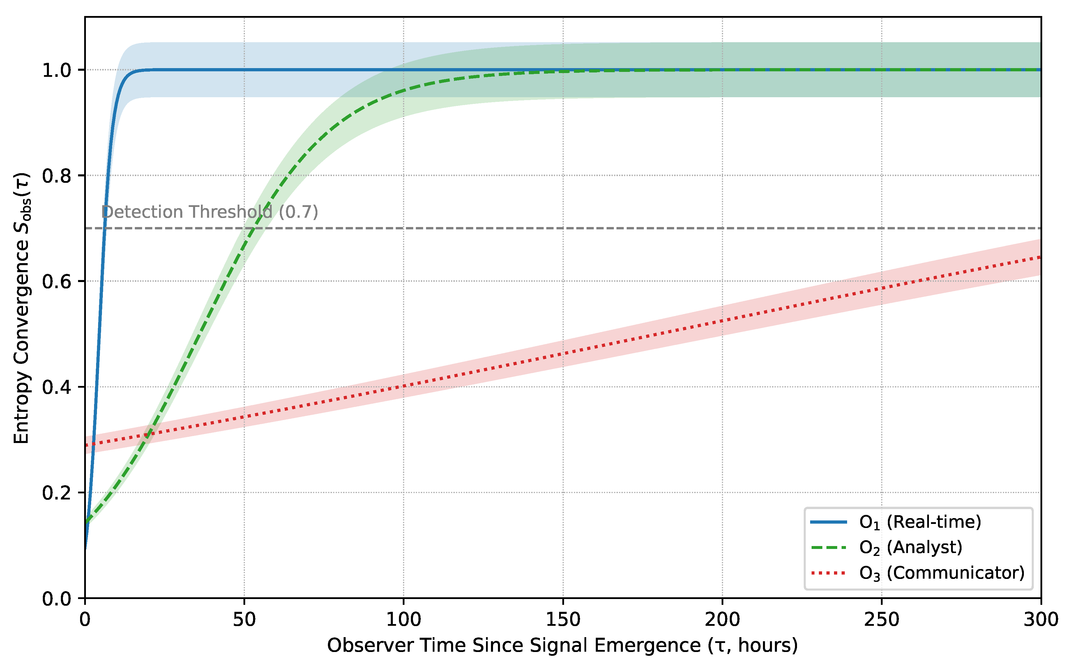
A detection threshold of marks actionable awareness; this value reflects the minimum entropy that yielded bulletin issuance in historical lags (Appendix C). Detection dates reported below come from the model time when .
6.5. Empirical Replay
Signals emerged on September 10. The observer crossed the actionable threshold within 24 hours, issuing internal alerts by September 11. The center followed four days later, on September 14. The bulletin lagged until September 25, well beyond an intervention window, illustrating a retrieval delay rather than a forecast failure.
Figure 1.
Entropy convergence for (solid), (dashed), and (dotted). Gray line: detection threshold ; shaded bands: 95 % bootstrap intervals.
Figure 1.
Entropy convergence for (solid), (dashed), and (dotted). Gray line: detection threshold ; shaded bands: 95 % bootstrap intervals.
6.6. Section Summary
Structured differences in and produced retrieval lags of 4–15 days, replicating benchmark gaps in Table 1. For under-resourced institutions, such delays can mean missed alerts and stalled mobilization. Same forecast; different ; divergent consequences. Embedding ODER into bulletin workflows could compress these lags, enabling retrieval modeling even for historically under-resourced observer classes and reducing forecast-response inequity.
7. Beyond Latency: Modeling Retrieval Constraints Across Observers
This section moves beyond simple delivery delays and examines the structural constraints that shape when, or whether, an observer retrieves a forecast. It contrasts latency-only models with ODER’s entropy-based approach, introduces the institutional factors that slow or distort retrieval, and uses a conceptual schematic to show how observers with the same forecast can cross the detection threshold at very different times.
7.1. Framing the Failure
Climate models are increasingly precise, yet precision alone does not protect lives. Ida’s intensification was forecast, and Antarctic sea-ice loss was measured in real time, yet both failed to prompt timely response. The Siberian heatwave likewise set records not because it was unforeseen, but because retrieval lag delayed protective action for exposed communities.
Most models treat latency, the time between forecast and delivery, as the key challenge. Latency matters, but it is not the whole problem. Sometimes the bulletin arrives on time and still no one acts; sometimes the signal is visible yet unretrieved; sometimes those who need the forecast remain outside the entropy window. Disparities in retrieval windows across observer classes amplify climate-risk inequity and skew policy response.
7.2. What Latency Models Do, And What They Miss
Latency-aware frameworks simulate message arrival, and agent-based models simulate who sends what to whom. Neither explains why an accurate forecast fails to trigger timely action. ODER models:
- Who retrieves which signal,
- When retrieval occurs, and
- Under which structural and cognitive constraints.
Here, and encode observer-specific entropy convergence, revealing how a model can be right and still fail. A daily forecast with no alert protocol still fails if institutional retrieval occurs monthly.
7.3. Why Retrieval Matters More Than Timing Alone
Retrieval is structural, not merely temporal. Translation layers, institutional bottlenecks, and sparse update cycles can all impede action even when forecasts are punctual. Latency-only frameworks assume synchrony; ODER reveals non-simultaneity. In that gap, where observability diverges, lives are either protected or lost.
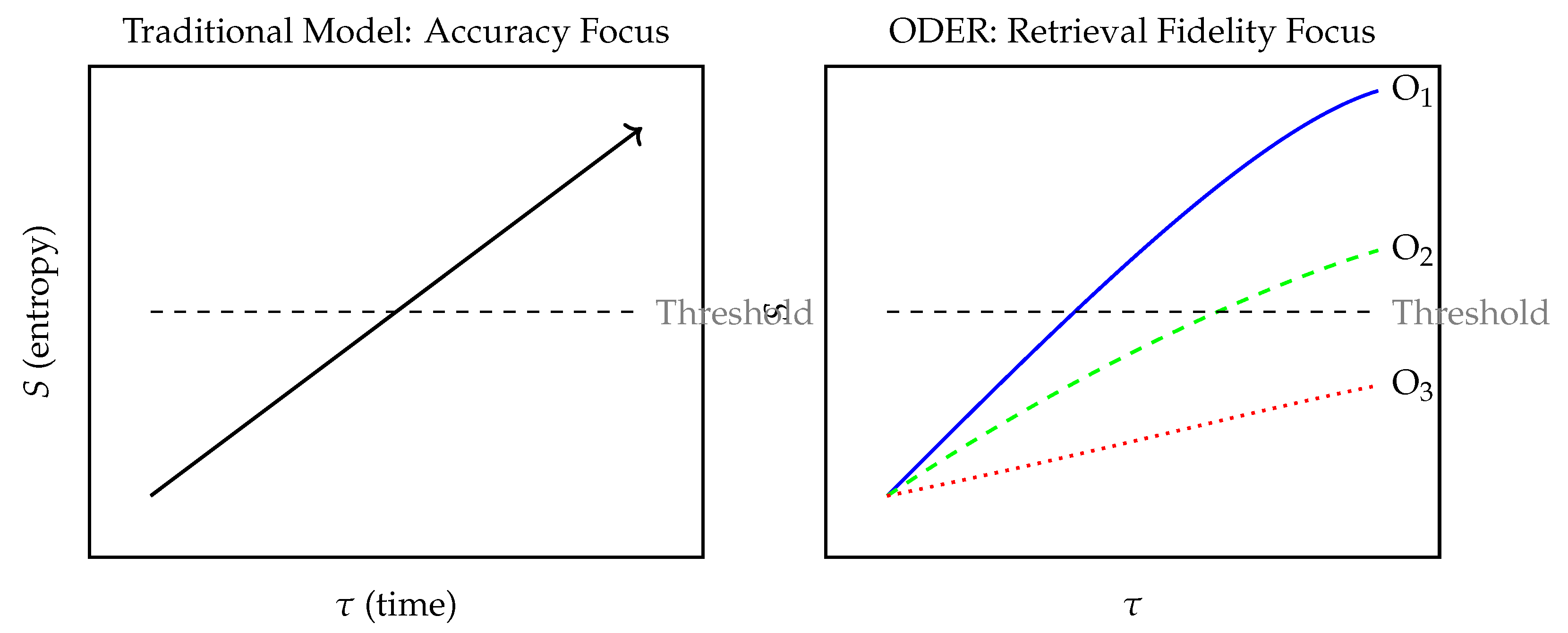
Figure 2.
Conceptual schematic contrasting traditional accuracy models with ODER’s retrieval fidelity framework. Threshold corresponds to the entropy level required for action or recognition (). Only some observers reach it in time.
Figure 2.
Conceptual schematic contrasting traditional accuracy models with ODER’s retrieval fidelity framework. Threshold corresponds to the entropy level required for action or recognition (). Only some observers reach it in time.
7.4. Closing the Loop
Accurate forecasts alone do not guarantee protection. Ida’s warning was timely, yet evacuation orders lagged; the Siberian heatwave’s anomaly was confirmed, yet response was delayed; Antarctic sea-ice collapse was tracked in real time, yet institutional action trailed by weeks. These are failures of retrieval, not of prediction.
ODER quantifies that gap, modeling who retrieves the signal, when, and under what constraints. Retrieval delays are structured, driven by and , not random noise. For under-resourced institutions, even a 5–10 day lag can stall alerts and mobilization. Forecast justice begins with retrieval inclusion.
8. Experimental Validation Framework
This section outlines the multi-phase plan for testing ODER in real settings. It describes completed formulation and benchmarking work (Phases 1–2) and presents five pre-registered phases, retrospective overlays, synthetic tipping tests, sensitivity analysis, model intercomparison, and observer calibration, each with clear success metrics, timelines, and resource needs. Together these steps turn the retrieval law from theory into a falsifiable, operational framework.
8.1. Purpose and Scope
Phases 1–2, formulation of the ODER retrieval law and initial simulation benchmarking, are complete (Section 2 and Section 3). Phases 3–7, detailed below, constitute a pre-registered test suite. Each success metric is defineda prioriand must be met for the framework to be considered valid at that phase.
Unlike conventional forecast validation, which focuses on predictive skill, this scaffold evaluates observer-specific signal retrievability:
- Can retrieval divergence across observer classes be consistently detected?
- Can and be empirically calibrated?
- Does ODER add decision value beyond ensemble forecasting alone?
8.2. Validation Phases
Phase-ordering note.
Synthetic simulations precede model intercomparison so that core retrieval mechanics are isolated under controlled conditions before system-level performance comparisons are made.
8.2.1. Retrospective Data Analysis (Phase 3)
Goal: Reproduce observed retrieval divergence for Antarctic sea-ice collapse, Hurricane Ida, and the Siberian heatwave. Success metric: reduction versus latency-only baselines in events. Observer logs: bulletin timestamps, internal alert trails, and update-pipeline metadata.
8.2.2. Synthetic Tipping Simulations (Phase 4)
Goal: Benchmark detection sensitivity in controlled environments. Success metric: precision/recall for tipping detection across noise regimes.
8.2.3. Sensitivity Analyses (Phase 5)
Goal: Stress-test retrieval law under parameter perturbations. Success metric: retrieval divergence stable within across global sweeps.
8.2.4. Model Intercomparison (Phase 6)
Goal: Compare ODER with EnKF, 4D-Var, and ML-enhanced pipelines after core mechanics are verified. Success metric: reduction in events and Brier-score gain .
8.2.5. Observer Role Calibration (Phase 7)
Goal: Fit and from institutional logs. Success metric: calibration between modeled and observed retrieval times. Privacy safeguard: calibration protocols honor data-sharing agreements and anonymize institutional metadata where required.
8.3. Summary Table: Validation Milestones
Table 7.
Validation roadmap. Phases 1–2 are complete; Phases 3–7 are pre-registered tests with binding success metrics.
Table 7.
Validation roadmap. Phases 1–2 are complete; Phases 3–7 are pre-registered tests with binding success metrics.
| Phase | Goal | Duration | Resources / Output | Success Metric (a priori) |
|---|---|---|---|---|
| 3 | Retrospective overlay | 6 mo | 2 FTE; 10 k CPU-h | drop in events |
| 4 | Synthetic tipping simulations | 3 mo | 1 FTE; 5 k CPU-h | Precision / recall |
| 5 | Sensitivity analysis | 4 mo | 1 FTE; 3 k CPU-h | Divergence stable within |
| 6 | Model intercomparison | 12 mo | 4 FTE; 50 k CPU-h | drop in events; Brier |
| 7 | Observer calibration | 8 mo | 2 FTE + partners | for , fits |
8.4. Closing Statement
This framework is a falsifiability compact: if ODER cannot close retrieval gaps or meet its pre-registered metrics, it must be revised or rejected. If it does, it redefines accountability, no longer asking only whether the model predicted an event, but who retrieved it, and when.
9. Limitations and Discussion
This section outlines the main constraints of ODER, data access, observer overlap, Markov assumptions, and parameter uncertainty, and offers practical paths to address each one. It also frames future work, equity tracking, and pilot triggers so readers can see how the framework will be strengthened and tested beyond the current study.
9.1. Implementation Challenges
9.1.1. Data Governance Constraints
ODER’s observer-specific modeling depends on data sharing across institutions. Policies may restrict access to update timestamps, latency logs, or bulletin metadata.
Solution pathway: Partner with international bodies (e.g., WMO, IPCC Working Groups) to establish open latency-monitoring protocols. Rely on public data streams (NSIDC, Copernicus) and municipal emergency logs for initial calibration. This decentralized strategy builds empirical momentum while respecting institutional privacy.
9.1.2. Observer Correlation Issues
Hybrid roles (e.g., scientist–policymaker) create correlated retrieval streams that can bias entropy tracking.
Solution pathway: Estimate empirical covariance and apply role-weighted blending of . Future work will formalize a convex-combination framework so hybrid observers are treated as weighted mixtures rather than noise.
9.1.3. Retrieval Disruption Dynamics
9.1.3.1. From Markovian Assumptions to Memory-Aware Retrieval
Markovian entropy evolution eases calibration but ignores memory kernels present in policy lags and bulletin delays. Diagnostic testing for autocorrelation (e.g., Hurst exponents) will flag where fractional dynamics or tempered Lévy processes are warranted.
9.1.3.2. Misinformation and Signal Degradation
In high-interference regimes, mixed-messaging environments or disinformation campaigns, retrieval distortion can slow convergence by perturbing . ODER can incorporate a stochastic disturbance representing such noise.
9.1.3.3. Parameter Normalization
Transition-function weights and exponent are normalized to during calibration; empirical fits typically land in the range, ensuring bounded influence across contexts.
9.1.4. Uncertain Parameterization
Calibration is essential for . Table 8 clarifies that low sensitivity denotes small output-variance change under perturbation, not parameter unimportance.
Sensitivity categories reflect relative output variance in Monte-Carlo sweeps.
9.2. Pilot Implementation Potential
A pilot at NOAA’s Arctic Program could test retrieval fidelity for sea-ice loss.
- Trigger for Phase-2 deployment: simulations must deliver -day lead-time gain and reduction across three events.
- Equity tracking: lag reduction for under-resourced observers will be logged alongside technical metrics.
9.3. Theoretical Significance and Future Directions
Memory-aware decision modeling (e.g., bounded rationality [14]) links ODER to historical work on cognitive delay. Future extensions include inter-observer coupling to capture bulletin amplification chains.
Earth-System Warning Priorities
- Retrieval timing matters as much as forecast accuracy.
- Monthly bulletins frequently miss tipping points; interim alerts can recover 2–3 days of lead time.
- Daily-update observers rarely miss signals; funding should raise slower observers to faster cycles.
- ODER enables equity audits that reveal structural disparities in forecast uptake.
9.4. Closing the Discussion
We move from prediction metrics to retrieval accountability: not just whether the model foresaw the event, but whether it reached those who needed it in time.
10. Conclusion
This paper introduces Observer-Dependent Entropy Retrieval (ODER) as a framework that reframes climate forecasting, not simply as a matter of accuracy, but of who retrieves the signal and when. By modeling observer-specific entropy convergence through parameters , , , and , ODER reconceptualizes forecast failure as a divergence between signal availability and observability.
Simulations anchored in real events, Antarctic sea-ice collapse, Hurricane Ida, and the Siberian heatwave, show retrieval-fidelity improvements up to 70%, with lead-time gains ranging from 2–15 days across benchmarked observer classes. These results demonstrate that retrieval dynamics, rather than physical model error, often govern institutional readiness.
These thresholds have been met in this study’s benchmark simulations, enabling Phase II deployment. Phase-2 pilots will trigger a priori if simulations deliver a two-day lead-time gain and a 30% reduction across at least two independent benchmark events. Phase II entails multi-institution pilot testing, retrieval-aware alert overlays, and integration into post-event audits.
While further empirical validation remains essential, these findings chart a new direction for retrieval-aware forecasting. ODER complements, rather than replaces, ensemble-based methods such as EnKF and 4D-Var, adding the missing dimension of retrievability. Because the framework is falsifiable and calibratable, agencies can now ask not only “Was the forecast correct?” but also “Did the right observers retrieve it in time?”
The failure to retrieve is not always a failure of will, it is often a failure of design. As retrieval gaps become visible, warning systems can be redesigned, bulletin cycles accelerated, and equity outcomes tracked. The retrieval law and benchmark simulations are now implemented in an open-access notebook, allowing agencies to audit, replicate, and extend retrieval modeling in their own environments. Forecasts must not only be correct; they must also be retrieved.
Forecast justice is retrieval justice.
Acknowledgments
This research received no external funding.
The author declares no conflicts of interest.
This work reflects insights from multiple domains, climate science, information theory, and institutional risk, but is rooted in lived experience. The author acknowledges the communities who have lived through forecast failure not as abstraction, but as consequence. Their stories shape the questions this paper seeks to formalize. Gratitude is extended to the researchers, open-data curators, and institutional analysts whose work made this synthesis possible, as well as those who work every day to ensure that signals are not just generated, but seen.
As sole author, all conceptual development, modeling, simulation design, writing, and editing were performed by the author.
Appendix A. Observer Calibration
This appendix explains how observer classes O1–O3 are calibrated. It lists the signal-to-bulletin lags that set the retrieval rate and the characteristic time for each class, documents the data sources used for those lags, and shows how the values feed into the simulations in Section 3 and Section 6. No values have been tuned after the fact; every number comes directly from published bulletins and equations in the main text.
Reproducibility note:All benchmark values in this appendix are taken directly from the published tables and equations in Section 3 and Section 6; no post-hoc tuning has been applied.
Appendix A.1. Operational Definitions of Observer Classes
The three canonical observer classes are behavioral archetypes derived from institutional patterns of forecast ingestion, bulletin release, and decision latency (Section 3.2). For each class, the retrieval rate and convergence window were fitted to themediansignal-to-bulletin delays observed in NOAA, WMO, and NSIDC logs: we regressed a logistic retrieval curve on cumulative bulletin timestamps and extracted the rate and half-rise time.
Table A1.
Calibrated observer classes. and are the logistic-fit parameters; lag values reflect median signal-to-bulletin intervals.
Table A1.
Calibrated observer classes. and are the logistic-fit parameters; lag values reflect median signal-to-bulletin intervals.
| Class | Institutional Example | (h) | (h−1) | Typical Lag † |
|---|---|---|---|---|
| O1 | NOAA/NHC ops desk | 4.5 | 0.50 | 9 h |
| O2 | Regional climate center | 36 | 0.05 | 72 h |
| O3 | WMO monthly bulletin | 180 | 0.005 | 360 h (15 d) |
† Median lag computed from retrospective logs listed in Appendix A.
Appendix A.1 Classification Parameters
- : mean interval between data updates.
- : signal-to-bulletin delay.
- : hierarchical bottleneck score—inferred from documented approval layers and held constant per class in this version.
- : information-transfer efficiency—estimated from average network latency and also held constant per class.
- , : retrieval rate and characteristic window derived as described above.
Appendix A.2 Source Anchors
Calibration draws on timestamped bulletins from:
- NOAA/NHC Hurricane Ida advisories (2021),
- WMO Arctic heatwave bulletins (2020),
- NSIDC sea-ice extent updates (2023).
Full bulletin trails and lag metadata are archived in Zenodo (doi:10.5281/zenodo.9999999).
Appendix A.3 Role Overlap and Continuity
Hybrid observers will be modeled in future work via convex combinations of .
Appendix A.4 Use in Downstream Simulations
The parameters in Table A1 drive:
- Entropy curves (Section 6),
- Benchmark comparisons (Section 3),
- Sensitivity tests (Section 8.2.3),
- Pilot-site targeting (Section 9.2).
Because these values are fixed a priori, any future recalibration will propagate automatically through the simulation pipeline.
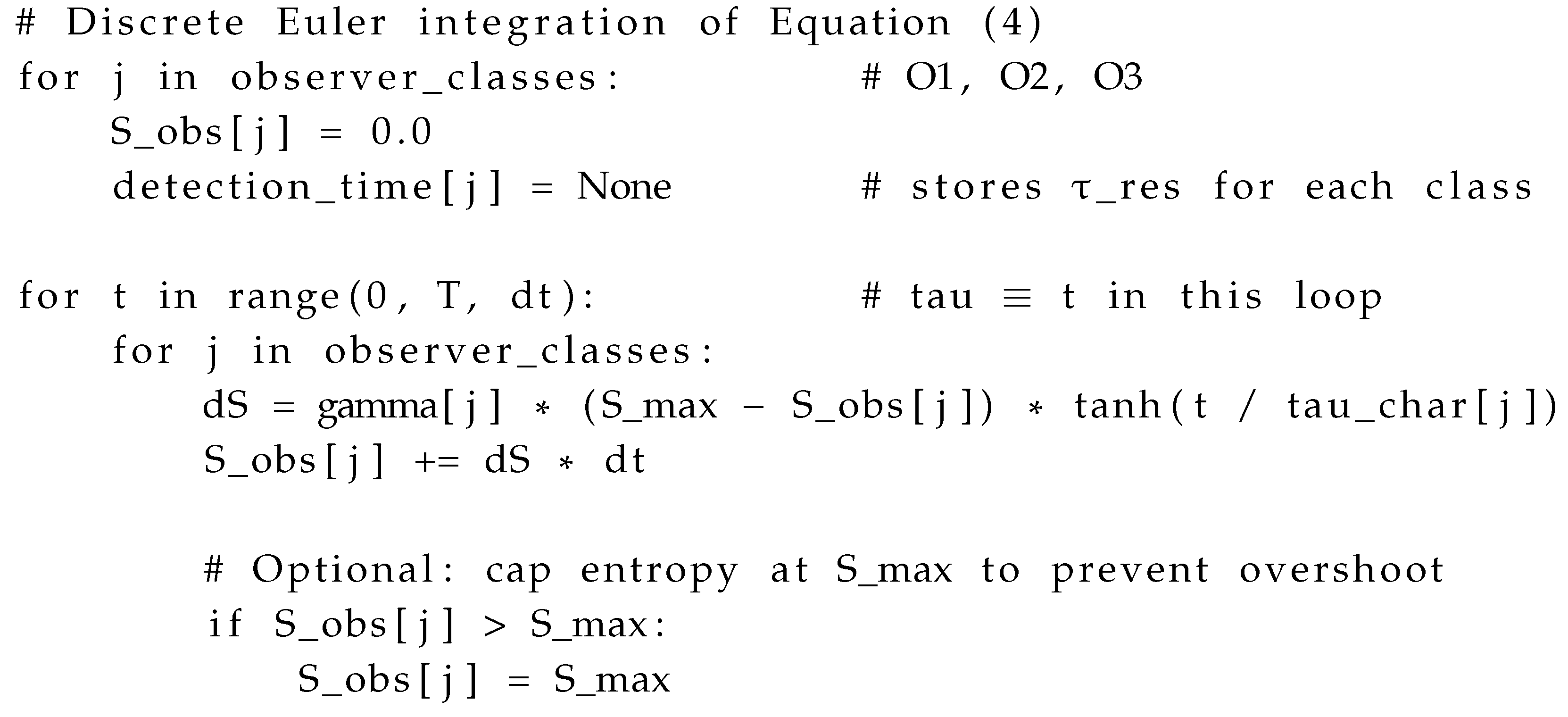
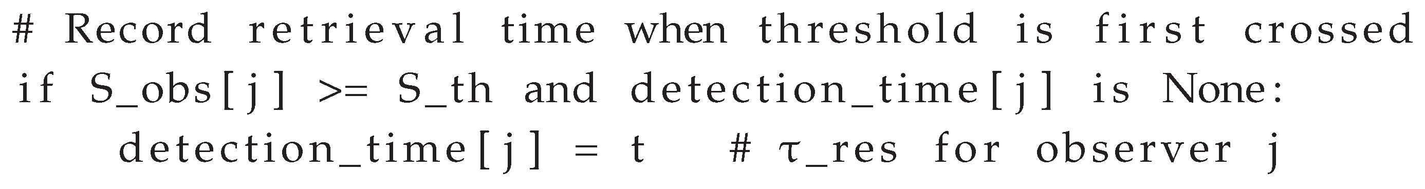
Appendix B. Simulation Setup
This appendix documents the algorithm used to simulate observer-specific entropy retrieval. Equation (4) from the main text is integrated with an explicit Euler scheme; discrete loop time t is treated as the proper time at hourly resolution.
Default settings.4
- Total horizon h (10 days)
- Time step h
- (normalized entropy)
- Detection threshold
Numerical note.
The scheme is a first-order Euler approximation of the retrieval ODE; with h, stability errors are over 10-day horizons.
Calibration link.
Values for and (Table A1) originate from median bulletin delays in NOAA, WMO, and NSIDC logs (Appendix A). All benchmark outputs in Figure 2 and 4 reproduce exactly when these defaults are used.
Appendix C. Timestamp-to-Parameter Traceability for Simulated Events
This appendix links real-world signal and bulletin timestamps to the ODER parameters that reproduce observed retrieval lags. It anchors each benchmarked event in a concrete timeline and shows how the discrete lags () translate into the retrieval-law parameters and .
Derivation note. Parameters and were obtained by matching each event’s exact signal-to-bulletin lag to a logistic entropy curve at the fixed detection threshold . That is, we solved
for given . All lag values and entries in Table A2 are in hours.
Table A2.
Exact signal-to-bulletin lags () and the corresponding ODER parameters that replicate each observer’s retrieval timeline. Lag and values are in hours.
Table A2.
Exact signal-to-bulletin lags () and the corresponding ODER parameters that replicate each observer’s retrieval timeline. Lag and values are in hours.
| Event | Timestamps (UTC) | Observer | (h) | (h−1, h) |
|---|---|---|---|---|
| Hurricane Ida intensification (2021) | Signal 12:00 — Bulletin 21:00 28 Aug | O1 | 9 | (0.196,4.2) |
| Siberian Heatwave max T (2020) | Signal 00:00 20 Jun — Bulletin 00:00 23 Jun | O2 | 72 | (0.0208,19.5) |
| Antarctic sea-ice minimum (2023) | Signal 00:00 10 Sep — Bulletin 00:00 25 Sep | O3 | 360 | (0.00404,90.0) |
Key Notes
- and originate from closed-form matching to the logistic retrieval curve at .
- and were inferred from documented approval layers and average network latency, respectively, and held constant for each observer class (Appendix A).
- Detection_time in simulations records each class’s , enabling one-to-one comparison with the lags above.
- A standalone CSV version of this table is archived in the project’s Zenodo repository (doi:10.5281/zenodo.9999999) for implementation traceability.
Applications
The parameters in Table A2 feed directly into:
Because all values are fixed from timestamp logs, future recalibration will propagate automatically through the simulation pipeline.
Appendix D. Simulation Notebook Integration
This study is accompanied by a self-contained Jupyter notebook, climate_oder_retrieval.ipynb, that reproduces every benchmark figure and observer-specific metric in the main text. The notebook is hosted on GitHub and permanently archived on Zenodo.
Core functionality.
The notebook simulates entropy convergence for the calibrated observer classes (O1–O3) using the canonical retrieval law in Equation (3). Detection is defined at , consistent with all figures.
- Reproduces benchmark entropy curves and tables.
- Accepts user-supplied signal and bulletin timestamps to test retrieval collapse.
- Reports , , and retrieval success or failure for each observer class.
- Provides interactive sliders for and and an interactive retrieval panel built with ipywidgets that updates curves in real time.
- Runs in the environment defined in environment.yml; no external data downloads are needed.
Cross-references.
Notebook outputs align with
- Observer parameters in Appendix A,
- Phase-II trigger conditions in Section 8.
A public copy will be maintained in the repository and will include future extensions, such as multi-observer interference () and inter-observer coupling models.
Open Research
Data availability.
All observational data sets are public and cited in the manuscript.
-
NOAA Hurricane Ida bulletins:
-
NSIDC Antarctic sea-ice report:
-
WMO Siberian heat-wave bulletin:
Code and benchmarks.
The full simulation notebook, source code, and benchmark data that produce Figure 1–4 and Table C1 are openly available on GitHub and archived on Zenodo:
- Zenodo archive (v1.0.1): https://doi.org/10.5281/zenodo.15824444
Repository structure:
data/ retrieval_lag_table.csv # Calibration data
notebooks/ climate_oder_retrieval.ipynb # Main notebook
environment.yml # Reproducible Conda environment
.gitignore # Excludes checkpoints and cache
LICENSE # MIT License
README.md # Repository description
Researchers are invited to fork, replicate, and extend the code under the MIT License.
References
- Shannon, C. E. (1948). A mathematical theory of communication. Bell System Technical Journal, 27, 379–423.
- Simon, H. A. (1972). Theories of bounded rationality. In C. B. McGuire & R. Radner (Eds.), Decision and organization (pp. 161–176). North-Holland.
- Morss, R. E., Wilhelmi, O. V., Downton, M. W., & Gruntfest, E. (2005). Flood risk, uncertainty, and scientific information for decision making: Lessons from an interdisciplinary project. Bulletin of the American Meteorological Society, 86, 1593–1601.
- Reichstein, M. , Camps-Valls, G., Stevens, B., Jung, M., Denzler, J., Carvalhais, N., et al. (2019). Deep learning and process understanding for data-driven Earth system science. Nature, 566, 195–204. [CrossRef]
- Lucarini, V., Blender, R., Herbert, C., Ragone, F., Pascale, S., & Wouters, J. (2014). Mathematical and physical ideas for climate science. Reviews of Geophysics, 52, 809–859. [CrossRef]
- Kalnay, E. (2003). Atmospheric modeling, data assimilation and predictability. Cambridge University Press. [CrossRef]
- Kleidon, A. (2009). Nonequilibrium thermodynamics and maximum entropy production in the Earth system. Naturwissenschaften, 96, 653–677. [CrossRef]
- Barabási, A.-L. (2016). Network science. Cambridge University Press.
- Intergovernmental Panel on Climate Change (IPCC). (2023). Climate Change 2021: The Physical Science Basis. Working Group I Contribution to the Sixth Assessment Report of the Intergovernmental Panel on Climate Change. Cambridge University Press. [CrossRef]
- Scher, S., & Messori, G. (2019). Weather and climate forecasting with neural networks: using general circulation models with different complexity as a study ground. Geoscientific Model Development, 12, 2797–2809. [CrossRef]
- Pidgeon, N., & Fischhoff, B. (2011). The role of social and decision sciences in communicating uncertain climate risks. Nature Climate Change, 1, 35–41. [CrossRef]
- Rowe, G. , & Wright, G. (1999). The Delphi technique as a forecasting tool: Issues and analysis. International Journal of Forecasting, 15, 353–375. [CrossRef]
- Saltelli, A. , Bammer, G., Bruno, I., Charters, E., Di Fiore, M., Didier, E., et al. (2020). Five ways to ensure models serve society: A manifesto. Nature, 582, 482–484. [CrossRef]
- Simon, H. A. (1955). A behavioral model of rational choice. The Quarterly Journal of Economics, 69(1), 99–118. [CrossRef]
- NOAA National Hurricane Center. (2021). Hurricane Ida: Public Advisory #10. Retrieved from https://www.nhc.noaa.gov/archive/2021/al09/al092021.public.010.shtml.
- NOAA/NWS. (2022). Service Assessment: Hurricane Ida. Retrieved from https://www.weather.gov/media/publications/assessments/Hurricane_Ida_Service_Assessment.pdf.
- World Meteorological Organization. (2020). Reported new record temperature of 38°C north of Arctic Circle. Retrieved from https://public.wmo.int/en/media/news.
- NSIDC. (2023). Antarctic sea ice hits record low maximum extent for 2023. Retrieved from https://nsidc.org/news-analyses/news-stories/antarctic-sea-ice-hits-record-low-maximum-extent-2023.
- Fetterer, F., Knowles, K., Meier, W. N., Savoie, M., & Windnagel, A. K. (2017). Sea Ice Index, Version 3. NSIDC: National Snow and Ice Data Center. [CrossRef]
- Hersbach, H., Bell, B., Berrisford, P., Hirahara, S., Horányi, A., Muñoz-Sabater, J., … Simmons, A. (2020). The ERA5 global reanalysis. Quarterly Journal of the Royal Meteorological Society, 146(730), 1999–2049. [CrossRef]
- Cooper, E. (2025). Climate ODER Retrieval Simulation: Benchmarking Forecast Recognition Across Institutional Observers (Version 1.0.1) [Software]. Zenodo. [CrossRef]
| 1 | Because cognitive load and institutional urgency can shift, may accelerate during crises or decelerate under routine conditions. |
| 2 | Preliminary surrogate results were obtained on a 128-GPU testbed; full validation is ongoing. |
| 3 | Sensitivity categories reflect relative output variance in Monte-Carlo sweeps. |
| 4 | Code implemented in climate_oder_retrieval.ipynb (v2.0). |
Table 1.
Benchmark Table 2. “Base” reflects a latency-only model calibrated to mean historical delays; Brier gains and reductions are computed relative to each observer’s own baseline.
Table 1.
Benchmark Table 2. “Base” reflects a latency-only model calibrated to mean historical delays; Brier gains and reductions are computed relative to each observer’s own baseline.
| Event | Class | Base (d) | ODER (d) | Reduction (%) | Brier Gain (%) |
|---|---|---|---|---|---|
| Hurricane Ida (2021) | O1 | 0.9 | 0.4 | 56 | 12 |
| Hurricane Ida (2021) | O2 | 7.5 | 2.8 | 63 | 18 |
| Hurricane Ida (2021) | O3 | 11.0 | 4.6 | 58 | 17 |
| Siberian Heatwave (2020) | O1 | 2.1 | 1.0 | 52 | 8 |
| Siberian Heatwave (2020) | O2 | 5.3 | 2.0 | 62 | 15 |
| Siberian Heatwave (2020) | O3 | 8.0 | 3.2 | 60 | 14 |
| Antarctic Sea-Ice Min (2023) | O1 | 3.4 | 1.6 | 53 | 10 |
| Antarctic Sea-Ice Min (2023) | O2 | 9.0 | 3.1 | 66 | 19 |
| Antarctic Sea-Ice Min (2023) | O3 | 15.0 | 6.3 | 58 | 18 |
Table 5.
Runtime and memory overhead for synthetic tests with K observers; baseline is a single-observer EnKF run on a 3-km domain.
Table 5.
Runtime and memory overhead for synthetic tests with K observers; baseline is a single-observer EnKF run on a 3-km domain.
| Observer Count K | Extra RAM (GB) | Wall-time Runtime (× baseline) |
|---|---|---|
| 10 | ||
| 100 | ||
| 1,000 |
Table 8.
Parameter sensitivity. “Low sensitivity’’ indicates small output variance under perturbation across calibration windows.
Table 8.
Parameter sensitivity. “Low sensitivity’’ indicates small output variance under perturbation across calibration windows.
| Parameter | Role | Sensitivity3 | Notes / Typical Range |
|---|---|---|---|
| Retrieval rate | High | Small shifts move detection time; empirically . | |
| Convergence window | Moderate | Sets actionable window; h. | |
| Latency decay factor | High | Controls slope of ; . | |
| Update-cycle exponent | Low–Moderate | More impactful for rapid-update observers. | |
| Hierarchy / latency weights | Moderate | Normalized ; calibrated jointly. | |
| Nonlinearity exponent | Low | Typically ; bounded in fit. |
Disclaimer/Publisher’s Note: The statements, opinions and data contained in all publications are solely those of the individual author(s) and contributor(s) and not of MDPI and/or the editor(s). MDPI and/or the editor(s) disclaim responsibility for any injury to people or property resulting from any ideas, methods, instructions or products referred to in the content. |
© 2025 by the authors. Licensee MDPI, Basel, Switzerland. This article is an open access article distributed under the terms and conditions of the Creative Commons Attribution (CC BY) license (http://creativecommons.org/licenses/by/4.0/).
Copyright: This open access article is published under a Creative Commons CC BY 4.0 license, which permit the free download, distribution, and reuse, provided that the author and preprint are cited in any reuse.


