A Receptor Model and CTM Integrated PM_2.5 Source Apportionment Approach and Its Application in 2+26 Cities Region of China

1. Background

PM_2.5 components include primary components, which are directly emitted from emission sources, and secondary components, such as sulfate, nitrate and secondary organic aerosol (SOA), which are converted from certain primary air pollutants or precursors such as SO₂, NOx and volatile organic compounds (VOCs) in atmospheric chemical reactions. The relationships between PM_2.5 secondary component concentrations and their contributing emission sources are complex, usually non-linear and not even always positive due to the complex chemical reactions and other atmospheric processes. The methodology of PM_2.5 source apportionment can be complex due to the intricate chemical transformation, transport, and removal processes involved. To develop effective policies and action plans, it is crucial to identify the sources of PM_2.5 and understand their contributions. The process to identify or resolve the contribution of emission sources to the concentration of PM_2.5 at specific locations for a certain period is PM_2.5 source apportionment.

In North America and Europe, extensive source apportionment studies have been conducted to quantitatively identify the contribution of emission sources to particulate air pollution (Viana, M., et al., 2008; Belis et al., 2012; Hopke P. K., 2016; Belis et al., 2019). PM Source apportionment research in China started in the late 1980s, and there were only a few research conducted in the 1980s and 1990s (Liang J., & Wang W., 1990; Dai, et al., 1995). Since 2000, especially in the current decade, the source apportionment work on particulate matter using different modeling methodologies in China has been experiencing explosive growth (Tian et al., 2016; Wang, J., 2016; Z. Zhang et al., 2017; Zhao, P., et al., 2013; Zhao, X., et al., 2013; Wang, D. et al., 2020). However, different modeling approaches possess distinct advantages, limitations, and inherent uncertainties.

2. Integrated PM_2.5 Source Apportionment Modeling Approach

In general, there are two major categories of models for PM_2.5 source apportionment: receptor models and air quality models.

2.1. Receptor Models

The PM_2.5 components measurement data, such as SO₄^2-, NO₃^-, NH₄⁺, EC, OC and elements, can provide only limited information about the contribution of emission sources and atmospheric physical and chemical processes. Receptor models are frequently employed to further quantitatively resolve the contribution of PM_2.5 sources. Using statistical methods, receptor models estimate or resolve the contributions of emission sources based on PM_2.5 components concentration data and PM_2.5 composition profiles of the contributing emission sources, either explicit or implicit. The receptor models are based on the principle of mass balance, assuming that the relationship between PM_2.5 concentrations and their sources are linear, and the measured concentrations of PM_2.5 components at a specific receptor site are the sum of the contribution of corresponding components of emission sources (Hopke P. K. 2016). In theory, receptor models can quantitatively identify the contributions to primary PM_2.5 of all contributing emission sources without being constrained by the information and data of emission inventories and the atmospheric processes involved.

Based on different assumptions and input data requirements, there are many different receptor models. The CMB model is one of the most used mass balance receptor models developed by many authors and developed into the software of the U.S. EPA (Watson et al., 1991). CMB model assumes that the contributing sources or sources categories are known and the chemical composition profile (fingerprints) of the source/source categories are available (explicit). The drawback of this assumption is that the resolved sources/source categories are pre-decided, and the unknown contributing sources would be missed. The other most used receptor model is Positive Matrix Factorization (PMF) (Paatero & Tapper, 1994; Paatero, 1997a), which can resolve the contributing sources without the prerequisite of known or explicit source composition profiles. However, the results of PMF are more easily affected by the uncertainties in the measured PM components data and the source apportionment results also need source composition profiles as reference. In this work, we used the CMB model results from the Project of PM_2.5 Source Apportionment in the 2+26 Cities for 2+26 (MEE, 2020).

The basic assumptions of CMB model are (Watson, 2004): 1) compositions of emission sources (source categories in most cases) are known and constant over the period of ambient and source sampling; 2) chemical species do not react with each other and are independent of each other during transport, i.e., the relationship between the contribution of components of PM_2.5 from one source at a receptor, is linear to the component profile of that sources; 3) all sources with potential for contributing to the receptor have been identified; and 4) measurement uncertainties are random, uncorrelated, and normally distributed. 5) the number of source categories is less than or equal to the number of the PM_2.5 components . If the above assumptions are satisfied, the following theoretical form of the CMB model is valid:

$$c_{ij}={\sum }_{k=1}^{k_0}{g_{jk}f}_{ik}+e_{ij}$$

(1)

where $c_{ij}$ is the concentration of chemical species i measured in the sample j of interest, g_jk is the contribution of source category k to sample j, f_ik is the concentration of chemical species i (chemical components profile) in the PM_2.5 emission source category k, e_ik is the unmodeled portion of the variation.

If the number of source categories is less than or equal to the number of the PM_2.5 components, for each sample j, the best estimation of g_jk in the overdetermined equation system (1) can be found on a sample-by-sample basis by minimizing the error term using, for example, effective variance least squares (EVLS) in CMB model (U. S. EPA, 2004). The contribution of source sector k to the PM_2.5 concentration of j sample can also be calculated:

$${\tilde{c}}_{jk}={\sum }_{i=1}^{i0}{g_{jk}f}_{ik}$$

(2)

2.2. CTM Air Quality Models

The other PM_2.5 source apportionment method is to use air quality models. After decades of development, the air quality model has become very sophisticated. Air quality models can be broadly categorized based on their theoretical foundation and the spatial scale of their application. The Gaussian models describe the atmospheric turbulence diffusion and transport of wind of air pollutants and are suitable for simple terrain, simple chemical transformations and local scale air pollution problems. The other type of air quality model is the chemical transport model (CTM), which is based on a set of differential equations to simulate atmospheric chemical and physical processes, including the three-dimensional and time-varying advection transport of complicated wind fields, turbulence diffusion, chemical reactions in gaseous, aqueous, particulate and heterogenic phases, dry and wet removal processes of all relevant air pollutant species, and emissions from different sources. CTM models are good prediction tools for simulating the transport and chemistry of both primary and secondary air pollutants.

In the general form of chemical transport model (CTM), the concentration of species i at location (x,y,z) and time t, C_i(x,y,z,t) can be described as (Jacobson, 2005; Seinfeld & Pandis, 2006):

$${\displaystyle \frac{\partial C_i}{\partial t}}=-\mathit{u}·\nabla C_i+{\displaystyle \frac{1}{\rho }}\nabla \left(\mathsf{\rho }\mathit{K}\nabla C_i\right)+R_i+E_i+S_i$$

(3)

where C_i is the mixing ratio of species i, and the left term of equation (3) is the change rate of C_i over time. On the left side of equation (3), the first term is horizontal and vertical advection and u is the wind velocity; the second term is horizontal and vertical diffusion, where ρ is the air density, Κ is the diffusivity tensor; R_i is the chemical reaction including gas-phase chemistry, aqueous chemistry, aerosol dynamics and thermodynamics, which can be described by a set of ordinary differential equations of pollutants involved in the reactions and usually is non-linear; E_i is the emission rate; S_i is the scavenging term including the dry deposition and precipitation scavenging. In most CTM models, PM_2.5 components are simulated separately. The main PM_2.5 components include primary species such as crust species, BC, primary OC, primary sulfate, and secondary species such as sulfate, nitrate, ammonium, SOA. The PM_2.5 concentration is the sum of the concentration of the component. The CTMs are usually three-dimensional grid models, and the variables in equation (3) represent a grid or box. By integrating equation (3) over the entire simulation period and modeling domain, the concentrations of chemical species, including PM_2.5, can be obtained.

Based on different source apportionment methodologies, CTMs can estimate the contribution to PM_2.5 concentration of emission sources or source sectors with high spatial and temporal resolution. The commonly used methodologies include simulating different scenarios (Brutal Force) or using emission tracking methods such as PSAT in CAMx (Koo B., et al., 2009; Wagstrom, K. M., et al., 2008) and ISAM in CMAQ (Kwok et al., 2013).

Tagged source apportionment approach of CTM, track the contribution of targeted emission sources or source groups in the model simulation. The development of the tagged approach started from the primary emission source or the pollutants involving simple chemical reactions such as SO₂ and sulfate (Lane et al., 2007; McHenry et al., 1992). The accurate way is to track all the PM species back to the precursor gas species or primary component of all size bins of aerosol of targeted sources, which, nevertheless, is computationally demanding (Ying & Kleeman, 2006; Kleeman & Cass, 2001. Recent models such as the PSAT of CAMx and the TSSA of CMAQ (Wang, Z. S., et al., 2009) have employed a simplified tracking approach to chemistry and aerosol dynamics, making them more computationally efficient while still preserving accurate contribution information.

It is worth noting that E_i is only the emission source at the location or grid of (x,y,z) at time t. The concentration C_i is actually contributed by all emission sources over a sufficiently long period of time, both local（this grid） and non-local, due to the transport and transformation. The non-local emission sources could be even outside the modeling domain and beyond the modeling period, which are treated as boundary condition and initial condition of modeling.

By using tracking technology or the brute-force approach of CTM, C_i,k,n, the contribution to the concentration of species i of sector k of city n (a group of grids) can be calculated. The concentration of the component i of PM_2.5 at time t, (e.g., corresponding sample j) and a grid/site, C_i,bulk, can be described as:

$$C_{i,bulk}=C_{i,initial}+C_{i,boundary}+\sum _{n=1}^{n=n0}\sum _{k=1}^{k=k0}{C}_{i,k,n}$$

(4)

where n₀ is the total number of cities in the domain and k₀ is the total number of the source sectors; C_i,initial represents the contributions of the initial conditions of the simulation, which can be ignored if the simulation time is long enough; C_{i, boundary} represents the boundary conditions or the contributions from the sources outside the modeling domain; the third term of (4) and C_i,k,n represent the contributions from all source sectors of all cities in the modeling domain. The average concentration contribution ${\overline{C}}_{i,k,n}$ over a period of time, e.g. sampling time of one day, can also be obtained. In our approach, we do not directly use the concentrations simulated by the CTM model, thus avoiding the model uncertainty.

2.3. Integrated Source Apportionment Approach

Although the receptor model and the air quality model each specialize in their respective applicable situations, both the CTM model and the receptor model have theoretical and practical challenges and different sources of uncertainties. Firstly, the fundamental theoretical assumption of the receptor model is that the concentration of PM_2.5 at a certain point and time is the sum of contributions of possible emission sources, which is only valid for primary pollutants but not valid for secondary components of PM_2.5 due to the different speed or even non-linear chemical transformation. In CMB, the secondary components of sulfate, nitrate and SOA are treated as three independent sources (Watson, 2004a, 2004b; Hopke P. K., 2016). Secondly, the CMB model also could not resolve specific sources of same source sector, as well as the locations or administrative units, such as cities and provinces, of the contributing sources. Thirdly, the sources and components of raw materials and fuels often vary significantly, posing challenges in obtaining representative component profiles of emission sources and in interpreting source categories resolved by models such as PMF model. Finally, the CMB model can only identify a limited number of source or fuel categories, based on the number of the components and available PM_2.5 composition profiles.

On the other hand, there are few major sources of uncertainty for the CTM models. The first source of discrepancy is the gap between scientific mechanism or algorithms of models and the actual physical and chemical processes. For example, the uncertainties in simulating the formation of secondary PM_2.5 components, especially SOA, are still relatively high. Secondly, high uncertainties may exist in emission inventory including the emission amount, spatial and temporal resolution, as well as the composition or speciation profile of air pollutants especially for the primary organic matter, VOCs, and NOx. It is also difficult to obtain timely source emission data for crop residue burning, fugitive and wind-blown dust. The change of the emission sources due to economic development and control policy is another major source of uncertainty. This phenomenon was particularly pronounced in the 2+26 Cities Region during the period from 2017 to 2018. Thirdly, although the sampling points are set up to represent the city or region, they inevitably receive the impact of local emission sources such as fugitive and wind-blown dust, mobile emission, and other small random emission sources. Such kind of local contribution can be reflected by receptor models, but is often overlooked by CTM models due to resolution limitations and the level of detail and accuracy of emission inventories. Finally, due to the substantial computational resource requirements, the CTM model cannot conduct detailed source apportionment in a big area with a huge number of sources and too many source sectors, either using tracking technology or a brute-force approach (scenario analysis).

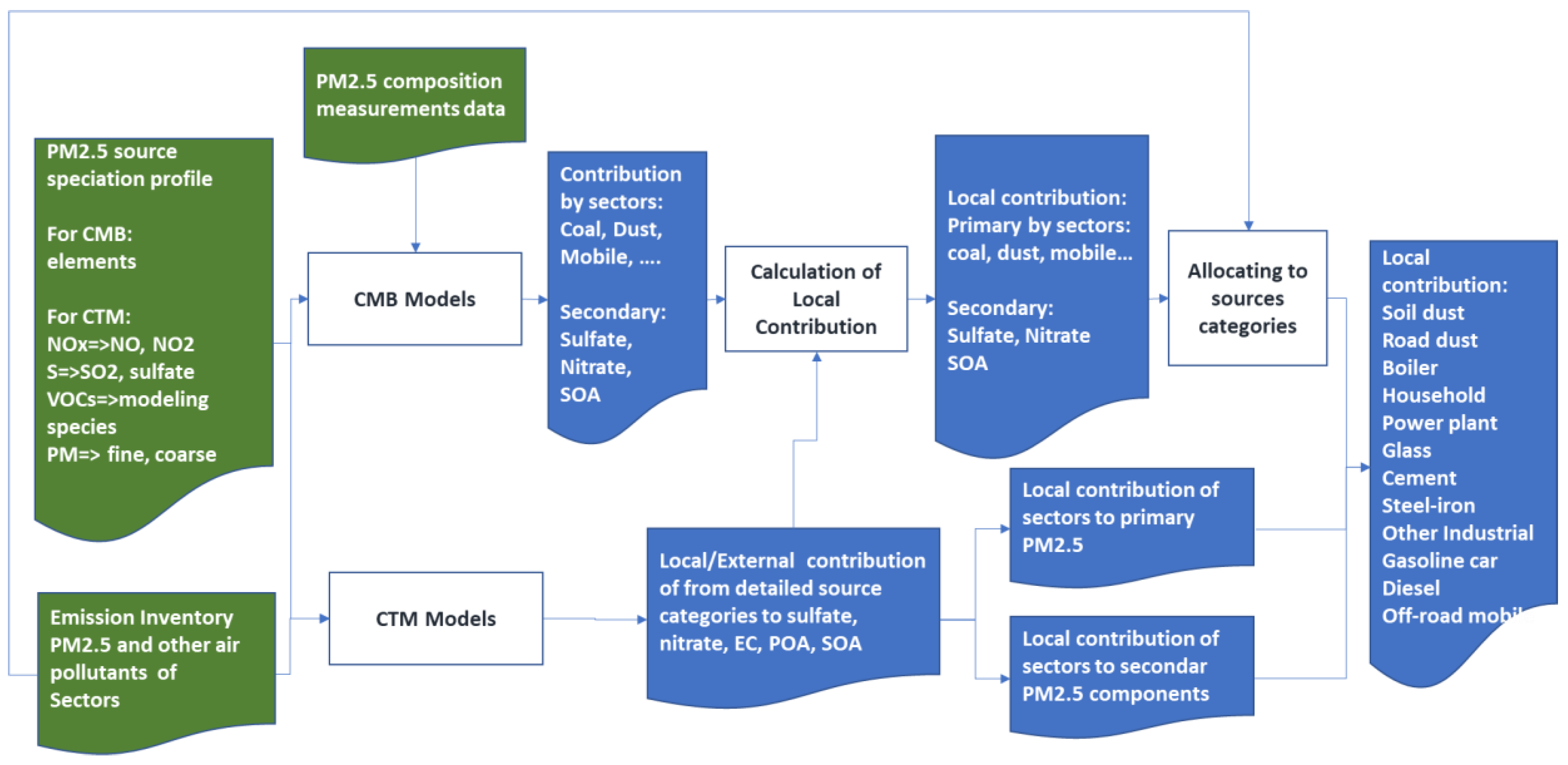
In this work, we developed an integrated approach, taking advantage of receptor models, chemical-transport model (CTM), PM_2.5 measurement data, and emission inventory. This approach obtains refined source apportionment results for each city through three steps: receptor modeling, air quality modeling, and integrated source apportionment (Fig.1). Firstly, we used the CMB receptor model and measured PM_2.5 component concentration to obtain the contributions of source sectors to the primary PM_2.5 or first-level source apportionment. In the second step, the air quality model was used to calculate the mutual contributions among cities of PM_2.5 components, including secondary components. Finally, combining the measured secondary portion of PM_2.5, the CMB source apportionment results for the primary PM_2.5, and the local and long-range transport contributions ratio of each component of PM_2.5 by CTM, the detailed local contribution of emission sectors or emission sources of each city were resolved.

This approach could take advantage of the relatively accurate PM_2.5 component measurement data, especially for secondary component, and the ability of receptor models to revolve the contributions of primary components based on the characteristics of emission sources. The approach also takes advantage of the ability to identify or track the contribution of specific emission sources in different locations or administration regions and the ability of CTM to simulate the long-range transport and non-linear transformation of secondary PM_2.5 components with high spatial and temporal resolution. Detailed information in the emission inventory, including accurate locations and composition profiles, can also be used in this approach to further resolve contributions at the local scale, where the linear relationship between source and concentration is applicable. This approach could overcome the difficulty of the receptor model in identifying the source of secondary components and resolving the specific emission sources and location, also overcome the uncertainty of CTM in emission inventory and high uncertainty in the simulation of secondary components such as sulfate and SOA.

Figure 1. Receptor model, CTM model, and emission inventory integrated source apportionment approach.

Figure 1. Receptor model, CTM model, and emission inventory integrated source apportionment approach.

For CTM source apportionment results, by summing up all the contributions by cities, we can obtain the contribution to PM_2.5 and its components from each sector or all sectors within that city. For city n’, the local contribution fraction to the concentration of species i and source sector k’ can be calculated:

$${\lambda }_{local,i,k^{\mathrm{\text{'}}},n^{\mathrm{\text{'}}}}={\displaystyle \frac{{\overline{C}}_{i,k^{\mathrm{\text{'}}},n^{\mathrm{\text{'}}}}}{\sum _{n=1}^{n=n0}{\overline{C}}_{i,k^{\mathrm{\text{'}}},n}}}$$

(5)

By applying this ratio to the source apportionment results of the CMB model (2), the local contribution of PM_2.5 concentration from source sector k in city n’ can be found:

$${\tilde{c}}_{local,j,k}={\lambda }_{local,i,k,n\mathrm{\text{'}}}{\tilde{c}}_{j,k}$$

(6)

It is worth noting that the sectors in CTM are more detailed than the one in CMB model, that is k’>k. The source apportionment results can also be obtained by applying CTM source apportionment results for the measured secondary components of PM_2.5 such as sulfate, nitrate and SOA, which can not be resolved by in CMB receptor model. Summing up all the components and averaging over the period of measurement time, in our case, the winter of 2017-2018, the PM_2.5 source apportionment of local contributions in one city can also be calculated.

3. The Application of the Integrated PM_2.5 Source Apportionment Approach in the 2+26 Cities Region

The 2+26 Cities Region includes Beijing, the capital of China, and Tianjin, the other direct-administered municipality of China, and other 26 large cities of Hebei Province, Henan Province, Shandong and Shanxi Province. Except for four cities of Shanxi Province, the most of 2+26 cities are located in the North China Plain. In general, the 2+26 cities are among the most densely populated and industrialized cities in China and have long experienced severe PM_2.5 air pollution. The cold temperatures of the cold and dry continental winter climate make heating essential. At the same time, frequent unfavorable stable meteorological conditions often lead to severe air pollution during the winter and autumn seasons.

Despite continuous improvements in air pollution in the 2+26 Cities Region, particularly with a rapid decrease in SO₂ levels, particulate air pollution especially the PM_2.5 pollution remained the most severe in the country. Throughout the winter of 2017–2018, the average PM_2.5 concentration in 28 cities ranged from 53.6 to 143.5 µg/m³, with an overall average of 95.4 µg/m³. This still significantly exceeded 35.0 µg/m³, the annual average limit of National Ambient Air Quality Standard of China (MEE, 2012) and the interim target 1 of the WHO Air Quality Guidelines (WHO,2021).

At the same time, the concentrations and contributing emission sources of PM_2.5 emissions in the region were also rapidly changing due to factors such as economic development, changes in energy consumption and structure, implementation of control policies and action plans, and variations in meteorology and atmospheric chemistry. Therefore, timely PM_2.5 source apportionment or the information on the contribution of PM_2.5 emission sources is important for the development and implementation of effective control policy and action plan.

To identify and estimate the contributions of emission sources, the integrated approach developed of this work was applied in the Project of PM_2.5 Source Apportionment in the 2+26 Cities during the autumn and winter of 2017-2018, which was a direct supporting activity to the Air Pollution Prevention and Control Action Plan (Action Plan) in 2013 (State Council of P. R. China, 2013, 2018).

3.1. Source Apportionment by CMB Receptor Model

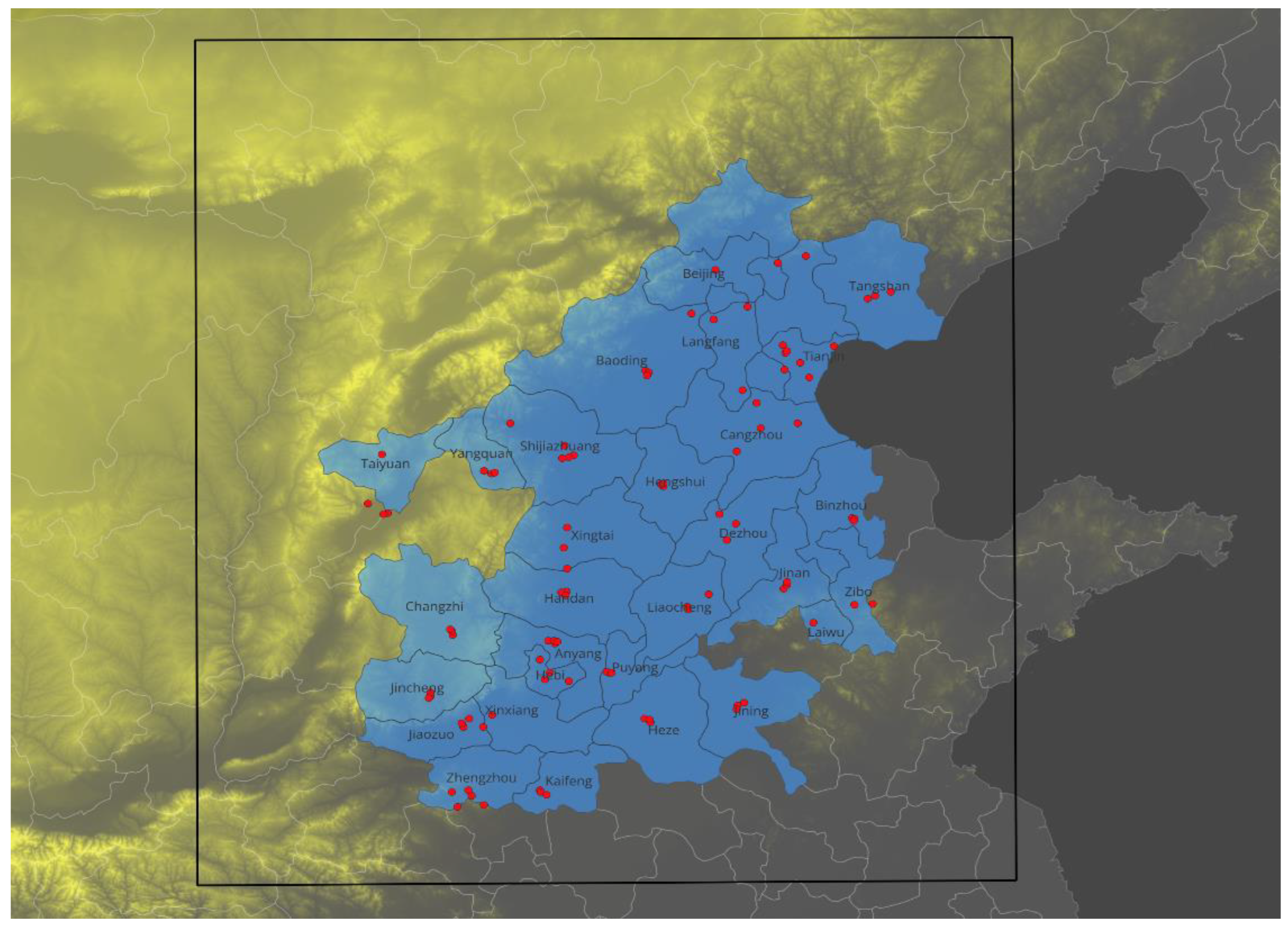
In this work, we used PM_2.5 components data measured in the Project of PM_2.5 Source Apportionment in the 2+26 Cities Region (MEE,2020). Although the information on the components of PM_2.5 cannot quantitatively provide complete information on the contribution of PM_2.5 sources, it can still provide valuable scientific information on the contribution of emission sources, and atmosphere physical and chemical processes. In this work, PM_2.5 component data of the 28 cities was obtained from the Project of PM_2.5 Source Apportionment in the 2+26 Cities Region in the Autumn and Winter of 2017-2018. A total of 109 sampling sites have been set up according to the representativeness and meteorological conditions. The sampling period for PM_2.5 was from October 15, 2017, to January 31, 2018. The daily averaged concentration of 35 chemical components including carbonaceous species (OC、EC), water-soluble inorganic ions (F^-, Cl^-, SO₄^2-, NO₃^-, Na⁺, K+, Ca²⁺, Mg²⁺, NH₄⁺) and at least 24 elements (Li, Be, Na, Mg, Al, Si, P, S, K, Ca, Sc, Ti, V, Cr, Mn, Fe, Co, Ni, Cu, Zn, As, Se, Sr, Ag, Cd, Sn, Sb, Ba, Hg, Ti, Pb) in PM_2.5 were obtained.

Figure 2. Beijing, Tianjin, and other 26 cities in the surrounding provinces region, the location of sampling sites and the modeling domain (only for illustrative purposes).

Figure 2. Beijing, Tianjin, and other 26 cities in the surrounding provinces region, the location of sampling sites and the modeling domain (only for illustrative purposes).

The data of PM_2.5 components can provide general information about the sources. In the 2+26 Cities Region, the composition of PM_2.5 changed notably as concentration levels changed. In the long-term trend, one of the significant changes is the increasing portion of organic matter (OM) as PM_2.5 concentration level decreased. The average concentration of organic components in the autumn and winter of 2017 among 28 cities was 22.4 µg/m³, accounting for 23.1% of PM_2.5 concentration. The increase of the organic matter proportion in PM_2.5 indicates that greater attention should be given to controlling automobile exhaust, biomass burning, in addition to coal combustion, as well as VOCs, which are precursors of SOA.

Secondary inorganic components, on the other hand, decreased but still contributed a significant portion of PM_2.5. Secondary inorganic components of particulate matter (PM) originate from atmospheric chemical reactions involving precursor gases such as sulfur dioxide and nitrogen oxides, which are closely related to the fossil fuel combustion such as coal and mobile sources, and ammonia (NH₃). With the rapid decrease in sulfate levels due to reduction of SO₂ emissions, nitrate emerged as the most significant inorganic secondary component of PM_2.5. Nitrate and sulfate had average concentrations of 16.5 µg/m³ and 10.2 µg/m³, respectively, contributing 17.8% and 10.7% to the total PM_2.5 concentration. The region was characterized by an ammonia-rich environment, with ammonium ion concentrations in PM_2.5 mainly influenced by the equilibrium of various anionic components, not by the emission of ammonia. The ammonium concentrations had an average concentration of 9.1 µg/m³, contributing 9.8% of PM_2.5 concentration.

Crustal elements typically originate from primary emission sources such as smoke, wind-blown dust and fugitive dust from human activities. In the 2017-2018 winter, the average contributions of crustal elements to PM_2.5 were 11.1 µg/m³ and contributed 11.4% in the 2+26 Cities Region. The crustal elements concentration varied significantly among cities, showing more local emission characteristics and meteorological conditions.

Element carbon (EC), resulting from incomplete combustion of fossil fuel, biofuel, and biomass, usually occurs under no or poor control and in a low-efficiency combustion process. In the 2017-2018 winter in the 2+26 Cities Region, a relatively high EC concentration of 6.0 µg/m³ in PM_2.5 was found, accounting for 6.2% of PM_2.5. The EC concentration of PM_2.5 also varied considerably among the 28 cities.

The PM_2.5 components do not provide complete and quantitative information on the contribution from emission sources. At the same time, the high secondary portion of PM_2.5 and the high organic portion of PM_2.5 present challenges for the receptor model and the CTM model, respectively. The receptor model can be further used to resolve the source contributions to primary PM_2.5 at a specific site, based on the measured data of atmospheric PM_2.5 components. In this work, the CMB receptor model source apportionment results were used as first-level source apportionment results in 28 cities (Fig. 3). The contributing sources to primary PM_2.5 components estimated by the CMB model include household coal, coal-fired boilers, coal-fired power plants, industrial processes, gasoline and diesel vehicles, and dust.

According to the source apportionment results of the CBM model, coal combustion was the largest single contribution source sector of PM_2.5 in the region during the autumn and winter of 2017-2018, contributing 16.4% of PM_2.5. At the same time, the coal contribution of the 28 cities had a relatively smaller spatial variation than that of the other source. This suggests that coal combustion remains a priority for PM_2.5 pollution control for all cities in this region. Relatively, the cities in Hebei province have larger coal contributions than that of Shandong and Henan provinces, due to the higher temperature in the winter and fewer heating activities. It worth noting, that even though there is almost no coal directly used in the urban area of Beijing, there was still a 10.7% contribution of coal, partly because of the coal use in the mountainous suburb area, partly from the long-range transport from the surrounding area.

Dust was the second largest single contribution source sector of PM_2.5 in the region, on average, contributing 13.8% of PM_2.5 concentration. However, among the 28 cities, the contribution of dust sources had a significant variation. This reflects differences in urban infrastructure such as road condition, pollution control facilities and the management level of corporates and governments. The largest dust contribution was found in Hengshui, Yangquan and Liaocheng, accounting for 33.0%, 24.0% and 23.7% of PM_2.5 concentration, respectively. The two municipalities of Beijing and Tianjin have similar low dust contributions of 12.2% and 14.5% to PM_2.5 concentrations, respectively.

Figure 3. PM_2.5 source apportionment results by CMB receptor model (column and left axis) and PM_2.5 concentration (solid line and right axis. unit:µg/m³) of autumn and winter of 2017-2018.

Figure 3. PM_2.5 source apportionment results by CMB receptor model (column and left axis) and PM_2.5 concentration (solid line and right axis. unit:µg/m³) of autumn and winter of 2017-2018.

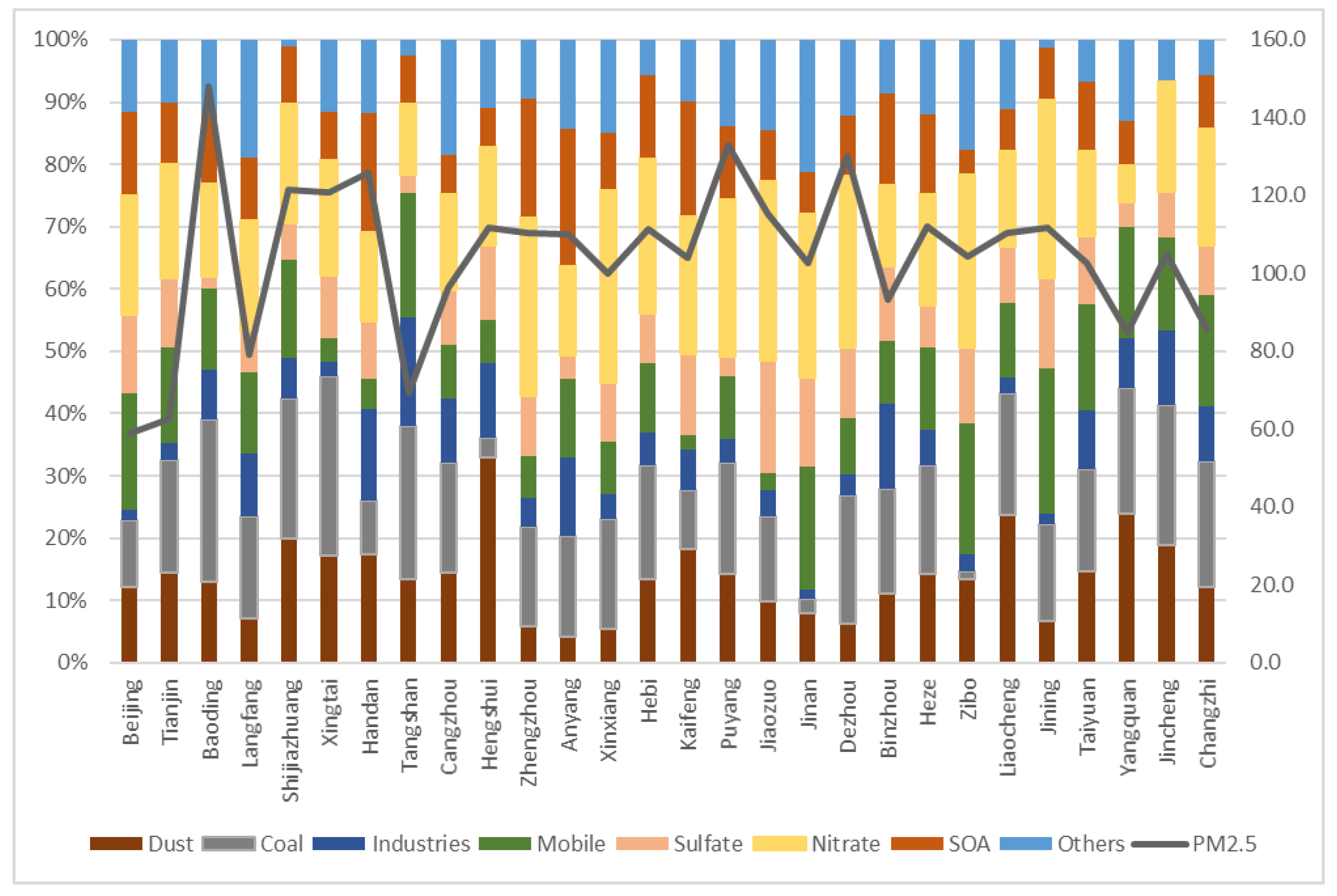
The mobile source was also a significant contributing source sector of PM_2.5 in the region, averagely contributing 12.5% of PM_2.5 concentration. Among the 28 cities, the mobile source contribution also had a significant variation. The largest mobile emissions contributions were found in industrial cities and metropolitan cities. Industrial cities of Jining, Zibo and Tangshan, where diesel truck transportation was important, had the largest contribution of mobile sources of 23.4%, 21.0% and 19.9%, respectively. Metropolitan cities of Beijing, Tianjin, Jinan and Taiyuan also have relatively higher mobile emission contributions of 18.6%, 15.3%, 19.8% and 17.0%, which may be due to the contribution of passenger cars.

On average, the industrial sources only had a marginal contribution of 7.0% to PM_2.5 concentration in the region. Nevertheless, since the industrial contribution in this study is only the primary contribution of the industrial processes without coal combustion, the total contribution of industries would be higher if coal and secondary pollutants were also considered together.

It is important to note that the CMB receptor model cannot resolve the contributions of emission sources to the secondary components of PM_2.5. For the 2+26 Cities Region, considering the high organic fraction and significant secondary organic components (SOA), combined with secondary inorganic ions, the secondary components of PM_2.5 in 28 cities accounted for about or more than half of PM_2.5 concentrations, which most likely involve long-range transport. Source apportionment focusing solely on primary components is insufficient for supporting effective control policymaking.

3.2. Source Apportionment by CTM Model and the Contribution of Lang-Range Transport

CTM models can obtain the complete source contribution results for all PM_2.5 components, including both the primary and secondary components. Using tracking technology, the CTM model can estimate the contribution of specific sources or source groups, specifically for our case, the contribution of different source sectors in various cities. In this work, Comprehensive Air Quality Model with extensions (CAMx) using Particulate Source Apportionment Technology (PSAT). The modeling domain and grids are shown in Fig.2. The CTM models used nesting techniques with 36km grids for whole country and 12km grids for 2+26 Cities Region. The simulation period was from October 2017 to March 2018. The performance of the CAMx model for simulating SO₂, NO₂, CO, O₃, PM_2.5, PM₁₀ concentration and components concentration of PM_2.5, including sulfate, nitrate, BC, OC, and ammonium (NH₄⁺) concentrations was verified against the observed data in the winter of 2018 (MEE, 2020).

The updated emission inventory for 2017 was based on the MEIC2017 for the whole country and updated emissions of the 2+26 Cities Region. Due to differences in industrial development and energy structures, the spatial distribution of air pollutant emissions varies significantly among cities. Beijing and Tianjin are the two largest metropolitan cities in China, where heavy industries were not the major sectors of the economy. Both cities had very low SO₂, PM_2.5 and CO emissions. However, NOx and dust emissions were significant due to the large population of vehicles, traffic and construction. Tangshan, the largest heavy industrial city in the region, has the highest iron and steel production capacity and the highest emissions of PM_2.5, PM₁₀, NOx, and CO, which are significantly higher than those of other cities in the region.

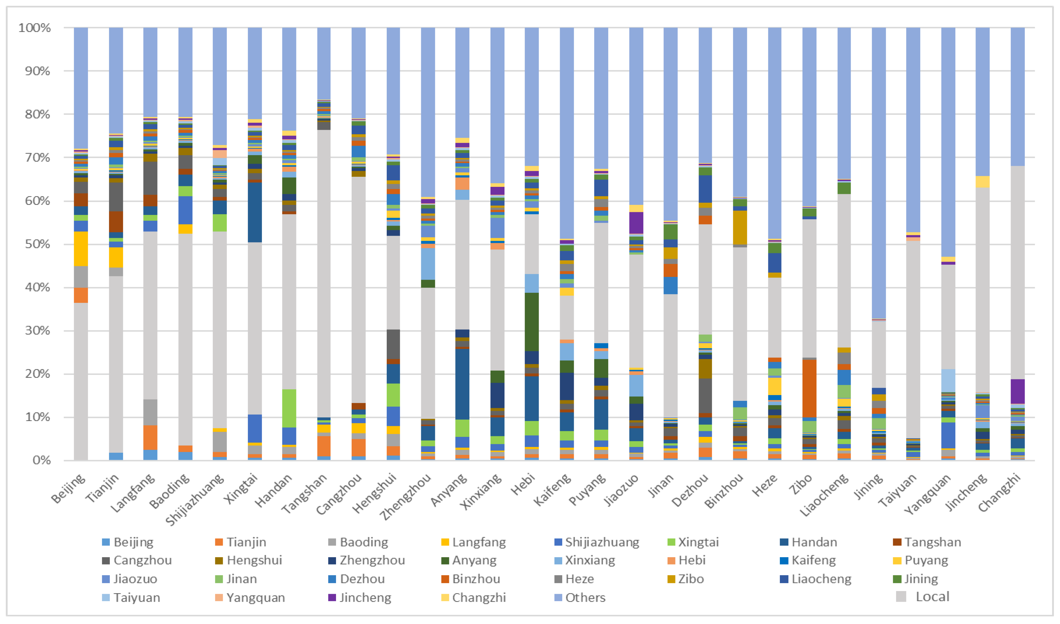
Emissions, especially primary PM_2.5 emissions from local sources, are the important and direct contributors to PM_2.5 concentrations in one city. Nevertheless, emissions from other areas or lang-range transport, especially from neighboring areas, can also play important roles. Long-range transport usually contributes more than local emission sources to the secondary component of PM_2.5. Based on the simulation of the concentrations and source apportionment, CAMx model obtained the local contributions, the regional mutual contributions of cities in the 2+26 Cities Region, and from outside the 2+26 Cities Region cities during the winter of 2017-2018 (Fig.4).

Generally, the PM_2.5 pollution in the 2+26 Cities Region was a regional problem. The cities with small local emissions and small administrative areas have less local contribution and more prominent contributions from outside or long-range transport. Location and meteorology are also important factors. For most cities in the region, the contributions from the sources inside the 2+26 Cities Region were the main contribution. Inside 2+26 Cities Region, the local contributions of the emission sources in the winter of 2017-2018 ranged between 20% and 50%, showing a great variation at the same time. The contributions from outside the 2+26 Cities Region, or background concentrations, were similarly between 20% and 30%. The local contribution to PM_2.5 of Tangshan was 66.5% due to its highest emissions in the region and vast area. The other significant local contributions were found in Cangzhou, Changzhi, Langfang, Jincheng, Shijiazhuang, and Taiyuan, accounting for approximately half of the PM_2.5 concentration, with values of 52.4%, 49.4%, 48.9%, 47.2%, 45.6% and 45.6%, respectively. In the two mega-cities of Beijing and Tianjin, even having vast areas, the local contribution accounted for only 36.5% and 40.9% of PM_2.5 concentrations, respectively, due to the lower emission.

For the secondary component of PM_2.5, the local emissions contributed an average of 30.0% to the sulfate in PM_2.5 in 2+26 cities. Only in Tangshan and Cangzhou of Hebei Province local emissions contributed more than half of the sulfate concentration, accounting for 67.6% and 54.4%. For other cities, especially the cities with both small areas and SO₂ emissions, such as in Henan Province, most sulfate comes from long-range transport. Most of the nitrate and SOA in PM_2.5 in 2+26 cities were contributed by long-range transport. On average, the local emissions contributed only 10.1% of nitrate and 15.1% of SOA in PM_2.5.

On the other hand, for the primary component of PM_2.5, the local contributions were usually significant, with an average of 43.4 % in 2+26 cities. Tangshan, Cangzhou in Hebei province and Jincheng, Changzhi in Shanxi province had the most significant local contributions to the primary component of PM_2.5 of 77.2 %, 65.3%, 62.3% and 63.5%, respectively. Tianjin, and all cities in Hebei province except Hengshui, as well as all cities in Shanxi province except Yangquan, have local emissions that contribute more than 50% of the primary component of PM_2.5. Most cities in Henan and Shandong provinces have less local contribution to primary PM_2.5.

Figure 4. Contribution of emissions from local, the other cities in the 2+26 Cities Region, and the other parts of China.

Figure 4. Contribution of emissions from local, the other cities in the 2+26 Cities Region, and the other parts of China.

3.3. Refined Source Apportionment of Local Emission in 2+26 Cities Region

Based on the multi-model integrated PM_2.5 source apportionment approach described earlier, combining the bulk or first-level source apportionment results by the CMB receptor model and the long-range or trans-boundary transport of the primary and secondary components of PM_2.5 by the CTM model, the local contributions from 15 emission sources sectors to the PM_2.5 concentrations had been resolved. Furthermore, by applying the local emission source inventory, the refined local contribution of specific emission sources or finer emission sectors to local PM_2.5 concentrations has been resolved.

From the refined source apportionment results of PM_2.5 in the 2017-2018 winter in the 2+26 Cities Region (Fig.5), it can be found that the combined coal combustion, including coal-fired boilers, power plants, and household coal burning, was the most significant contributing sector, accounting for an average of 35.1% of local contributions. Among these, the coal-fired boilers sector was the most significant single sector of local contribution, which, on average, accounting for 19.1% of the contribution of local sources. This result showed that the control of coal-fired boilers and residential coal combustion emissions should be priority in the action plan of the cities in the region, especially for the heating season.

The household coal burning, mainly for heating and cooking, was another significant portion of the local contribution, on average accounted for 14.8% of PM_2.5 local contribution (Fig.5). In the winter of 2017-2018, even in Beijing and Tianjin, household coal still accounted for 13.7% and 12.2% of local contribution, respectively, mainly from mountainous suburban areas. Considering the low emission height and nearby locations, the same amount of emission of household coal burning usually causes much higher impact on ground concentration than other emission sources. Therefore, the control of household coal combustion should also be one of the priorities of the control action plan.

On the other hand, even though the coal consumption by power plants was large, due to effective control and high stack emission, the local contributions to PM_2.5 concentrations are small, on average, accounting for only 1.2% of the total local contribution.

Mobile emissions were also significant emission sources in 2+26 cities, especially diesel mobile emission sources). Mobile emissions have a similar contribution as boiler and dust emissions, accounting for 18.0% of local contribution. Diesel mobile source was the second largest single source category contributing to PM_2.5, accounting for 15.6 % of PM_2.5, and 86.7% of the total mobile contribution.

Figure 5. Refined source apportionment of PM_2.5 concentration in 2017-2018 winter (%).

Figure 5. Refined source apportionment of PM_2.5 concentration in 2017-2018 winter (%).

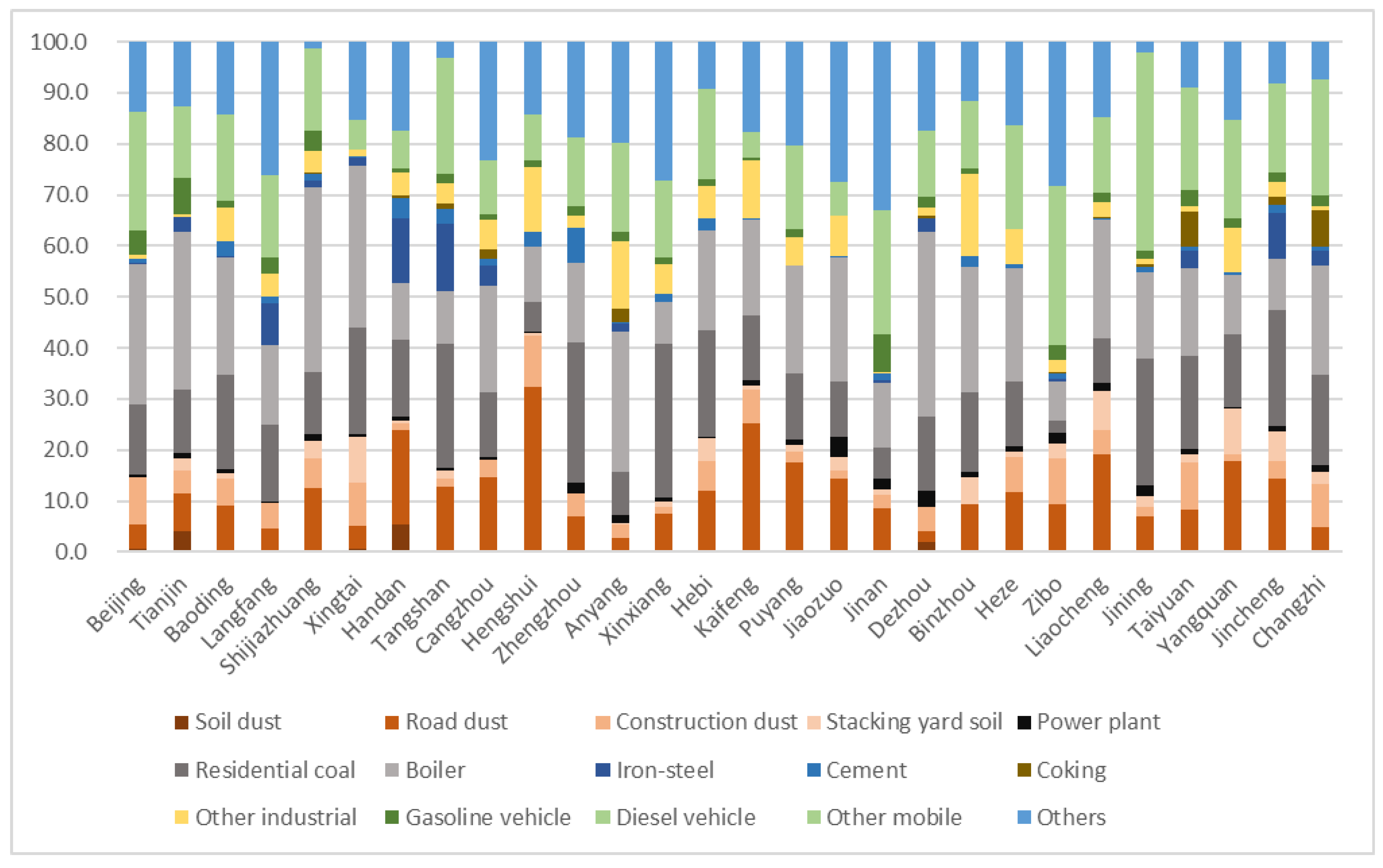
The gasoline mobile emission was not the most significant source for all cities in the winter of 2017-2018. However, in large cities, gasoline cars have made a relatively greater contribution. Jinan, Tianjin, Beijing, Shijiazhuang, and Taiyuan are the five cities with the largest gasoline mobile emission contribution, accounting for local emission contributions of 7.3%, 7.2%,4.7%,4.0%,3.3% respectively. Combined together, mobile emissions and road dust made transportation sector the second-largest contributing sector, accounting for 29.2% of PM_2.5.

The PM_2.5 concentration levels of Beijing and Tianjin, the two megacities in the region, were the lowest among the 28 cities. Beijing does not have coal combustion-related industries, while Tianjin still has some heavy industries in its suburbs, including steel industries. However, in Beijing, boilers were still the biggest PM_2.5 emission source in the winter of 2017, contributing 27.4% of PM_2.5 and about 40% of the local contribution. Mobile emission sources also contributed significantly, contributing 27.3% of PM_2.5, including 22.6% coming from diesel mobile sources, the second largest single contributing emission source, and only 4.7% from approximately 5 million gasoline vehicles. Dust is another important PM_2.5 local source for PM_2.5 in Beijing, accounting for 13.7% of the local contribution of PM_2.5, including 9.3% from construction and 4.8% from road dust.

Similar to Beijing, the emission from boilers was also the largest local emission source of PM_2.5 in Tianjin, accounting for 31.2% of PM_2.5 local contribution. Mobile emissions of Tianjin accounted for 21.2% of the local contribution, which is less than that of Beijing, with 14.0% from diesel mobile emissions and 7.2% from gasoline cars. The total dust contribution was 18.4% in Tianjin, including 4.7% from construction dust, 7.3% from road dust, and 4.1% and 2.4% from soil and stocking yards. The mobile emission contribution in Shijiazhuang, Zhengzhou, Jinan and Taiyuan, the capitals of Hebei, Henan, Shandong, and Shanxi provinces were also relatively high. In Shijiazhuang, Jinan and Taiyuan, mobile emissions accounted for 20.1%, 31.8% and 23.4%, respectively.

4. Conclusions and Discussion

PM_2.5 component measurement data, emission inventory, receptor model, and CTM model provide various kinds and levels of information on source contributions. However, each of these data and source apportionment tools have their own limitations and uncertainties. In this work, we developed a three-step PM_2.5 source apportionment approach integrats PM_2.5 components measurement data and receptor model, emission inventory and CTM model to obtain the refined contributions of emission sources of different emission sectors and locations.

The integrated approach developed in this work has been applied to conduct refined source apportionment in the 2+26 Cities Region during the autumn and winter of 2017-2018, which provided the complete source apportionment results for all components of PM_2.5 with administrative region information, which are important for the development of policy and action plan.

This approach utilizes relatively accurate PM_2.5 component measurement data especially the organic components, dust, and secondary components such as sulfate and nitrate. CMB receptor model can further identify the contributing sources of the primary components of PM_2.5, which can be translated to control policy directly. For the source apportionment for the winter and autumn of 2017-2018, CMB model identified that coal combustion was still the largest single contribution source sector, and dust and mobile source were the other two significant contributing sources. The integrated approach avoids the CTM’s uncertainties such as simulating the organic component and dust components of PM_2.5 due to the difficulties with model mechanisms, emission inventory, and resolution. However, the high secondary components of PM_2.5, source apportionment in 2+26 Cities Regions suggested that focusing solely on primary components is insufficient.

This approach utilizes CTM to estimate the contribution of emission sources of different cities by simulating atmospheric physical and chemical processes and tracking the relative contributions of the source groups by sectors and locations. The CTM model addresses the limitations of receptor models, which cannot resolve secondary components of PM_2.5 and cannot identify the locations or administrative region of contributing emission sources. The source apportionment results of the CTM model provided the important sources contributions information for all components of PM_2.5, including local contributions, mutual contributions among the 28 cities, and contributions from areas outside the 2+26 City Region. The findings of the CTM model regarding spatial contributions suggest that PM_2.5 pollution in the 2+26 Cities Region is primarily a regional issue, largely confined within the 2+26 Cities Region. However, the source apportionment of CTM for organic components cannot be used directly due to the high uncertainties of the SOA mechanism in CTM and the uncertainties of VOCs, primary organic components in the emission inventory. The source apportionment of CTM for dust also cannot be used directly due to the high uncertainties in the emission inventory and resolution of the modeling. However, the relationships between emissions and air concentrations for these species are valid and can be used for integrated source apportionment.

Combining the source apportionment results from both the CMB receptor model and the CTM model, we have obtained the refined source apportionment of local emission sources. Averagely in 2+26 cities, the combined coal combustion sector, including boilers, residences, and power plants, was the largest contributing sector, accounting for 35.1% of total PM_2.5 concentration, while boilers contributed 19.1% and residential coal burning contributed 14.8%, respectively. Mobile emissions contributed another 18.0% of PM_2.5 local contribution, of which 15.6% were from diesel-fueled mobile emissions. Combining road dust and mobile emissions, the emissions from the transportation sector were the second-largest PM_2.5 contributing sector, accounting for a total of 29.2% of PM_2.5 local contribution. This finding suggests the need for more comprehensive control measures in transportation sector. In conclusion, the refined source apportionment results from this work recommended prioritizing policies and action plans targeting coal-fired boilers, residential coal burning, diesel vehicles and other mobile sources, and dust, especially road dust.

Although the integrated source resolution approach in this work attempts to utilize the capability and avoid the weaknesses of the CMB receptor model and the CTM model, some uncertainties remain. As noted above, the necessity of knowing the source categories in advance, combined with the uncertainty in the chemical composition profiles of the emission sources used in the CMB model, inevitably leads to some limitations and errors. At the same time, there were high uncertainties in emission inventory for CTM models, especially for VOCs, dust and organic components of primary PM_2.5 emission. Due to insufficient knowledge about chemical reactions, the discrepancy for secondary components such as sulfate, nitrate, and SOA was still more considerable than that of primary PM_2.5.

It is challenging to directly verify the source apportionment results. However, during the implementation of the Action Plan for Prevention and Control of Air Pollution in the Winter of 2017-2018 (State Council of China, 2013), the countermeasures in the “2+26” cities based on this work and other related research projects (Zhang, Q., 2019) have been implemented. As the result of the Action Plan, in 2018 and following years, the annual average PM_2.5 concentrations in the "2+26" Cities Region decreased drastically. This significant improvement in PM_2.5 concentration level has largely validated the source apportionment results of this study and other related research (Zhang, Q., 2019).

References

- Belis C.A., et al., European guide on air pollution source apportionment with receptor models, JRC technical report to European Commission, revised version 2019.
- Belis, C.A.; Karagulian, F.; Larsen, B.R.; Hopke, P.K. Critical review and meta-analysis of ambient particulate matter source apportionment using receptor models in Europe. Atmospheric Environ. 2013, 69, 94–108. [Google Scholar] [CrossRef]
- Dai, S., Zhu, T., Bai, Z., Application and progress of receptor models in source apportionment of atmospheric particulates. Chinese Journal of Environmental Science, 1995, 4.
- Hopke, P.K. Review of receptor modeling methods for source apportionment. J. Air Waste Manag. Assoc. 2015, 66, 237–259. [Google Scholar] [CrossRef] [PubMed]
- Jacobson, M. Z., Fundamentals of Atmospheric Modeling, Cambridge University Press, May 5, 2005.
- Koo, B.; Wilson, G.M.; Morris, R.E.; Dunker, A.M.; Yarwood, G. Comparison of Source Apportionment and Sensitivity Analysis in a Particulate Matter Air Quality Model. Environ. Sci. Technol. 2009, 43, 6669–6675. [Google Scholar] [CrossRef] [PubMed]
- Kwok, R.; Napelenok, S.; Baker, K. Implementation and evaluation of PM2.5 source contribution analysis in a photochemical model. Atmospheric Environ. 2013, 80, 398–407. [Google Scholar] [CrossRef]
- Liang J., Wang W., Establishment of a regional source apportionment model. Chinese Journal of Environmental Science, 1990, 10(1).
- Ministry of Ecology and Environment of the People's Republic of China. (2012). Ambient Air Quality Standards (GB 3095-2012).
- Ministry of Ecology and Environment (MEE), Project Report of the Source Apportionment of PM2.5 in Beijing-Tianjin-Hebei and Surrounding "2+26" Cities(DQGG0107), National Research Program on Cause and Control of Severe Air Pollution, July 26, 2020.
- Ministry of Ecology and Environment (MEE), People's Republic of China, 2019 Report on the State of Ecology and Environment in China https://english.mee.gov.cn/Resources/Reports/soe/SOEE2019/202012/P020201215587453898053.pdf (accessed March 11, 2025).
- Paatero, P.; Tapper, U. Positive matrix factorization: A non-negative factor model with optimal utilization of error estimates of data values. Environmetrics 1994, 5, 111–126. [Google Scholar] [CrossRef]
- Paatero, P. Least squares formulation of robust non-negative factor analysis. Chemom. Intell. Lab. Syst. 1997, 37, 23–35. [Google Scholar] [CrossRef]
- Seinfeld, J.H.; Pandis, S.N. Atmospheric Chemistry and Physics: From Air Pollution to Climate Change, 2nd ed.; Wile-Interscience: New York, NY, USA, 2006; ISBN 9780471720171. [Google Scholar]
- State Council of P. R. China, Action Plan on the Prevention of Air Pollution, September 2013.
- State Council of China, Three-year Action Plan for Winning the War to Protect Blue Sky, 2018-22, June 27, 2018.
- Tian, Y.-Z.; Shi, G.-L.; Huang-Fu, Y.-Q.; Song, D.-L.; Liu, J.-Y.; Zhou, L.-D.; Feng, Y.-C. Seasonal and regional variations of source contributions for PM10 and PM2.5 in urban environment. Sci. Total. Environ. 2016, 557-558, 697–704. [Google Scholar] [CrossRef] [PubMed]
- Viana, M.; Kuhlbusch, T.A.J.; Querol, X.; Alastuey, A.; Harrison, R.M.; Hopke, P.K.; Winiwarter, W.; Vallius, M.; Szidat, S.; Prévôt, A.S.H.; et al. Source apportionment of particulate matter in Europe: A review of methods and results. J. Aerosol Sci. 2008, 39, 827–849. [Google Scholar] [CrossRef]
- Wagstrom, K.M.; Pandis, S.N.; Yarwood, G.; Wilson, G.M.; Morris, R.E. Development and application of a computationally efficient particulate matter apportionment algorithm in a three-dimensional chemical transport model. Atmospheric Environ. 2008, 42, 5650–5659. [Google Scholar] [CrossRef]
- Wang, Z.S.; Chien, C.; Tonnesen, G.S. Development of a tagged species source apportionment algorithm to characterize three-dimensional transport and transformation of precursors and secondary pollutants. J. Geophys. Res. Atmos. 2009, 114. [Google Scholar] [CrossRef]
- Wang, J.; Xu, J.; He, Y.; Chen, Y.; Meng, F. Long range transport of nitrate in the low atmosphere over Northeast Asia. Atmospheric Environ. 2016, 144, 315–324. [Google Scholar] [CrossRef]
- Wang, D. , Wang, T. , Han, J., Xie, X., Chen, C., Cao, Y., Shu, L. Source apportionment analysis of PM2.5 under severe air pollution in 2+26 cities. Chinese Journal of Environmental Science, 2020, 1, 92–99. [Google Scholar]
- Watson, John G. et al., Protocol for Applying and Validating the CMB Model for PM2.5 and VOC, EPA-451/R-04-001, December 2004a.
- Watson, John G, U.S. EPA, Chemical mass balance receptor model version 8 (CMB) user's manual, EPA-452/R-04-011, December 2004b, Research Triangle Park, NC.
- World Health Organization. (2021). WHO global air quality guidelines: Particulate matter (PM2.5 and PM10), ozone, nitrogen dioxide, sulfur dioxide, and carbon monoxide. World Health Organization.
- Yanjun Zhang, Jing Cai, Shuxiao Wang, Kebin He, Mei Zheng, Review of receptor-based source apportionment research of fine particulate matter and its challenges in China, Science of the Total Environment, Volume 586, May 15, 2017, Pages 917-929.
- Zhao, P. S., Dong, F., He, D., Zhao, X. J., Zhang, X. L., Zhang, W. Z., Yao, Q., and Liu, H. Y.: Characteristics of concentrations and chemical compositions for PM2.5 in the region of Beijing, Tianjin, and Hebei, China, Atmos. Chem. Phys., 2013, 13, 4631–4644. [CrossRef]
- Zhao, X.J.; Zhao, P.S.; Xu, J.; Meng, W.; Pu, W.W.; Dong, F.; He, D.; Shi, Q.F. Analysis of a winter regional haze event and its formation mechanism in the North China Plain. Atmospheric Meas. Tech. 2013, 13, 5685–5696. [Google Scholar] [CrossRef]
- Zhang, Z.; Wang, W.; Cheng, M.; Liu, S.; Xu, J.; He, Y.; Meng, F. The contribution of residential coal combustion to PM 2.5 pollution over China's Beijing-Tianjin-Hebei region in winter. Atmospheric Environ. 2017, 159, 147–161. [Google Scholar] [CrossRef]
- Zhang, Q.; Zheng, Y.; Tong, D.; Shao, M.; Wang, S.; Zhang, Y.; Xu, X.; Wang, J.; He, H.; Liu, W.; et al. Drivers of improved PM2.5 air quality in China from 2013 to 2017. Proc. Natl. Acad. Sci. USA 2019, 116, 24463–24469. [Google Scholar] [CrossRef] [PubMed]
Disclaimer/Publisher’s Note: The statements, opinions and data contained in all publications are solely those of the individual author(s) and contributor(s) and not of MDPI and/or the editor(s). MDPI and/or the editor(s) disclaim responsibility for any injury to people or property resulting from any ideas, methods, instructions or products referred to in the content. |
© 2025 by the authors. Licensee MDPI, Basel, Switzerland. This article is an open access article distributed under the terms and conditions of the Creative Commons Attribution (CC BY) license (http://creativecommons.org/licenses/by/4.0/).
Copyright: This open access article is published under a Creative Commons CC BY 4.0 license, which permit the free download, distribution, and reuse, provided that the author and preprint are cited in any reuse.