
Submitted:
10 August 2025
Posted:
13 August 2025
You are already at the latest version
Abstract
Atmospheric pollution, produced by CO, NO₂, and SO₂, represents a significant risk to health and the environment globally. In regions such as Apurimac, Peru, this problem is aggravated by industrial and vehicular emissions. The study aimed to analyze the spatiotemporal trends of these pollutants between 2020 and 2023 using Sentinel-5P satellite data, to identify critical areas and seasonal variations. Data from the TROPOMI instrument on board Sentinel-5P, processed using Google Earth Engine (GEE), were used to map pollutant concentrations. The analyses were performed with JavaScript algorithms. The study focused on urban, industrial, and mining areas. The results showed elevated CO levels in urban areas, such as Abancay, with peaks reaching up to 150 µg/m³, associated with vehicular traffic and agricultural burning. Critical NO₂ points were located near mining operations with maximum values of 0.375 µg/m³, while SO₂ peaks up to 9.8 µg/m³ coincided with industrial activities. Seasonal increases were observed during the months of pasture burning (August to October). Correlations between pollutants were weak (r = 0.1) for CO, and a coefficient of determination for NO2 (R2 = 0.004), reflecting diverse emission sources. Although concentrations generally remained below World Health Agency (WHO) limits, localized pollution hotspots persist, driven by anthropogenic activities. The study demonstrates the usefulness of GEE for regional air quality monitoring and highlights the need for policies aimed at reducing emissions, especially in mining and urban areas.
Keywords:
air pollution
; sentinel-5P
; GEE
; CO
; NO₂
; SO₂
; Apurímac
1. Introduction
The studies conducted by the World Health Organization in 2016 on atmospheric air pollution reveal that one out of every nine deaths is directly related to atmospheric pollution [1]. At the same time, the Pan American Health Organization [2] indicates that one of the most important factors to be taken into account is the quality of the air where people live, and this problem is directly related to the deaths caused by respiratory diseases due to the inhalation of polluted air. According to [3,4], atmospheric air pollution is one of the environmental problems that occurs primarily in industrialized countries undergoing economic development, generating public health issues at the local, regional, and national levels. On the other hand, the World Health Organization [1] indicates that 90% of the world's population lives in polluted environments, breathing air with high levels of pollution. The consequences of this exposure are generally presented as deaths due to respiratory problems. Many studies, for example, [5], mention that there is a direct relationship between disease and environmental pollution, where NO2, dust (PM2.5, PM10), CO, O3, CH4 gas, and others, create diseases in the health of the population, causing respiratory diseases, cardiovascular diseases and fertility diseases [6,7]. Atmospheric pollution is a global threat that has enormous repercussions on human health and ecosystems. One of the most hazardous pollutants in the atmosphere is nitrogen dioxide (NO2), which is linked to respiratory and cardiovascular diseases, reduced self-cleaning capacity of the respiratory tract, weakening of the immune system in the lungs, and asthma, among other health issues [8].
NO2 is considered the most essential anthropogenic pollutant contributing to the greenhouse effect. It plays a fundamental role in climate change [9], which in turn contributes to the generation of smog, acid precipitation, and the greenhouse effect [3]. CO2 emissions have contributed to a global increase in temperatures worldwide, which has led to the accelerated melting of the polar ice caps and glaciers [10]. Likewise, this contamination is common, caused by various human activities such as deforestation and industrial processes, which exacerbate climate change and contribute to respiratory diseases [5]. Due to the presence of the gas, the population is generally exposed to diseases like asthma and respiratory problems [11]. Even when it enters the atmosphere, it alters air quality. Moreover, [12], which is generally produced by the emission of gases from the operation of internal combustion engines, revealed that 65% is generated by vehicle transportation and the remaining 35% from other sources, such as power plants and the industrial sector. Additionally, one of the primary air quality pollutants of concern to urban and industrial populations worldwide, particularly in countries with high economic development, is NO2, whose maximum permissible limits exceed the established values [13].
CO, for [14], is a toxic gas that can have harmful effects on human health when concentrations are high. On the other hand, we can consider it a silent killer when it accumulates in sectors and places with poor ventilation, where there is little to no airflow. Several studies have shown that environmental pollutants produced in the environment have decreased with the emergence of the COVID-19 disease, due to a decrease in industrial activities, including NO2 and CO, resulting from anthropogenic and industrial sources (15,16). The reduction in NO2 levels in 2020 was observed on a global scale during the COVID-19 pandemic period, associated with population restrictions [17].
SO2 is present in our environment, has detrimental effects on human health, causes respiratory problems when exposed to high concentrations, and contributes to environmental degradation by forming acid rain [18]. For [19,20], the sources of this gas generation include the incomplete combustion of fossil fuels and activities developed to support the local economy, such as transportation, manufacturing, electricity generation, and other sources. Additionally, volcanic eruptions are a source of this gas. Domestic activities, such as burning garbage, charcoal, or wood in stoves, also emit these gases, contributing to air pollution [21].
With the launch into space of the first Copernicus satellite of the European Union, part of the fleet of ESA Sentinel missions, we can monitor the environment, with the launch into space, a great leap was made for the acquisition of open source images for environmental use [22]; with an instrument called TROPOspheric Monitoring that continuously orbits the Earth and performs measurements that allow us to create daily global maps of atmospheric species relevant to the monitoring of air quality and climate [23]. These values of the TROPOMI instrument are used to measure the concentration of pollutants in the troposphere. These data have been evaluated, modeled, and validated by different authors in environmental issues [24]. Likewise, the sensors have been calibrated for downloading parametric data on a global scale with independent measurements for each pollutant, these records are similar to those from NASA sensors [24,25], and the accuracy of the spectrometric measurement was also evaluated at different spatial scales, from local to regional and national levels, with measurements in the ultraviolet, visible, visible-near and shortwave infrared spectra that can provide information on atmospheric data, such as NO2, NO, CH4 gas and O3 gas [26]. Currently, the highest-resolution images available are from TROPOMI, which enables the determination of focal points of pollutant emissions, consolidating its position as one of the most essential instruments for observing atmospheric composition, both now and in the near future [19]. On the other hand, with the help of Sentinel-5 sensor data, it is possible to study environmental problems with daily information on changes in atmospheric pollution in areas that do not have ground stations [27], it has also been possible to examine the relationship between changes in atmospheric pollution and cases of coronavirus mortality, due to the impact of air pollution, affecting public health with respiratory diseases [23]. Many studies indicate that air pollution in urban areas can be reduced if appropriate policies are implemented to control traffic due to urban transportation, vehicle circulation and the various activities that take place in cities with huge industries [15].
The objective of this research work is to check a comparative analysis of the presence of pollutants in the atmosphere of CO, SO2, NO2 concentrations, identifying the sectors with the highest concentration and periods with pollution levels, obtained from Sentinel-5P data products at the level of the Apurimac region, corresponding to the period from 2020 to 2023 within the Google Earth Engine (GEE) environment, using JavaScript algorithms.
2. Materials and Methods
2.1. Study Area
The Apurimac region is located southeast of the central Andes in Peru; its territory is considered the most rugged in the country. It is bordered to the north by the departments of Ayacucho and Cusco, to the northwest, west, and southwest by the department of Ayacucho, to the northeast, east, and southeast by the department of Cusco, and the south by Arequipa (Figure 1). The area covers approximately 2,111,415.20 ha, and the vegetative cover includes a variety of categories, ranging from Andean grasslands, natural and planted forests, to a series of scrubland associations [28]. The area's climate is characterized by a very marked rainy season from December to March, with average temperatures of 16°C, and a dry season the rest of the year, with maximum temperatures of 25°C and minimum temperatures of 8°C [29].
2.2. Materials
The present research work focuses on the Apurimac region, utilizing the following data sources: Sentinel-5P NRTI CO (Near Real-Time Carbon Monoxide), Sentinel-5P NRTI NO2 (Near Real-Time Nitrogen Dioxide), and Sentinel-5P NRTI SO2 (Near Real-Time Sulfur Dioxide), the data used in this study encompass a global scope; in this research, a model of atmospheric gas concentration, including CO, NO2, and SO2, was developed [23]. The methodology employed is based on the use of Geographic Information Systems (GIS) and Remote Sensing, specifically in the analysis and interpretation of images obtained by the Sentinel-5P satellite, using the TROPOMI sensor. The pollutant measurements, which were key to this analysis, are freely available to Google Earth Engine (GEE) users.
2.2.1. CO, NO2, and SO2 Data from the TROPOspheric Monitoring Instrument (TROPOMI)
According to ESA, data on the pollutant CO are present in the atmosphere and are fundamental to understanding tropospheric chemistry. In certain urban areas, its presence is one of the main atmospheric pollutants [30]. The primary sources of CO are fossil fuel combustion, biomass burning, atmospheric oxidation of methane gas, and other hydrocarbons [19]. At the same time, fossil fuel combustion is the primary source of CO in the northern mid-latitudes, and isoprene oxidation and biomass burning play an essential role in the tropics [16]. The TROPOMI instrument retrieves the daily global abundance of CO in both clear and cloudy skies using the 2.3 µm spectral range of the shortwave infrared (SWIR) region. Observations in clear skies are sensitive to CO in the tropospheric boundary layer, while cloudy atmospheres modify the sensitivity of the column as a function of light path variations. It has a resolution of 1113.2 meters, with units in mol/m²—dataset availability: 2018-06-28 - Current, available at the following Link: https://developers.google.com/earth-engine/datasets/catalog/COPERNICUS_S5P_OFFL_L3_CO.
The European Space Agency (ESA), states that the CO pollutant data come from global data obtained in situations of clear and cloudy sky, the noise that is presented makes the data appear negative values, this is observed in the vertical column especially in clean regions or with very low SO2 emissions, for this it is recommended not to filter these negative values except for atypical values, that is to say, vertical columns lower than -0.001 mol/m2 [23].
For NO2 data processing obtained from TROPOMI sensor data, this dataset represents the composite concentration of nitrogen dioxide produced through photochemical cycling during the day, involving ozone and sunlight. The NO2 processing system is based on the algorithm developed for the DOMINO-2 product and the QA4ECV NO2 dataset, which has been reprocessed for OMI and adapted for TROPOMI [31]. This assimilation and absorption modeling system utilizes a three-dimensional TM5-MP global chemical transport model with a 1 ° x 1 ° resolution as an essential element [32]. For CO data, negative values are often observed in the vertical columns due to noise, especially in clean regions with low NO2 emissions. It is also recommended not to filter these values except in the case of outliers, i.e., vertical columns smaller than -0.001 mol/m2 [23]. The data are available at the following link: https://developers.google.com/earth-engine/datasets/catalog/COPERNICUS_S5P_OFFL_L3_NO2
According to the European Space Agency (ESA), SO2 enters the Earth's atmosphere through both natural and anthropogenic processes. It plays a role in local and global-scale chemistry, and its impact ranges from short-term pollution to climate effects. Only about 30% of the SO2 emitted comes from natural sources; most is of anthropogenic origin. SO2 emissions harm human health and air quality [20]. Volcanic SO2 emissions can also be a threat to aviation, along with volcanic ash [33]. Sentinel-5P (S5P) samples the Earth's surface with a revisit time of one day and an unprecedented spatial resolution of 3.5 x 7 km, allowing acceptable detail resolution, including detection of much smaller SO2 plumes [34]. The data are available at the following link: https://developers.google.com/earth-engine/datasets/catalog/COPERNICUS_S5P_OFFL_L3_SO2
2.2.2. Google Earth Engine Platform
The Google Earth Engine (GEE) platform, developed by Google, enables large-scale geospatial processing using a database with millions of data points. One of the primary objectives of this platform is to reduce the time spent on preprocessing and facilitate analyses conducted with geospatial information [34,35]. Additionally, it is a tool that is currently gaining popularity due to its extensive processing capabilities and its speed in analyzing geospatial information [37]. The platform is available at: (https://earthengine.google.com/.
This GEE platform is a free online access that merges "Big Data" technologies, works with Python and JavaScript programming algorithms, among others; it makes available in its database a large number of satellite images, recent and historical data information on a planetary scale, and uses machine learning algorithms for environmental monitoring [36]. The data for this research work are available from 2018 to the present at the following link: https://developers.google.com/earth-engine/datasets/catalog/sentinel-5p
2.2.3. Geographic Information System (GIS)
GIS is currently undergoing an era of exponential development, supported by the increasing availability of new sensors, satellite images, and open georeferenced data, which enable the production of new knowledge about the world and empirical geographic phenomena [38]. The processing of Sentinel-5P satellite images in ArcGIS involves a series of processing steps, first, the data must be downloaded from sources such as the Copernicus Open Access Hub and/or files processed on the GEE platform, then these downloaded files must be decompressed and converted to ArcGIS compatible format, such as GeoTIFF, once imported into ArcGIS, various processing techniques can be applied, such as atmospheric correction, calculation of atmospheric contaminants, time series analysis [39]. Finally, it is essential to note that spatial observation at a global level, facilitated by satellites that capture repetitive images, enables us to conduct environmental studies, such as those related to atmospheric air pollution [40].
3. Methodology
For the analysis and data processing of CO, NO2 and SO2 pollutants, were carried out on the GEE platform, this platform developed by Google allows us to perform large-scale geospatial processing, using databases with millions of these, one of the benefits of this platform is to reduce the time invested in preprocessing and facilitate the analysis performed with geospatial information [36], to catalog and process a wide variety of Earth observation data at no cost and saving time [15,35]. GEE offers two APIs, one in JavaScript, which is accessed via the Internet through a browser and is the most well-known, up-to-date, and user-friendly. It is also the one with the most documentation and help available. On the other hand, there is the Python API, which can be accessed from the Python console and allows, to a certain extent, the complementary use of Python libraries to perform more complex processing or functionalities that the JavaScript API does not support [36]. In the present work, we have processed the data in JavaScript for different periods using Sentinel-5P images; Figure 2 shows the methodology.
4. Results
4.1. Analysis of the Concentration of CO, NO2, and SO2 Pollutants
An exhaustive analysis of CO, NO₂, and SO₂ concentrations was conducted at the monitoring points distributed throughout the study region. The results showed significant fluctuations in the concentrations of these pollutants, which were especially evident during September and October, correlating with the burning of weeds and organic waste. However, traditional practices in some areas, such as agricultural practices, industrial activities, vehicle traffic transporting materials, and the presence of mining companies, among others, have negative consequences for the environment and health.
For the OC period 2020-2023, a significant pattern of pollution concentration levels was observed in densely populated urban areas, especially in the province of Abancay, which does not exceed the threshold recommended by the WHO, whose values range between 100 μg/m³ and 150 μg/m³. Peripheral areas also exhibited very high concentrations of pollutants, as seen in the provinces of Chincheros and Andahuaylas, suggesting that the primary sources of pollution are vehicular traffic in the city center and forest fires caused by human activities [41].
Regarding the pollutant NO₂, the results show a red color (high concentration), with values ranging from 0.20 μg/m3 to 0.35 μg/m3, mostly in urban areas where there is a higher concentration of cars and also in sectors where there are mining operations such as the mining company Las Bambas in Chalhuahuacho, these concentrations are dangerous to health, particularly for people with respiratory problems, and can affect healthy people if exposure is prolonged [12].
The presence of the SO₂ pollutant in the atmosphere is generally classified into different levels according to its impact on human health and the environment. These levels are divided into categories that reflect the concentration of SO₂ in the air, and vary according to international regulations and guidelines, such as those of the World Health Organization (WHO) and national air quality standards. The results show very high levels of the red color spectrum, which are noticeable in several sectors, with values ranging from 7.80 μg/m³ to 10 μg/m³. These values impact air quality and are associated with intensive industrial activities, such as mining or the combustion of fossil fuels.
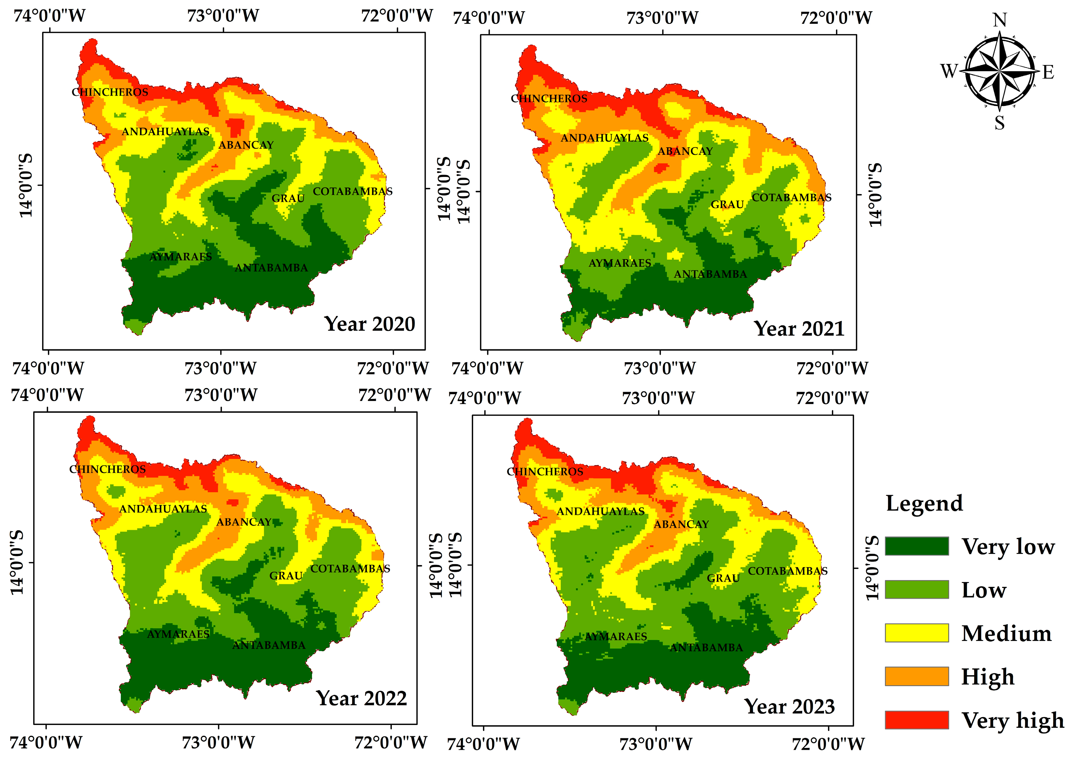
Figure 3.
Data processing of the CO pollutant on the Google Earth Engine platform for the period 2020-2023.
Figure 3.
Data processing of the CO pollutant on the Google Earth Engine platform for the period 2020-2023.

Figure 4.
Data processing of the NO2 pollutant on the Google Earth Engine platform for the period 2020-2023.
Figure 4.
Data processing of the NO2 pollutant on the Google Earth Engine platform for the period 2020-2023.
4.2. Identificación de Los Sectores de Mayor Concentración
The results enabled us to identify key areas where pollutant concentrations were consistently higher. These areas primarily correspond to various sector types, including industrial, urban, and high-traffic zones. The data processing was carried out using Geographic Information System software, which allowed the analysis of carbon monoxide pollution in the Apurimac region, providing detailed visual information illustrating CO concentrations. In 2020 and 2021, the highest CO concentrations were recorded in the provinces of Abancay, Chincheros, and Andahuaylas; medium to high concentrations were observed in the province of Grau, while the lowest were observed in the provinces of Aymaraes. During the periods of 2022 and 2023, exceptionally high concentrations were recorded in the provinces of Abancay, Chincheros, and Andahuaylas.
NO₂ is a pollutant generated by vehicular transport, the burning of fossil fuels, and industrial emissions [42]. The analysis shows that in the 2020, 2021, and 2022 periods, the highest concentrations are found in the province of Cotabambas, followed by the provinces of Grau, Abancay, and Chincheros.
By 2023, NO₂ concentrations are expected to have decreased considerably. Therefore, a reduction in the levels of the pollutant can generally be viewed positively, as it reflects a decrease in pollution sources and an improvement in air quality, since NO₂ is a significant pollutant that contributes to the formation of tropospheric ozone and acid rain [43]. In the province of Cotabambas, the concentration remains very high due to the presence of the Las Bambas Mining Company.
SO₂ is a colorless gas that, in high concentrations, is irritating and harmful to health, originating mainly from the combustion of coal and petroleum derivatives, and can be transformed into sulfuric acid, affecting the respiratory system [44].
According to the data represented in Figure 5, the highest concentrations of SO₂ are expected to be recorded between 2020 and 2023, primarily in the provinces of Cotabambas, Anta-bamba, Aymaraes, and Grau, with Aymaraes exhibiting the highest concentration values. During the years 2021 and 2022, lower levels were observed throughout the Apurimac region compared to 2020 and 2023, as shown in the raster images in the figure, which indicate intensive industrial activities such as mining or burning fossil fuels.
4.3. Determination of the Variability of Concentration with Time
The temporal variability of pollutant concentrations from 2020 to 2023 was evaluated to understand better the daily, weekly, and seasonal fluctuations of the pollutants. It was found that CO concentration showed a high concentration the month of October 2020 with peak traffic concentrations, taking values up to 150 μg/m3, while NO₂ and SO₂ concentrations presented more complex patterns, with notable peaks in September and October 2022 with concentrations reaching 0.355 μg/m3 of NO2 specific conditions, such as days of high industrial activity, and agricultural activities. Figure 6 shows the con-centration for the period 2020 and 2023, a significant variability was observed in carbon monoxide (CO) con-centrations in different regions, during the study period, the highest concentrations were recorded in densely populated urban areas, especially in August, September and October that fluctuate in average values of 120 μg/m3, In the 2020 period, October reached the highest peak at a value of 150 μg/m3 and also in November 2023, due to increased weed and shrub burning, summarizing, concentrations decreased in the summer months, favored by greater atmospheric dispersion corresponding to the months from May to August with values ranging from 40 μg/m3 to 90 μg/m3.
The analysis revealed a general trend of decreasing average CO concentrations, which was attributed in part to the implementation of stricter environmental policies and a reduction in vehicle traffic during the COVID-19 pandemic in 2021 and 2022. However, specific events, such as forest fires in tropical and subtropical regions, caused temporary spikes in CO concentrations during drought months.
Figure 6.
Time series of the atmospheric pollutant CO in the GEE period 2020-2023.
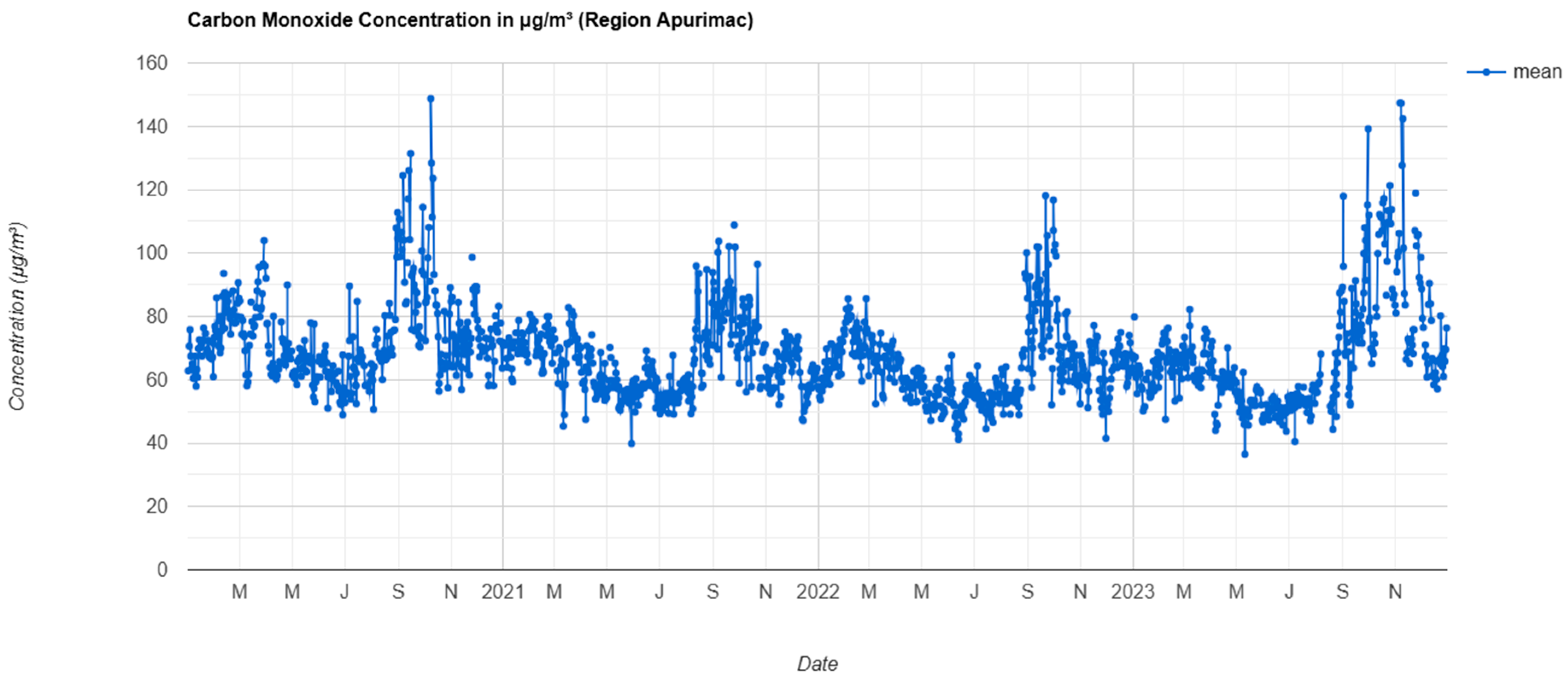
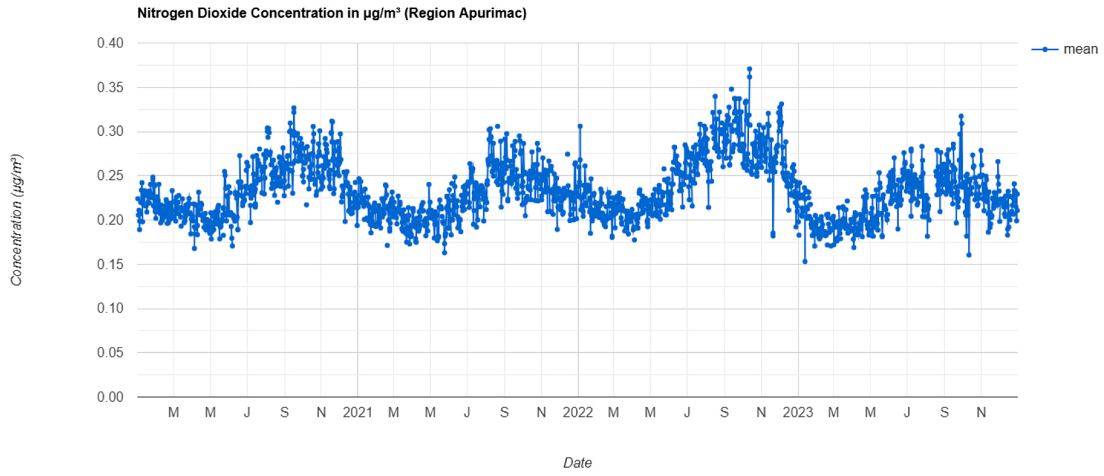
Figure 7, corresponding to the time series of the NO2 pollutant for 2022, shows significant variation throughout the year. It is observed that in September and October, concentrations reach a maximum value of up to 0.375 μg/m³, while during April to September, a gradual increase is identified. Subsequently, concentrations decrease from October to March, reaching a minimum value of 0.150 μg/m3.
A combination of anthropogenic and natural factors can explain these fluctuations. During October and periods of highest concentration, emissions associated with human activities, such as vehicular traffic, industry, and biomass burning, intensify. In addition, meteorological conditions, such as atmospheric stability and low temperatures, can favor the accumulation of pollutants by limiting vertical dispersion.
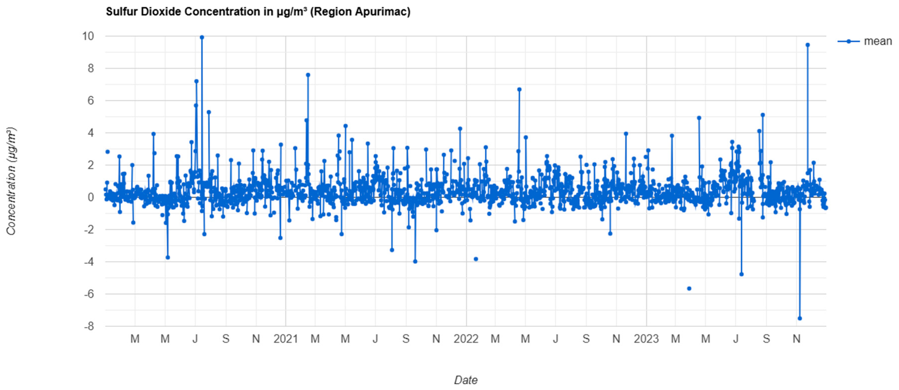
In the time series simulation in the (GEE) platform for the period 2020 to 2023, the analysis of variability in sulfur dioxide (SO2) concentrations revealed clear patterns in both natural and anthropogenic emissions. Significant peaks of SO2 were observed in July 2020, reaching a value of 10 μg/m³. The month of February 2021 reached a value of 7.8 μg/m3. In 2023, the months outside of November reached a value of 9.8 μg/m3. Likewise, the lowest peaks occurred in the remaining months, reaching a minimum value of 0.0 μg/m³ during the study period.
Figure 8.
Time Series of SO2 Air Pollutant in the GEE Period 2020-2023.
4.4. Correlation Analysis of Pollutants Concerning Time
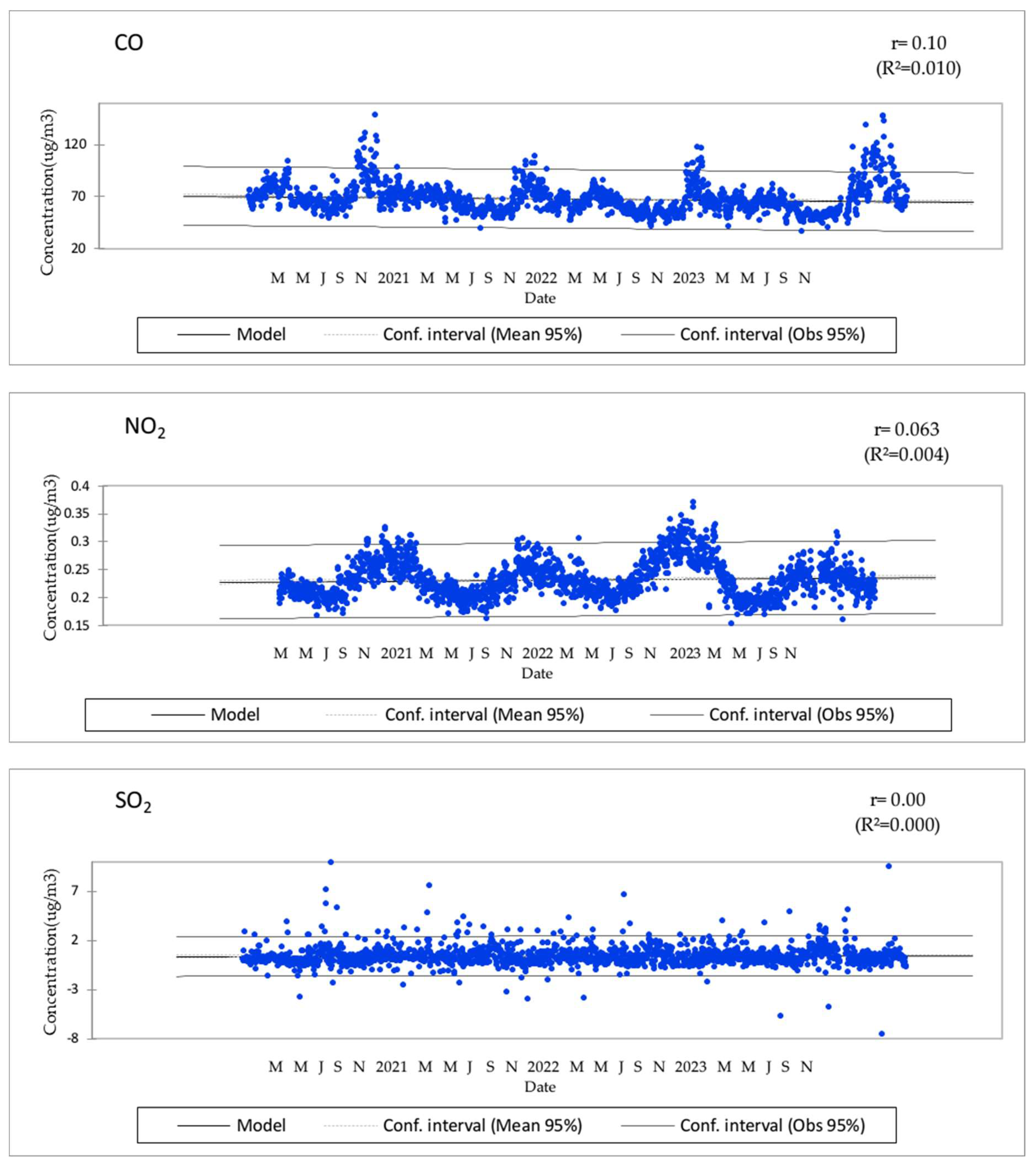
The temporal variability of pollutant concentrations from 2020 to 2023 was evaluated to understand daily better, weekly, and seasonal fluctuations. It was found that CO concentration showed a very low correlation r=0.10, [45] at peak traffic hours, especially in urban areas with a coefficient of determination of R2= 0.010, while NO₂ and SO₂ concentrations presented more complex patterns with coefficients of determination values of R2= 0.004 for NO2 and R2= 0.000, very low peaks. Comparison with other countries with industrial activities, such as China, the United States, and other industrialized countries like Italy [46], reports values of R² = 0.85 in northern Italy and R² = 0.71 in southern Italy. Likewise, the concentrations in South Korea found a similar coefficient of determination R2= 0.48 for hourly data and R2 = 0.77 for annual data, for the NO2 surface concentrations obtained from the S-5P TVCD NO2 product over South Korea [47], these values are shown to be very high compared to the values obtained in the Apurimac region, where air pollution oscillates with very low values that are not very representative.
Figure 9.
Coefficient of Determination (R²) of the pollutants CO, NO₂, and SO₂.
5. Discussion
The present study analyzed the concentrations of atmospheric pollutants carbon monoxide (CO), nitrogen dioxide (NO₂), and sulfur dioxide (SO₂) in the Apurímac region from 2020 to 2023, using satellite images from TROPOMI on board the Sentinel-5P satellite and processed through the Google Earth Engine platform. The results show that the concentrations of these gases show significant spatio-temporal variability, influenced by human activity, topography, and seasonal climatic factors.
The average concentrations of CO, NO₂, and SO₂ remained at levels generally below the permissible thresholds established by the WHO. However, critical accumulation zones were identified in dense urban areas and the vicinity of mining complexes. This finding is consistent with previous studies that relate mining activity and urban transportation as primary sources of pollutant gas emissions [15]. The statistical correlation between gas concentrations was weak, indicating the absence of a direct linear relationship between the variables analyzed, which may be attributed to the multicausal nature of emissions and differences in atmospheric transport and dispersion processes. Seasonally, concentration peaks were observed in August and September, coinciding with the traditional agricultural practice of pasture burning, which increases temporary CO and NO₂ emissions. This phenomenon aligns with patterns reported in regional and international studies, where controlled or accidental biomass burning generates punctual increases in atmospheric contaminants [48]. Likewise, satellite data showed a reduction in emissions during 2020, following mobility restrictions due to the COVID-19 pandemic, and a rebound in 2021, resulting from the progressive reestablishment of economic activities and the lack of adequate public policies to control vehicular and industrial emissions [15].
At the international level, [48], reported in their multiannual analysis on emissions in the United States, a strong correlation between NO₂ and CO₂ concentrations (r = 0.75), suggesting a common source of origin, mainly related to the burning of fossil fuels. In addition, a more pronounced reduction of CO₂ was documented in regions with high forest cover during summer, attributed to the biological sink effect. Although these results are not directly extrapolable to Apurímac, they allow us to establish helpful analogies on the relationship between vegetation cover, industrial activity, and air quality.
On the other hand, [49] found that urban NO₂ emissions are significantly higher in industrialized regions, such as Europe and China, compared to countries in South Asia and Africa, where cleaner energy sources or less intensive activities predominate. In addition, an increase in emissions was observed during the winter, which is consistent with the seasonal behavior detected in our study, where NO₂ and SO₂ emissions tend to increase in the colder months, possibly due to the use of more polluting heating and fuels. Finally, the results obtained in GEE confirm its effectiveness as an environmental monitoring tool, as Sentinel-5P images showed high sensitivity in detecting seasonal and spatial variations of the analyzed gases, agreeing with the findings reported by [50]. This approach allows the development of early warning systems and evidence-based decision-making to mitigate the effects of air pollution in vulnerable regions such as Apurimac.
6. Conclusions
The study analyzed the temporal trends and spatial distribution characteristics of six primary atmospheric air pollutants—NO2, CO, and SO2—in the Apurimac region from 2020 to 2023, using Sentinel-5P satellite data. It examined atmospheric pollution and evaluated the levels of pollutants throughout the province that comprises the region. The main conclusions of the study are:
(1) NO2 and CO concentrations show a continuous increasing trend, while SO2 remained relatively stable or showed slight decreases. All three pollutants exhibited pronounced seasonal variations in September and October. CO reached its maximum values in the spring months, with high levels in urban areas such as the provinces of Abancay, Chincheros, and Andahuaylas, due to vehicular traffic and forest fires, and decreased in the autumn season. NO2 reached its maximum value in the spring, concentrating primarily in provinces with the highest population and in sectors where mining companies operate, and has since shown a downward trend in the fall. SO2 concentrations were higher in sectors where there is little to no tree vegetation, particularly in places located at higher altitudes.
(2) The temporal variability of pollutant concentrations over time, such as CO, reaches a coefficient of determination of R²= 0.010, while NO₂ and SO₂ concentrations presented very low patterns with values of R²= 0.004 for NO2 and R²= 0.000 or almost nothing. Although CO continued to show a positive correlation in some areas of higher population density, suggesting that its formation is influenced by the presence of automobile fleets, industrial, and mining areas.
The study concludes that urban NO2 emissions exhibit clear seasonal patterns, with an increase during the early spring months, coinciding with high air temperatures resulting from the burning of pastures to initiate sowing. The research problem was solved by identifying geographic and seasonal variations in CO, NO2, and SO2 emissions. Additionally, the study's implications include improving the estimation of emissions and contributing to pollution control policies informed by satellite data.
These results indicate that pollution in the Apurimac is caused by a combination of human activities, including both industrial and agricultural sources, and that several factors must be considered to understand better how pollutants behave in this region. For a more comprehensive analysis, it would be beneficial to combine satellite data with local measurements and to consider meteorological and sociological variables.
Finally, it is recommended that studies continue to be conducted to help design more effective strategies for monitoring and reducing air pollution, thereby protecting the health of the population and the environment in Apurimac.
Author Contributions
Conceptualization, W.H., R.Z., N.M. and E.V.; Investigation, D.S., H.Y., E.V., W.H., F.A. and E.L.; Methodology, R.Z., N.M. and E.L.; Formal analysis, W.H., D.S., H.Y. and E.L.; Data curation, D.S., R.Z., N.M. and H.Y.; Validation, R.Z., F.A., D.S. and E.L.; Project administration, E.C., N.M. and H.Y.; Visualization, R.Z., N.M., H.Y., E.L., W.H. and D.S.; Resources, E.V., H.Y., D.S. and E.L.; Software, W.H., E.V. and E.L.; Supervision, R.Z., D.S. and E.L.; Funding acquisition, W.H., R.Z., D.S., N.M., F.A., H.Y., E.V. and E.L.; Writing—original draft, R.Z., D.S., N.M. and E.V.; Writing—review & editing, W.H., R.Z., D.S., N.M., H.Y., E.V., and E.L. All authors have read and agreed to the published version of the manuscript.
Funding
Not Funding.
Data Availability Statement
The data will be made available upon request.
Acknowledgments
The authors would like to thank the European Space Agency (ESA) and the Copernicus program for providing the Sentinel-5P satellite data used in this study. We are also grateful to the anonymous reviewers for their constructive comments and suggestions, which significantly improved the quality of this manuscript. The authors appreciate the Universidad Nacional Micaela Bastidas de Apurímac (UNAMBA) for their support. Finally, the authors have expressed their gratitude to Walquer Huacani.
Conflicts of Interest
The authors declare that they have no conflicts of interest.
References
- OMS. Organizacion Mundial de la Salud [Internet]. 2016. Available from: https://www.paho.org/annual-report-2016/Espanol.html.
- OPS. Panamericana de Salud Pública [Internet]. 2020. Available from: https://www.paho.org/journal/es/100-anos-revista-panamericana-salud-publica.
- Olmo NRS, Saldiva PH do N, Braga ALF, Lin CA, Santos U de P, Pereirai LAA. A review of low-level air pollution and adverse effects on human health: Implications for epidemiological studies and public policy. Clinics. 2011;66[4]:681–90. [CrossRef]
- Lavaine, E. An Econometric Analysis of Atmospheric Pollution, Environmental Disparities and Mortality Rates. Springer [Internet]. 2014;60(60):215–42. Available from: https://link.springer.com/article/10.1007/s10640-014-9765-0#citeas. [CrossRef]
- Perez L, Declercq C, Inĩguez C, Aguilera I, Badaloni C, Ballester F, et al. Chronic burden of near-roadway traffic pollution in 10 European cities (APHEKOM network). Eur Respir J. 2013;42[3]:594–605. [CrossRef]
- Cesaroni G, Stafoggia M, Galassi C, Hilding A, Hoffmann B, Houthuijs D, et al. Long term exposure to ambient air pollution and incidence of acute coronary events : prospective cohort study and meta-analysis in 11 European cohorts from. 2014;7412(January):1–16. [CrossRef]
- Slama R, Bottagisi S, Solansky I, Lepeule J, Giorgis-Allemand L, Sram R. Short-term impact of atmospheric pollution on fecundability. Epidemiology. 2013;24(6):871–9. [CrossRef]
- Geneva: World Health Organization. WHO global air quality guidelines. Part matter (PM25 PM10), ozone, nitrogen dioxide, sulfur dioxide carbon monoxide. 2021;1–360.
- Mak HWL, Ng DCY. Spatial and socio-classification of traffic pollutant emissions and associated mortality rates in high-density hong kong via improved data analytic approaches. Int J Environ Res Public Health. 2021;18[12]. [CrossRef]
- Calsin WH, Penã NPM, Ochoa ENL, Aguirre Huillcas F, Silva FE. Analisis multitemporal del glaciar del ampay por medio de la plataforma de google earth engine, periodo 2000-2019. CICIC 2021 - Undecima Conf Iberoam Complejidad, Inform y Cibern Memorias. 2021;(Cicic):71–6.
- Li Y, Wang Y, Rui X, Li Y, Li Y, Wang H, et al. Sources of atmospheric pollution: a bibliometric analysis. Springer [Internet]. 2017;(112):1025–1045. Available from: https://link.springer.com/article/10.1007/s11192-017-2421-z#citeas.
- Baldasano, JM. COVID-19 lockdown effects on air quality by NO2 in the cities of Barcelona and Madrid (Spain). Sci Total Environ. 2020;741[2]. [CrossRef]
- Vîrghileanu M, Săvulescu I, Mihai BA, Nistor C, Dobre R. Nitrogen dioxide (No2) pollution monitoring with sentinel-5p satellite imagery over europe during the coronavirus pandemic outbreak. Remote Sens. 2020;12[21]:1–29. [CrossRef]
- Borsdorff T, Aan De Brugh J, Hu H, Hasekamp O, Sussmann R, Rettinger M, et al. Mapping carbon monoxide pollution from space down to city scales with daily global coverage. Atmos Meas Tech. 2018;11[10]:5507–18. [CrossRef]
- Shami S, Ranjgar B, Bian J, Khoshlahjeh Azar M, Moghimi A, Amani M, et al. Trends of CO and NO2 Pollutants in Iran during COVID-19 Pandemic Using Timeseries Sentinel-5 Images in Google Earth Engine. Pollutants. 2022;2[2]:156–71. [CrossRef]
- Vellalassery A, Pillai D, Marshall J, Gerbig C, Buchwitz M, Schneising O, et al. Using TROPOspheric Monitoring Instrument (TROPOMI) measurements and Weather Research and Forecasting (WRF) CO modelling to understand the contribution of meteorology and emissions to an extreme air pollution event in India. Atmos Chem Phys. 2021;21(7):5393–414. [CrossRef]
- Bauwens M, Compernolle S, Stavrakou T, Müller JF, van Gent J, Eskes H, et al. Impact of Coronavirus Outbreak on NO2 Pollution Assessed Using TROPOMI and OMI Observations. Geophys Res Lett. 2020;47[11]:1–9. [CrossRef]
- Jion MMMF, Jannat JN, Mia MY, Ali MA, Islam MS, Ibrahim SM, et al. A critical review and prospect of NO2 and SO2 pollution over Asia: Hotspots, trends, and sources. Vol. 876, Science of the Total Environment. Elsevier; 2023. p. 162851. [CrossRef]
- Opio R, Mugume I, Nakatumba-Nabende J. Understanding the trend of NO2, SO2 and CO over East Africa from 2005 to 2020. Atmosphere (Basel). 2021;12[10]. [CrossRef]
- Wang C, Wang T, Wang P, Wang W. Assessment of the Performance of TROPOMI NO2 and SO2 Data Products in the North China Plain: Comparison, Correction and Application. Remote Sens. 2022;14[1].
- Langley Dewitt H, Gasore J, Rupakheti M, Potter KE, Prinn RG, De Dieu Ndikubwimana J, et al. Seasonal and diurnal variability in O3, black carbon, and CO measured at the Rwanda Climate Observatory. Atmos Chem Phys. 2019;19[3]:2063–78. [CrossRef]
- Paul I, Veihelmann B, Langen J, Lamarre D, Stark H, Courrèges-Lacoste GB. Requirements for the GMES Atmosphere Service and ESA’s implementation concept: Sentinels-4/-5 and -5p. ScienceDirect. 2012;120:58–9.
- Sari NM, Sidiq Kuncoro MN. Monitoring of Co, No2 and So2 Levels During the Covid-19 Pandemic in Iran Using Remote Sensing Imagery. Geogr Environ Sustain. 2021;14[4]:183–91. [CrossRef]
- Zeng J, Vollmer BE, Ostrenga DM, Gerasimov I V, Goddard N, Flight S. Air Quality Satellite Monitoring by TROPOMI on Sentinel-5P. 2019;[2]:10500849. Available from: http://www.essoar.org/doi/10.1002/essoar.10500849.1.
- Beirle S, Borger C, Dörner S, Li A, Hu Z, Liu F, et al. Pinpointing nitrogen oxide emissions from space. Sci Adv. 2019;5[11]:1–7. [CrossRef]
- Theys N, Hedelt P, De Smedt I, Lerot C, Yu H, Vlietinck J, et al. Global monitoring of volcanic SO 2 degassing with unprecedented resolution from TROPOMI onboard Sentinel-5 Precursor. Sci Rep. 2019;9[1]:1–10. [CrossRef]
- Grzybowski PT, Markowicz KM, Musiał JP. Estimations of the Ground-Level NO2 Concentrations Based on the Sentinel-5P NO2 Tropospheric Column Number Density Product. Remote Sens. 2023;15[2]. [CrossRef]
- HUACANI W, MEZA NP, SANCHEZ DD, HUANCA F. Land Use Mapping Using Machine Learning, Apurímac-Peru Region. 2022;176–87.
- Villacorta S, Rodriguez C, Peña F, Jaimes F, Luza C. Caracterización geodinámica y dendrocronología como base para la evaluación de procesos geohidrológicos en la cuenca del río Mariño, Abancay (Perú). Ser Correl Geol. 2016;32(1–2):25–42.
- Borsdorff T, Reynoso AG, Maldonado G, Mar-Morales B, Stremme W, Grutter M, et al. Monitoring CO emissions of the metropolis Mexico City using TROPOMI CO observations. Atmos Chem Phys. 2020;20[24]:15761–74. [CrossRef]
- Liu S, Valks P, Pinardi G, Xu J, Chan KL, Argyrouli A, et al. An improved TROPOMI tropospheric NO2 research product over Europe. Atmos Meas Tech. 2021;14[11]:7297–327. [CrossRef]
- Ialongo I, Virta H, Eskes H, Hovila J, Douros J. Comparison of TROPOMI/Sentinel-5 Precursor NO2 observations with ground-based measurements in Helsinki. Atmos Meas Tech. 2020;13[1]:205–18. [CrossRef]
- Krotkov N, Realmuto V, Li C, Seftor C, Li J, Brentzel K, et al. Day–night monitoring of volcanic so2 and ash clouds for aviation avoidance at northern polar latitudes. Remote Sens. 2021;13[19]:1–18. [CrossRef]
- Corradini S, Guerrieri L, Brenot H, Clarisse L, Merucci L, Pardini F, et al. Tropospheric volcanic so2 mass and flux retrievals from satellite. The etna december 2018 eruption. Remote Sens. 2021;13[11]. [CrossRef]
- Gorelick N, Hancher M, Dixon M, Ilyushchenko S, Thau D, Moore R. Google Earth Engine: Planetary-scale geospatial analysis for everyone. Remote Sens Environ [Internet]. 2017;202:18–27. [CrossRef]
- Perilla SGA, Solorzano VJV. Cómo usar Google Earth Engine y no fallar en el intento [Internet]. México UNA de, editor. Centro de Investigaciones en Geografía Ambiental Universidad Nacional Autónoma de México Instituto de Investigación de Recursos Biológicos Alexander von Humboldt; 2022. 177 p. Available from: http://hdl.handle.net/20.500.11761/36058.
- Kumar L, Mutanga O. Google Earth Engine applications since inception: Usage, trends, and potential. Remote Sens. 2018;10[10]:1–15. [CrossRef]
- McMaster R, Manson S. Geographic Information Systems and Science. Manual of Geospatial Science and Technology, Second Edition. 2010. 513–523 p.
- Trivedi R, Bergi J. Application of GIS for Detection of Ambient Air Pollution of Industrial Area of Gujarat. 2022;[2].
- Chuvieco E. Fundamentos de Teledetección Espacial [Internet]. 84-321-3127-X I, editor. España; 1996. Available from: https://dialnet.unirioja.es/servlet/libro?codigo=630495.
- Casallas A, Cabrera A, Guevara-Luna MA, Tompkins A, González Y, Aranda J, et al. Air pollution analysis in Northwestern South America: A new Lagrangian framework. Sci Total Environ. 2024;906(September 2023). [CrossRef]
- Jamali S, Klingmyr D, Tagesson T. Global-scale patterns and trends in tropospheric no2 concentrations, 2005–2018. Remote Sens. 2020;12[21]:1–18. [CrossRef]
- Bassani C, Vichi F, Esposito G, Falasca S, Di Bernardino A, Battistelli F, et al. Characterization of Nitrogen Dioxide Variability Using Ground-Based and Satellite Remote Sensing and In Situ Measurements in the Tiber Valley (Lazio, Italy). Remote Sens. 2023;15[15]. [CrossRef]
- Chihana S, Mbale J, Chaamwe N. Unveiling the Nexus: Sulphur Dioxide Exposure, Proximity to Mining, and Respiratory Illnesses in Kankoyo: A Mixed-Methods Investigation. Int J Environ Res Public Health. 2024;21(7). [CrossRef]
- Hernández Sampieri R, Fernández Collado C, Baptista Lucio P. Metodología de la Investigación. 6.a ed. McGraw-Hill, editor. México; 2014.
- Cersosimo A, Serio C, Masiello G. TROPOMI NO2 tropospheric column data: Regridding to 1 km grid-resolution and assessment of their consistency with in situ surface observations. Remote Sens. 2020;12[14]. [CrossRef]
- Jeong U, Hong H. Assessment of tropospheric concentrations of no2 from the tropomi/sentinel-5 precursor for the estimation of long-term exposure to surface no2 over south korea. Remote Sens. 2021;13[10]. [CrossRef]
- Xu A, Xiang C. Assessment of the Emission Characteristics of Major States in the United States using Satellite Observations of CO2, CO, and NO2. Atmosphere (Basel). 2024;15[1]. [CrossRef]
- Fioletov V, Mclinden CA, Griffin D, Zhao X, Eskes H. Global seasonal urban, industrial, and background NO 2 estimated from TROPOMI satellite observations. 2024;[2]:1–38. [CrossRef]
- Kazemi Garajeh M, Laneve G, Rezaei H, Sadeghnejad M, Mohamadzadeh N, Salmani B. Monitoring Trends of CO, NO2, SO2, and O3 Pollutants Using Time-Series Sentinel-5 Images Based on Google Earth Engine. Pollutants. 2023;3[2]:255–79. [CrossRef]
Figure 1.
Location of the Apurimac region.
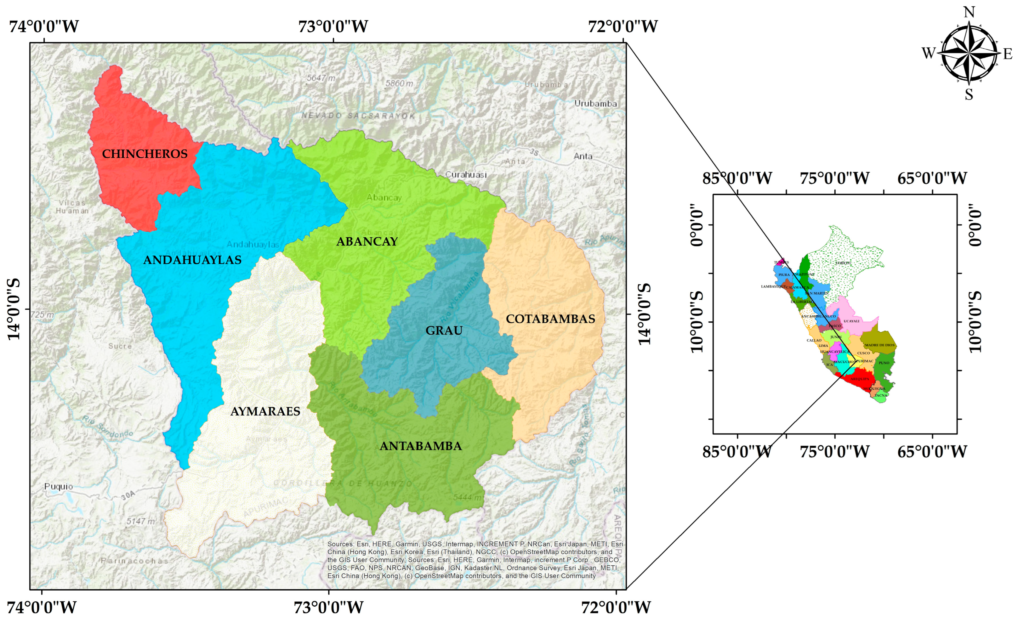
Figure 2.
The process of producing air pollutants maps in the GEE.
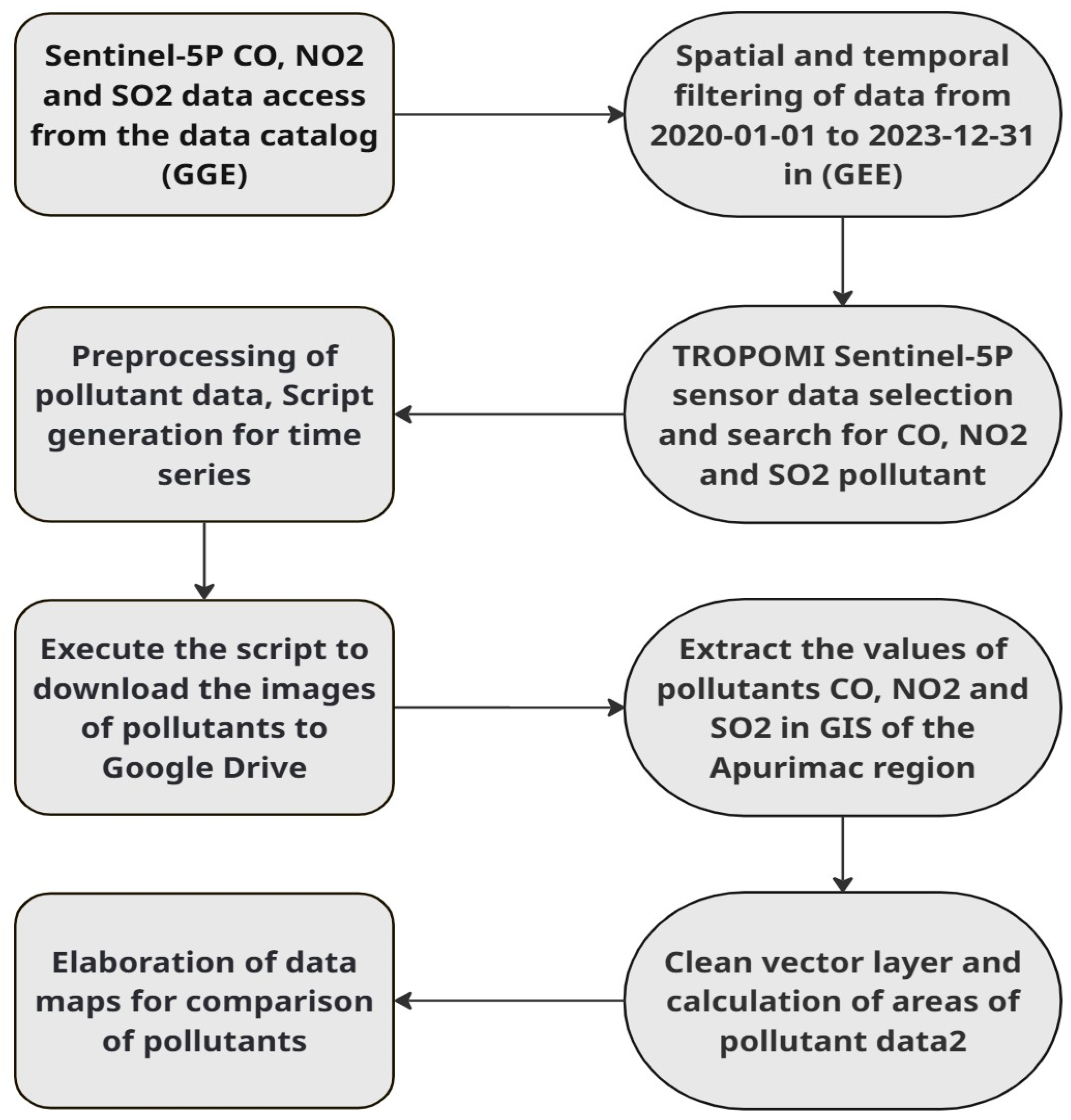
Figure 5.
Data processing of the SO2 pollutant on the Google Earth Engine platform for the period 2020-2023.
Figure 5.
Data processing of the SO2 pollutant on the Google Earth Engine platform for the period 2020-2023.
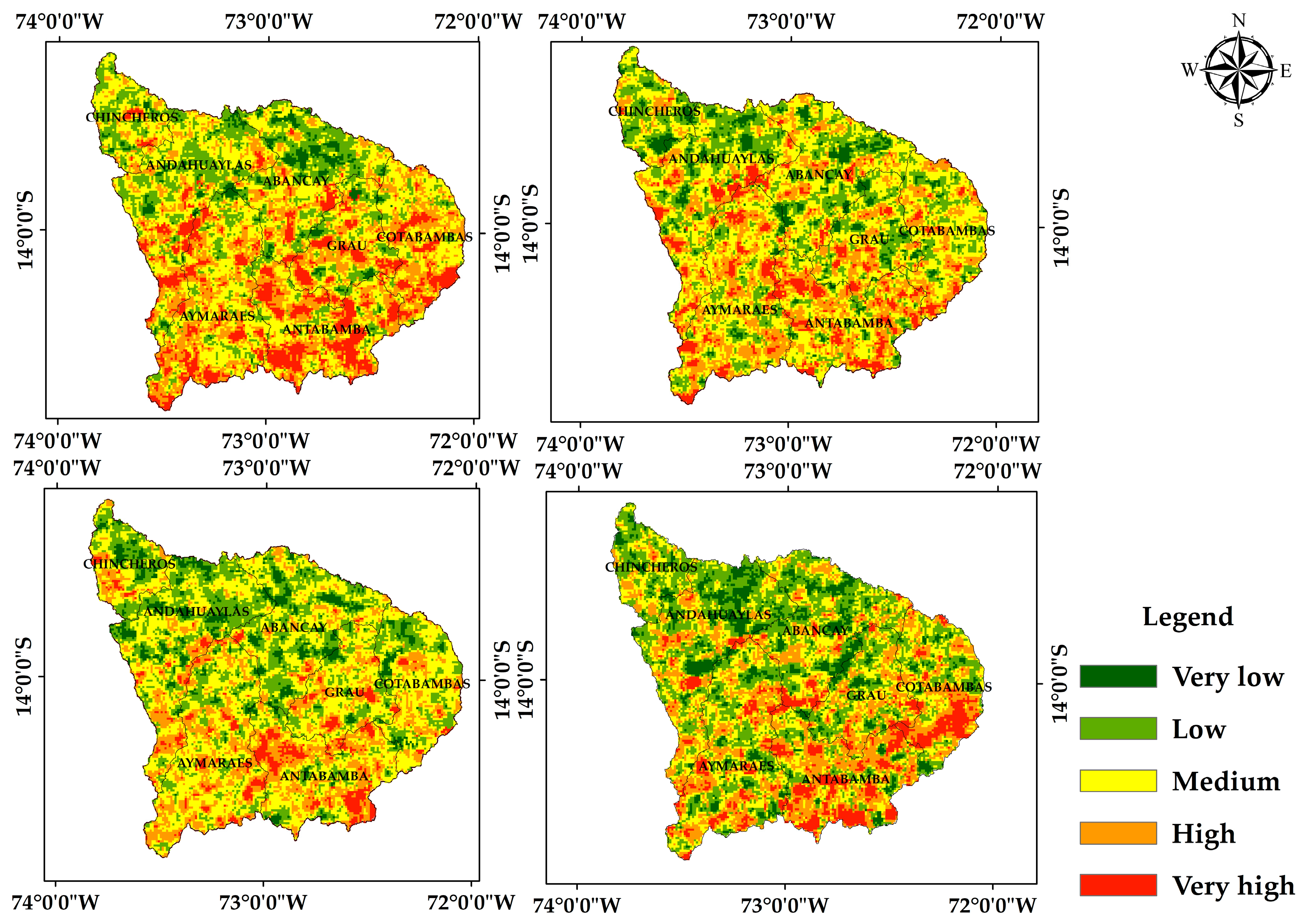
Figure 7.
Time series of the air pollutant NO2 in the GEE period 2020-2023.
Disclaimer/Publisher’s Note: The statements, opinions and data contained in all publications are solely those of the individual author(s) and contributor(s) and not of MDPI and/or the editor(s). MDPI and/or the editor(s) disclaim responsibility for any injury to people or property resulting from any ideas, methods, instructions or products referred to in the content. |
© 2025 by the authors. Licensee MDPI, Basel, Switzerland. This article is an open access article distributed under the terms and conditions of the Creative Commons Attribution (CC BY) license (https://creativecommons.org/licenses/by/4.0/).
Copyright: This open access article is published under a Creative Commons CC BY 4.0 license, which permit the free download, distribution, and reuse, provided that the author and preprint are cited in any reuse.


