
Submitted:
07 July 2025
Posted:
08 July 2025
You are already at the latest version
Abstract
This study investigated the spatiotemporal dynamics of four major air pollutants—carbon monoxide (CO), nitrogen dioxide (NO₂), sulfur dioxide (SO₂), and ozone (O₃)—across Dhaka City from 2020 to 2024 using Sentinel-5P TROPOMI satellite data. A 60-month time-series analysis was conducted, integrating spatial mapping, seasonal composites, and Mann-Kendall trend testing. Results indicated clear seasonal variations: CO and NO₂ concentrations peaked during winter, with maximum monthly averages of 0.05287 mol/m² and 0.00035 mol/m², respectively, while SO₂ reached a high of 0.00043 mol/m² in pre-monsoon months. In contrast, O₃ peaked in May (0.13023 mol/m²), following an inverse seasonal trend driven by photochemical activity. Spatial analysis revealed persistent pollution hotspots in central-western zones like Tejgaon and Mirpur for CO and NO₂, while SO₂ was concentrated in southern industrial zones such as Keraniganj and Jatrabari. The Mann-Kendall test identified moderate to strong increasing trends for CO (τ = 0.8, p = 0.086 in June and September) and SO₂ (τ = 0.8, p = 0.086 in April and May), although most trends lacked statistical significance due to the limited temporal window. This study demonstrates the viability of combining satellite remote sensing and cloud-based processing for urban air quality monitoring and provides actionable insights for targeted seasonal interventions and evidence-based policymaking in Dhaka’s evolving urban context.
Keywords:
urban air pollution
; Sentinel-5P
; Google Earth Engine (GEE)
; Dhaka city
; CO
; NO₂
; SO₂
; O₃
; spatiotemporal analysis
; Mann-Kendall trend test
1. Introduction
Air pollution has emerged as one of the most pressing environmental and public health challenges of the 21st century, particularly in densely populated and rapidly urbanizing cities in the Global South. The World Health Organization (WHO) estimates that air pollution contributes to approximately 7 million premature deaths globally each year, with urban populations facing disproportionately high exposure to harmful pollutants [1]. Among the most critical urban air pollutants are carbon monoxide (CO), nitrogen dioxide (NO₂), sulfur dioxide (SO₂), and ground-level ozone (O₃), each of which poses unique risks to human health, ecosystems, and the climate[2,3]. These pollutants are primarily emitted from anthropogenic sources, including vehicular exhaust, industrial activities, fossil fuel combustion, and biomass burning [4]. As cities continue to grow, understanding the spatiotemporal dynamics of these pollutants becomes essential for effective environmental governance and sustainable urban planning.
In South Asia, Bangladesh—particularly its capital, Dhaka—has been identified as one of the cities with the worst air quality in the world [5]. Dhaka’s complex urban structure, high population density, unregulated industrial clusters, and chronic traffic congestion contribute to persistent and often severe air pollution episodes. Despite growing public concern, monitoring air quality in Dhaka has been hampered by limitations in ground-based sensor networks, including sparse spatial coverage, inconsistent data availability, and maintenance issues [6,7]. These limitations necessitate the integration of satellite remote sensing technologies for continuous, consistent, and large-scale monitoring of atmospheric pollutants.
In recent years, the launch of the European Space Agency’s Sentinel-5P satellite—equipped with the TROPOspheric Monitoring Instrument (TROPOMI)—has revolutionized atmospheric monitoring by providing high-resolution, near-real-time data on key trace gases at a global scale [8]. Sentinel-5P offers daily coverage and spatial granularity sufficient to detect intra-urban pollution variations, making it especially valuable for cities like Dhaka. Coupled with cloud-based geospatial platforms such as Google Earth Engine (GEE), which enables large-scale environmental data processing, researchers now have powerful tools to assess both the spatial and temporal patterns of air pollutants with unprecedented detail and continuity [9].
Several recent studies have demonstrated the utility of Sentinel-5P data in urban air quality monitoring across different contexts. For instance, Bauwens et al. [10] used Sentinel-5P to assess reductions in NO₂ during COVID-19 lockdowns worldwide. Similarly, Matandirotya et al. [11] analyzed SO₂ and CO over African megacities, while Biswas et al. [12] explored pollution trends in Indian cities. However, there remains a significant research gap in applying these advanced tools for long-term, high-resolution air pollution trend analysis in Bangladeshi cities. Most existing studies in Dhaka focus on short-term assessments, use sparse in-situ data, or analyze only one or two pollutants [10,13,14]There is a lack of integrated, multi-pollutant studies that capture both spatial and temporal variations in air quality over multiple years.
To address this gap, the present study aims to monitor and analyze the spatiotemporal dynamics of four major urban air pollutants—CO, NO₂, SO₂, and O₃—over Dhaka city using Sentinel-5P satellite data processed through Google Earth Engine. By constructing a continuous 60-month (January 2020–December 2024) time-series of monthly pollutant concentrations, this research provides one of the most comprehensive assessments of long-term air pollution trends in Dhaka to date.
This research contributes to the growing body of work on satellite-based air quality monitoring by providing a detailed, multi-pollutant assessment of Dhaka’s atmospheric environment. The study reveals emerging seasonal patterns, potential pollution hotspots, and trend directions for each pollutant, offering valuable information for policymakers, urban planners, and public health officials. By linking satellite-based insights with urban management goals, the findings underscore the potential for remote sensing and cloud computing to support data-driven environmental governance in rapidly growing cities of the Global South.
The remainder of this paper is structured as follows. Section 2 outlines the materials and methods, detailing the study area, data sources, satellite processing in Google Earth Engine (GEE), spatial analysis in ArcGIS Pro, Python-based automation, and the application of the Mann-Kendall trend test. Section 3 presents the results, including temporal and seasonal pollutant variations, interannual trends, spatial distributions, and statistical trend assessments. Section 4 provides an in-depth discussion of the observed patterns, highlighting their meteorological, anthropogenic, and spatial drivers. This section also explores the policy implications of the findings, emphasizing targeted interventions for urban air quality management. Finally, Section 5 concludes the study by summarizing the key insights and offering recommendations for integrating satellite-based air quality assessments into evidence-driven urban planning.
2. Materials and Methods
We employed a multi-platform geospatial and remote sensing approach to examine the spatiotemporal variations of key urban air pollutants over Dhaka city from January 2020 to December 2024. Our methodological framework integrated satellite-based atmospheric data, cloud-based remote sensing processing, desktop GIS analysis, and Python-based automation to extract, analyze, and visualize monthly and seasonal patterns of carbon monoxide (CO), nitrogen dioxide (NO₂), sulfur dioxide (SO₂), and ozone (O₃). The entire workflow consisted of several interlinked stages, including study area delineation, data acquisition and preprocessing, time-series pollutant derivation in Google Earth Engine (GEE), and spatial mapping and analysis in ArcGIS Pro.
2.1. Study Area
This study focused on Dhaka city, the capital and largest urban center of Bangladesh, which is recognized as one of the most densely populated and polluted cities globally [15]. We delineated the study boundary using an administrative shapefile of Dhaka, obtained from the Bangladesh Bureau of Statistics (BBS), representing the Dhaka City Corporation area. The shapefile was projected to WGS 84 UTM 46 N and used as a consistent clipping mask throughout our processing. The spatial extent of the study area ranged approximately from 23.67°N to 23.90°N latitude and from 90.33°E to 90.51°E longitude and has an area of 305.82 km2. The area is characterized by dense urban infrastructure, high traffic emissions, and rapid industrialization—factors contributing significantly to air quality deterioration. Figure 1 and Figure 2 show the location and upazila (Upazila is the level 3 administrative boundary in Bangladesh) boundary of the study area respectively.
Dhaka has a tropical wet and dry climate, characterized by hot, humid conditions and a distinct monsoon season. Temperatures generally range from 18°C (64°F) in January to 29°C (84°F) in August, with an annual average of 25°C (77°F). The rainy season, influenced by monsoons, typically occurs from April to September, with June seeing the heaviest rainfall. The driest period is from November to March [16]
The air and water in Dhaka are becoming more and more polluted due to the city’s constantly growing population. To meet the demands of the growing population, multistory buildings and real estate developments are taking up wetland and green space, endangering the city’s biodiversity and urban ecosystem [14].
2.2. Data Sources and Acquisition
We utilized Level 3 (L3) tropospheric column concentration products from the Sentinel-5 Precursor (Sentinel-5P) satellite, which is equipped with the Tropospheric Monitoring Instrument (TROPOMI). This instrument provides daily global measurements of several atmospheric pollutants at a spatial resolution of up to 7 × 3.5 km² (after August 2019), making it suitable for urban-scale air quality analysis [8]. The pollutant-specific datasets used were:
- CO: COPERNICUS/S5P/OFFL/L3_CO;
- NO₂: COPERNICUS/S5P/OFFL/L3_NO2;
- SO₂: COPERNICUS/S5P/OFFL/L3_SO2;
- O₃: COPERNICUS/S5P/OFFL/L3_O3.
We accessed and processed these datasets directly from the Google Earth Engine (GEE) platform, which offers high-performance cloud-based geospatial computation and analysis tools. In total, 60 months of data were acquired and analyzed for each pollutant, covering January 2020 to December 2024. Additionally, we used auxiliary data including Dhaka’s administrative boundary and OpenStreetMap (OSM) layers for contextual mapping.
2.3. Data Processing in Google Earth Engine
All pollutant-specific atmospheric datasets were processed using JavaScript in the GEE code editor. We filtered the Sentinel-5P datasets temporally and spatially to extract pollutant concentrations over Dhaka on a monthly basis. Each ImageCollection was filtered using the ee.Filter.date() function to isolate data for each month. Spatially, we applied the .clip() function using the Dhaka shapefile to confine the dataset to our study boundary.
To ensure the quality and reliability of satellite-derived measurements, we applied a quality assurance (QA) filtering step for each dataset. We applied a quality assurance threshold of QA > 0.75 to filter out low-quality retrievals, following established practice in TROPOMI NO₂ and SO₂ studies [17,18,19,20]. This threshold effectively removes pixels affected by clouds, snow/ice, and retrieval noise, ensuring high-confidence data for spatial and temporal analyses.
Monthly mean composites were generated using the ImageCollection.mean() function in GEE. These monthly average images were then exported in GeoTIFF format to Google Drive using the Export.image.toDrive() function, with a resolution of 0.01 degrees (~1 km) and a bounding box matching the extent of Dhaka. We developed a modular and reusable GEE script that looped through each month and pollutant type to automate the composite generation and export process. This significantly reduced processing time and ensured consistency across the 60-month dataset.
2.4. Spatial Analysis and Visualization in ArcGIS Pro
We performed the spatial analysis and visualization of pollutant data using ArcGIS Pro 3.x, which served as the principal desktop GIS platform for integrating, processing, and interpreting the Sentinel-5P-derived outputs. After exporting the monthly raster layers for CO, NO₂, SO₂, and O₃ from Google Earth Engine (GEE) as GeoTIFF files, we imported these into ArcGIS Pro and organized them systematically in raster catalogs corresponding to each pollutant. This structured organization facilitated batch processing, visualization, and temporal analysis of the 60 monthly rasters (January 2020–December 2024) for each pollutant.
We also generated annual and seasonal average maps by performing raster algebra operations using the “Raster Calculator” tool. Monthly rasters were grouped by year or season (i.e., winter, pre-monsoon, monsoon, and post-monsoon) and averaged to create composite layers representing intra-annual variability. These composites were crucial for identifying persistent pollution zones and for comparing spatial distribution changes over the years.
To support time-series visualization, we used the “Time Slider” tool in ArcGIS Pro. We assigned timestamps to each raster layer and created spatiotemporal animations to illustrate the dynamic monthly changes in pollutant distribution. This technique enabled an intuitive understanding of pollutant behavior and seasonality across years.
2.5. Python-Based Automation Within ArcGIS Pro
To streamline repetitive tasks such as map production, data export, and temporal plotting, we implemented Python scripting through ArcGIS Pro’s built-in Jupyter Notebook environment. Using the ArcPy module, we automated tasks including:
- Batch map generation with consistent layouts (legend, north arrow, scale bar, title);
- Exporting raster statistics to CSV files for each month and pollutant;
- Plotting pollutant trends over time using matplotlib and pandas;
- Performing raster calculations (e.g., difference maps between years).
This automation significantly improved the efficiency of our workflow and reduced the likelihood of human error in processing large volumes of spatial data.
2.6. Temporal Trend and Seasonal Analysis
To capture temporal variability, we categorized each month into four major seasons typical of South Asian monsoonal climates: Winter (December–February), Pre-monsoon (March–May), Monsoon (June–September), and Post-monsoon (October–November) [21]. For each season, we computed seasonal mean composites by averaging the monthly raster layers within each seasonal group. Annual means were also computed by averaging all 12 monthly composites for each year from 2020 to 2024. The resulting seasonal and yearly rasters were used to analyze intra-annual fluctuations and interannual trends in pollutant levels.
We further calculated percent changes in annual pollutant concentrations using raster algebra functions. Trend analysis graphs were generated using time-series data exported from zonal statistics, helping to visualize upward or downward trends across the study period.
2.7. Monthly Trend Detection Using Mann-Kendall Test
To statistically assess monotonic trends in pollutant concentrations over time, we conducted the non-parametric Mann-Kendall (MK) trend test on the monthly average values of CO, NO₂, SO₂, and O₃ for the 60-month period (January 2020 to December 2024). The Mann-Kendall test is widely used in environmental time-series analysis due to its robustness to missing data, non-normal distributions, and its ability to detect both increasing and decreasing trends without assuming linearity [22,23,24].
For each pollutant, we extracted monthly mean concentration values for the entire Dhaka city using the “Zonal Statistics as Table” tool in ArcGIS Pro. The output tables were exported as CSV files and processed in Python using the pymannkendall package, which implements the original Mann-Kendall test along with the modified versions for seasonality and serial correlation correction.
The test was applied to the time-series for each pollutant, yielding the Kendall’s tau coefficient, p-value, and trend classification (increasing, decreasing, or no trend). A significance level of α = 0.05 was adopted to determine whether the observed trend was statistically significant. This step allowed us to quantitatively evaluate long-term changes in atmospheric pollutant concentrations and validate observed patterns in the spatiotemporal maps.
The Mann-Kendall results were then integrated with the spatial analysis by visualizing the statistically significant trends alongside mapped changes in pollutant concentrations. This combination of visual and statistical trend assessment enabled a more comprehensive interpretation of urban air quality dynamics in Dhaka.
3. Results
This section presents the findings of the spatiotemporal analysis of four key atmospheric pollutants—carbon monoxide (CO), nitrogen dioxide (NO₂), sulfur dioxide (SO₂), and ozone (O₃)—over Dhaka City from January 2020 to December 2024. The results are organized to highlight both temporal and spatial patterns, including monthly and seasonal variations, interannual trends, and statistically assessed changes using the Mann-Kendall trend test. Furthermore, spatial distribution maps and zone-wise comparisons reveal intra-urban pollution hotspots and potential source-attribution patterns. All findings are derived from Sentinel-5P TROPOMI satellite data processed through Google Earth Engine and analyzed in ArcGIS Pro, ensuring consistency and high-resolution coverage across the 60-month study period. The results are reported in mol/m², and pollutant-specific characteristics are examined to uncover both meteorological and anthropogenic influences on air quality dynamics in Dhaka.
3.1. Temporal Variation of Pollutants (2020–2024)
3.1.1. Carbon Monoxide (CO)
The monthly mean CO concentrations over Dhaka displayed a distinct seasonal pattern, peaking during winter and declining through the summer monsoon (Figure 3). January recorded the highest mean (0.05136 mol/m²), with the maximum concentration reaching 0.05287 mol/m² and the mode at 0.05195 mol/m². In contrast, July presented the lowest mean (0.03364 mol/m²), minimum (0.03279 mol/m²), and mode (0.03345 mol/m²). The standard deviation was highest in January (0.00064), indicating greater variability during colder months, while June–September had the lowest standard deviations (approx. 0.00029–0.00033), reflecting more stable pollutant levels (Table A1).
3.1.2. Nitrogen Dioxide (NO₂)
Monthly average NO₂ concentration (2020-2024) in Dhaka city has been presented in Figure 4. NO₂ also exhibited pronounced winter peaks and summer lows. January and December had the highest means (0.00030 and 0.00029 mol/m², respectively), with corresponding maxima (0.00035 and 0.00035 mol/m²). July marked the lowest average concentration (0.000081 mol/m²) and also showed the smallest standard deviation (0.000010), suggesting uniformly low NO₂ levels during monsoon months. The highest variability occurred in March and November (standard deviations: ~0.000030), suggesting increased fluctuation in emissions during seasonal transitions (Table A1).
3.1.3. Ozone (O₃)
O₃ concentrations exhibited an inverse seasonal pattern. According to Figure 5, the mean was highest in May (0.13004 mol/m²) and lowest in December (0.11476 mol/m²). Maximum values peaked in May (0.13023 mol/m²) and minimums were lowest in January (0.11639 mol/m²). The lowest standard deviation was recorded in June (0.000045), showing remarkably consistent levels during early monsoon. Mode values across all months closely aligned with mean values, indicating normally distributed data and low skewness in O₃ concentrations (Table A1).
3.1.4. Sulfur Dioxide (SO₂)
SO₂ showed high variability across seasons and zones. As shown in Figure 6, February and March had the highest mean concentrations (0.00030 and 0.00030 mol/m²), with maxima reaching up to 0.00043 mol/m². The lowest means were observed in July (0.000029 mol/m²), with minimums as low as 0.0000 mol/m², reflecting near-absence of SO₂ in some zones during monsoon. High standard deviations, especially in January (0.000064) and November (0.000058), suggest sporadic and spatially concentrated emissions, while July and August exhibited the lowest variability (Table A1).
3.2. Interannual Trends of Pollutants
Figure 7 presents the year-wise monthly trends of four key urban pollutants—CO, NO₂, O₃, and SO₂—over Dhaka from 2020 to 2024. Each pollutant exhibits distinct seasonal and interannual variations in line with meteorological cycles, urban activity levels, and anthropogenic emission sources.
CO concentrations consistently peak during the winter months (December–February) across all years. The highest monthly average values were recorded in January and March, while the lowest concentrations occurred during the monsoon (June–August), especially in July 2022 (~0.033 mol/m²). The CO trends also demonstrate relatively consistent seasonal cycles year-to-year, though 2020 and 2024 showed higher winter values compared to other years. The multi-year mean concentration ranged from 0.0336 to 0.0514 mol/m², with standard deviation peaking in January (0.00064 mol/m²), indicating greater temporal variability during colder months.
NO₂ exhibited sharp seasonal contrast, with peak concentrations during January–March, and the lowest in July–August. Across the years, 2022 recorded the highest NO₂ levels in winter months, while 2024 showed the lowest in March and April. The mean concentrations ranged between 0.00008 and 0.00030 mol/m², with maximum values reaching 0.00035 mol/m² (January). Standard deviation values were lowest during monsoon, indicating reduced temporal variation due to uniform wet deposition.
Unlike the primary pollutants, O₃ displayed an opposite seasonal pattern, with maximum values observed in April–May and a consistent decline from June to December. The annual peak concentration exceeded 0.130 mol/m² during May of 2024. All years follow the same seasonal curvature, driven by photochemical processes, though interannual differences are subtle. Monthly standard deviation remained low (as little as 0.000045 mol/m² in June), indicating stable O₃ formation conditions.
SO₂ showed the highest interannual and intra-month variability. Concentrations peaked during January–March, particularly in 2020 and 2022, with values surpassing 0.0008 mol/m² in January 2022. In contrast, monsoon values (June–August) dropped to near zero in all years. The sharp fluctuations and high standard deviations (up to 0.000064 mol/m²) point to episodic, localized emissions likely from brick kilns and small-scale industries.
Interannual variations highlight the year 2022 as having the highest winter concentrations across all pollutants except O₃, which peaked in 2024. By contrast, 2023 saw relatively suppressed pollution levels, possibly influenced by improved emission control or climatic anomalies such as stronger monsoonal winds.
3.3. Monthly Mann-Kendall Trend Test Over 2020 to 2024
The Mann-Kendall trend test was applied to monthly maximum concentrations of four key atmospheric pollutants (CO, NO₂, SO₂, and O₃) over Dhaka city from 2020 to 2024. The analysis aimed to assess temporal patterns and detect statistically significant trends over this five-year period.
According to Figure 8, CO exhibited predominantly increasing trends across most months, notably in June and September with a Kendall’s Tau of 0.8 and a p-value of 0.086, indicating a near-significant upward trend. Moderate increasing trends were also observed in April, May, and August (Tau = 0.4; p = 0.462). In contrast, February, March, November, and December showed decreasing trends, though none were statistically significant (p > 0.05).
According to Figure 9, NO₂ displayed a mix of trends, with decreasing tendencies in February, March, September, October, November, and December. The steepest downward trend occurred in September (Tau = -0.6; p = 0.220), though it was not statistically significant. Other months like January, April, and August showed no discernible trend (Tau = 0).
As presented in Figure 10, For SO₂, strong increasing trends were identified in April and May (Tau = 0.8; p = 0.086), indicating potential temporal growth in SO₂ levels during pre-monsoon months. Mild upward trends were noted in March and July, while slight to moderate decreases were observed in August, September, November, and December. These changes, however, were not statistically significant at the 0.05 level.
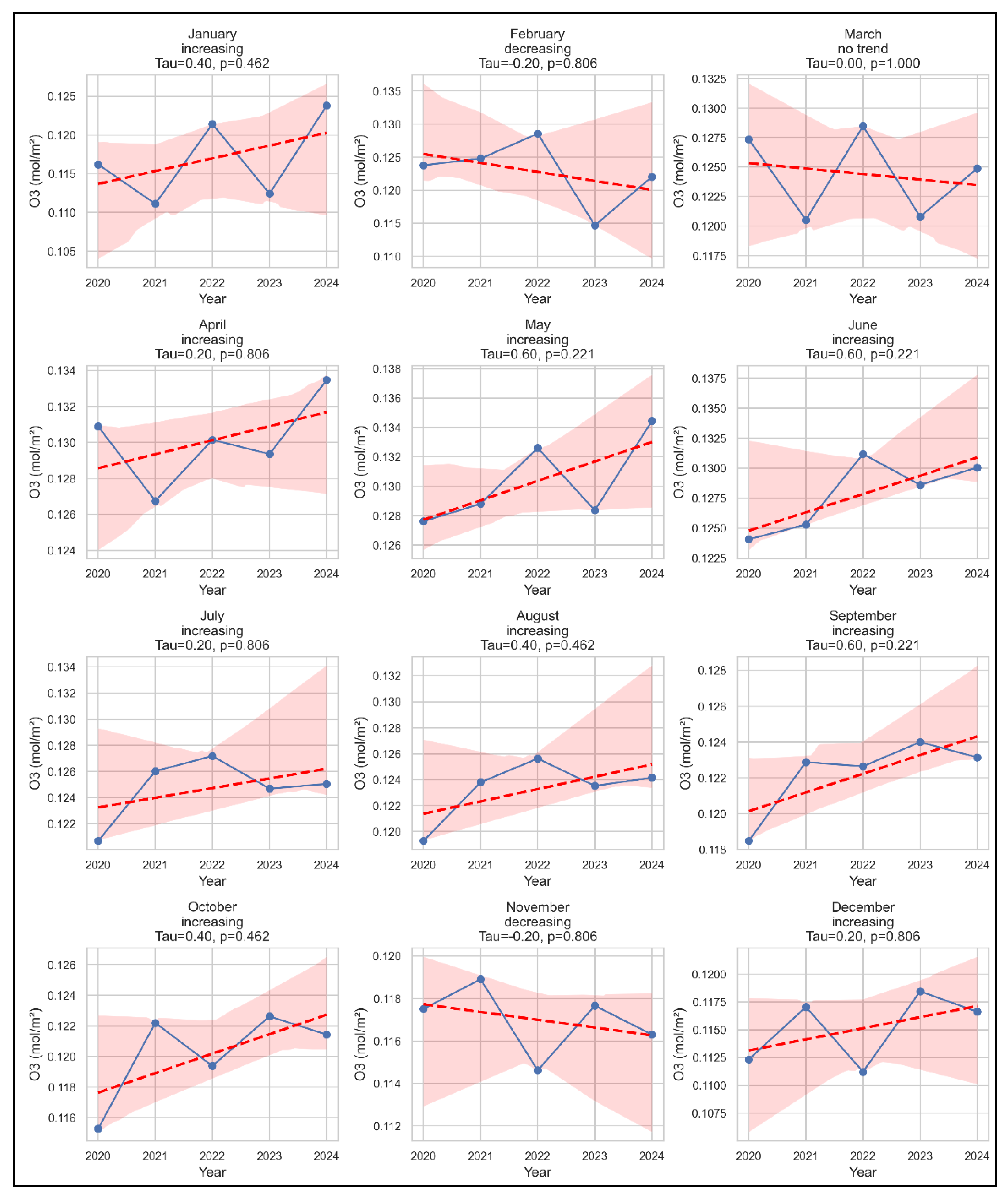
As shown in Figure 11, O₃ trends were predominantly positive throughout the year. Months such as May, June, and September showed moderate increasing tendencies (Tau = 0.6; p = 0.220), while January, August, and October had moderate upward trends as well (Tau = 0.4; p = 0.462). Decreasing trends were observed in February and November, but without statistical significance.
3.4. Spatial Distribution and Intra-Urban Pollution Zones
The spatial distribution of atmospheric pollutants across Dhaka City from 2020 to 2024 revealed distinct intra-urban heterogeneity that corresponded strongly with land use characteristics, emission source density, urban form, and prevailing meteorological patterns (Figure 2 to Figure 6). Zone-wise analysis of Sentinel-5P-derived data for CO, NO₂, SO₂, and O₃ demonstrated significant spatial clustering of pollutant concentrations, which was persistent across years and seasons.
The spatial pattern of CO concentrations across Dhaka indicated prominent hotspots in central-western and southern zones, particularly those encompassing Mirpur, Tejgaon, Hazaribagh, and Mohammadpur (Figure 3). The road-heavy zones with poor traffic circulation exhibited consistently elevated CO concentrations, with monthly averages frequently exceeding 0.04 mol/m² during winter months. Additionally, commercial and transportation corridors near Gabtoli and Kallyanpur showed notable CO accumulation, especially during the dry season, indicating the influence of vehicular idling and bottlenecks.
Peripheral zones, particularly in the north-eastern and eastern areas such as Badda and Bashundhara, consistently showed lower CO concentrations, likely due to relatively lower population densities, higher vegetation cover, and better dispersion conditions facilitated by proximity to open spaces and wetland patches.
NO₂ concentrations exhibited spatial clustering along high-traffic and high-density urban zones, with peak levels consistently recorded in central and northern sectors. The highest concentrations were observed in Motijheel, Farmgate, Gulshan, and Mohakhali—areas (Figure 4) that function as commercial and administrative hubs with high volumes of daily commuter traffic. The correlation between NO₂ and transportation activity was particularly strong, reflecting the dominance of vehicular exhaust as the primary emission source.
Notably, zones along the airport corridor (from Banani to Uttara) also exhibited episodic NO₂ spikes, especially during the pre-monsoon season. This may be attributed to increased aviation activity, commercial transport operations, and associated roadway emissions. Comparatively, residential zones such as Lalmatia and Shyamoli reported lower NO₂ values, suggesting that land use and traffic volume are primary spatial drivers of NO₂ variability.
The spatial distribution of SO₂ concentrations was more localized and distinctively clustered around the southern and southeastern zones of Dhaka, particularly in Keraniganj, Jatrabari, and parts of Demra (Figure 5). These areas host brick kilns, small-scale manufacturing units, and diesel-based energy generation facilities—all major sources of sulfur emissions. Seasonal SO₂ hotspots were most intense during winter and pre-monsoon periods, with monthly mean concentrations exceeding 0.0018 mol/m² in some zones.
Unlike primary pollutants, O₃ showed a distinct spatial pattern influenced by photochemical processes and regional transport mechanisms. The highest concentrations of ozone were observed in peri-urban and suburban zones, particularly in Uttara, Badda, and eastern fringe areas (Figure 6) adjacent to open and vegetated spaces.
The core urban zones, including Motijheel, Farmgate, and Tejgaon, consistently recorded lower ozone levels—an outcome likely linked to titration of O₃ by high NO concentrations in heavily polluted environments. This phenomenon, commonly known as the “ozone scavenging effect,” results in suppressed O₃ formation in NO-rich areas and elevated ozone levels in surrounding downwind zones where NO₂ photolysis occurs in the presence of sunlight and VOCs.
4. Discussion
This study revealed distinct spatiotemporal variations in the concentrations of CO, NO₂, SO₂, and O₃ across Dhaka City from 2020 to 2024, using Sentinel-5P satellite data processed through Google Earth Engine. The findings indicate that Dhaka’s air quality is strongly influenced by seasonal meteorology, anthropogenic activity patterns, and the city’s heterogeneous urban morphology. The discussion that follows interprets these patterns in terms of causes, implications, and relevance for environmental management and policy.
4.1. Temporal Variability and Seasonal Dynamics
The observed temporal patterns are consistent with known urban air pollution dynamics in tropical monsoon climates. Wintertime accumulation of CO, NO₂, and SO₂ is driven by reduced boundary layer height, thermal inversion, and elevated emissions from vehicular traffic, industrial activities, and residential combustion [4,13,25] (Figure 7). These conditions limit vertical dispersion, trapping pollutants near ground level and increasing human exposure. Elevated winter CO levels reflect intensified vehicular traffic and residential combustion of biomass and fossil fuels. NO₂ and SO₂ peaks during the same period likely result from increased energy consumption for heating, higher industrial activity, and continued operation of diesel-based generators due to erratic grid power [26].
In contrast, monsoon months (June–August) provide a cleansing effect (Figure 7), lowering pollutant levels due to rain-induced wet deposition, enhanced vertical mixing, enhanced atmospheric dispersion and reduced industrial activity [26,27] corroborating findings from previous studies in South Asian megacities [28,29,30,31,32]. This was particularly evident in the near-zero SO₂ values during July–August across all years, suggesting operational shutdowns of key SO₂ sources like brick kilns.
Ozone displayed an inverse seasonal trend, peaking during the pre-monsoon period. The spring/summer peak in O₃ (Figure 7) is attributed to intensified photochemical reactions under high solar radiation, involving precursor gases such as NOx and VOCs[33,34]. The temporal alignment of ozone maxima with NO₂ decline in April–May underscores the role of complex atmospheric chemistry, where NO₂ photolysis and low NO concentrations allow O₃ accumulation, especially in peripheral zones downwind from emission centers [35].
4.2. Spatial Heterogeneity and Urban Emission Sources
The spatial analysis uncovered significant intra-urban variation in pollutant concentrations across Dhaka’s administrative zones. These spatial disparities are largely governed by the spatial arrangement of emission sources, land use patterns, and urban microclimates.
CO hotspots in zones such as Tejgaon, Mirpur, and Mohammadpur align with areas (Figure 3) of high population density, congested traffic corridors, and unplanned residential-industrial coexistence. The correlation between traffic volume and CO levels reflects typical urban pollution signatures, where incomplete combustion in aging vehicles dominates emissions [36].
NO₂ concentrations were especially high in the commercial core and transport hubs—Motijheel, Mohakhali, and Gulshan (Figure 4)—corresponding to heavy-duty vehicular movement and idling emissions. Given NO₂’s short atmospheric lifetime and local origin, its spatial distribution serves as a direct proxy for localized transportation emissions and combustion activity [1]
SO₂ hotspots were sharply concentrated in industrial and peri-industrial zones such as Keraniganj and Jatrabari (Figure 5). These areas house numerous brick kilns and manufacturing plants that burn sulfur-rich fuels such as coal and heavy oil, releasing substantial quantities of SO₂[37]. The concentration gradients observed around these zones suggest both point-source emissions and short-range diffusion.
O₃ hotspots in downwind, peri-urban areas like Uttara and Badda (Figure 6) reflect photochemical transformation rather than direct emission. In the urban core, high NO concentrations scavenge ozone via titration, whereas peripheral zones allow for O₃ formation due to sufficient precursor presence and sunlight. This spatial pattern, supported by other studies in subtropical cities, demonstrates the complexity of managing ozone pollution, which often intensifies away from emission sources [38,39,40].
4.3. Influence of COVID-19 and Post-Pandemic Recovery
The temporal analysis suggests a marked dip in CO and NO₂ concentrations during 2020, coinciding with COVID-19 lockdown periods. The sharp reduction in vehicular traffic, industrial output, and construction activities significantly lowered atmospheric emissions [41]. However, the rebound in pollutant levels in subsequent years—especially 2022 and 2023—highlights the transience of air quality improvements in the absence of sustained emission control policies.
The data also suggest a lagged recovery in SO₂ concentrations, likely due to delayed resumption of industrial operations and energy demand fluctuations. These post-pandemic dynamics underscore the importance of integrating environmental recovery into economic revival planning.
4.4. Mann-Kendall Monthly Trend of Pollutants
The Mann-Kendall trend test applied to monthly maximum concentrations of CO, NO₂, SO₂, and O₃ from 2020 to 2024 indicated subtle but informative patterns of change, although most trends were not statistically significant (Figure 8 to Figure 11 and Table A2). Nonetheless, the directionality of trends reveals emerging dynamics in Dhaka’s urban atmosphere and reflects evolving emission behavior and seasonal variability.
CO showed predominantly increasing trends, particularly in June and September (Tau = 0.8; p = 0.086), suggesting seasonal build-up during early monsoon and post-monsoon months (Figure 8 and Table A2). These increases may be linked to vehicular emissions, biomass burning, and combustion from informal sectors under humid and stagnant atmospheric conditions. Declines observed in February, March, and winter months may reflect seasonal meteorology and temporary behavioral shifts, though not significant. Such patterns align with earlier studies showing CO elevation during periods of low dispersion and increased fuel use [4,13].
NO₂ exhibited generally decreasing trends, most notably in September (Tau = –0.6; p = 0.220), indicating possible improvements from vehicle emission control and wider CNG adoption (Figure 9 and Table A2). However, flat trends in January, April, and August suggest persistent emissions in transport corridors. The impact of pandemic-related activity reductions may also contribute to these observations [42].
SO₂ displayed the strongest upward trends, especially in April and May (Tau = 0.8; p = 0.086), consistent with pre-monsoon peaks in industrial and brick kiln activity (Figure 10 and Table A2). This is concerning, as SO₂ is a key contributor to acid rain and respiratory ailments. Slight declines in late monsoon and early winter likely reflect kiln closures and seasonal wind shifts [37].
O₃ trends were moderately positive in most months, particularly in May, June, and September (Tau = 0.6), reflecting enhanced photochemical formation under high sunlight and temperature (Figure 11 and Table A2). Peripheral zones may be more affected due to lower NOx titration and downwind transport. These findings echo regional concerns about rising tropospheric ozone in densely populated cities [43,44].
Although statistical significance was limited by the five-year time frame, the trends suggest rising concern for CO, SO₂, and O₃, while NO₂ may be stabilizing. These insights underscore the need for targeted seasonal interventions—such as stricter industrial regulation in pre-monsoon months and vehicle emission control in winter. The use of Sentinel-5P and Mann-Kendall analysis provides a replicable approach for early detection of air quality changes in data-scarce urban contexts.
4.5. Policy Relevance and Urban Planning Implications
The spatiotemporal dynamics of air pollutants in Dhaka uncovered in this study have profound implications for public health, environmental governance, and urban planning. Dhaka consistently ranks among the most polluted cities in the world, with one of the highest pollution-related mortality rates in South Asia [45]. The findings from our 60-month Sentinel-5P-based assessment underscore the urgency of adopting geographically targeted and seasonally adaptive air quality management strategies. The concentration of pollutants such as CO, NO₂, SO₂, and O₃ in specific urban zones and seasons indicates that a uniform policy approach would be inadequate. Instead, a multi-sectoral, zone-specific, and temporally nuanced intervention framework is essential for addressing the evolving challenges of air pollution in Dhaka [46,47].
Transport Policy: Our analysis identified central business districts and high-traffic corridors—such as Motijheel, Tejgaon, Farmgate, and Gabtoli—as persistent hotspots for CO and NO₂, with peak values occurring during winter months. These trends are largely driven by vehicular emissions exacerbated by thermal inversion and traffic congestion [13,42]. To mitigate these impacts, establishing low-emission zones (LEZs) in high-exposure neighborhoods should be prioritized. Policy measures could include phasing out older diesel vehicles, enforcing stricter vehicle emission standards, and incentivizing the adoption of compressed natural gas (CNG) and electric vehicles [46,48]. Furthermore, investment in reliable and efficient public transit infrastructure—including electric buses, metro rail expansions, and park-and-ride systems—would reduce dependency on private and informal transport modes. Congestion pricing and intelligent traffic management in these identified zones could further alleviate air quality burdens during high-emission periods [48,49].
Industrial Regulation: The spatial clustering of SO₂ concentrations around southern and southeastern industrial belts—particularly in Jatrabari, Demra, and Keraniganj—indicates the dominance of stationary sources such as brick kilns, small-scale manufacturing units, and diesel-fired generators. Our data revealed peak SO₂ levels in the pre-monsoon and winter seasons, with monthly maxima exceeding 0.00043 mol/m². These findings support the urgent need for targeted industrial regulation. Fuel switching—from coal and diesel to LPG or electricity—must be prioritized in brick kiln operations and informal industries [49,50]. Introducing clean production technologies, enforcing stack emission standards, and relocating high-emission industries away from residential clusters through better zoning practices are essential steps. Integration of emissions monitoring into building permits and environmental clearance processes can also ensure long-term compliance and transparency [51]
Ozone Control: Unlike primary pollutants, O₃ exhibited an inverse seasonal pattern, peaking during the pre-monsoon months with concentrations exceeding 0.130 mol/m² in May. High ozone levels were recorded in peri-urban zones such as Uttara and Badda, driven by photochemical reactions involving transported NOx and VOCs in sunlight-rich conditions[34,50]. Ozone mitigation, therefore, requires an indirect yet strategic approach. This includes controlling both NOx and VOC emissions from transport and industrial solvents, regulating fuel composition, and promoting vapor recovery systems in fueling stations. Expanding urban green cover in ozone-sensitive downwind zones may also contribute to natural filtration and dispersion, while offering additional climate resilience and public health co-benefits[52]. Interventions must account for the ozone scavenging effect observed in core urban areas with high NO emissions, which paradoxically lowers O₃ concentrations locally but amplifies regional ozone burdens [43]
Zonal Monitoring and Data-Driven Governance: The pronounced intra-urban variability revealed by Sentinel-5P TROPOMI data illustrates the inadequacy of current ground-based air quality monitoring networks, which often lack spatial granularity and temporal continuity ([21,31]. The use of satellite remote sensing and Google Earth Engine [9] in this study provides a scalable, cloud-based, and cost-effective framework for generating zone-specific air pollution baselines. These baselines can inform dynamic and adaptive environmental governance policies. Institutionalizing such monitoring frameworks within city governance systems (e.g., Dhaka North and South City Corporations) can facilitate real-time data integration into urban planning decisions. Additionally, integrating Sentinel-derived air quality layers with socio-economic and health datasets could enable targeted interventions in vulnerable neighborhoods, thereby maximizing the impact of environmental policies on human well-being.
Policy Integration and Institutional Coordination: A key insight from this study is the interdependence between various pollution sources and their spatial-temporal impacts. Thus, policy responses must be integrative rather than fragmented. Coordination between urban planning authorities, environmental regulatory bodies, transportation departments, and health agencies is crucial. Establishing an interagency urban air quality task force could ensure alignment across sectoral policies and enhance the implementation of evidence-based strategies [32,42]. Furthermore, periodic updates of zoning regulations, informed by remote sensing data, can help balance development and environmental objectives.
5. Conclusions
This study provides a comprehensive assessment of the spatiotemporal behavior of four key atmospheric pollutants—CO, NO₂, SO₂, and O₃—across Dhaka City over a five-year period (2020–2024) using Sentinel-5P satellite imagery and cloud-based analysis via Google Earth Engine. The results revealed strong seasonal variability and spatial heterogeneity in pollutant concentrations, reflecting the interplay of emission sources, land use, and meteorological conditions. CO, NO₂, and SO₂ concentrations peaked in winter due to enhanced combustion activities and poor dispersion, while O₃ levels reached maximum during pre-monsoon months due to favorable photochemical conditions. Spatial patterns showed persistent pollution hotspots aligned with traffic corridors and industrial zones, while ozone exhibited elevated concentrations in peripheral, downwind areas due to titration effects.
Trend analysis using the Mann-Kendall test showed increasing tendencies in CO, SO₂, and O₃ levels across several months, though most trends were not statistically significant given the limited temporal span. Nevertheless, these results indicate emerging concerns regarding pollution accumulation and underscore the importance of seasonal and zone-specific mitigation efforts. The integration of satellite remote sensing and cloud-based geospatial platforms proved effective in generating high-resolution, long-term air quality assessments, offering a replicable framework for similar cities facing monitoring constraints. These insights can inform evidence-based urban planning, emission control policies, and adaptive air quality management strategies tailored to Dhaka’s evolving urban landscape.
Author Contributions
Conceptualization, M.M.R.; methodology M.M.R.; software, M.M.R., M.I.F, and M.K.Z.; validation, M.M.R.; formal analysis, M.M.R., M.K.Z and M.I.F; investigation, M.M.R.; resources, M.K.Z and M.I.F.; data curation, M.M.R.; writing—original draft preparation, M.M.R., M.K.Z and M.I.F; writing—review and editing, M.M.R. and G.S.; visualization, M.M.R.; supervision, G.S.; project administration, M.M.R. All authors have read and agreed to the published version of the manuscript.
Funding
This research was funded by Rajshahi University of Engineering & Technology (RUET), grant number DRE/8/RUET/700/(66)/pro/2024-2025/16.
Data Availability Statement
The datasets used in this study are available from the corresponding author on request.
Acknowledgments
We gratefully acknowledge the European Space Agency (ESA) for providing free access to Sentinel-5P TROPOMI satellite imagery through the Copernicus Programme, which served as the primary data source for this study. The analysis was conducted using the cloud-based Google Earth Engine (GEE). This open-access platforms and tools were instrumental in enabling the spatiotemporal assessment and hotspot analysis of urban air pollutants in Dhaka City.
Conflicts of Interest
The authors declare no conflicts of interest.
Abbreviations
The following abbreviations are used in this manuscript:
| CO | Carbon Monoxide |
| GEE | Google Earth Engine |
| NO₂ | Nitrogen Dioxide |
| O₃ | Ozone |
| OSM | Open Street Map |
| QA | Quality Assurance |
| SO₂ | Sulfur Dioxide |
| TROPOMI | Tropospheric Monitoring Instrument |
| UTM | Universal Transverse Mercator |
| WGS | World Geodetic System |
| WHO | World Health Organization |
Appendix A

Table A1.
Monthly average pollution concentration (mol/m2) (2020-2024).
| Pollutant | Month | Mean | Min | Max | StdDev |
| CO | Jan | 0.0513614 | 0.0496658 | 0.0528690 | 0.0006383 |
| CO | Feb | 0.0503589 | 0.0493792 | 0.0510958 | 0.0003252 |
| CO | Mar | 0.0517501 | 0.0504490 | 0.0530655 | 0.0004845 |
| CO | Apr | 0.0501786 | 0.0491893 | 0.0512107 | 0.0004769 |
| CO | May | 0.0463520 | 0.0457516 | 0.0471837 | 0.0002862 |
| CO | Jun | 0.0421077 | 0.0414376 | 0.0429054 | 0.0002888 |
| CO | Jul | 0.0336378 | 0.0327860 | 0.0343351 | 0.0003111 |
| CO | Aug | 0.0349084 | 0.0340728 | 0.0355727 | 0.0003255 |
| CO | Sep | 0.0370318 | 0.0362062 | 0.0375760 | 0.0002866 |
| CO | Oct | 0.0405656 | 0.0397436 | 0.0415074 | 0.0003488 |
| CO | Nov | 0.0445893 | 0.0431804 | 0.0453095 | 0.0004129 |
| CO | Dec | 0.0491688 | 0.0470178 | 0.0503863 | 0.0006701 |
| NO2 | Jan | 0.0003024 | 0.0002214 | 0.0003538 | 0.0000220 |
| NO2 | Feb | 0.0002512 | 0.0001832 | 0.0002996 | 0.0000192 |
| NO2 | Mar | 0.0002500 | 0.0001758 | 0.0003157 | 0.0000298 |
| NO2 | Apr | 0.0001171 | 0.0000753 | 0.0001521 | 0.0000137 |
| NO2 | May | 0.0001249 | 0.0000915 | 0.0001747 | 0.0000153 |
| NO2 | Jun | 0.0000914 | 0.0000561 | 0.0001220 | 0.0000123 |
| NO2 | Jul | 0.0000813 | 0.0000528 | 0.0001025 | 0.0000100 |
| NO2 | Aug | 0.0000827 | 0.0000563 | 0.0001006 | 0.0000091 |
| NO2 | Sep | 0.0001221 | 0.0000825 | 0.0001502 | 0.0000139 |
| NO2 | Oct | 0.0001870 | 0.0001296 | 0.0002367 | 0.0000174 |
| NO2 | Nov | 0.0002505 | 0.0001754 | 0.0003057 | 0.0000286 |
| NO2 | Dec | 0.0002861 | 0.0002124 | 0.0003477 | 0.0000266 |
| O3 | Jan | 0.1166113 | 0.1163946 | 0.1167787 | 0.0000739 |
| O3 | Feb | 0.1223674 | 0.1221601 | 0.1226222 | 0.0001024 |
| O3 | Mar | 0.1240289 | 0.1237723 | 0.1242836 | 0.0001006 |
| O3 | Apr | 0.1298555 | 0.1297234 | 0.1299784 | 0.0000632 |
| O3 | May | 0.1300368 | 0.1298265 | 0.1302312 | 0.0000822 |
| O3 | Jun | 0.1274474 | 0.1273492 | 0.1276508 | 0.0000450 |
| O3 | Jul | 0.1243732 | 0.1240519 | 0.1245990 | 0.0000839 |
| O3 | Aug | 0.1229746 | 0.1228815 | 0.1231112 | 0.0000436 |
| O3 | Sep | 0.1219184 | 0.1217339 | 0.1220841 | 0.0000615 |
| O3 | Oct | 0.1198456 | 0.1197089 | 0.1200084 | 0.0000644 |
| O3 | Nov | 0.1167096 | 0.1165568 | 0.1168116 | 0.0000472 |
| O3 | Dec | 0.1147646 | 0.1146131 | 0.1150170 | 0.0000667 |
| SO2 | Jan | 0.0002467 | 0.0000471 | 0.0004135 | 0.0000644 |
| SO2 | Feb | 0.0002999 | 0.0001972 | 0.0004326 | 0.0000407 |
| SO2 | Mar | 0.0002985 | 0.0002017 | 0.0004080 | 0.0000384 |
| SO2 | Apr | 0.0002144 | 0.0001565 | 0.0002967 | 0.0000241 |
| SO2 | May | 0.0000787 | 0.0000104 | 0.0001880 | 0.0000337 |
| SO2 | Jun | 0.0000584 | 0.0000000 | 0.0001419 | 0.0000329 |
| SO2 | Jul | 0.0000286 | 0.0000000 | 0.0001090 | 0.0000266 |
| SO2 | Aug | 0.0000379 | 0.0000000 | 0.0001342 | 0.0000288 |
| SO2 | Sep | 0.0000580 | 0.0000000 | 0.0001786 | 0.0000321 |
| SO2 | Oct | 0.0000717 | 0.0000153 | 0.0001525 | 0.0000263 |
| SO2 | Nov | 0.0001026 | 0.0000000 | 0.0002382 | 0.0000580 |
| SO2 | Dec | 0.0001576 | 0.0000369 | 0.0003072 | 0.0000560 |
Table A2.
Man-Kendal test of monthly maximum pollutants concentration (2020-2024).
| Pollutant | Month | Trend | Tau | P-value |
| CO | Jan | increasing | 0.2 | 0.806495941 |
| CO | Feb | decreasing | -0.2 | 0.806495941 |
| CO | Mar | decreasing | -0.2 | 0.806495941 |
| CO | Apr | increasing | 0.4 | 0.462432726 |
| CO | May | increasing | 0.4 | 0.462432726 |
| CO | Jun | increasing | 0.8 | 0.086410733 |
| CO | Jul | increasing | 0.2 | 0.806495941 |
| CO | Aug | increasing | 0.4 | 0.462432726 |
| CO | Sep | increasing | 0.8 | 0.086410733 |
| CO | Oct | increasing | 0.2 | 0.806495941 |
| CO | Nov | decreasing | -0.2 | 0.806495941 |
| CO | Dec | decreasing | -0.2 | 0.806495941 |
| NO2 | Jan | no trend | 0 | 1 |
| NO2 | Feb | decreasing | -0.4 | 0.462432726 |
| NO2 | Mar | decreasing | -0.2 | 0.806495941 |
| NO2 | Apr | no trend | 0 | 1 |
| NO2 | May | increasing | 0.2 | 0.806495941 |
| NO2 | Jun | increasing | 0.4 | 0.462432726 |
| NO2 | Jul | decreasing | -0.2 | 0.806495941 |
| NO2 | Aug | no trend | 0 | 1 |
| NO2 | Sep | decreasing | -0.6 | 0.220671362 |
| NO2 | Oct | decreasing | -0.4 | 0.462432726 |
| NO2 | Nov | decreasing | -0.4 | 0.462432726 |
| NO2 | Dec | decreasing | -0.4 | 0.462432726 |
| O3 | Jan | increasing | 0.4 | 0.462432726 |
| O3 | Feb | decreasing | -0.2 | 0.806495941 |
| O3 | Mar | no trend | 0 | 1 |
| O3 | Apr | increasing | 0.2 | 0.806495941 |
| O3 | May | increasing | 0.6 | 0.220671362 |
| O3 | Jun | increasing | 0.6 | 0.220671362 |
| O3 | Jul | increasing | 0.2 | 0.806495941 |
| O3 | Aug | increasing | 0.4 | 0.462432726 |
| O3 | Sep | increasing | 0.6 | 0.220671362 |
| O3 | Oct | increasing | 0.4 | 0.462432726 |
| O3 | Nov | decreasing | -0.2 | 0.806495941 |
| O3 | Dec | increasing | 0.2 | 0.806495941 |
| SO2 | Jan | no trend | 0 | 1 |
| SO2 | Feb | no trend | 0 | 1 |
| SO2 | Mar | increasing | 0.2 | 0.806495941 |
| SO2 | Apr | increasing | 0.8 | 0.086410733 |
| SO2 | May | increasing | 0.8 | 0.086410733 |
| SO2 | Jun | no trend | 0 | 1 |
| SO2 | Jul | increasing | 0.2 | 0.806495941 |
| SO2 | Aug | decreasing | -0.2 | 0.806495941 |
| SO2 | Sep | decreasing | -0.4 | 0.462432726 |
| SO2 | Oct | no trend | 0 | 1 |
| SO2 | Nov | decreasing | -0.4 | 0.462432726 |
| SO2 | Dec | decreasing | -0.4 | 0.462432726 |
References
- Goshua, A.; Akdis, C.A.; Nadeau, K.C. World Health Organization Global Air Quality Guideline Recommendations: Executive Summary. Allergy: European Journal of Allergy and Clinical Immunology 2022, 77. [CrossRef]
- Kampa, M.; Castanas, E. Human Health Effects of Air Pollution. Environmental Pollution 2008, 151. [CrossRef]
- Anderson, J.O.; Thundiyil, J.G.; Stolbach, A. Clearing the Air: A Review of the Effects of Particulate Matter Air Pollution on Human Health. Journal of Medical Toxicology 2012, 8. [CrossRef]
- Gurjar, B.R.; Jain, A.; Sharma, A.; Agarwal, A.; Gupta, P.; Nagpure, A.S.; Lelieveld, J. Human Health Risks in Megacities Due to Air Pollution. Atmos Environ 2010, 44. [CrossRef]
- IQAir World Air Quality Report 2024; 2024;
- Zahangeer Alam, M.; Armin, E.; Haque, M.M.; Halsey, J.; Qayum, Md.A. Air Pollutants and Their Possible Health Effects at Different Locations in Dhaka City. Journal of Current Chemical and Pharmaceutical Sciences 2018, 08. [CrossRef]
- Ali, M.E.; Hasan, M.F.; Siddiqa, S.; Molla, M.M.; Nasrin Akhter, M. FVM-RANS Modeling of Air Pollutants Dispersion and Traffic Emission in Dhaka City on a Suburb Scale. Sustainability (Switzerland) 2023, 15. [CrossRef]
- Veefkind, J.P.; Aben, I.; McMullan, K.; Förster, H.; de Vries, J.; Otter, G.; Claas, J.; Eskes, H.J.; de Haan, J.F.; Kleipool, Q.; et al. TROPOMI on the ESA Sentinel-5 Precursor: A GMES Mission for Global Observations of the Atmospheric Composition for Climate, Air Quality and Ozone Layer Applications. Remote Sens Environ 2012, 120. [CrossRef]
- Gorelick, N.; Hancher, M.; Dixon, M.; Ilyushchenko, S.; Thau, D.; Moore, R. Google Earth Engine: Planetary-Scale Geospatial Analysis for Everyone. Remote Sens Environ 2017, 202. [CrossRef]
- Bauwens, M.; Compernolle, S.; Stavrakou, T.; Müller, J.F.; van Gent, J.; Eskes, H.; Levelt, P.F.; van der A, R.; Veefkind, J.P.; Vlietinck, J.; et al. Impact of Coronavirus Outbreak on NO2 Pollution Assessed Using TROPOMI and OMI Observations. Geophys Res Lett 2020, 47. [CrossRef]
- Matandirotya, N.R.; Burger, R.P. Spatiotemporal Variability of Tropospheric NO2 over Four Megacities in Southern Africa: Implications for Transboundary Regional Air Pollution. Environmental Challenges 2021, 5. [CrossRef]
- Biswas, A.; Modak, N. A Multiobjective Fuzzy Chance Constrained Programming Model for Land Allocation in Agricultural Sector: A Case Study. International Journal of Computational Intelligence Systems 2017. [CrossRef]
- Begum, B.A.; Biswas, S.K.; Hopke, P.K. Key Issues in Controlling Air Pollutants in Dhaka, Bangladesh. In Proceedings of the Atmospheric Environment; 2011; Vol. 45. [CrossRef]
- Nahrin, K. Environmental Area Conservation through Urban Planning: Case Study in Dhaka. Journal of Property, Planning and Environmental Law 2020. [CrossRef]
- Ahmed, S.J.; Nahiduzzaman, K.M.; Bramley, G. From a Town to a Megacity: 400 Years of Growth. In Dhaka Megacity: Geospatial Perspectives on Urbanisation, Environment and Health; 2014 ISBN 9789400767355.
- Noorunnahar, M.; Hossain, M. Trend Analysis of Rainfall Data in Divisional Meteorological Stations of Bangladesh. Annals of Bangladesh Agriculture 2020. [CrossRef]
- Bodah, B.W.; Neckel, A.; Stolfo Maculan, L.; Milanes, C.B.; Korcelski, C.; Ramírez, O.; Mendez-Espinosa, J.F.; Bodah, E.T.; Oliveira, M.L.S. Sentinel-5P TROPOMI Satellite Application for NO2 and CO Studies Aiming at Environmental Valuation. J Clean Prod 2022, 357. [CrossRef]
- Apituley, A.; Pedergnana, M.; Sneep, M.; Veefkind, J.P.; Loyola, D.; Wang, P. Sentinel-5 Precursor/TROPOMI Level 2 Product User Manual KNMI Level Support Products. S5p/TROPOMI 2018.
- Zheng, B.; Geng, G.; Ciais, P.; Davis, S.J.; Martin, R. V.; Meng, J.; Wu, N.; Chevallier, F.; Broquet, G.; Boersma, F.; et al. Satellite-Based Estimates of Decline and Rebound in China’s CO2 Emissions during COVID-19 Pandemic. Sci Adv 2020, 6. [CrossRef]
- Griffin, D.; Zhao, X.; McLinden, C.A.; Boersma, F.; Bourassa, A.; Dammers, E.; Degenstein, D.; Eskes, H.; Fehr, L.; Fioletov, V.; et al. High-Resolution Mapping of Nitrogen Dioxide With TROPOMI: First Results and Validation Over the Canadian Oil Sands. Geophys Res Lett 2019, 46. [CrossRef]
- Rahman, M.M.; Mahamud, S.; Thurston, G.D. Recent Spatial Gradients and Time Trends in Dhaka, Bangladesh, Air Pollution and Their Human Health Implications. J Air Waste Manage Assoc 2019, 69. [CrossRef]
- Ackom, E.K.; Adjei, K.A.; Odai, S.N. Spatio-Temporal Rainfall Trend and Homogeneity Analysis in Flood Prone Area: Case Study of Odaw River Basin-Ghana. SN Appl Sci 2020, 2. [CrossRef]
- Masood, M.U.; Haider, S.; Rashid, M.; Naseer, W.; Pande, C.B.; Đurin, B.; Alshehri, F.; Elkhrachy, I. Assessment of Hydrological Response to Climatic Variables over the Hindu Kush Mountains, South Asia. Water (Switzerland) 2023, 15. [CrossRef]
- Dahunsi, A.M.; Bonou, F.; Dada, O.A.; Baloïtcha, E. Spatio-Temporal Trend of Past and Future Extreme Wave Climates in the Gulf of Guinea Driven by Climate Change. J Mar Sci Eng 2022, 10. [CrossRef]
- Singh, R.P.; Chauhan, A. Sources of Atmospheric Pollution in India. In Asian Atmospheric Pollution: Sources, Characteristics and Impacts; 2021. [CrossRef]
- Anindita Saha; George R. Engelhardt; Digby D. Macdonald; Ruhul A. Khan Industrial Pollution and Its Effect in the Context of Bangladesh. World Journal of Advanced Research and Reviews 2023, 18. [CrossRef]
- Akteruzzaman, M.; Rahman, M.A.; Rabbi, F.M.; Asharof, S.; Rofi, M.M.; Hasan, M.K.; Muktadir Islam, M.A.; Khan, M.A.R.; Rahman, M.M.; Rahaman, M.H. The Impacts of Cooking and Indoor Air Quality Assessment in the Southwestern Region of Bangladesh. Heliyon 2023, 9. [CrossRef]
- Shammi, M.; Rahman, M.M.; Tareq, S.M. Distribution of Bioaerosols in Association With Particulate Matter: A Review on Emerging Public Health Threat in Asian Megacities. Front Environ Sci 2021, 9. [CrossRef]
- Majeed, R.; Anjum, M.S.; Imad-ud-din, M.; Malik, S.; Anwar, M.N.; Anwar, B.; Khokhar, M.F. Solving the Mysteries of Lahore Smog: The Fifth Season in the Country. Frontiers in Sustainable Cities 2023, 5. [CrossRef]
- Yin, X.; Kang, S.; Rupakheti, M.; de Foy, B.; Li, P.; Yang, J.; Wu, K.; Zhang, Q.; Rupakheti, D. Influence of Transboundary Air Pollution on Air Quality in Southwestern China. Geoscience Frontiers 2021, 12. [CrossRef]
- Islam, N.; Toha, T.R.; Islam, M.M.; Ahmed, T. The Association between Particulate Matter Concentration and Meteorological Parameters in Dhaka, Bangladesh. Meteorology and Atmospheric Physics 2022, 134. [CrossRef]
- Kayes, I.; Shahriar, S.A.; Hasan, K.; Akhter, M.; Kabir, M.M.; Salam, M.A. The Relationships between Meteorological Parameters and Air Pollutants in an Urban Environment. Global Journal of Environmental Science and Management 2019, 5. [CrossRef]
- Wang, T.; Xue, L.; Brimblecombe, P.; Lam, Y.F.; Li, L.; Zhang, L. Ozone Pollution in China: A Review of Concentrations, Meteorological Influences, Chemical Precursors, and Effects. Science of the Total Environment 2017, 575. [CrossRef]
- Monks, P.S.; Archibald, A.T.; Colette, A.; Cooper, O.; Coyle, M.; Derwent, R.; Fowler, D.; Granier, C.; Law, K.S.; Mills, G.E.; et al. Tropospheric Ozone and Its Precursors from the Urban to the Global Scale from Air Quality to Short-Lived Climate Forcer. Atmos Chem Phys 2015, 15. [CrossRef]
- Frey, H.C.; Grieshop, A.P.; Khlystov, A.; Bang, J.J.; Rouphail, N.; Guinness, J.; Rodriguez, D.; Fuentes, M.; Saha, P.; Brantley, H.; et al. Characterizing Determinants of Near-Road Ambient Air Quality for an Urban Intersection and a Freeway Site. Res Rep Health Eff Inst 2022.
- Juneja Gandhi, T.; Garg, P.R.; Kurian, K.; Bjurgert, J.; Sahariah, S.A.; Mehra, S.; Vishwakarma, G. Outdoor Physical Activity in an Air Polluted Environment and Its Effect on the Cardiovascular System—A Systematic Review. Int J Environ Res Public Health 2022, 19. [CrossRef]
- Majumder, A.K.; Nayeem, A. Al; Patoary, M.N.A.; Carter, W.S. Temporal Variation of Ambient Particulate Matter in Chattogram City, Bangladesh. Journal of Air Pollution and Health 2020, 5. [CrossRef]
- Sarkar, S.; Chauhan, A.; Kumar, R. Impact of Deadly Dust Storms (May 2018) on Air Quality, Meteorological, and Atmospheric Parameters Over the Northern Parts of India. Geohealth 2019, 3. [CrossRef]
- Chattopadhyay, S.; Gupta, S.; Saha, R.N. Spatial and Temporal Variation of Urban Air Quality: A GIS Approach. J Environ Prot (Irvine, Calif) 2010, 01. [CrossRef]
- Zhao, C.; Wang, Y.; Yang, Q.; Fu, R.; Cunnold, D.; Choi, Y. Impact of East Asian Summer Monsoon on the Air Quality over China: View from Space. Journal of Geophysical Research Atmospheres 2010, 115. [CrossRef]
- Islam, M.S.; Tusher, T.R.; Roy, S.; Rahman, M. Impacts of Nationwide Lockdown Due to COVID-19 Outbreak on Air Quality in Bangladesh: A Spatiotemporal Analysis. Air Qual Atmos Health 2021, 14. [CrossRef]
- Dewan, A.M.; Kabir, M.H.; Nahar, K.; Rahman, M.Z. Urbanisation and Environmental Degradation in Dhaka Metropolitan Area of Bangladesh. International Journal of Environment and Sustainable Development 2012. [CrossRef]
- Chowdhury, S.; Pillarisetti, A.; Oberholzer, A.; Jetter, J.; Mitchell, J.; Cappuccilli, E.; Aamaas, B.; Aunan, K.; Pozzer, A.; Alexander, D. A Global Review of the State of the Evidence of Household Air Pollution’s Contribution to Ambient Fine Particulate Matter and Their Related Health Impacts. Environ Int 2023, 173. [CrossRef]
- Lelieveld, J.; Evans, J.S.; Fnais, M.; Giannadaki, D.; Pozzer, A. The Contribution of Outdoor Air Pollution Sources to Premature Mortality on a Global Scale. Nature 2015, 525. [CrossRef]
- Health Effects Institute State of Global Air 2020. A Special Report on Global Exposure to Air Pollution and Its Health Impacts.; 2020;
- Sokhi, R.S.; Singh, V.; Querol, X.; Finardi, S.; Targino, A.C.; Andrade, M. de F.; Pavlovic, R.; Garland, R.M.; Massagué, J.; Kong, S.; et al. A Global Observational Analysis to Understand Changes in Air Quality during Exceptionally Low Anthropogenic Emission Conditions. Environ Int 2021, 157. [CrossRef]
- Cervero, R. Linking Urban Transport and Land Use in Developing Countries. J Transp Land Use 2013. [CrossRef]
- Loo, L.Y. Le; Corcoran, J.; Mateo-Babiano, D.; Zahnow, R. Transport Mode Choice in South East Asia: Investigating the Relationship between Transport Users’ Perception and Travel Behaviour in Johor Bahru, Malaysia. J Transp Geogr 2015, 46. [CrossRef]
- Ahmed, A.; Bin Ali, A.A.; Mahboob, M.; Humaira, F. Comparison between Local and Global Methods to Develop AQI in Representing the Spatial Pattern of Air Quality of Dhaka City. The Dhaka University Journal of Earth and Environmental Sciences 2023, 11. [CrossRef]
- Shahrukh, S.; Hossain, S.A.; Huda, M.N.; Moniruzzaman, M.; Islam, M.M.; Shaikh, M.A.A.; Hossain, M.E. Air Pollution Tolerance, Anticipated Performance, and Metal Accumulation Indices of Four Evergreen Tree Species in Dhaka, Bangladesh. Curr Plant Biol 2023, 35–36. [CrossRef]
- Kuylenstierna, J.C.I.; Heaps, C.G.; Ahmed, T.; Vallack, H.W.; Hicks, W.K.; Ashmore, M.R.; Malley, C.S.; Wang, G.; Lefèvre, E.N.; Anenberg, S.C.; et al. Development of the Low Emissions Analysis Platform – Integrated Benefits Calculator (LEAP-IBC) Tool to Assess Air Quality and Climate Co-Benefits: Application for Bangladesh. Environ Int 2020, 145. [CrossRef]
- Royal Society Ground-Level Ozone in the 21st Century: Future Trends, Impacts and Policy Implications; 2008;
Figure 1.
Location of (a) Dhaka district in Bangladesh; (b) the city of Dhaka in Dhaka district; and (c) base map of the city of Dhaka.
Figure 1.
Location of (a) Dhaka district in Bangladesh; (b) the city of Dhaka in Dhaka district; and (c) base map of the city of Dhaka.
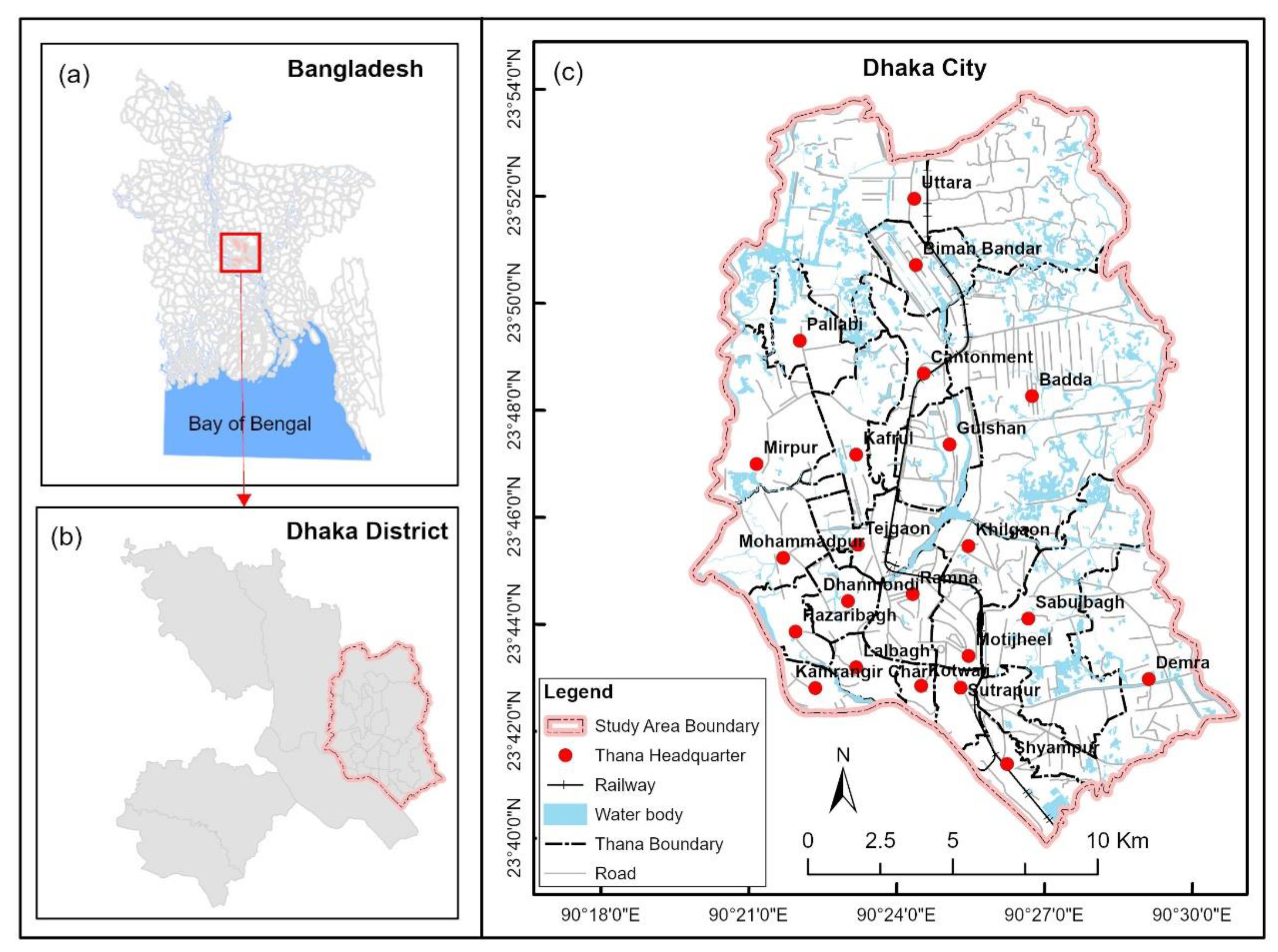
Figure 2.
Dhaka city upazila boundary.
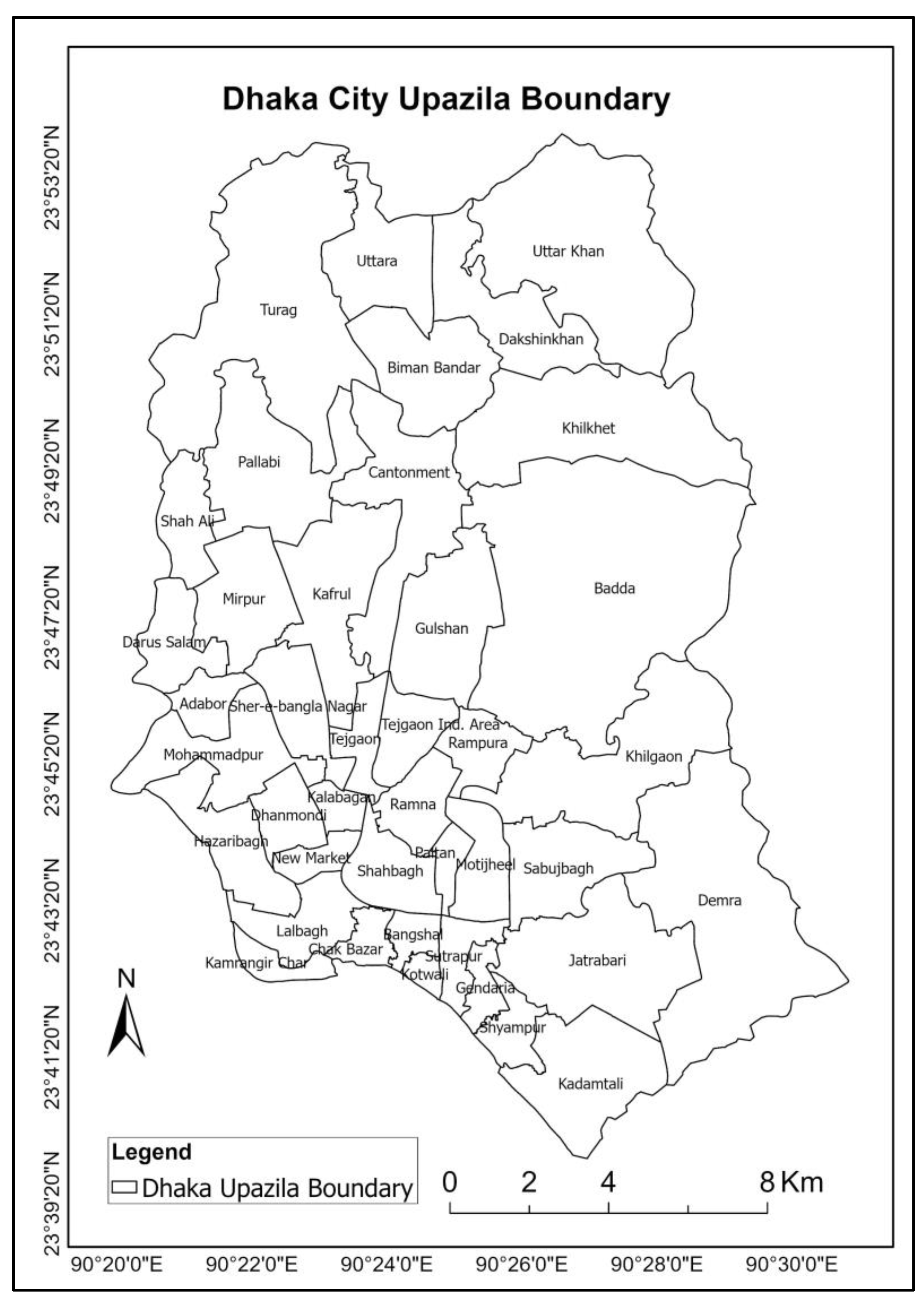
Figure 3.
Monthly average CO concentration (2020-2024) in Dhaka city.
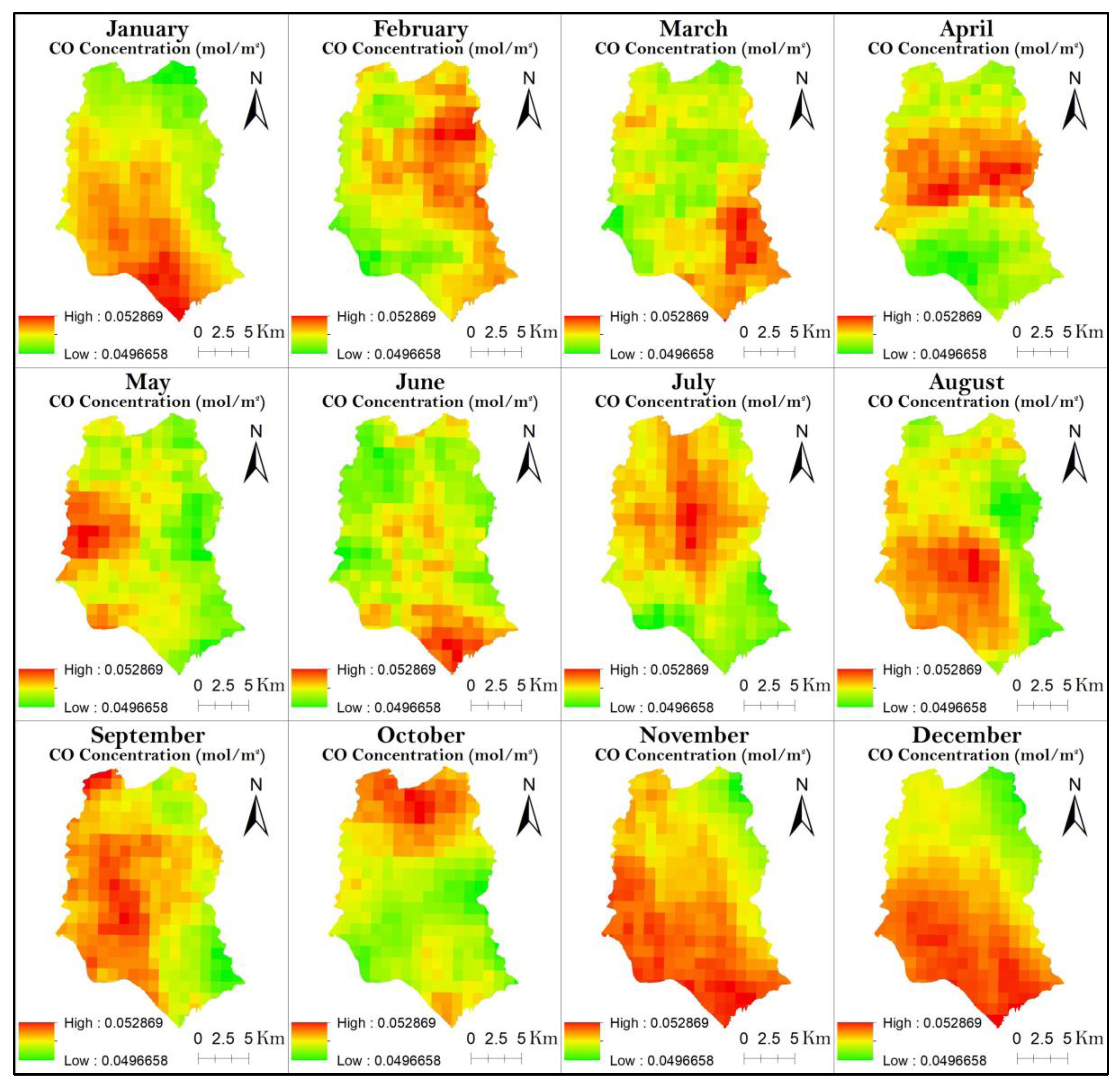
Figure 4.
Monthly average NO₂ concentration (2020-2024) in Dhaka city.
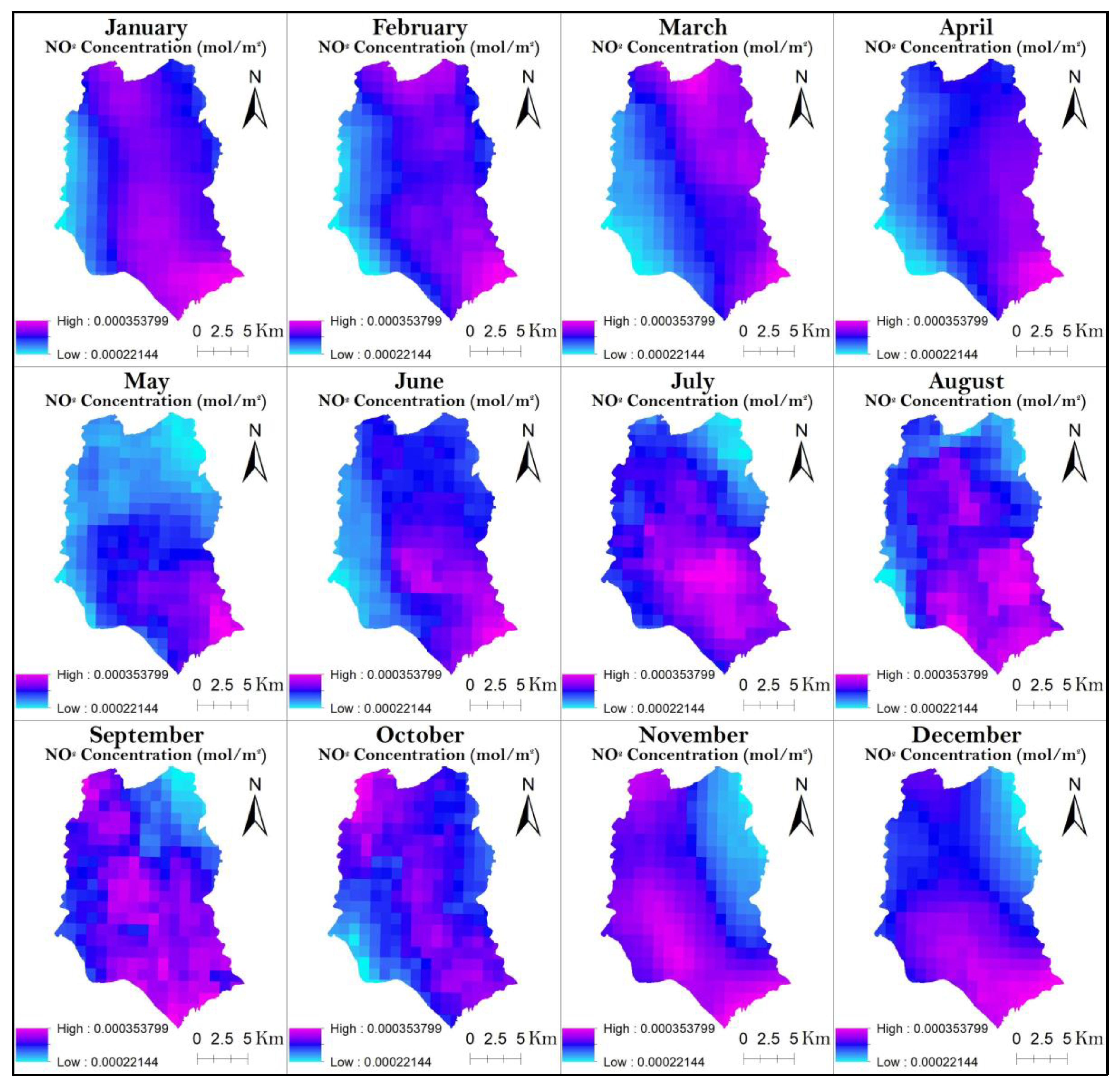
Figure 5.
Monthly average O₃ concentration (2020-2024) in Dhaka city.
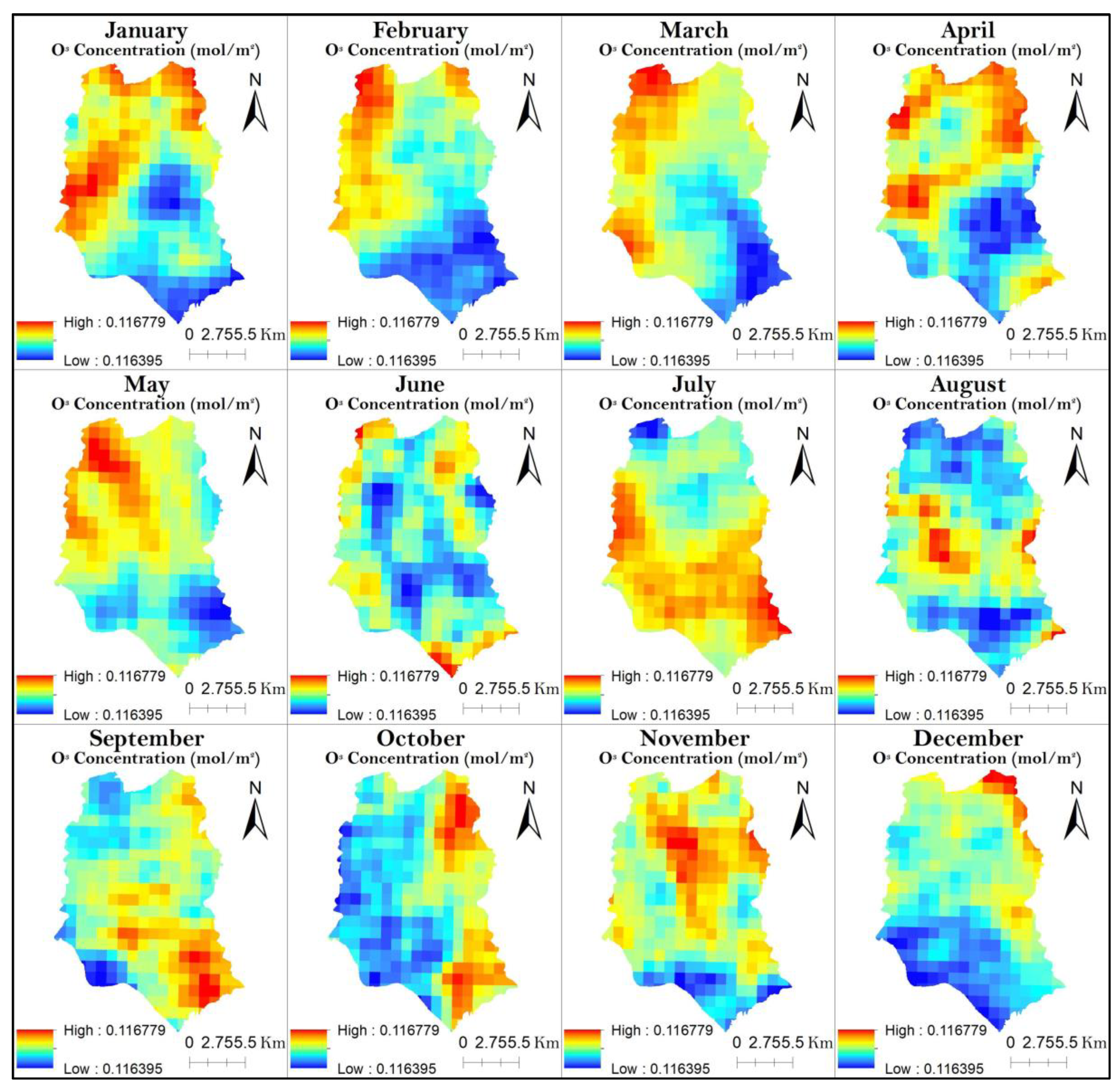
Figure 6.
Monthly average SO₂ concentration (2020-2024) in Dhaka city.
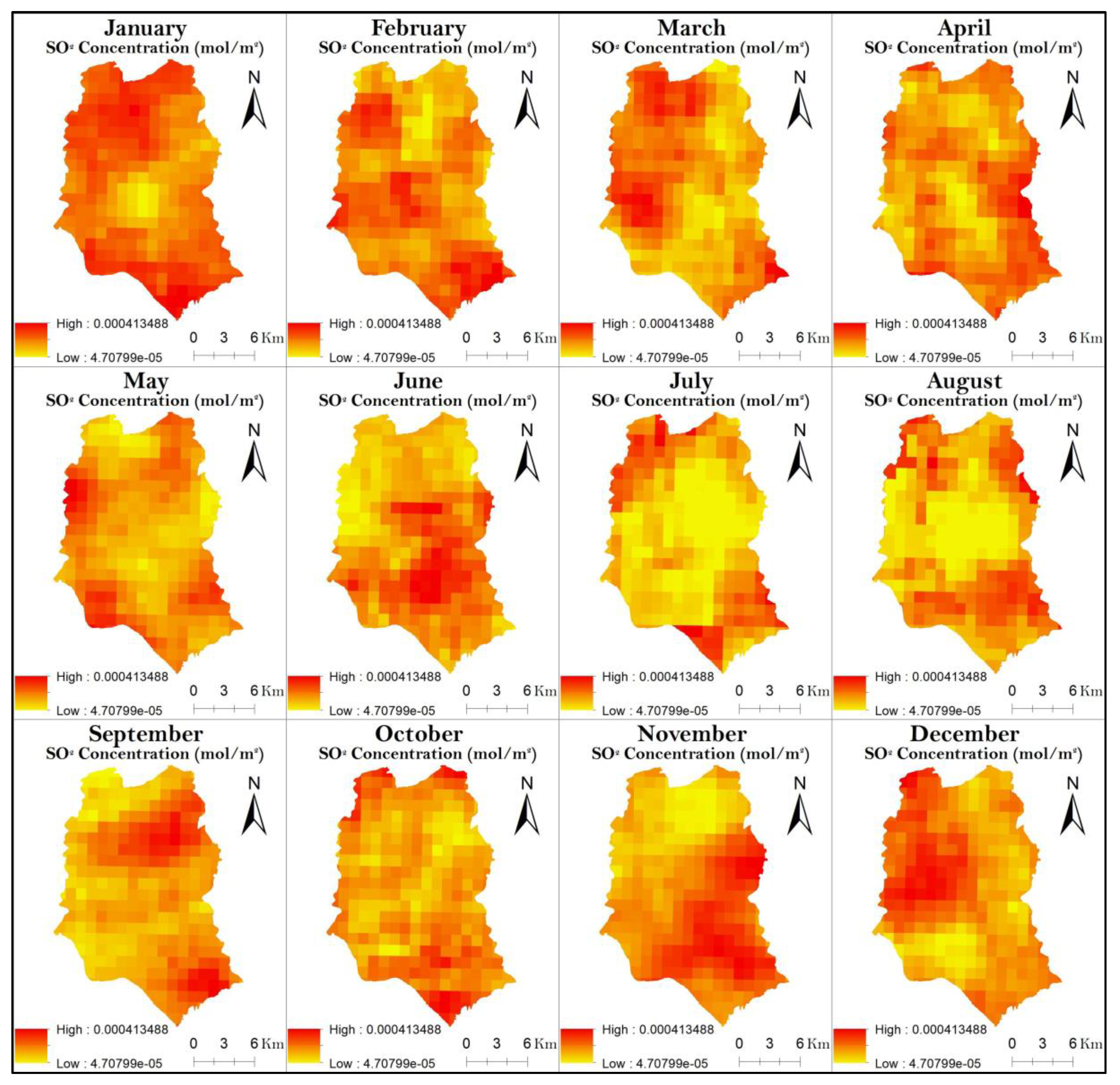
Figure 7.
Monthly average concentration trends of (a) CO, (b) NO₂, (c) SO₂, and (d) O₃ over Dhaka City from 2020 to 2024. Winter peaks in CO, NO₂, and SO₂ are consistent across years, while O₃ displays photochemical summer peaks.
Figure 7.
Monthly average concentration trends of (a) CO, (b) NO₂, (c) SO₂, and (d) O₃ over Dhaka City from 2020 to 2024. Winter peaks in CO, NO₂, and SO₂ are consistent across years, while O₃ displays photochemical summer peaks.
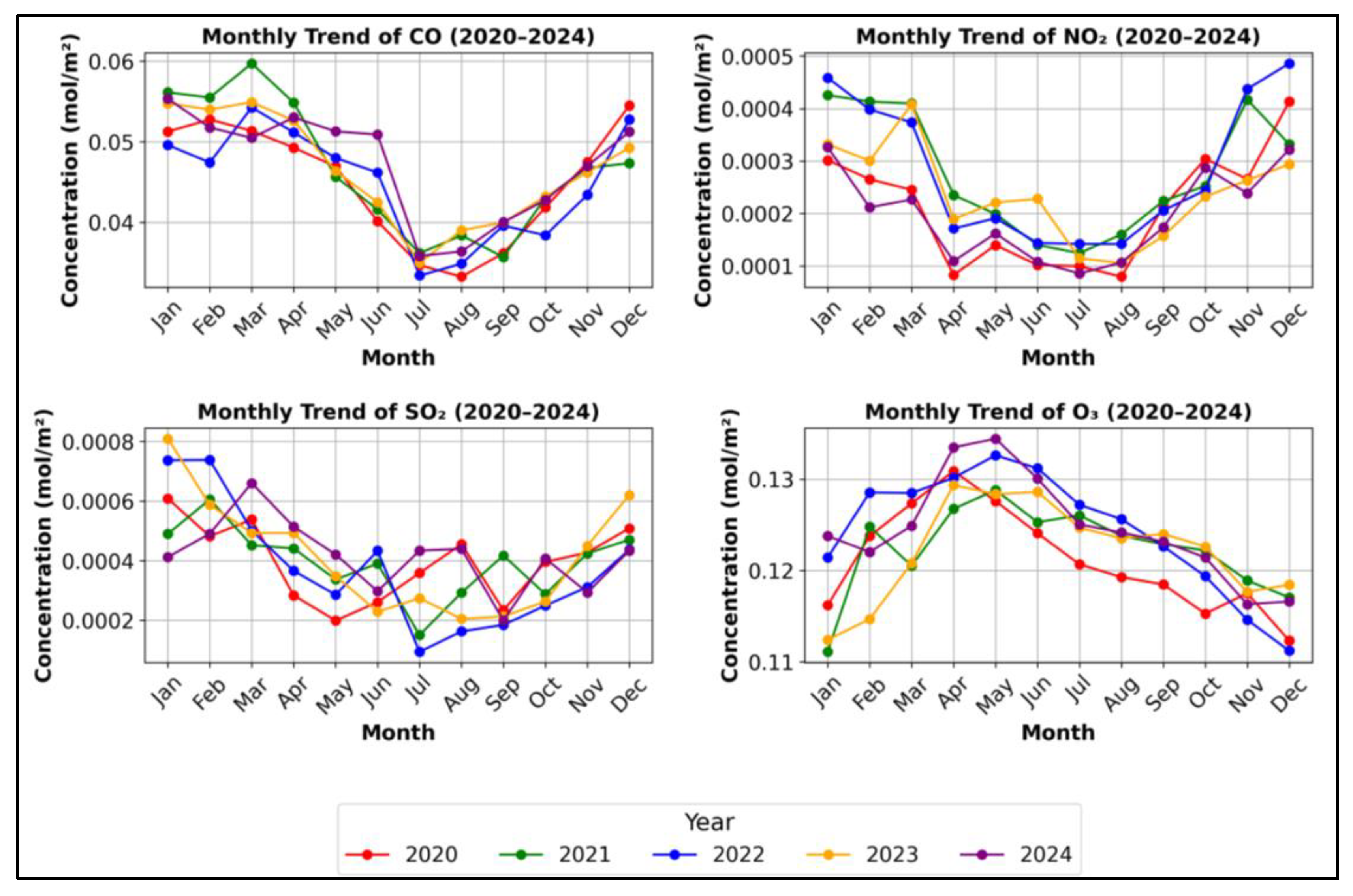
Figure 8.
Man-Kendal test of monthly maximum CO concentration (2020-2024) in Dhaka city.
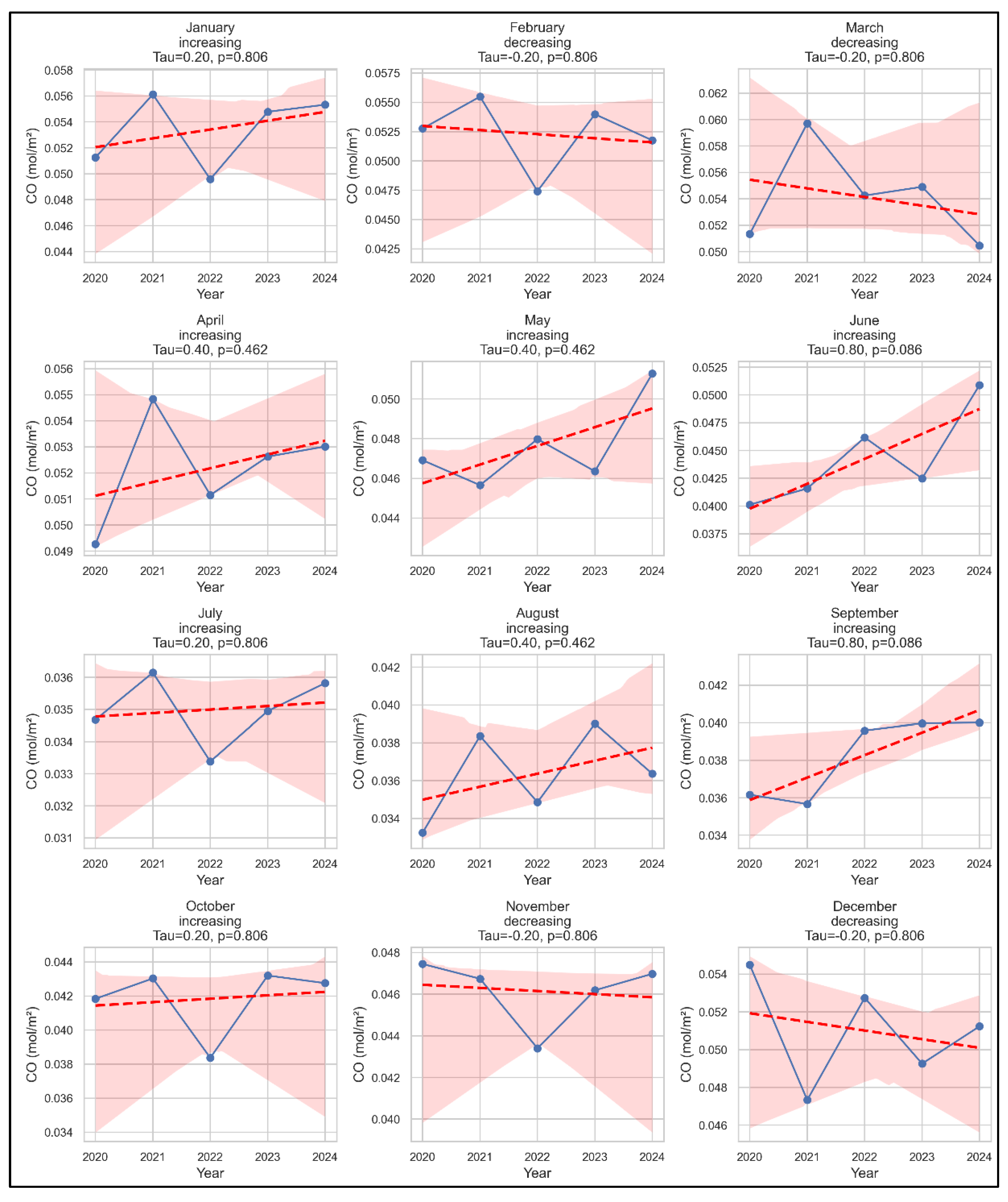
Figure 9.
Man-Kendal test of monthly maximum NO₂ concentration (2020-2024) in Dhaka city.
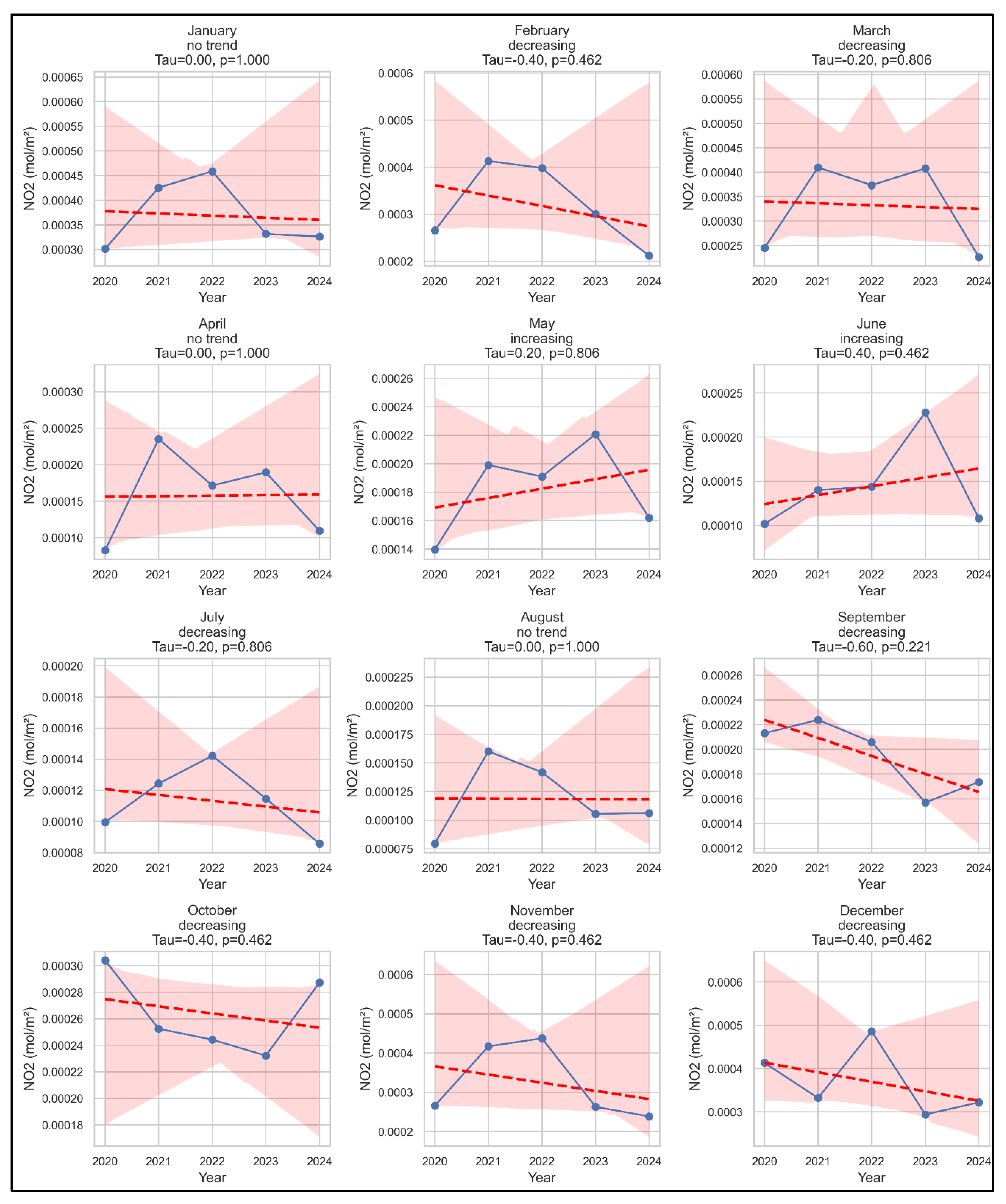
Figure 10.
Man-Kendal test of monthly maximum SO₂ concentration (2020-2024) in Dhaka city.
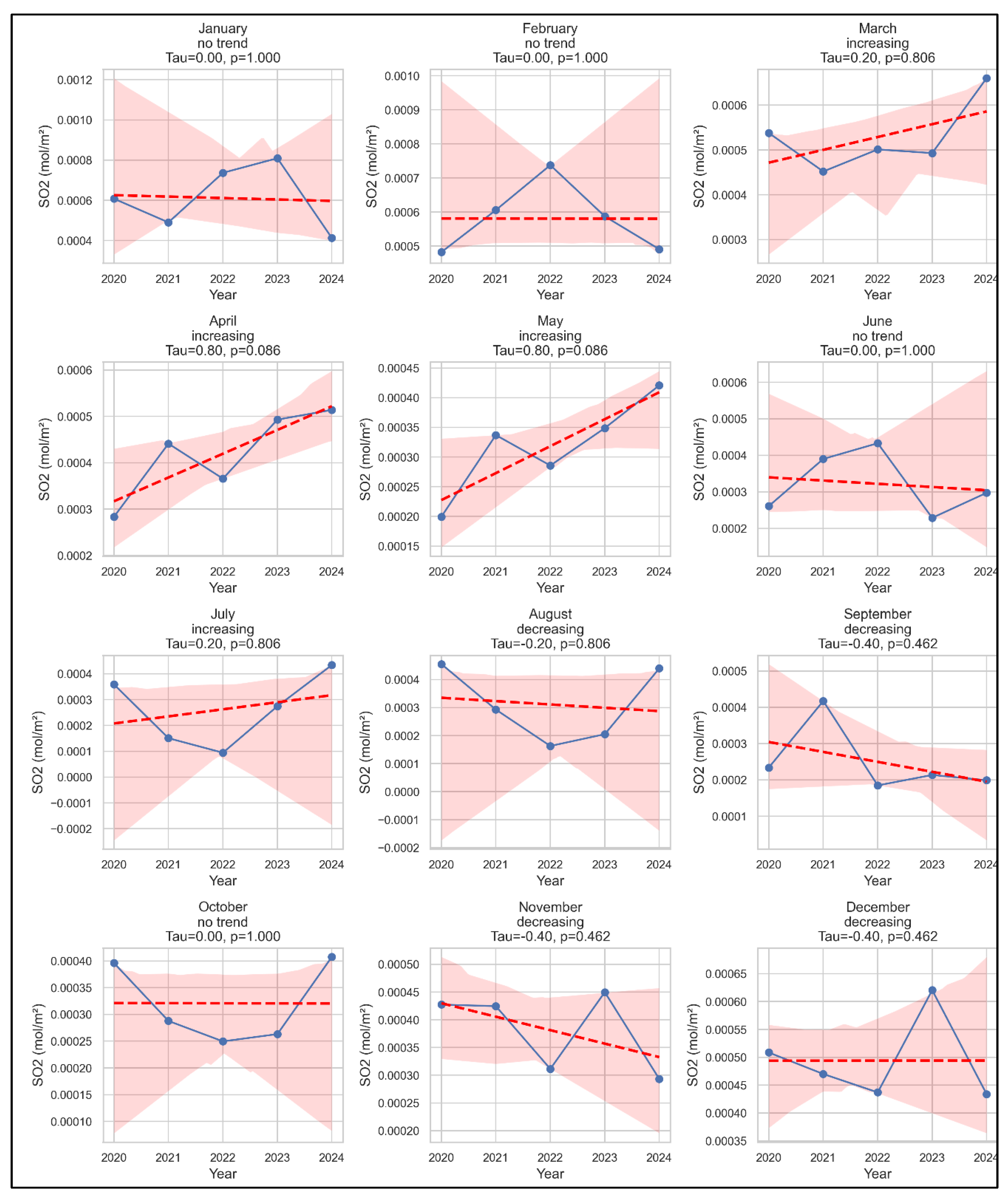
Figure 11.
Man-Kendal test of monthly maximum O3 concentration (2020-2024) in Dhaka city.
Disclaimer/Publisher’s Note: The statements, opinions and data contained in all publications are solely those of the individual author(s) and contributor(s) and not of MDPI and/or the editor(s). MDPI and/or the editor(s) disclaim responsibility for any injury to people or property resulting from any ideas, methods, instructions or products referred to in the content. |
© 2025 by the authors. Licensee MDPI, Basel, Switzerland. This article is an open access article distributed under the terms and conditions of the Creative Commons Attribution (CC BY) license (http://creativecommons.org/licenses/by/4.0/).
Copyright: This open access article is published under a Creative Commons CC BY 4.0 license, which permit the free download, distribution, and reuse, provided that the author and preprint are cited in any reuse.


