
Submitted:
27 March 2025
Posted:
31 March 2025
You are already at the latest version
Abstract
This paper investigates the derivation of global shape functions in T-meshed quadrilateral patches through transfinite interpolation and local elimination. The same shape functions may be alternatively derived starting from a background tensor product of Lagrange polynomials and then imposing linear constraints. Based on the nodal points of the T-mesh, which are associated with the primary degrees of freedom (DOFs), all the other points of the background grid (i.e., the secondary DOFs) are interpolated along horizontal and vertical stations (isolines) of the tensor product, and thus linear relationships are derived. Implementing these constraints into the starting formula in the sense of a Schur complement reduction, the global shape functions associated with the primary degrees of freedom are created. The quality of the elements is verified by the numerical solution of a typical potential problem of second order, with boundary conditions of Dirichlet and Neumann type.
Keywords:
transfinite interpolation
; elimination
; Schur complement reduction
; finite element method.
MSC: 65L60; 65N30; 74S05
1. Introduction
Lagrange polynomials have been extensively used from the very beginning of the Finite Element Method (FEM) [1-3]. First, linear and then quadratic elements were used in conjunction with the isoparametric concept [4]. In the 1980s, a widely accepted assumption was that the complexity in the implementation of elements of higher degree increases considerably, and therefore less attention was devoted to high-order discretization techniques (e.g., Ref. [5], p. 309). However, in the advent of powerful computers, the idea of using polynomials of higher degrees gradually gained acceptance and popularity [6,7]. Two alternative methodologies dealing with high polynomial degrees are: (i) Higher-order Finite Element Method (p-FEM) [8-10] and (ii) Spectral Finite Element Methods (SEM) [11]. The p-method (polynomial order refinement) in FEM increases the degree (p) of the polynomial basis functions used in each element while keeping the mesh fixed. Spectral methods also use high-order polynomial approximations but differ in that they use global basis functions rather than piecewise-defined basis functions. In the paper at hand, we concentrate on a variation of SEM as the topic is elements based on Lagrangian interpolation polynomials.
The opposition in the use of Lagrange polynomials is based on the well-known Runge phenomenon, where a specific non-polynomial function is gradually badly approximated by Lagrange polynomials as far as their degree increases [11-13]. Since the Lagrange polynomials obtain large values near the edges of the interval, it was found that the use of nonuniform node distributions (usually based on Gauß-Lobatto-Chebyshev (GLC) or Gauß-Lobatto-Legendre (GLL) points, which are dense near the ends), lead to excellent results [7,14,15].
Aiming at the easy manipulation and coupling of dissimilar geometric entities, since early 1970s transfinite elements were developed and used in automotive industry [16-18]. In Ref. [18] these elements have been called ‘macroelements’. In the same spirit, within the context of global approximation, which is highly related to SEM, FEM macroelements which occupy the entire or a large portion of the domain have been also successfully used outside the strict context of ideal tensor products of Lagrange polynomials, for example using transfinite interpolation (including Coons interpolation [19]) in conjunction with a few sets of trial functions such as piecewise-linear, B-splines, etc. [20,21]. As it is overviewed in a monograph [22], these elements perform well for the transition between unequally meshed opposite edges of a patch, for the coupling between dissimilar patches, as well as for the treatment of a structured set of internal nodes which do not exactly correspond to the boundary ones [15,23,24]. Among others, typical works in which an entire circle or quadrilateral patch is successfully modeled using a single transfinite element (based on trial functions in the form of Lagrange polynomials) are [25,26].
Unlike structured grids, in 1974, a pilot study demonstrated that it is possible for a rectangular polygon to be decomposed into rectangular cells, where locally blended cubic splines or Hermite interpolation may be applied [27]. Almost forty years later, in 2003, nets of control points which form T-junctions between perpendicular isolines (=const. and =const.), were efficiently treated by Sederberg et al. [28] in the context of computer-aided geometric design (CAGD)-surfaces using B-splines and NURBS and thus were called ‘T-splines’. Since 2010, the application of isogeometric analysis (IGA) using T-splines has been a matter of intensive research to date [29-33].
Based on the above discussion, in the paper at hand, the subdivision of a rectangular domain into non-overlapping quadrilateral elements such that (i) Elements are quadrilaterals (axis-aligned), (ii) T-junctions are allowed (meaning that not all edges need to extend completely across the mesh), and (iii) it is typically hierarchical (allowing local refinements by inserting new elements without disturbing the entire structure), is called ‘T-mesh’.
A recent report has shown that simple T-meshes may be treated using the transfinite interpolation concept, because the auxiliary nodes are automatically eliminated [34]. However, the general T-spline has not been investigated yet. Within this context, the paper at hand investigates the capability of transfinite elements to treat complicated T-meshed patches and eventually proposes a slight extension or an alternative technique using constraints to systematically achieve it. The numerical performance of this approach is verified through a boundary value problem in which the analytical solution of the Laplace equation is of non-polynomial form.
2. Tensor Product Elements
2.1. General Expressions
We consider a reference patch (unit square) in which the horizontal -axis () is uniformly subdivided into segments, and thus the associated Lagrange polynomials (of degree ) form the column vector :
Similarly, the vertical -axis () is uniformly subdivided into segments, and thus the associated Lagrange polynomials (of degree ) form the column vector :
2.2. Quadratic Interpolation
As an example, for a quadratic tensor product element of Lagrange type, the univariate set is defined by the nodes shown in Figure 1a, the element in which is shown in Figure 1b, and thus we have:
and
Substituting Equations (4) to (6) into Equation (3), results in the well-known bi-quadratic shape functions:
3. Traditional Transfinite Elements
There are many higher order macroelements that cannot be described through a tensor product (discussed in Section 2), and some of them have been discussed in Ref. [34]. To prepare the reader for the next section, which is the main topic of the paper at hand, we first focus on traditional structured transfinite elements, which are characterized by some horizontal and vertical stations that are subdivided by several nodes, like those in the 21-node element shown in Figure 2. In Ref. [35], it has been discussed how the individual projectors () of the Boolean sum formulation can be constructed for quadratic blending functions (Lagrange polynomials) and quartic trial functions (Lagrange polynomials. To shorten their presentation, here we prefer an alternative form exploiting matrix notation as follows:
and
According to the standard theory, the transfinite interpolation of bivariate functions expressed be is given by the following Boolean sum:
Substituting the three projectors, i.e., Equations (8) to (10) into Equation (11), extraction of coefficients gives the expression:
where the global bivariate shape functions will be given in terms of univariate Lagrange polynomials by:
As has been previously discussed in [35] and elsewhere, the form of the bivariate shape functions in Equation (13) is generic and can be easily computerized. In brief, nodal points at the intersections of stations (i.e., nodes 1,3,5,9,11,13,17,19,21 in Figure 2) are associated with shape functions () which are influenced by all the three projectors, whereas the rest are influenced by only one projector (the one perpendicular to the isoline the node belongs to). It is worth mentioning that each projector is well-defined by the actual nodes of the mesh and does not require any auxiliary points to be constructed. The set of the 21 shape functions is illustrated in Figure 3.
4. T-Meshed Patch Elements: Constraints and Elimination
In this section, we deal with higher order macroelements that are neither described by a tensor product nor have the form of the traditional structured elements discussed in Section 3. The key characteristic of these elements is that they come from a tensor product in which some nodes are missing. As shown in Figure 4, in general we could categorize these elements in the following three classes:
- Elements where the missing nodes belong to the boundary of the patch (e.g., nodes G and F as illustrated in Figure 4a).
- Elements with hanging internal nodes (denoted by a red cross ) that belong to the extension of isolines in only one direction (e.g., in Figure 4b these isolines are directed toward the -direction).
- Elements with hanging internal nodes that belong to the intersection of two isolines (e.g., node H as illustrated in Figure 4c).
In all formulations of the paper at hand, the missing nodes to form a complete tensor product are initially filled by auxiliary points which are also called ‘artificial’.
Regarding the first category, where the missing nodes belong to the boundary (shown by letter G in Figure 4), obviously they do not influence the interpolation along the corresponding edge, but only influence the interpolation in the vertical direction of the isoline to which they belong. For example, the interpolation along the bottom edges will be of degree and 2 for Figures 4a, 4b, and 4c, respectively, although the artificial node G was introduced. As we shall see below, the bivariate shape functions of these elements associated with boundary nodes on incomplete edges, may be directly obtained applying transfinite interpolation. This happens because each artificial boundary node belongs to the projector having as subscript the direction being vertical to the corresponding edge. For example, nodes G and F (Figure 4a) are involved in the projectors and , respectively, but eventually are automatically eliminated because they appear in the subtracted projector as well.
Concerning the second category, the artificial nodes eventually appear in the projector whose index indicates the direction in which to extend the isoline. This is necessary to connect the internal hanging nodes to the boundary. For example, in Figure 4b we need to extend the two vertical isolines from inside to the bottom edge, and thus the artificial nodes belong to the projector , which is further cancelled by the corresponding terms from the subtracted projector . Note that this is possible, because both projectors are based on the blending functions. Again, with respect to Figure 4b, it should become clear that, if the two nodes that belong to the horizontal isoline 5-6-7-8 had been used to define the trial functions along 5-8 (as a uniform polynomial of six nodes and thus degree 5, instead of as a nonuniform polynomial consisting of nodes 5-6-7-8 and thus of degree 3), then they would have been included in the projector as well, and thus could not be eliminated.
Regarding the third category, the artificial (auxiliary) node H (Figure 4c) belongs to the projector , because it lies at the intersection of the horizontal (4-5) and vertical (8-12-16) stations. For reasons of equal treatment, we cannot prefer a specific direction. Therefore, H will belong to as well as to , resulting in the inability to delete it within the algebraic sum . In general, there are two possible techniques:
- Technique 1: Eliminate H by considering it within the projector but ignoring it within the projector , i.e., considering the trial function along the horizontal isoline to be defined by the nodes (4, 5, and F). However, this trick cannot be applied to complicated T-meshes.
- Technique 2: Interpolate the nodal value at H once along a horizontal and another time along the vertical isoline passing through H and then consider the mean average value of these interpolations. Therefore, it is possible to eliminate the auxiliary node H, as later shown in Subsection 5.5.
5. Constraints
Regarding the first category where the missing nodes belong to the boundary, an indicative collection of elements in which a single boundary node (designated by G) is missing on the bottom edge, is shown in Figure 5. The polynomial interpolation along the bottom edge (to which G belongs) is of degree , and for Figures 5a, 5b, and 5c, respectively. As we will discuss below in Subsections 5.1 to 5.3, the same interpolation is produced when starting from an initial interpolation of one unit higher (, and ) in which the proper constraint is imposed along the nodal points of the bottom edge. The next subsections (5.1 to 5.3) are consistent with the discretization of the bottom edge in the three cases shown in Figure 5. Note that the entire 8-node transfinite element shown in Figure 5a is discussed in detail within Section 5.4.
5.1. Quadratic Polynomials and Linear Constraints
Let us consider a polynomial of second degree, which can be written either in the power form: , or as a sum of three quadratic Lagrange polynomials:
where are the nodal values associated with the nodes (1,2,3) shown in Figure 1a (in local numbering), as well as for the horizontal isolines of Figure 6a, of which the bottom edge is of interest.
If we assume that node 2 is located in the middle of the interval [0,1] (Figure 6a), having the average value of the two ends:
after performing trivial manual operations (replace and with ), we find that the second-order polynomial becomes linear:
In other words, the constraint forces the full quadratic polynomial to degenerate to a linear one.
5.2. Cubic Polynomials and Quadratic Constraints
Now we test the case in which the interpolation is quadratic, however the intermediate (internal) node ‘2’ is not in the middle as usual, but at one-third measured from the left end (i.e., is located at ), and thus the node ‘3’ at position is missing (shown in red color in the right side of Figure 6b). Clearly, we have a unit length with three non-uniform nodes: 1 (at ), 2 (at ), and 4 (at ), and thus non-uniform Lagrange polynomials of degree two are created. In the previously mentioned sequence, node ‘3’ was omitted because it is eliminated from the uniform sequence of four nodes: 1-2-3-4, and thus only the nodes 1-2-4 remain (right part of Figure 6b).
Since node ‘3’ is missing, this in turn means that if we consider the value produced by the non-uniform polynomial of degree 2 at node 3, as a constraint in terms of (), if the latter is introduced into the series expansion of four (cubic) Lagrange polynomials, we shall identically derive the expression of the non-uniform quadratic polynomial.
Actually, considering the three non-uniform Lagrange polynomials (based on the nodal values, ), we obtain:
Setting in Equation (17) the value (), we derive , and thus the constraint becomes:
Using the full cubic Lagrange polynomials based on the uniform interpolation points at (), the univariate function is written in terms of the associated nodal values (, and ) as:
Substituting the constraint described by Equation (18) into the general Equation (19), we receive:
One may observe that the last equality in Equation (20) is identical with the expression of Equation (17). In other words, the imposition of the linear constraint by Equation (18) (which refers to a non-uniform set of Lagrange polynomials of degree ) into the full expression by Equation (19) (which refers to a uniform set of Lagrange polynomials of degree ), results in the same approximation as that of the non-uniform set of Lagrange polynomials.
5.3. Quartic Polynomials and Cubic Constraints
In this section, we consider the nodes with global and local numbering (1-2-3-4-5) along the bottom edge (Figure 6c), where node 2 (at ) is to be eliminated, so as the initial quartic polynomial degenerates to a cubic one (a similar elimination is valid for the bottom edge in Figure 5c).
Since the local node ‘2’ is missing, this in turn means that if we consider the value being produced by the non-uniform cubic polynomial (based on nodes 1-3-4-5) at the point 2, as a constraint in terms of () and the latter is introduced into the series expansion of five (quartic) Lagrange polynomials (based on nodes 1-2-3-4-5), we shall identically derive the expression of the non-uniform cubic polynomial.
Therefore, using the explicit expressions of the four non-uniform Lagrange polynomials of degree (based on the nodal values, ):
when setting the value in Equation (21), we obtain the constraint:
Now we consider the set of uniform Lagrange polynomials of degree , in which the univariate function is approximated as follows:
Substituting the current constraint (i.e., Equation (22)) into Equation (23), results in:
One may observe that the last equality of Equation (24) is identical to Equation (21). In other words, as previously happened, the implementation of the linear constraint forces the full set of uniform Lagrange polynomials of degree ’ to degenerate to the same set as of non-uniform ones with degree .
5.4. Implementation of an Eight-Node Transfinite Element
This subsection discusses the construction of a transfinite element, which is produced by a tensor product with missing boundary nodes. Although the procedure is general, for the sake of brevity we focus on one missing boundary node and a tensor product of quadratic interpolation ().
Therefore, let us consider the 8-node element shown in Figure 7 by adding the inactive auxiliary node G. There are at least two approaches to derive the shape functions of this element, as follows:
5.4.1. Approach 1: Transfinite Interpolation
We construct three projectors, (). To produce , along the middle vertical station at , we need to introduce the artificial (auxiliary) node G (Figure 7), which is everywhere denoted in red color:
In contrast, the artificial node G is not included in the projector , because the representation of along the bottom boundary edge is a-priori linear, and thus we have ():
The third projector is:
One may observe that the artificial node ‘G’ exists in only two out of the three projectors (for which we have ), and thus when the Boolean sum of Equation (11) is implemented, the variable is eventually eliminated. This in turn means that the dependent variable is written in terms of the following eight shape functions:
Regarding the bottom edge 1-2 which is included in the projector , one may observe in the first square brackets of Equation (26) that the univariate function is directly approximated by two polynomials of first degree , and thus no constraint is considered.
5.4.2. Approach 2: Successive Node Elimination from an Initial Tensor Product
In this approach we start with the full tensor product, of which node ‘G’ (Figure 7) is vital part:
Then, in consistency to Section 5.1, we impose the constraint:
Substituting Equation (30) into Equation (29), the action of the basis function , which is the factor of the eliminated variable , is related to two DOFs (i.e., and ), and thus Equation (29) becomes:
Using the explicit form of the quadratic Lagrange polynomials, in :
it can be verified that the two sums involved into Equation (31) simplify to:
Substituting Equation (33) into Equation (31), one may observe that the basis functions, which constitute Approach 2, are identical with those into Equation (28), which constitutes Approach 1. In other words, whether transfinite interpolation is directly applied, or the constraint is implemented into the initial background tensor product, the results are identical.
Interestingly, Equations (28) and (31) show that the shape function associated with each nodal point equals the local tensor product provided linear interpolation along the bottom edge is assumed.
5.5. Elimination of Internal Nodes
In general, the elimination of an internal nodal point is a task that is more difficult than eliminating a boundary node. For example, let us consider the element in Figure 8a in which node 18 (at point H) is to be eliminated. Whatever approach is followed (i.e., transfinite interpolation or background tensor product), the latter point may be considered to belong to the vertical isoline 19-16 as well as to the horizontal isoline 4-20. Obviously, since the value appears in all three projectors () of the transfinite interpolation, it cannot be eliminated by itself in the Boolean sum (Equation (11)) and thus Approach 1 seems to fail as a first single step; therefore, a different treatment is required by extending Approach 1 through a second step. Alternatively, we can deal with Approach 2.
In both approaches, we begin the interpolation through point 18 and seek a straightforward way to eliminate . Since node 18 belongs to the horizontal isoline 4-5-20, it is reasonable to interpolate it along this isoline as a nonuniform quadratic polynomial which comes from the elimination of the third node, like the local nodal value in Equation (18), and thus we have:
On the other hand, node 18 also belongs to the vertical isoline 19-18-8-12-16, and thus plays the role of in Equation (22), whence:
The obvious handling is to take the average of these two constraints, and thus the actual constraint becomes:
It is reminded that Equation (36) is useful for Approach 1 and Approach 2 as well.
6. Construction of the 17-Node and 18-Node T-Mesh Elements
In this section, we will demonstrate the construction of 17-node element (illustrated in Figure 8a) and the 18-node element which would be generated by including node 18 (H) in the formulation.
We recall that having in hand the interpolation of the internal node given by Equation (36), we can follow two alternative but equivalent approaches, i.e., transfinite interpolation or background tensor product formulation. The lowest level of these two approaches were demonstrated in Section 5.4.1 and 5.4.2, respectively.
6.1. Approach 1 to Derive T-Mesh Elements
6.1.1. General Remarks
In Ref. [34], it was shown that in some special cases it is possible to start with the transfinite interpolation formula and eventually lead to a T-spline expression. This is the case when the inserted artificial (auxiliary) nodes, which complete the background (tensor-product) mesh, appear only in two out of the three projectors, and , i.e., either in or in , and thus can be eventually eliminated. For example, if the projector includes all the nodal points of the tensor product background mesh in such a way that (e.g., Figure 4b), then the bivariate variable will be approximated by , which will not include any artificial DOF. Moreover, in the paper at hand, it was made clear that missing nodes at the boundary are easily treated through a simple linear constraint of the nodes along the edge to which the missing node belongs.
Nevertheless, given a quadrilateral patch in which several ordered nodes are interconnected in the form of a T-mesh, we shall see that transfinite interpolation is not always capable of immediately determining the associated shape functions. To make this point clear, below we refer to the 17-node and 18-node elements (Figure 8a) and then in Section 7 we continue with a larger T-mesh.
6.1.2 17- and 18-Node Elements
We consider the T-mesh of seventeen nodal points (1 to 17) shown in Figure 8a, where a rather large gap exists due to three missing points (F, G, H) in the background tensor-product representation (Figure 8b). Nodes 1 to 17 are called primary nodes, whereas the auxiliary points (F, G, H) are called artificial or secondary nodes.
We begin implementing the transfinite interpolation using Lagrange polynomials throughout, and thus all the initial seventeen nodal points, as well as the three artificial ones (F, G, and H created by extension of existing lines), contribute to the formation of the three projectors involved.
Within this patch, the variable of the problem is interpolated by the Boolean sum according to Equation (11). First, we start with the 18-node element and then continue with the 17-node element.
Transfinite Elements Using 18 Nodal Points
Assuming that the blending and trial functions are Lagrange polynomials, the three projectors are given as
and
In more detail, the interpolation along the third vertical station at utilizes the artificial nodes H and G, whereas along the fourth vertical station measured from left (i.e., the edge BC at ) uses only the four primary nodes (3, 9, 13, 17) and thus nonuniform Lagrange polynomials of degree 3 (i.e., the artificial point F(20) is ignored).
Moreover, the interpolation along the bottom horizontal station utilizes the three primary nodes (1, 2, and 3) and nonuniform Lagrange polynomials of degree 2 (i.e., the artificial point G(19) is ignored). Furthermore, regarding the second horizontal station measured from the bottom (at ), the interpolation is performed in terms of the blending functions on the primary (4, 5) continued by the artificial (H, F) nodes.
Also, the tensor product includes all the points involved, i.e., the 17 real nodes and the 3 artificial ones.
Substituting Equations (37) to (39) into the Boolean sum described by Equation (11), one may observe that:
- the two artificial values on the boundary () are eliminated,
- the one in the interior () remains.
Therefore, eighteen shape functions appear in the approximation of the variable
with:
It can be verified that the eighteen global shape functions in Equation (41) fulfil the Partition of Unity Property:
The shape functions of Equation (41) are illustrated in Figure 9b.
One may also observe that all the shape functions of Equation (41) associated with the first seventeen DOFs vanish at the position of point H, i.e., we have . The latter means that a nodal point is necessary to be put at the position of H (called node ‘18’), otherwise the function would vanish at it and the Partition of Unity Property does not hold. In other words, the direct application of the transfinite interpolation to the element of Figure 8a gives the 18-node element.
Transfinite Elements Using 17 Nodal Points
Despite the limitation of transfinite interpolation to automatically derive the shape functions of the 17-node element, Equation (41) concerning the 18-node element (in which the secondary node H(18) exists) may become a useful start for further processing. In more detail, we interpolate using the rest of the nodal values along the horizontal and vertical isolines passing through it, take the mean average and receive again Equation (36). However, the latter is still not applicable because it contains the unknown artificial DOFs and.
Since node 19 is constrained by the node sequence 1-2-3, by virtue of Equation (18), in global numbering we have:
Similarly, since node 20 is constrained by the node sequence 3-9-13-17, by virtue of Equation (22), in global numbering we have:
Substituting Equations (43) and (44) into Equation (36), we eventually receive the following constraint for internal node 18:
One may observe that nodal value is expressed in terms of 11 out of the 17 actual nodal values. Therefore, the substitution of Equation (45) into the expansion of the bivariate function results in:
Equation (46) shows that all the 11 DOFs are affected by (i.e., the shape function of the artificial node H(18), which is described by the lowest equality in Equation (41)). Therefore, after factorization in Equation (46), the set of shape functions of the 17-node element will be given by:
6.2. Approach 2 to Derive the 17-Node and 18-Node T-Mesh Elements
6.2.1. The 18-Node Element
We start with a background tensor product mesh element, of size 4 × 5 (i.e., 20-node element), shown in Figure 8b, in which the bivariate function is approximated by:
where is the -th nodal value whereas denotes the same in terms of the associated univariate Lagrange polynomials. It is noted that the set of Lagrange polynomials , which are involved in Equation (48), coincides with the set of blending functions , whereas the set of Lagrange polynomials coincides with the set of blending functions , by definition. Thus, we can write and , which means that the symbols and can be used interchangeably.
Regarding the 18-node element, it may be produced from the tensor product mesh, in which the two boundary nodes (G, F) are secondary (not independent) and thus must be eliminated. These nodes simply lie inside the intervals made by the nonuniform nodes 1-2-3 (at ) and 3-9-13-17 (at ), respectively. Therefore, based on these nonuniform Lagrange polynomials, and applying Equations (18) and (22), we can put the following constraints on the points G and F along the edges AB and BC, respectively:
and
Substituting Equations (49) and (50) into Equation (48), and then extracting the common factors, we receive:
One may observe in Equation (51) that six out of the total eighteen DOFs, i.e. the nodal values (located along the edges AB and BC), are not associated with a simple tensor product of the blending functions. This fact may be also observed in Equation (41), in which the associated shape functions include the non-uniform Lagrange polynomials (along the edge AB) and (along the edge BC).
Of course, it is trivial to prove that each of the above non-tensor product shape functions are identical (i.e., ), in both Equation (41) and Equation (51). For example, the modified shape function of the nodal point ‘1’ is written as:
and, eventually, becomes identical to the nonuniform Lagrange polynomial involved in the first equality of Equation (41).
6.2.2. The 17-Node Element
Substituting Equation (45) into Equation (51), we obtain:
One may observe that all the seventeen shape functions in Equation (53) have been expressed in terms of the blending functions only, and thus the accurate representation of the boundary conditions is not obvious yet. Nevertheless, it can be easily verified that the shape functions of Equation (53), which are associated with boundary nodes, give the same result as that produced by the nonuniform Lagrange polynomials in each edge. For example, the shape function , which is associated with the corner node A(1) of Figure 8a, was drawn along the mutually vertical edges AD and AB (shown in Figure 8b), and was found to coincide with the polynomials (determined by the uniform node sequence {0,1/4,2/4,3/4,1} and the nonuniform one {0,1/3,1}, respectively). Alternatively, by substituting the analytical expressions of the equal-spaced univariate Lagrange polynomials and in the first equality of Equation (53), the reader may prove the same thing.
Moreover, despite their slightly different analytical forms, one may easily show (theoretically and numerically) that each of the 17 equalities in Equation (53) is identical to the corresponding equality in Equation (47).
In conclusion, the desired 17-node element can be derived either using Approach 1 (transfinite interpolation) accompanied by the imposition of a constraint for only the internal node H(18) or following Approach 2 (background tensor product) in which the constraint for internal node 18 is followed by the constraints at the boundary nodes G(19) and F(20).
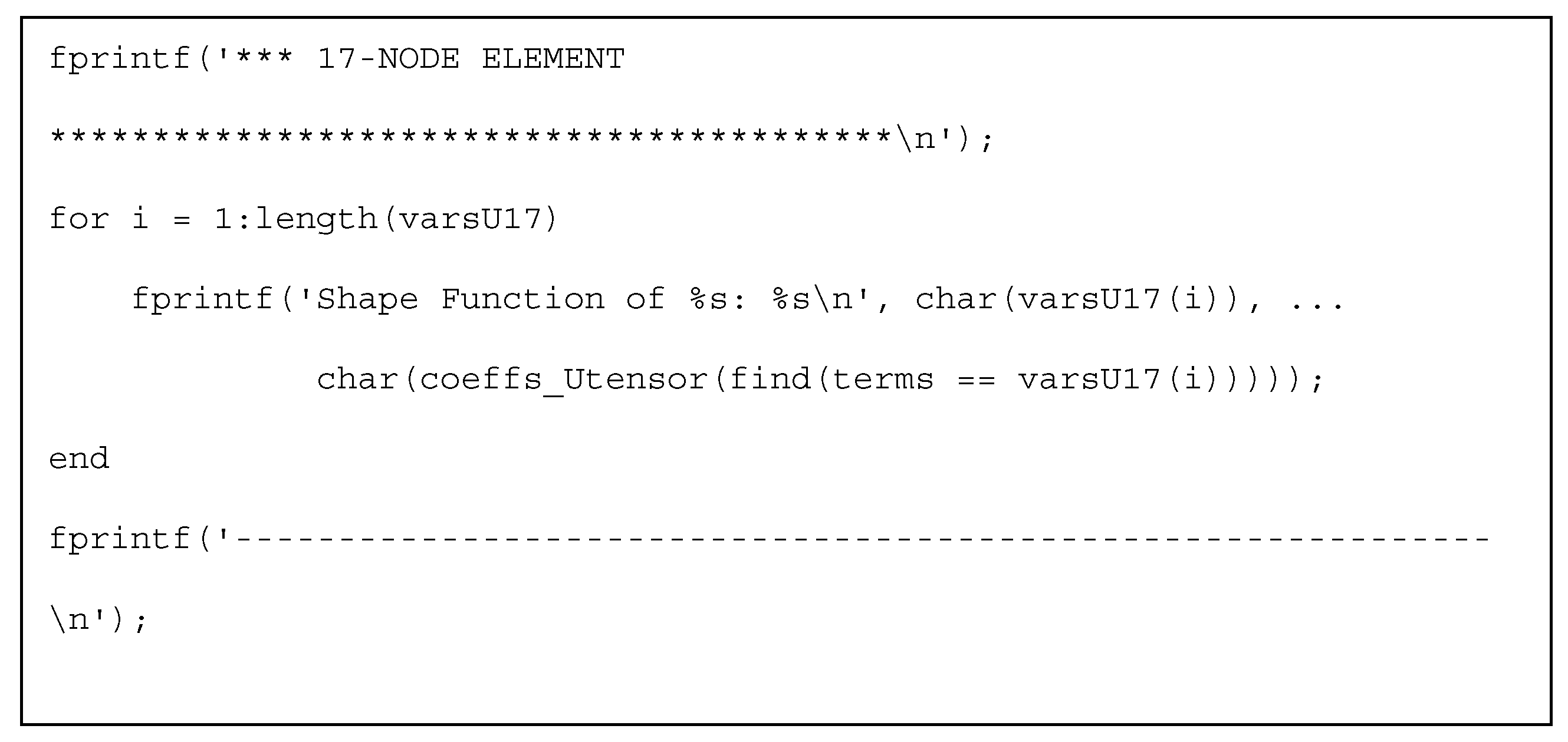
A MATLAB® code which deals with all the three T-mesh elements (19-, 18-, and 17-node), including the background tensor product, is cited in Appendix A.
7. 46-Node T-Element
7.1. Description of the Stations
Let us consider the index space of the T-mesh shown in Figure 10 (with parameters ), which is inspired by Ref. [29](p. 244), but was purposely extended for a Lagrange based formulation adding one extra layer along the entire boundary.
One reason for the above choice is that it is clearly written in Ref. [29](p. 243) that this index space does not ensure a-priori the Partition of Unit Property (PUP), whereas another reason is its complexity and thus its treatment is instructive for judgement of the previously presented methodology in practical applications.
One may observe that the nodes, numbered from 1 to 46, belong to 9 horizontal and 9 vertical stations, which overall determine a uniform background mesh (tensor product required to form the projector ) of 9 × 9 = 81 points in total. Again, all the 81 background nodes need to be considered in the beginning, because all of them contribute to the projector . Therefore, since only 46 out of the 81 total points are primary nodes associated with 46 degrees of freedom, there will be secondary nodes as well. Moreover, since 11 out of the 35 secondary nodes belong to the boundary, there will be only 24 secondary nodes in the interior of the element. This in turn means that if Approach 1 is adopted (i.e., transfinite interpolation), we need only 24 constraints, one for each internal secondary node. Alternatively, if Approach 2 is adopted (background tensor product), we need 35 constraints, because the secondary boundary nodes will be equally treated.
In this specific T-element, the complexity is high, because among the total 18 stations only one of them is uniformly meshed (i.e., the third vertical one, measured from left) whereas in all the other 17 stations at least one out of the local 9 background nodes is missing.
In a tensor product with missing nodes, all empty node positions must first be filled in. Regarding the boundary, the artificial nodes (51,61) on bottom edge AB belong to only two projectors, i.e. (non-uniform polynomials with respect to parameter along isolines 51-43 and 61-44, respectively) and . Nevertheless, the associated shape functions and are not eliminated, because consists of uniform blending functions whereas consists of non-uniform polynomials (elimination restricts to the boundary only). Similarly, the artificial nodes of BC (72,75,78) belong to (non-uniform polynomial with respect to parameter along isolines 69-72, 28-75, and 79-78, respectively) and are not eliminated as well (as previously, elimination restricts to the boundary only). For each completed node, it is a matter of choosing in which isoline direction it will be considered. Here, a question arises:
Is it possible to number the auxiliary secondary nodes in a clever way so as they appear only twice in the Boolean sum?
For example, secondary nodes 47-64-48-49-50 may be chosen to belong to the vertical isoline , where they create a uniform partition of it, and thus this part of the projector is cancelled by the corresponding part of the projector . On the other hand, the secondary nodes 52-to-54 present the following difficulty. To have uniformity along the isoline , node 81 would have to be included. However, node 81 is also necessary (along with 64) for the formation of along the uniformly partitioned isoline .
From the above discussion it becomes clear that for a general T-meshed patch (T-element) like that of Figure 10, it is not possible to find a sequence of nodal points along all the isolines, which will ensure that secondary nodes belong to only two out of the three projectors. Therefore, no tricks will be adopted, and each station will be described mainly by its corresponding primary nodes. Below, the terms secondary, auxiliary, or artificial, will be equally used.
Let us again consider interpolation using Lagrange polynomials for the entire element. Then, the blending functions of the transfinite interpolation will be uniform Lagrange polynomials of degree 8, in either of the two directions and . Regarding the formation of the three projectors, each station must be taken with its individual set of trial functions (based on the primary nodes and the secondary nodes, when there is no support). To facilitate understanding the procedure, the horizontal isolines and the associated auxiliary (secondary) points have been drawn in blue color, whereas the vertical ones in red color. In addition, auxiliary points at intersection have been drawn in green color.
In more detail, regarding the horizontal stations we have the following trial functions
- Station H1 at , which is defined by the seven nodes , is described by a set of 7 nonuniform Lagrange polynomials. All the involved nodes are primary.
- Station H2 at , which is defined by the seven nodes (), is again described by a set of 7 nonuniform Lagrange polynomials. All the involved nodes are primary.
- Station H3 at , which is defined by the seven nodes , is described by a set of 7 nonuniform Lagrange polynomials. Note that the first two nodes are secondary and are required to complete the support on the left part of station H3, whereas the auxiliary (background) nodes 53 and 63 are not required because they are between existing supports.
- Station H4 at , which is defined by the seven nodes, is described by a set of 7 nonuniform Lagrange polynomials. Note that the first two nodes are secondary.
- Station H5 at , which is defined by the seven nodes , is described by a set of 7 nonuniform Lagrange polynomials. Note that here, in addition to the first secondary nodes , additional auxiliary nodes are used to complete the support on the right side of the station.
- Station H6 at , which is defined by the seven nodes of which the last four are secondary, is described by a set of 7 nonuniform Lagrange polynomials.
- Station H7 at , which is defined by the nodes , of which five are secondary, is described by a set of 7 nonuniform Lagrange polynomials.
- Station H8 at , which is defined by the nodes , is described by a set of 7 nonuniform Lagrange polynomials. All the involved nodes are primary.
- Station H9 at , which is defined by the seven nodes , is described by a set of 7 nonuniform Lagrange polynomials. All the involved nodes are primary.
- One may observe that all the above trial functions are nonuniform polynomials of the same degree 7, but this is an accidental event (which does not occur for the vertical stations).
- Regarding the vertical stations we have the following trial functions
- Station V1 at , which is defined by the five nodes , is described by a set of 5 nonuniform Lagrange polynomials. All the involved nodes are primary.
- Station V2 at , which is defined by the five nodes , is described by a set of 5 nonuniform Lagrange polynomials. All the involved nodes are primary.
- Station V3 at , which is defined by the nine nodes , is described by a set of 9 uniform Lagrange polynomials. All the involved nodes are primary, and it is the only station which involves the maximum allowable number of nine primary nodes.
- Station V4 at , which is defined by the eight nodes of which the last four are secondary, is described by a set of 8 nonuniform Lagrange polynomials.
- Station V5 at , which is defined by the eight nodes of which the first four are secondary, is described by a set of 8 nonuniform Lagrange polynomials.
- Station V6 at , which is defined by the seven nodes of which the last four are secondary, is described by a set of 7 nonuniform Lagrange polynomials. Note the big gap between the secondary nodes and .
- Station V7 at , which is defined by the seven nodes of which the first three are secondary, is described by a set of 7 nonuniform Lagrange polynomials. Note the big gap between and .
- Station V8 at , which is defined by the six nodes , is described by a set of 6 nonuniform Lagrange polynomials. Note that all the involved nodes are primary, while there is a big gap between and .
- Station V9 at , which is defined by the six nodes , is described by a set of 6 nonuniform Lagrange polynomials. Note that all the involved nodes are primary, while there is a big gap between and .
Based on the above blending and trial functions, the Boolean sum of Equation (11) was found to include shape functions associated with all the primary nodes 1 to 46 as well as all the artificial nodes (81 nonzero shape functions in total). In other words, for the T-mesh shown in Figure 10, transfinite interpolation is not capable by itself of producing a set of 46 global shape functions possessing the Partition of Unity Property. Therefore, a different approach is required to resolve this problem.
7.2. Imposition of Linear Constraints at Secondary Nodes
As was discussed earlier, we may follow either Approach 1 or Approach 2.
7.2.1. Approach 1:
We apply transfinite interpolation, initially considering all the 81 nodes (primary and secondary). The 11 secondary nodes on the boundary do not contribute because the boundary is interpolated through the primary nodal values only, whereas each secondary node on the boundary is involved in only two projectors and thus are eventually eliminated. Therefore, in this approach we deal with only the remaining 24 secondary nodes in the interior, of which 21 belong to isolines and thus are easily eliminated applying simple linear constraints like those of Equations (15), (18) and (22). Regarding the secondary internal nodes 57, 58 and 64, we apply the mean average procedure. Thus, overall, we must deal with a total of 24 linear constraints in the general form:
where is the column vector (of size 35 × 1) which includes the secondary DOFs, is the column vector (of size 46 × 1) which includes the primary DOFs, and is the transformation matrix (of size 35 × 46) which relates the secondary DOFs in terms of the primary ones. When Equation (54) is considered, the tensor products associated with the secondary DOFs are embodied into the primary DOFs , and thus a set of 46 bivariate shape functions is eventually produced.
7.2.2. Approach 2
We blindly start with the complete tensor product of the 81 nodes in a background mesh, without being interested whether a node lies on the boundary or not:
In this initial state, if the nodal value is associated with the intersection of the row and column in the T-mesh, the global shape function is given by the tensor product as
As we discussed in the previous section, the univariate trial function at each station was determined in terms of the primary DOFs (). The next step is to interpolate the auxiliary DOFs ( to ) in terms of the primary DOFs ( to ). To this purpose we distinguish two cases:
- If the auxiliary DOF clearly belongs to a single station ( or ), then we interpolate in terms of the nodal values associated with this specific station. All the auxiliary nodes except of three ones belong to this category (see below).
- If the auxiliary DOF does not clearly belong to a single station but to the intersection of two sections, then we interpolate , in both directions, using the mean average of the two values (one for the horizontal and the other for the vertical section). For the configuration of Figure 10, the relevant nodes (for averaging like Equation (36)) are 57, 58 and 64.
- Therefore, for the 46node T-element of this section, we impose 32 simple interpolations along either horizontal or vertical isolines and 3 averaging procedures using both mutually perpendicular isolines passing through the intersected nodes (57, 58 and 64).
Practically, we create a function which calculates the values of all the Lagrange polynomials associated with any given node sequence. Using this function, we identify the section to which a secondary point belongs, and thus we calculate the 35 nodal values in terms of the primary ones () and may be in terms of some secondary values as well. Using symbol manipulation software, we express the secondary DOFs in terms of the primary ones, and in this way (elimination process) we eventually determine closed-form analytical expressions for all the global shape functions, .
- For example, considering the nonuniform Lagrange polynomials based on the nodal points (1,2,3,4,5,6,7) on the bottom edge AB of the quadrilateral patch, the nodal values at the points 51 and 61 are eliminated in terms of the primary nodal values of the same edge by the linear relationships:
- Similar constraints such as those of Equation (57) are obtained for the 17 (i.e., not all the 18) iso-lines and for all the secondary nodes except for (57, 58, and 64) which belong to two isolines simultaneously. As already mentioned, for the latter three secondary nodes, we take the mean average of the two constraints as previously shown in Equation (36).
- Since the secondary nodes are a linear combination of the primary ones (a portion given by Equation (57)), we can eventually find a numerical matrix (of size 35 × 46), according to Equation (54). Obviously, when Equation (54) is considered in the tensor product of the 81 terms, this will be eventually expressed in terms of the 46 primary variables only (i.e., the vector ). The procedure is very similar to that for a smaller mesh (see Subsection 6.2.2), which was described in detail through a MATLAB® computer program in Appendix A.
Implementing the above approach, the 46 shape functions are illustrated in Figure 11. It was validated that they fulfil the Partition of Unity Property. The analytical expressions are given in Appendix B.
8. Numerical Verification
In addition to the above theoretical presentation regarding the construction of the shape functions in T-elements, below we demonstrate the numerical performance of the above elements in the following boundary value problem (BVP) that is characterized by different polynomial degrees in each direction and a non-polynomial exact solution.
Example : Heat-flow in rectangular sheet
Let us consider a square sheet of dimensions () in which a Laplace equation governs physics. The boundary conditions are partially Dirichlet and Neumann type, as shown in Figure 12a. The temperature along the top edge is given as
The exact solution is given as:
whereas the error norm , is defined as:
Solution: The entire patch ABCD was discretized as a single tensor product element of 20 degrees of freedom (DOF) shown in Figure 12b (with polynomial degrees and ), of which only nine DOF are unrestrained. Using Lagrange polynomials, the error norm was found to be .
It is worth mentioning that next to the above tensor product, we further used non-uniform Lagrange polynomials toward the y-direction, with nodal points at (i.e., slightly refined close to the top edge DC). It was found that, in the formulation using nonuniform Lagrange polynomials, the L2-norm was practically insensitive, since it changed with respect to the above uniform solution only after the 13th decimal point. Despite the non-uniform location of nodal points in the y-direction, the linear mapping was preserved (i.e., and ) and (closely related) the determinant of the Jacobian was always constant, equal to unity.
For all the elements developed in the paper at hand, which model the entire unit square patch as a single macroelement, the calculated L2 error norm is shown in Table 1. One may observe that:
- The accuracy of the 8-node transfinite element is acceptable.
- The accuracy of the traditional 21-node transfinite element is excellent.
- The accuracy in the 17-, 18-, and 20-node transfinite elements is acceptable and very similar.
- The additional constraints to come from a 20 to an 18 and 17 node element decrease the accuracy
- The constraints on internal secondary nodes are worse for the accuracy.
- The accuracy of the complicated 46-node T-element is the best of all.
9. Discussion
In computational mechanics, one disadvantage of the tensor product is that it requires the same number and the same relative location of nodes on opposite edges of a large element or patch. Therefore, these nodes must be arranged along discrete isolines. This in turn leads to connectivity problems when two dissimilar patches must be joined together. As a result, the construction of special ‘transition’ elements is imperative. Such elements can be automatically generated using the transfinite interpolation.
Moreover, the existence of high gradients requires local mesh refinement leading to ‘hanging nodes’, but this issue is easily treated through the transfinite interpolation, using a larger number of stations close to the singularity. The hanging nodes are treated by implicitly extending the isolines to which they belong until they reach the boundary. However, the produced nodes are ‘artificial’, in the sense that they are not eventually involved in the final expressions. This happened in all test cases investigated by the authors so far (before the paper at hand), just because the isolines were in no case intersected.
Beyond the above state-of-the-art, in cases where some isolines are intersected at points where no primary node exists, the present paper proposes the substitution of this nodal value at the intersection (associated with a secondary DOF) through a linear constraint which is based on the primary nodal points along these two isolines. Although this procedure would be sufficient and complete this research, the paper continues and shows that, in principle, it would be also possible to start with a background tensor product and then impose linear constraints between secondary and primary DOFs along the boundary and the interior. In this way, since secondary DOFs are related with the primary DOFs through a (generally non-square) matrix (i.e., ), it is a trivial task to reshape the initial tensor product into a set of global shape functions associated with only the primary DOFs . For 17-, 18-, and 19-node elements, the procedure was fully explained in Appendix A.
10. Conclusions
It was shown that in T-elements with mutual vertical isolines which may be intersected at points where no primary node exists, the transfinite interpolation may not directly eliminate the nodal values of primary degrees of freedom. A remedy was proposed, and it consists of the elimination of the secondary degrees of freedom at the intersection of these isolines using the primary nodal values lying along these isolines. Alternatively, it was shown that an equivalent approach is to begin with a tensor product and then successively impose the linear constraints which constitute the elimination of the secondary in terms of the primary degrees of freedom.
Supplementary Materials
The following supporting information can be downloaded at the website of this paper posted on Preprints.org.
Author Contributions
“Conceptualization, C.P. and S.E.; methodology, C.P. and S.E.; software, C.P.; validation, S.E.; writing—original draft preparation, C.P.; writing—review and editing, S.E..; visualization, S.E.; supervision, C.P.; project administration, C.P. All authors have read and agreed to the published version of the manuscript.” Please turn to the CRediT taxonomy for the term explanation. Authorship must be limited to those who have contributed substantially to the work reported.
Funding
This research received no external funding.
Conflicts of Interest
The authors declare no conflicts of interest.
Appendix A: Shape functions of 17-, 18-, and 19-node T-Mesh Elements
For a given nodal squence x_nodes, and a given value x_v, the associated Lagrange polynomials can be calculated using the following MATLAB function:
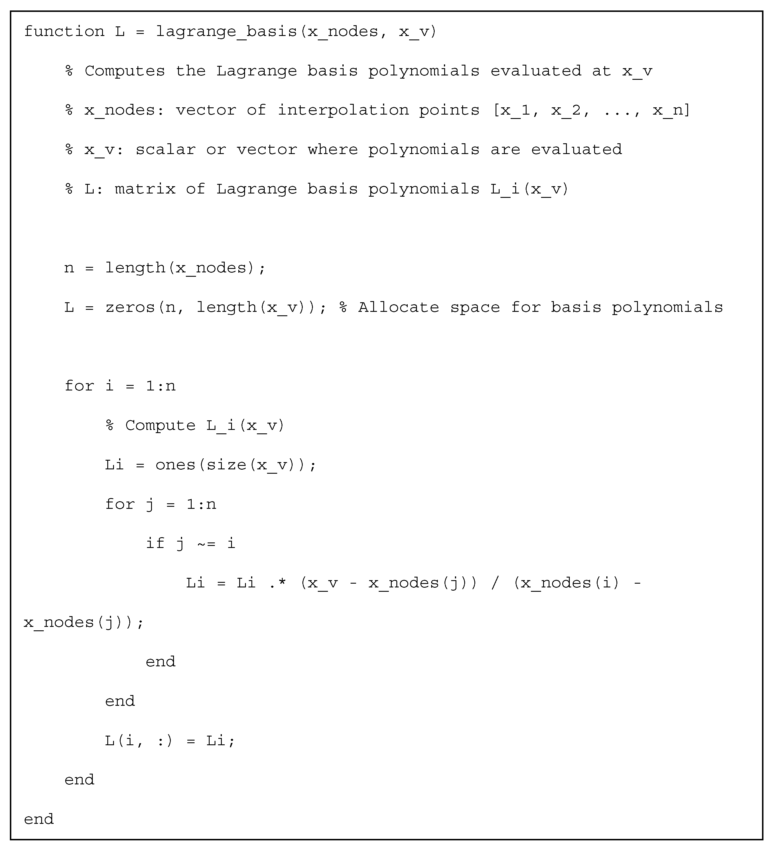
For example, considering the bottom edge of the 17-node element shown in Figure 8a, we have x_nodes=[0,1/3,1]. Applying the above function lagrange_basis at x_v=2/3:
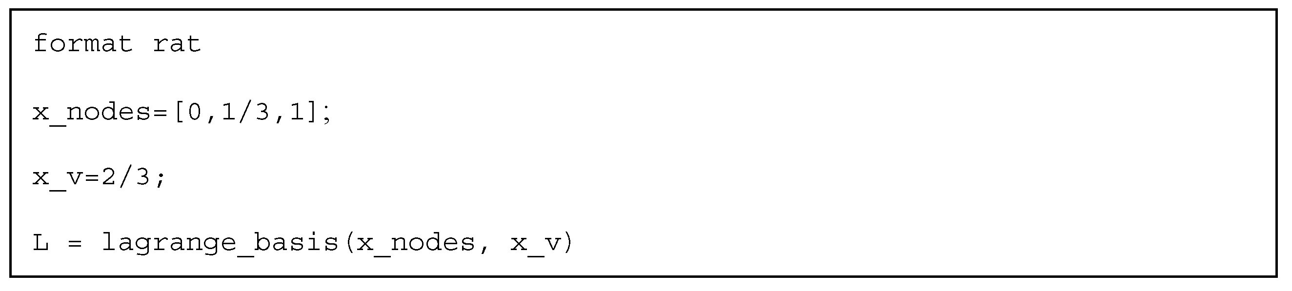
the runout of the above computer program is:
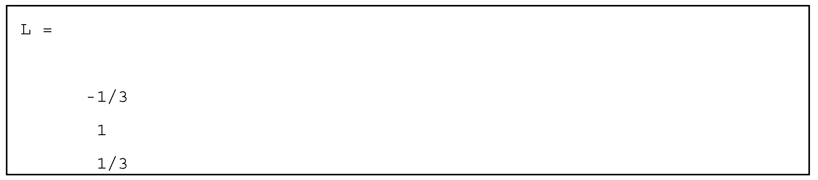
in which one may recognize the three coefficients involved in Equation (18), which also refers to node G(19) on the bottom edge of the T-element shown in Figure 8a.
Regarding the same set of T-mesh elements (shown in Figure 8a), below we present a MATLAB® code (PROGRAM-1), which incorporates ready-made constraints (as those determined above), then it finds the analytical form of the shape functions of the T-element, and eventually displays them:
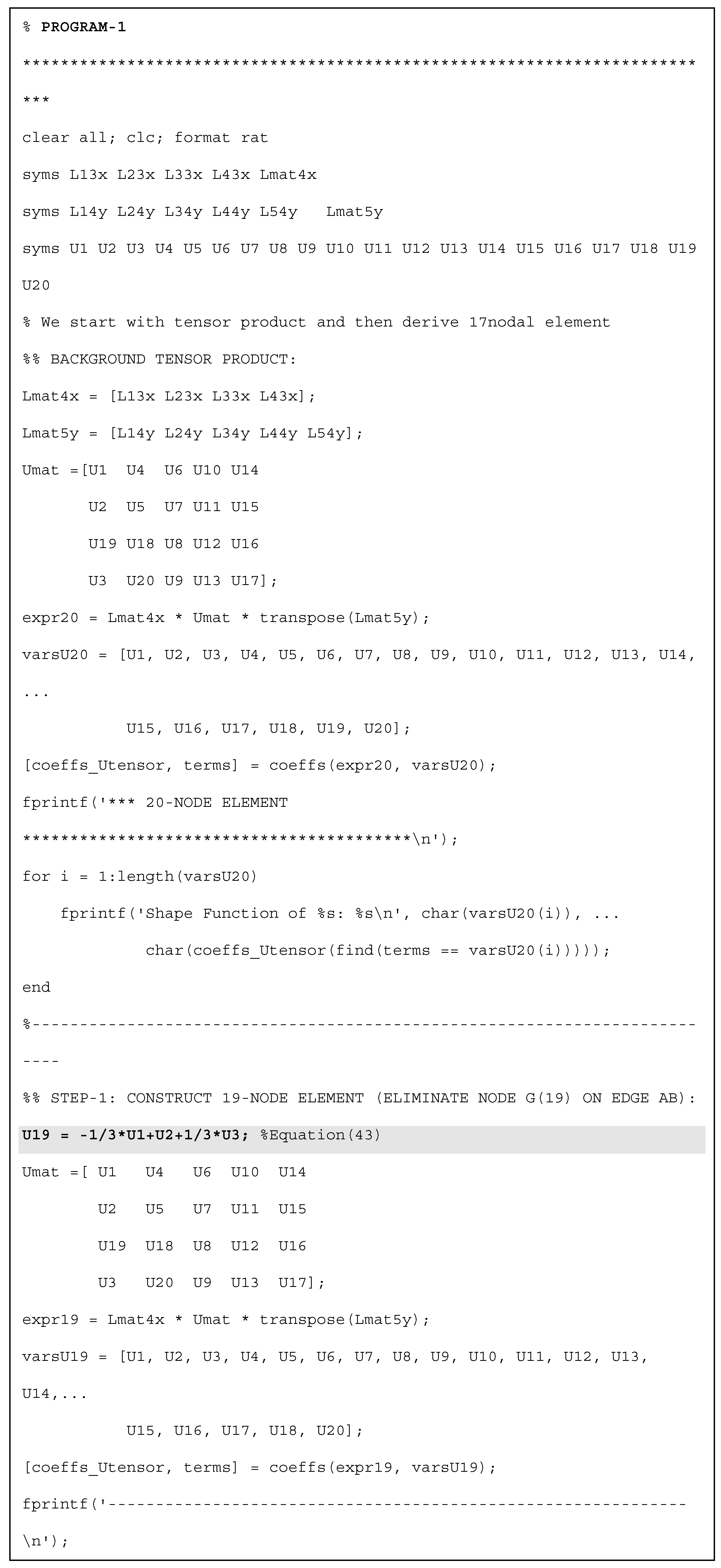
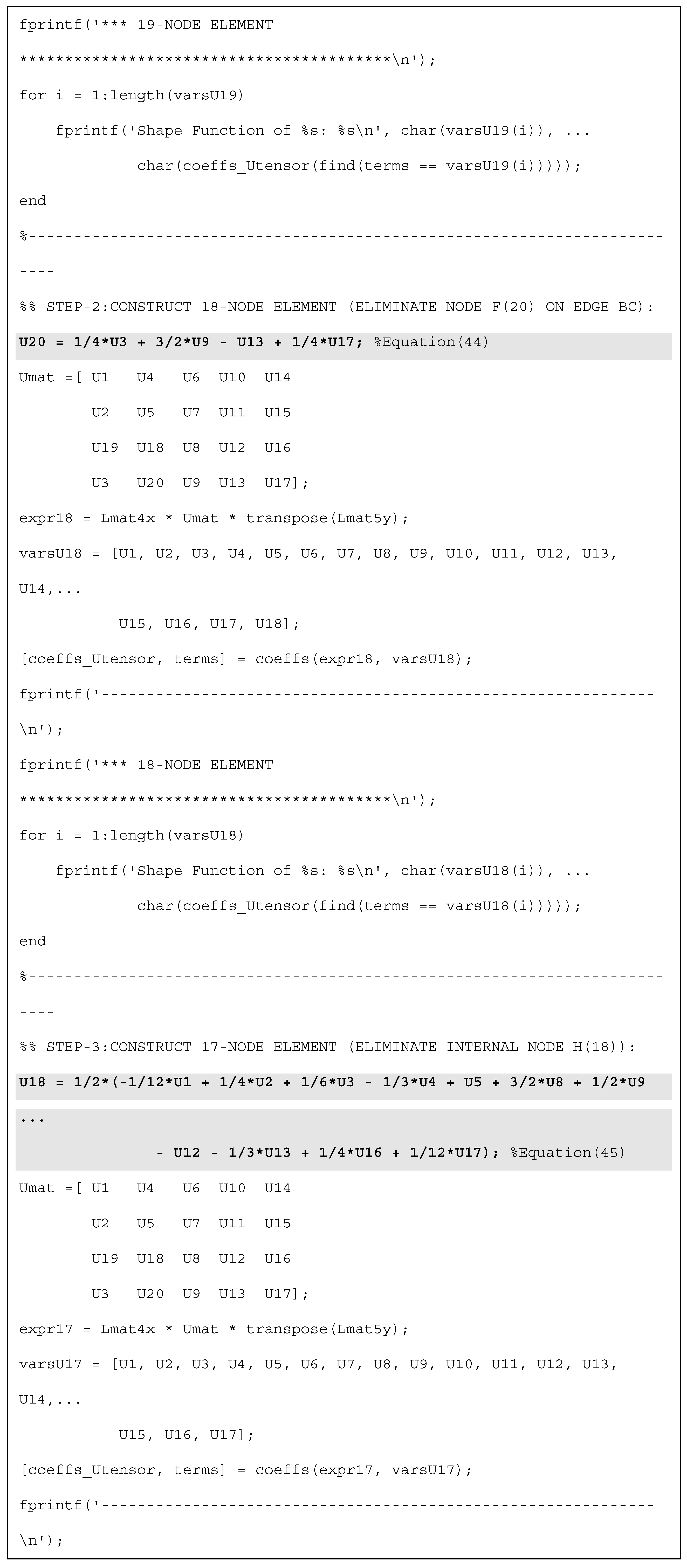
One may observe in PROGRAM-1 that triplet , which was determined in the beginning of Appendix A (and refers to Equation (43)), has been incorporated in the shadowed line #25. Similarly, the coefficients involved in Equations (44) and (45) have been incorporated in the shadowed lines #42, and #59 of PROGRAM-1.
Moreover, regarding the 17-node element, if one combines the three constraints given by Equations (43) to (45), and cited in the three shadowed lines of PROGRAM-1 as well, he/she will find that the transformation matrix S, which relates the secondary with the primary DOFs in the general form of Equation (54), will be given as follows:
Appendix B: Global Shape Functions of the 46node T-like Element
Using uniform Lagrange polynomials of degree
for implementing the blending functions
and , the bivariate global shape functions of the 46-node element which is shown in Figure 10, are given by the following lengthy expression:
References
- Zienkiewicz, O.C.; Taylor, R.L.; Zhu, J.Z. The Finite Element Method, 7th ed. Butterworth-Heinemann, Oxford, 2013.
- Bathe, K.-J. Finite Element Procedures, 2nd edition ed. Bathe, K.-J., Watertown, MA, 2014.
- Hughes, T.J.R. The Finite Element Method. Dover Publications, Mineola, NY, 2000.
- Taig, I.C. Structural analysis by the matrix displacement method. Tech. rep., British Aircraft Corporation, Warton Aerodrome: English Electric Aviation Limited, Report Number SO 17 based on work performed ca. 1957, 1962.
- Brebbia, C.A.; Ferrante, A.J. Computational Methods for the Solution of Engineering Problems, 3rd rev ed. Pentech Pr., London, 1986.
- Szabó, B.; Babuška, I. Finite Element Analysis. Wiley, New York, 1991.
- Rønquist, E.M.; Patera, A.T. A Legendre spectral element method for the Stefan problem. International Journal for Numerical Methods in Engineering 1987, 24, 2273–2299. [Google Scholar] [CrossRef]
- I. Babuska, B. A. Szabo, and I. N. Katz. The p-Version of the Finite Element Method. SIAM Journal on Numerical Analysis 1981, 18, 515–545. [CrossRef]
- Szabó, B.; Düster, A.; Rank, E. The p-Version of the Finite Element Method. In: Encyclopedia of Computational Mechanics (eds E. Stein, R. Borst and T.J.R. Hughes), 2004. [CrossRef]
- El-Zafrany, A.; Cookson, R.A. Derivation of Lagrangian and Hermitian shape functions for quadrilateral elements. International Journal for Numerical Methods in Engineering 1986, 23(10), 1939–1958. [Google Scholar] [CrossRef]
- Pozrikidis, C. Introduction to Finite and Spectral Element Methods Using MATLAB, 2nd ed. CRC Press, New Yrk, 2014. [CrossRef]
- de Boor, C. A Practical Guide to Splines, rev ed. Springer, New York, 2001.
- Eisenträger, S.; Kapuria, S.; Jain, M.; Zhang, J. On the Numerical Properties of High-Order Spectral (Euler-Bernoulli) Beam Elements, Z Angew Math Mech. 2023, 103(9), e202200422 (2023). [CrossRef]
- Patera, A.T. A spectral element method for fluid dynamics: Laminar flow in a channel expansion. Journal of Computational Physics 1984, 54(3), 468–488. [Google Scholar] [CrossRef]
- Eisenträger, S.; Eisenträger, J.; Gravenkamp, H.; Provatidis, C.G. High order transition elements: The xNy-element concept, Part II: Dynamics. Comput. Methods Appl. Mech. Eng. 2021, 387, 114145. [Google Scholar] [CrossRef]
- Gordon, W.J.; Hall, C.A. Transfinite element methods: Blending-function interpolation over arbitrary curved element domains. Numerische Mathematik 1973, 21, 109–129. [Google Scholar] [CrossRef]
- Cavendish, J.C.; Gordon, W.J.; Hall, C.A. Ritz-Galerkin approximations in blending function spaces. Numerische Mathematik 1976, 26, 155–178. [Google Scholar] [CrossRef]
- Cavendish, J.C.; Gordon, W.J.; Hall, C.A. Substructured macro elements based on locally blended interpolation. International Journal for Numerical Methods in Engineering 1977, 11, 1405–1421. [Google Scholar] [CrossRef]
- Coons, S.A. Surfaces for computer-aided design of space forms. Tech. rep., Massachusetts Institute of Technology, 1967.
- Provatidis, C.G. Coons-patch macroelements in two-dimensional parabolic problems. Applied Mathematical Modelling 2006, 30, 319–351. [Google Scholar] [CrossRef]
- Provatidis, C.G. Two-dimensional elastostatic analysis using Coons-Gordon interpolation. Meccanica 2011, 47, 951–967. [Google Scholar] [CrossRef]
- Provatidis, C.G. Precursors of isogeometric analysis: Finite elements, Boundary elements, and Collocation methods. Springer, Cham, 2019.
- Provatidis, C. G. Free vibration analysis of two-dimensional structures using Coons-patch macroelements. Finite Elements in Analysis and Design 2006, 42, 518–531. [Google Scholar] [CrossRef]
- Duczek, S.; Saputra, A.A.; Gravenkamp, H. High Order Transition Elements: The xNy-Element Concept—Part I: Statics, Computer Methods in Applied Mechanics and Engineering 2020, 362, 112833. [CrossRef]
- Provatidis, C.G. Solution of two-dimensional Poisson problems in quadrilateral domains using transfinite Coons interpolation. Communications in Numerical Methods in Engineering 2004, 20(7), 521–533. [Google Scholar] [CrossRef]
- Provatidis, C.G. Eigenanalysis of Two-Dimensional Acoustic Cavities Using Transfinite Interpolation. Journal of Algorithms & Computational Technology 2009, 3, 477–502. [Google Scholar] [CrossRef]
- Birkhoff, G; Cavendish, J.C.; Gordon, W.J. Multivariate Approximation by Locally Blended Univariate Interpolants. Proc. Nat. Acad. Sci. USA 1974, 71, 3423–3425. [CrossRef]
- Sederberg, T.W.; Zheng, J.; Bakenov, A.; Nasri, A. T-splines and T-NURCCs. ACM transactions on graphics (TOG) 2003, 22, 477–484. [Google Scholar] [CrossRef]
- Bazilevs, Y.; Calo, V.M.; Cottrell, J.A.; Evans, J.A.; Hughes, T.J.R.; Lipton, S.; Scott, M.A.; Sederberg, T.W. Isogeometric analysis using T-splines. Computer Methods in Applied Mechanics and Engineering 2010, 199, 229–263. [Google Scholar] [CrossRef]
- Dörfel, M.R.; Jüttler, B.; Simeon, B. Adaptive isogeometric analysis by local h-refinement with T-splines. Computer Methods in Applied Mechanics and Engineering 2010, 199, 264–275. [Google Scholar] [CrossRef]
- Wang, A.; Li, L.; Wang, W.; Du, X.; Xiao, F.; Cai, Z.; Zhao, G. Linear Independence of T-Spline Blending Functions of Degree One for Isogeometric Analysis. Mathematics 2021, 9. [Google Scholar] [CrossRef]
- EL-Fakkoussi, S.; Gouzi, M.B.; Elkhalfi, A.; Vlase, S.; Scutaru, M.L. Integrate the Isogeometric Analysis Approach Based on the T-Splines Function for the Numerical Study of a Liquefied Petroleum Gas (LPG) Cylinder Subjected to a Static Load. Applied Sciences 2025, 15. [Google Scholar] [CrossRef]
- Guo, M.; Wang, W.; Zhao, G.; Du, X.; Zhang, R.; Yang, J. T-splines for isogeometric analysis of the large deformation of elastoplastic Kirchhoff–Love shells. Applied Sciences 2023, 13. [Google Scholar] [CrossRef]
- Provatidis, C.G. Transfinite patches for isogeometric analysis. Mathematics 2025, 13. [Google Scholar] [CrossRef]
- Provatidis, C.G. Non-rational and rational transfinite interpolation using Bernstein polynomials. International Journal of Computational Geometry and Applications 2022, 32(1-2), 55–89. [CrossRef]
Figure 1.
(a) Quadratic and (b) bi-quadratic uniform elements.
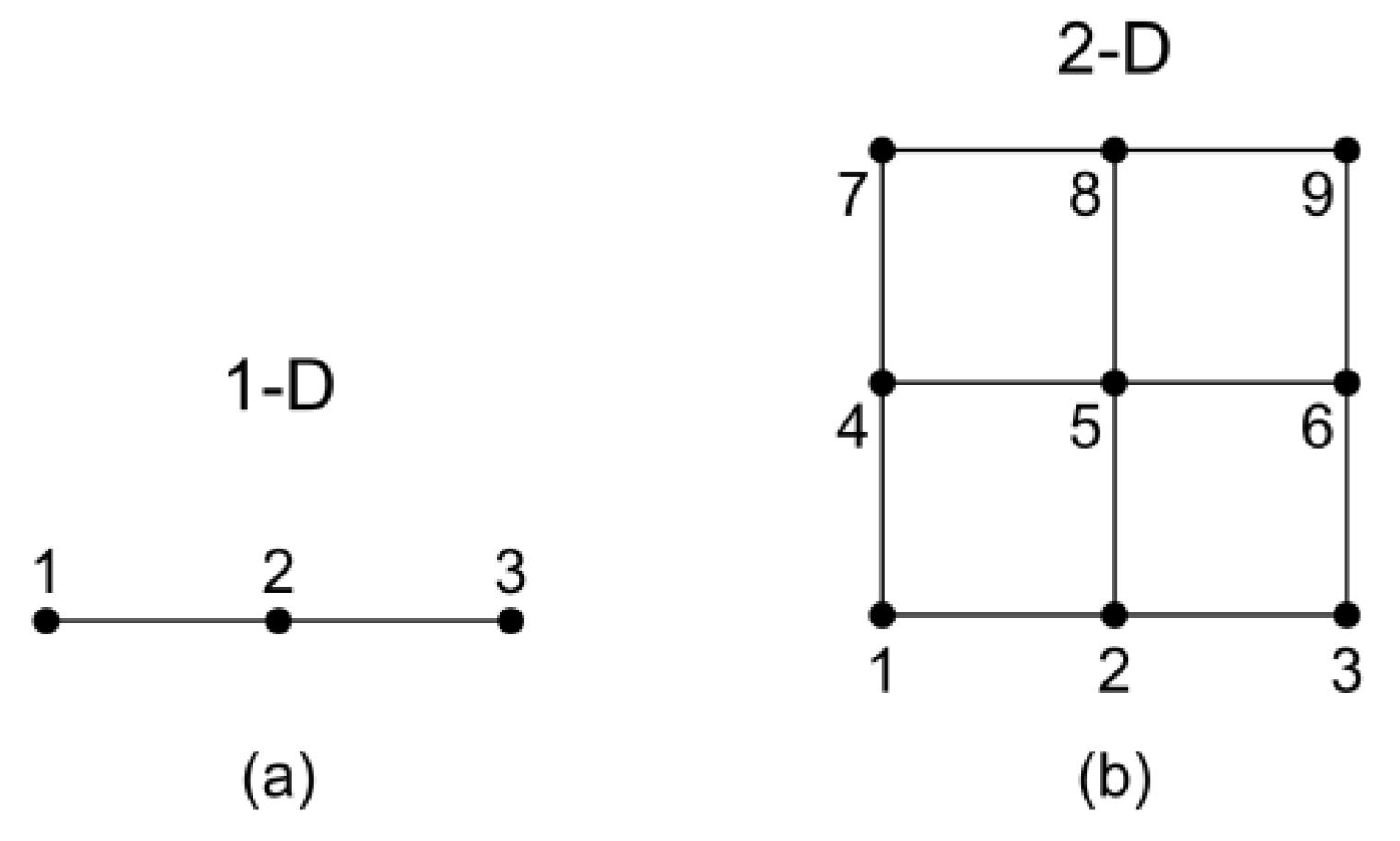
Figure 2.
21-node transfinite element.
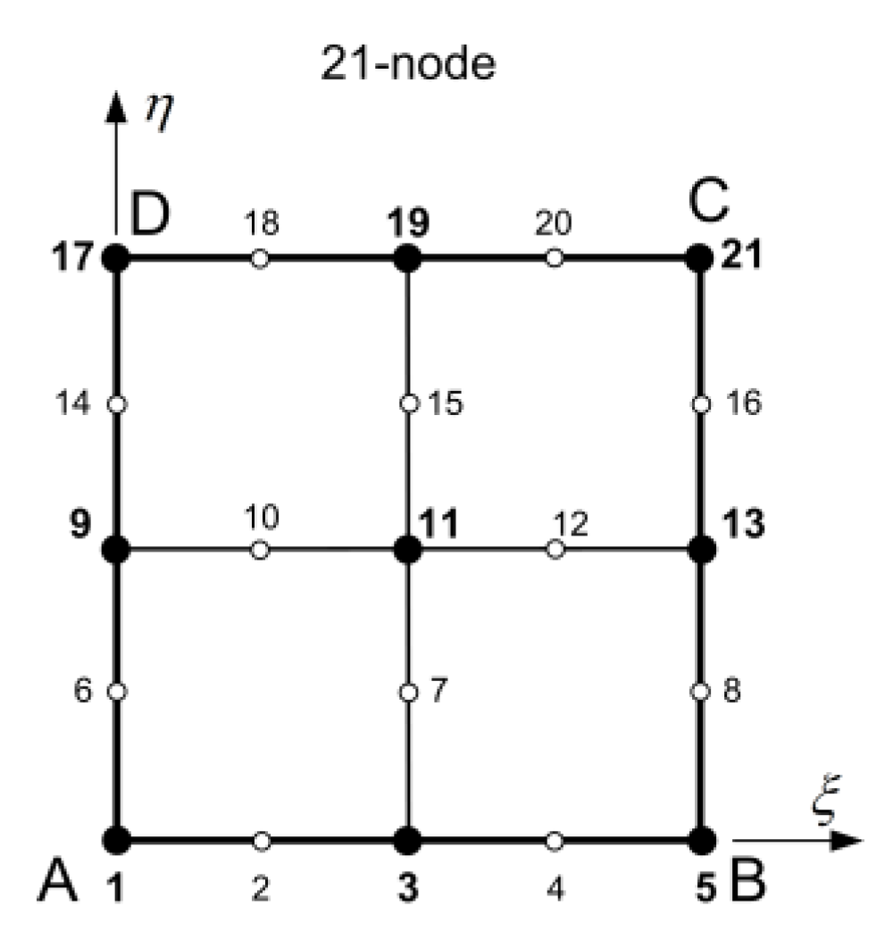
Figure 3.
Shape functions which are associated with the 21-node element.
Figure 4.
T-mesh elements with missing nodes (a) on the boundary, (b) in the interior arranged along vertical isolines, (c) at intersections of isolines.
Figure 4.
T-mesh elements with missing nodes (a) on the boundary, (b) in the interior arranged along vertical isolines, (c) at intersections of isolines.
Figure 5.
Typical higher order macroelements with missing boundary nodes: (a) quadratic, (b) cubic, and (c) quartic.
Figure 5.
Typical higher order macroelements with missing boundary nodes: (a) quadratic, (b) cubic, and (c) quartic.
Figure 6.
Degeneration of (a) quadratic-to-linear, (b) cubic-to-quadratic, and (c) quartic-to-cubic Lagrange polynomials.
Figure 6.
Degeneration of (a) quadratic-to-linear, (b) cubic-to-quadratic, and (c) quartic-to-cubic Lagrange polynomials.
Figure 7.
The bi-quadratic uniform element.
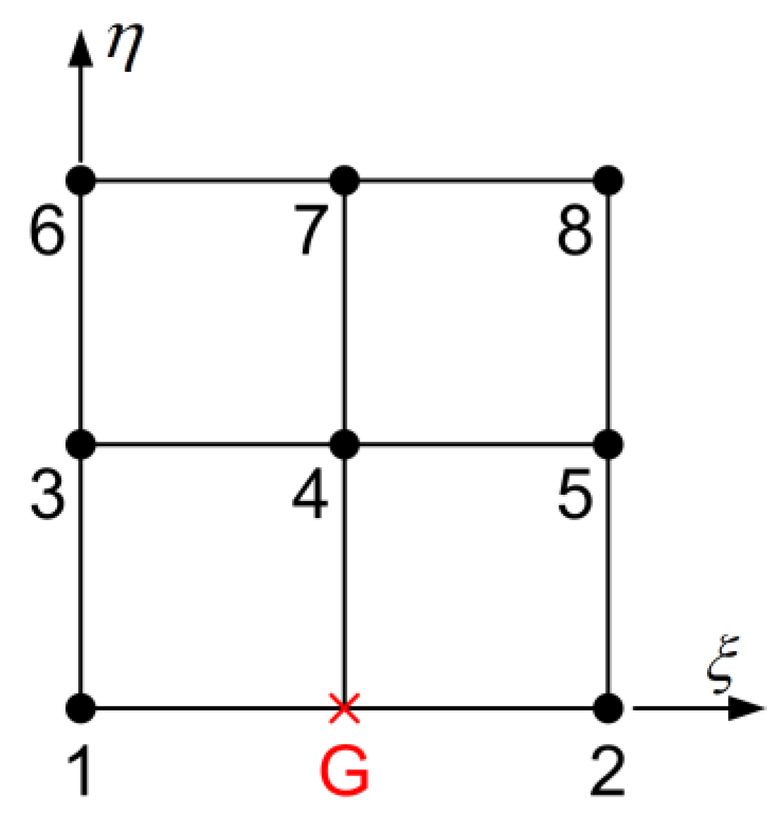
Figure 8.
(a) T-spline like meshes with missing nodes at intersected isolines, and (b) background tensor product grid.
Figure 8.
(a) T-spline like meshes with missing nodes at intersected isolines, and (b) background tensor product grid.
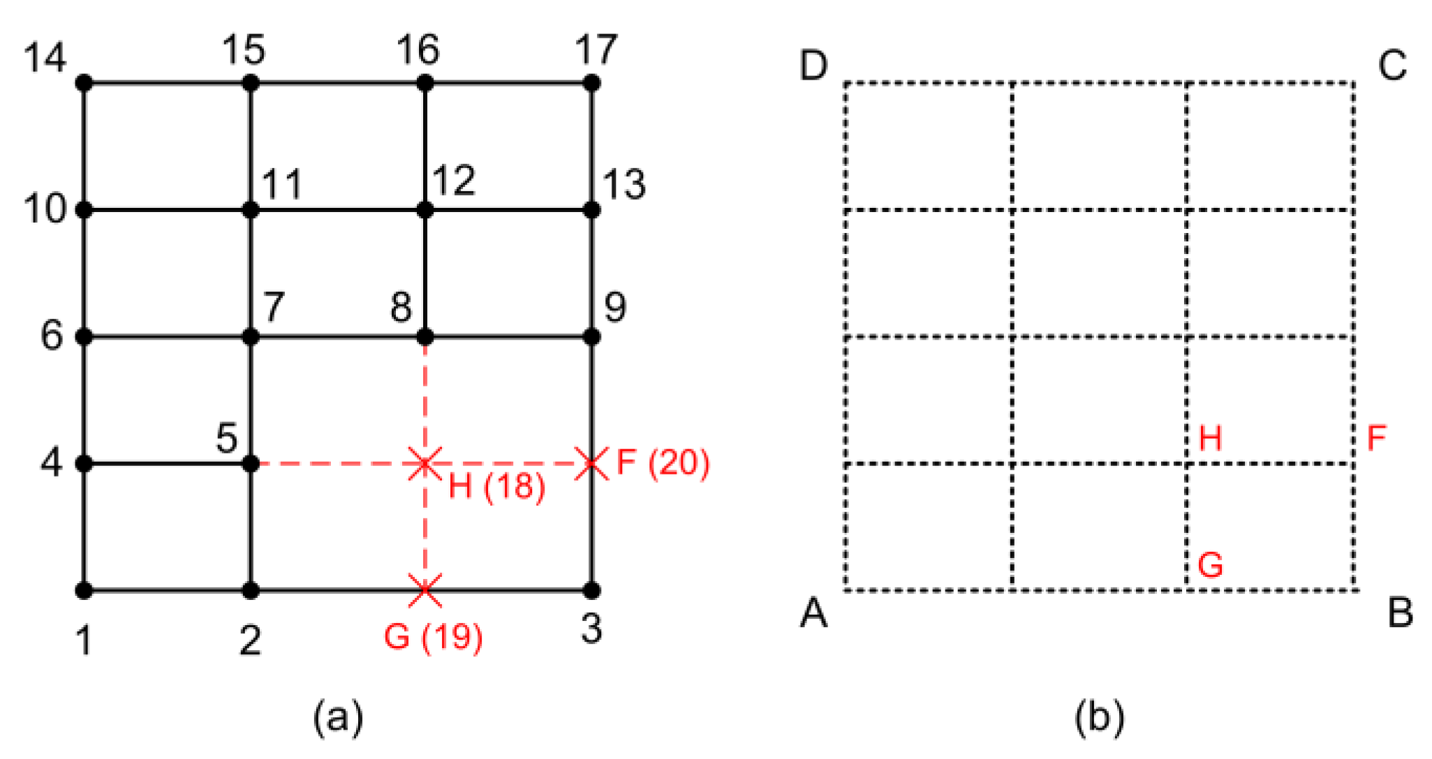
Figure 9.
Shape functions after elimination using Lagrange polynomials: (a) 17-nodes and (b) 18-nodes.
Figure 9.
Shape functions after elimination using Lagrange polynomials: (a) 17-nodes and (b) 18-nodes.
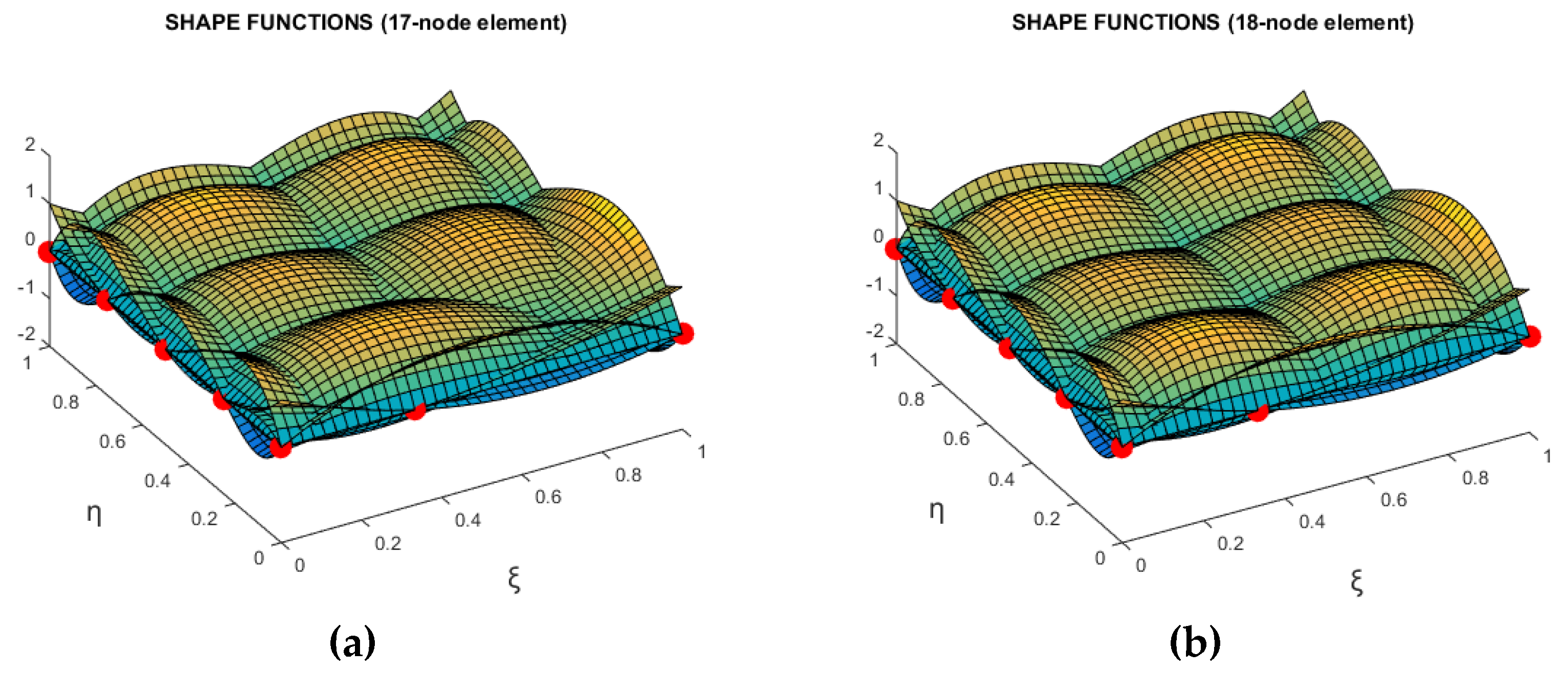
Figure 10.
The 46-node T-element: (a) primary nodes, (b) primary and secondary nodes.
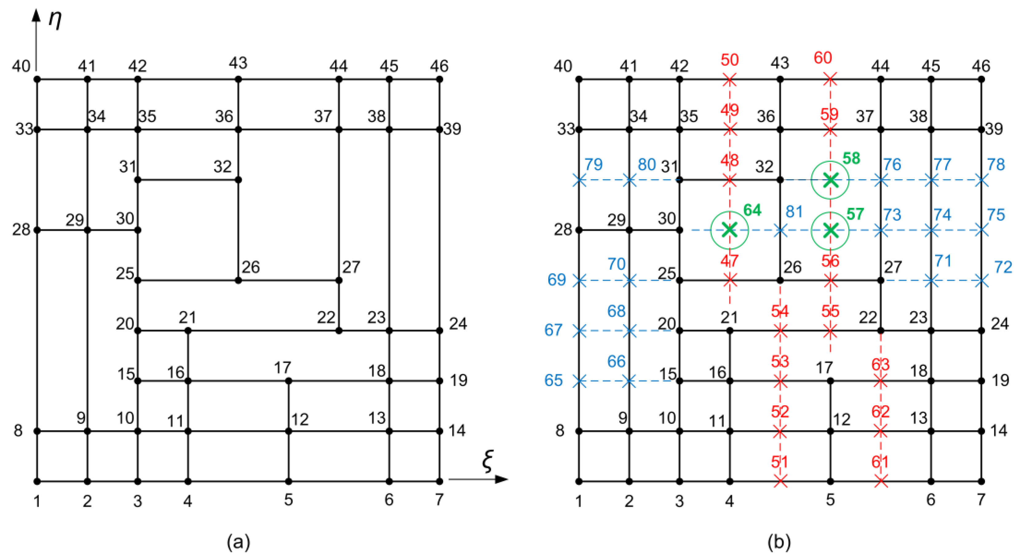
Figure 11.
Shape functions of a 46-node T-element based on Lagrange polynomials and elimination.
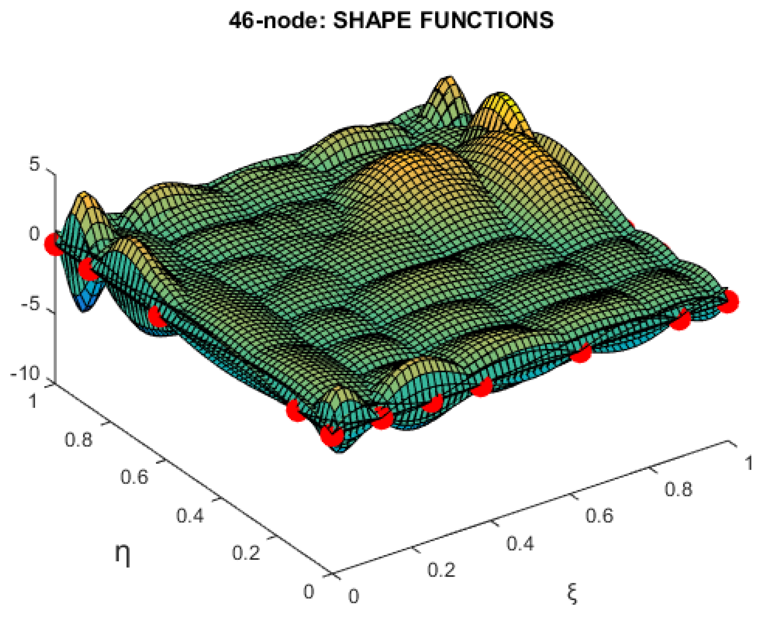
Figure 12.
Square domain: (a) Dimensions and boundary conditions, (b) Tensor-product discretization.
Figure 12.
Square domain: (a) Dimensions and boundary conditions, (b) Tensor-product discretization.
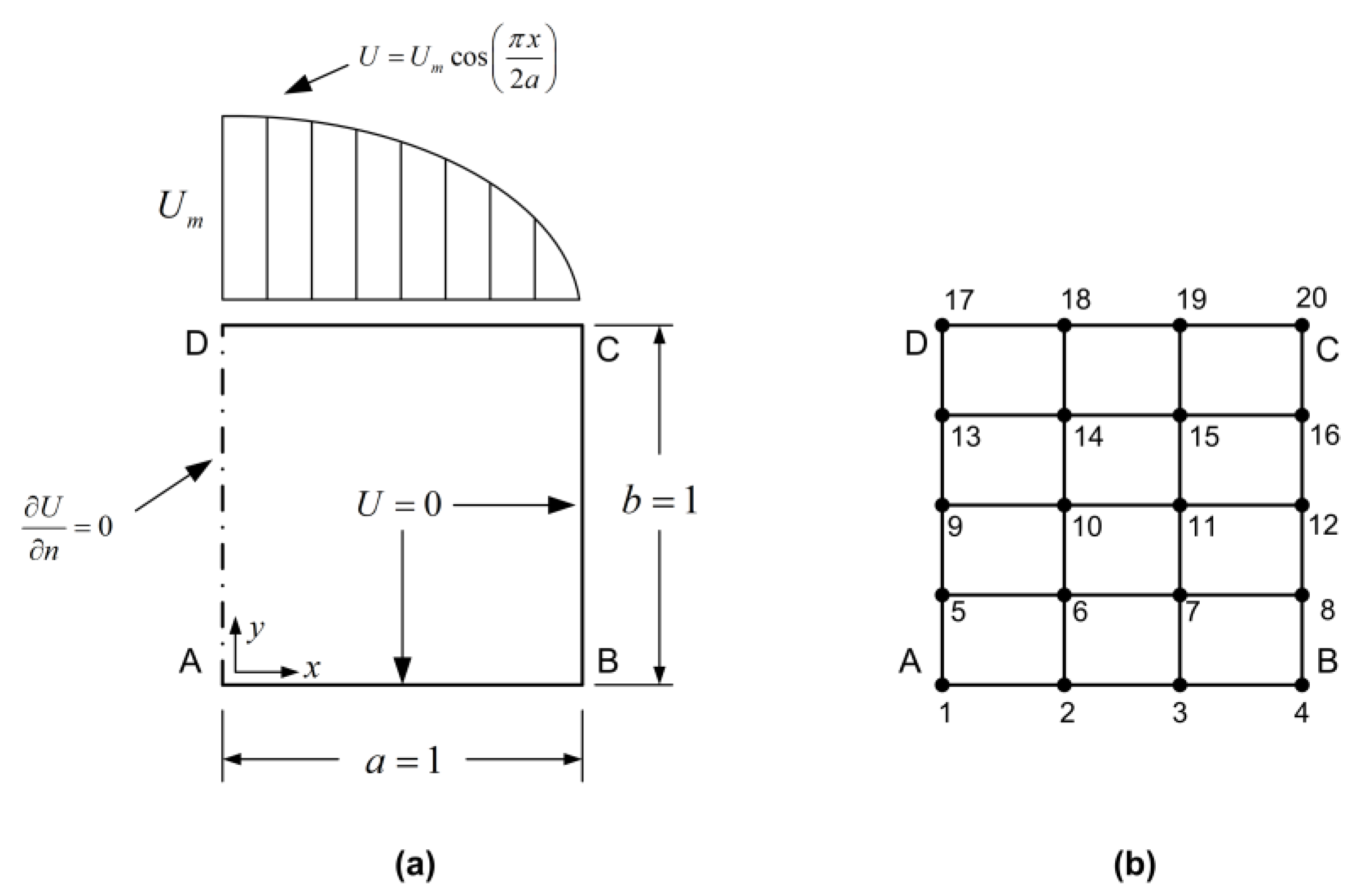

Table 1.
Accuracy of several element types.
| Element type | Figure | L2 error norm (in %) |
| 8node | 4a | 3.2184 |
| Transfinite element (21 DOF) | 2 | 0.0526 |
| Tensor-product (20 DOF) | 6a (and 10b) | 0.2025 |
| 18 nodes | 6a | 0.2035 |
| 17 nodes | 6a | 0.3275 |
| 46 nodes | 8 | 0.0115 |
Disclaimer/Publisher’s Note: The statements, opinions and data contained in all publications are solely those of the individual author(s) and contributor(s) and not of MDPI and/or the editor(s). MDPI and/or the editor(s) disclaim responsibility for any injury to people or property resulting from any ideas, methods, instructions or products referred to in the content. |
© 2025 by the authors. Licensee MDPI, Basel, Switzerland. This article is an open access article distributed under the terms and conditions of the Creative Commons Attribution (CC BY) license (http://creativecommons.org/licenses/by/4.0/).
Copyright: This open access article is published under a Creative Commons CC BY 4.0 license, which permit the free download, distribution, and reuse, provided that the author and preprint are cited in any reuse.


