
Submitted:
18 October 2025
Posted:
20 October 2025
You are already at the latest version
Abstract
This paper presents a unified framework for constructing partially unstructured B-spline transfinite finite elements with arbitrary nodal distributions. Four novel distinct classes of elements are investigated. The first consists of classical transfinite elements reformulated using B-spline basis functions. The second includes elements defined by arbitrary control point networks arranged in parallel layers along one direction. The third features arbitrarily placed boundary nodes combined with a tensor-product structure in the interior. The fourth class comprises classical T-spline elements, characterized by selectively omitted internal nodes that produce sparsely populated, incomplete grids. For all four classes, novel macro-element formulations are introduced, enabling flexible and customizable nodal configurations while preserving the partition of unity property. The key innovation lies in reinterpreting the generalized coefficients as discrete samples of an underlying continuous univariate function, which is independently approximated at each station in the T-index space. This perspective generalizes the classical transfinite interpolation by allowing both the blending functions and the univariate trial functions to be defined using non-cardinal bases such as Bernstein polynomials or B-splines, offering enhanced adaptability for complex geometries and nonuniform node layouts.
Keywords:
transfinite elements
; B-spline functions
; T-splines
; macro-elements
; unstructured grids
; partition of unity
; isogeometric analysis
; finite element method
MSC: 41A10; 41A15; 65N30
1. Introduction
Computational methods have undergone several stages of development and continue to evolve. The progression began with global approximation techniques, such as those introduced by Rayleigh [1], Ritz [2], and the Bubnov-Galerkin method (1913-1915), eventually giving way to more localized approaches like the finite element method [3,4]. Among these developments, transfinite interpolation occupies a particularly important role [5,6]. Initially developed to interpolate the geometry of solid objects and surfaces [7], it soon became apparent that the method could also be used to interpolate scalar and even vector fields within three-dimensional domains. Notably, transfinite interpolation allows the construction of finite elements with differing numbers of nodes along opposing edges or surfaces–without requiring transitional elements. This flexibility extends to the merging of dissimilar domains in two or three dimensions.
An effort to integrate ideas from computer-aided geometric design (CAGD) into analysis methods—such as the finite element, boundary element, and collocation methods—was initiated at the National Technical University of Athens (NTUA) in the summer of 1984, within the research group to which the present author belonged; the first publication appeared later in 1989 [8]. A comprehensive monograph, compiled from approximately 60 journal and conference papers produced by this group, along with an extensive literature review until 2018 (here omitted, for the sake of brevity), is presented in reference [9]. In that monograph, the term macroelement is used to describe an entire patch, whether a surface or a volumetric block. In this framework, although B-splines required domain decomposition at individual breakpoints [8], they were initially regarded more as integration cells than as B-spline elements in the modern sense [10]. Concurrently, similar ideas were being explored by other research groups, as documented in [11,12,13,14,15].
Classical literature on transfinite interpolation (see Refs. [5,6] and references therein) primarily employs linear blending functions, typically Lagrange polynomials. The univariate trial functions defined along the mesh-lines (also referred to as `stations’) are commonly chosen as piecewise linear, piecewise Hermite, or cubic splines. However, in the case of cubic splines, specific implementation details are generally omitted or not fully addressed.
While transfinite interpolation works perfectly well in conjunction with Lagrange polynomials, there is not much experience when it is combined with Bernstein polynomials and B-splines. This is because the former are cardinal polynomials of -type, in the sense they are interpolatory (take the value of unity) along the stations, whereas the latter are not (take a value less than unity). Nevertheless, both sets hold the partition of unity property. This fact has recently sustained the conjecture that transfinite interpolation can be extended in such a way that blending functions can be Bernstein polynomials or B-splines and at the same time they can also be trial functions which interpolate the primary variable U along the stations of the curvilinear patch [16].
Figure 1 presents a collection of multiple classes of transfinite finite elements, starting from the older Coons element (studied in detail in [8,9]) and ending to a multi-layer element. The well-known case of the T-mesh element [17,18,19] —which is a variation of cases (d,e)– is still missing in this collection, but will be extensively discussed later in Section 6.
Recent studies have shown that a direct substitution of Lagrange polynomials with Bernstein polynomials in the final expressions of the shape functions for all types of transfinite elements is feasible, and sometimes yields equivalent results for both polynomial sets. To date, this direct replacement–accompanied by a pointwise agreement between the two polynomial families–has been verified for the following four classes of transfinite elements [20,21]:
- Coons elements (Figure 1a).
- Tensor product elements (Figure 1b).
- Classical transfinite elements of structured pattern (Figure 1c).
- Deformed tensor-product elements (not shown; similar to Figure 1b, but with boundary nodes arbitrarily positioned relative to the orthogonal projection of the internal nodes).
While the primary variable U is a straightforward physical quantity to interpret, the associated discrete generalized coefficients often cause confusion—particularly among engineers rather than applied mathematicians. In general, however, the coefficients form a set of dual quantities corresponding to the nodal values , and the two sets are interconnected through a linear relationship.
First of all, we must report that the expression of tensor-product Bernstein polynomials is not an axiom but a direct sequence of the pre-existed tensor-product of Lagrange polynomials. Clearly, the existing linear relationship between univariate Lagrange and Bernstein polynomials –which share the same monomials– is adequate to offer a mathematical proof for the equivalence between tensor-product Lagrange and tensor-product (non-rational) Bernstein polynomials [9].
Moreover, having established the above explanation for the tensor product of Bernstein polynomials, the interpretation of the tensor-product B-spline follows as a straightforward extension. However, while the rationale behind the tensor-product B-spline is relatively easy to grasp, the same cannot be said for transfinite interpolation, which—even to this day—remains a powerful and versatile tool for constructing novel, large-scale finite elements, as will be demonstrated in the following sections.
The difficulty and delay in advancing the transfinite interpolation method stem from the following issue. Although replacing Lagrange polynomials with Bernstein polynomials is generally straightforward, the challenge lies in substituting the univariate functions along each section (station) orthogonal to the -axis at point . This is due to the fact that all the generalized coefficients associated with the two opposite sides (i.e., and ) of the quadrilateral patch (Figure 2b), which are perpendicular to the station under consideration (thus containing its ends), contribute to the determination of function . Therefore, the classical cardinal blending functions of Lagrange type cannot be directly combined with standard B-splines along the stations, simply because the latter are of global character, that is, it is not possible to interpolate the function through a self-contained expression (trial functions) along a -station. Addressing this incompatibility is the central objective of the present study.
Aiming to address the above issue, a recent preliminary study on transfinite elements has indicated that the classical blending functions –which usually are cardinal functions of [1,0]-type– can be substituted by non-cardinal functions such as Bernstein polynomials and B-splines [16]. The beginning of this inspiration is the 2D analogue of the 1D interpolation using Lagrange polynomials from one side and any other IGA-based functions such as Bernstein polynomials, B-splines, and NURBS. The lowest level of this concept is to think about the quadratic interpolation, which can be implemented either using Lagrange polynomials: or using Bernstein polynomials: . The issue is as follows: It is quite reasonable that the aforementioned three Lagrange polynomials may serve the role of blending (interpolation) functions in the -direction since they fullfil the delta-Kronecker property () and hold the partition the unity property. Therefore, they can accurately represent a constant, a linear, and a quadratic univariate function. Similarly, if the generalized coefficients () are properly chosen each time, the Bernstein polynomials may again accurately represent the same functions (constant, linear, and quadratic).
Clearly, when the blending functions are Bernstein polynomials (or B-splines), the variation in the -direction should be performed in terms of a (supposed existing) univariate function , which for (i.e., on edge ) coincides with the usual generalized coefficients () at points (), respectively. The same holds for a triplet () on the opposite edge at .
The critical point is how to describe the abovementioned function , which is perpendicularly oriented at point . Within the IGA framework, the most easy way is to employ a set of B-spline functions extended in the interval . To this purpose, a safe way is to use clamped splines (for degree : ), whose the end values will be the boundary variable a (and not U). In this way, the previously mentioned difficulty in handling is removed.
The paper is divided into two main parts. The first part focuses on the construction and performance of simplified elements, both classical and newly introduced, including those composed of layers oriented in a single direction. This serves as a pilot study to validate the approach of treating the discrete coefficients as a bivariate function. The second part addresses the well-known T-spline elements.
The present paper is structured as follows: Section 2 introduces the general formulation of transfinite interpolation, employing either Lagrange or Bernstein polynomials, as well as B-splines, for the representation of blending and trial functions. Section 3 describes the construction of classical transfinite elements. Section 4 presents the development of transfinite elements with nodes arranged in parallel layers. Section 5 focuses on elements that combine tensor-product interior nodes with nonuniform boundary node placement. Section 6 addresses T-spline elements of increasing complexity. Section 7 discusses software-related aspects. Section 8 provides numerical results for all models, Section 9 briefly refers to possible implementation of the collocation method as an alternative, and Section 10 offers a detailed discussion. The paper is supplemented by seven appendices.
2. Transfinite Interpolation Using B-Splines
2.1. Terminology
In classical computer-aided geometric design (CAGD) [22], the term blending function typically refers to univariate interpolation functions used in a specific parametric direction. For instance, consider a Coons patch defined over the quadrilateral , with the origin at vertex A and the -axis oriented along edge (Figure 2b) [2]. The blending functions and interpolate between the boundary functions ) and ) in the -direction.
This usage of the term differs from its meaning in T-spline literature, where blending functions are often synonymous with basis functions [18]. In this paper, we adopt the classical interpretation: the term blending function will refer specifically to the interpolation functions used in Coons or Gordon patch construction, as adopted in Refs. [2,22,2,22]. Throughout the present paper, the term basis functions will be used uniformly for both B-splines/NURBS and T-splines.
A second key concept in classical transfinite interpolation theory–as well as in finite element methodology, as emphasized in Zienkiewicz’s seminal work–is that of trial functions [2]. In the present study, this term refers to univariate functions defined along boundary edges, or more generally, along horizontal and vertical mesh-lines (stations) within the domain.
A third issue concerns the use of the terms transfinite element and macroelement. In this paper, these terms are used synonymously to refer to the parametric patch defined over the domain . Regardless of the choice of blending or trial functions, the resulting basis functions share the same closed-form expression. The main difference lies in the interpolation approach: Lagrange and Bernstein polynomials perform global interpolation over the entire patch, whereas B-splines use piecewise polynomial interpolation between breakpoints, which define the integration cells. Naturally, in the B-spline formulation, not all degrees of freedom (DOFs) are active within every integration cell. However, to maintain a uniform treatment across all three cases (Lagrange, Bernstein, and B-splines), we do not emphasize this distinction.
2.2. State of the Art
The general expression of transfinite interpolation for 2D patches is given in [2]:
where and are projectors of the quantity U along the parametric axes and , respectively, and is the corrective projector, defined as the tensor product of nodal values at the intersections of the coordinate stations.
It is well known that, for vertical stations passing through , and for horizontal stations located at , we construct univariate blending functions and of degrees m and n, respectively (assuming Lagrange polynomials are used). Based on the univariate functions and defined along the vertical and horizontal stations, respectively, we obtain:
On the other hand, along each station, the variable is interpolated using trial functions , where the variable s denotes either of the parametric directions or , as follows:
Here, the overbar denotes a prescribed value of a given parameter ( or ) along the corresponding station—vertical for or horizontal for . In general, the number of nodes ( or ) along a station may differ—either smaller or greater—from the number of stations in the same direction. The case of equality (e.g., in a tensor-product configuration) is also included.
Henceforth, for brevity, the notation following each projector is suppressed; for example, is written simply as , and similarly for the others.
2.3. Extension of the Projectors Using Bernstein Polynomials
The classical interpretation of the well-known projectors (, , and ) is founded on their application to the primary variable , in accordance with the use of Lagrange polynomials as blending functions and , as presented in Ref. [2]. It is well established that Coons interpolation represents a direct extension of one-dimensional linear interpolation to two-dimensional domains [9]. Similarly, classical transfinite (Gordon) interpolation generalizes one-dimensional polynomial interpolation to bivariate patches. Since one-dimensional polynomial interpolation can be formulated using either Lagrange or Bernstein polynomials [23], it follows that the classical projectors may likewise be expressed in terms of Bernstein polynomials.
The above claim will be demonstrated—in full detail for the first time—for one projector, namely ; the same holds for the remaining ones. Let us consider three points , , and on a parametric curve and the associated values , , of a univariate function (Figure 2a). These can be interpolated in terms of the nodal values (, , ), using the quadratic Lagrange polynomials , , :
Alternatively, the same points can be interpolated in terms of the generalized coefficients (, , ) using the quadratic Bernstein polynomials , , and :
The above equations can be extended from one to two dimensions, beginning with the projector , in which the nodal values (, , ) are replaced by univariate functions (, , ), as illustrated in Figure 2b:
Similarly, in terms of Bernstein polynomials, the same projector is expressed in the form of a separation of variables, as follows:
Of course, a significant distinction exists between the two formulations presented above. The Lagrange interpolation (Eq. (9)) is a local scheme applied to univariate functions that directly represent the primary variable at discrete stations located at . In contrast, the Bernstein interpolation (Equation (10)) is a global approach, involving univariate functions constructed from generalized coefficients.
This implies that while the interpolation of the primary variable U is straightforward and intuitive, the corresponding interpolation of the coefficient a is less direct. Nevertheless, the coefficient a embodies a definitive quantity that, in essence, is not fundamentally different from the variable U. For instance, in the case of quadratic interpolation, we observe:
Therefore, if—for instance—the extreme values are equal (i.e., ), the coefficient corresponds to . This implies that a duplication of the associated basis function can be employed to ensure that effectively represents the actual variable .
2.4. B-Splines Projectors
A comprehensive investigation into the use of B-splines as blending functions was recently presented in Ref. [16], although the treatment therein was primarily speculative. In contrast, the methodology introduced in this paper adopts a more rigorous framework and may be interpreted in analogy with a function of separated variables, namely , where the role of is assumed by the function , which is intrinsically linked to the generalized coordinates.
In general, the number of mesh lines (stations) along each parametric direction determines the length of the corresponding knot vector used for the blending functions. Likewise, the number of control points defined at each station governs the length of the associated knot vector for the trial functions. Further clarification and illustrative examples will be provided in the subsequent sections.
3. Construction of Classical B-Spline Transfinite Elements
A representative transfinite element , comprising 113 control points, is depicted in Figure 3d. It can be observed that the element is structured with four horizontal and five vertical stations (including the boundary edges), upon which the control points are distributed. The horizontal set of stations is oriented perpendicular to the -axis and positioned at , while the vertical set is oriented perpendicular to the -axis and located at .
Based on the aforementioned station configuration, the blending functions in the -direction may be chosen as Lagrange or Bernstein polynomials of degree 4, corresponding to five station values. Similarly, in the -direction, the blending functions may be Lagrange or Bernstein polynomials of degree 3, associated with four station values.
Alternatively, when employing cubic B-splines, the -direction can be represented using the knot vector
which corresponds to five distinct station values and ensures continuity. In the -direction, the blending functions may be defined by the knot vector
which corresponds to four station values and yields Bernstein polynomials of degree 3.
In all cases, the construction of the knot vectors for the blending functions must guarantee that the number of control points aligns with the number of stations, thereby ensuring proper interpolation and continuity across the transfinite element.
Under these conditions, the three projectors defined by Eqs. (2) through () are now reformulated in terms of B-spline-based blending and trial functions, where the trial functions are associated with the generalized coefficients .
Upon further elaboration, it is found that the Boolean sum in Equation (1) yields a total of 113 basis functions. These functions can be categorized into two distinct groups, as follows:
- (1)
-
Nodes at section intersections (including corner nodes A, B, C, and D), for example:In this expression, denotes the second blending function in the -direction, corresponding to the second vertical station where node 69 is located. Likewise, refers to the 9th B-spline basis function in the -direction, as node 69 is the 9th node from the bottom. The same logic applies to the remaining terms.
- (2)
-
Intermediate nodes on single stations, for example:Here, is the third blending function in the -direction, indicating that node 71 lies on the third horizontal station. Similarly, represents the 7th B-spline basis function in the -direction, as node 71 is the 7th node from the left boundary.
By classifying the 113 degrees of freedom into the two aforementioned categories, the complete set of basis functions can be systematically constructed. Specifically, 20 of these functions—corresponding to the black-filled circles in Figure 3d—are composed of three terms, as exemplified by Equation (12), and reflect contributions from all three projectors. The remaining 93 functions—associated with the white-filled circles—are expressed as simple tensor products, as illustrated in Equation (13).
With respect to the blending and trial functions, the formulations presented above are of general applicability. In the following sections, several alternative modeling approaches will be examined and compared.
3.1. Model-1: Lagrange Polynomials
As a representative example, we consider the following configuration (Figure 3d):
- (1)
- Lagrange polynomials of degree and are employed as blending functions in the - and -directions, respectively.
- (2)
- Lagrange polynomials of degree and are used as trial functions in the - and -directions, respectively.
For this Model-1 setup, the resulting bivariate global shape functions are depicted in Figure 4a. Notably, elevated function values are observed along the vertical edges, indicating localized influence. Furthermore, the constructed basis satisfies the partition of unity property:
3.2. Model-2: Mixed Scheme
In this model, the blending functions are retained from Model-1, namely Lagrange polynomials of degree and in the - and -directions, respectively. For the trial functions, however, we adopt the classical natural cubic cardinal B-splines, which are directly associated with the nodal values U. This approach mirrors the behavior of Lagrange polynomials in Model-1, thereby eliminating the need for generalized coefficients .
This formulation is particularly well-suited to uniform nodal distributions with single knots and facilitates direct comparison with Model-1. It is worth noting that this type of spline interpolation—natural cubic B-splines—was widely used during the mid-1980s (see [24], among others).
In brief, the knot vector for the trial functions in the -direction consists of 23 entries:
which generates 19 control points. From these, 17 univariate cardinal trial functions are constructed, corresponding to the 17 nodal points along the horizontal stations.
Based on the formulations in Eqs. (12) and (13), the graphical representation of the resulting 113 basis functions is shown in Figure 4b. These basis functions have been verified to satisfy the partition of unity property:
and exhibit unity as their upper bound.
Further details regarding the construction of the cardinal univariate set of natural cubic B-splines can be found in Ref. [9], and relevant implementation code is provided in Appendix A.
3.3. Model-3: Cubic B-Splines
This model closely aligns with the current state-of-the-art practices in Isogeometric Analysis (IGA), where classical B-splines (de Boor formulation) or NURBS are commonly employed. In this framework, B-splines are utilized for constructing both the blending and trial function sets. Classical clamped splines are adopted, reflecting the fact that for a polynomial degree p, the minimum number of control points is in the case of Bernstein polynomials, whereas for pure B-splines, the condition must be satisfied.
Within this context, the 113-node transfinite element illustrated in Figure 3d should be interpreted as an index space rather than a physical nodal layout. In Models 1 and 2 (see Sects. Section 3.1 and Section 3.2), each of the 113 nodal points was directly associated with a unique bivariate shape function linked to a nodal value , leaving no ambiguity in the trial function definition.
Assuming that the 17 points along each horizontal station are treated as single breakpoints, it is well known that the corresponding number of control points becomes 19. Conversely, if only 17 control points per horizontal station are desired, one must define 15 breakpoints, resulting in 14 knot spans in the -direction. The associated knot vector is then given by:
Similarly, to obtain 13 control points in the -direction (based on 11 breakpoints and 10 knot spans), the corresponding knot vector is:
The graphical representation of the resulting basis functions is shown in Figure 4c.
4. Construction of Multi-Layer Finite Elements with Nodes Arranged in Parallel Layers
We now examine multi-layer finite elements containing internal nodes, where the number of nodes per station (i.e., per parallel layer) may vary. Such configurations arise when nodes—both internal and boundary—are aligned along unidirectional stations, for instance, distributed horizontally, as depicted in Figure 1e.
4.1. Unidirectional Multi-Layer Transfinite Lagrange and Bernstein Elements
The unidirectional analog of Equation (10), corresponding to the configuration shown in Figure 1e where all five stations are parallel to the horizontal -axis, is given by the following projector:
In this formulation, the approximation function is expressed as . Each component function , for , can be represented using clamped B-splines. The corresponding knot vectors are constructed such that the number of control points matches the number of nodes shown in Figure 1e.
It is important to note that the interpolatory nature of these B-splines—exhibiting unit values at the endpoints of each horizontal station (i.e., at and )—does not introduce any complications. This is because each function is multiplied by a non-cardinal blending function , analogous to the behavior observed in one-dimensional problems.
For instance, if is a constant function, the clamped B-spline basis will represent it exactly. This observation underscores that the value of U is influenced by all coefficients a within the patch, a property particularly relevant for Bernstein polynomials. However, in the present formulation, the focus is on the coefficient functions rather than the potentially problematic direct interpolation of U along each horizontal station.
A previous report, Ref. [16], proposed the conjecture that transfinite interpolation can be effectively employed using a wide variety of blending functions, provided that the partition of unity condition is satisfied and the function set is complete. Within this framework, not only cardinal Lagrange polynomials but also non-cardinal blending functions—such as Bernstein polynomials and B-splines—have been successfully explored.
Furthermore, in the context of trial functions, any well-established univariate functional basis may be considered a viable candidate for use within numerical analysis modules, including Galerkin and collocation methods. This flexibility allows for the integration of diverse approximation schemes while maintaining consistency with the underlying transfinite interpolation principles.
Let us consider a class of transfinite elements with unidirectional nodes, as shown in Figure 5. Let us focus on the 12-node element (Figure 5a). Replacing Equation (9) by the vertical projection , and then expressing the involved univariate functions in terms of Lagrange polynomials of variable degree p associated with each horizontal station (layer), we obtain the following set of bivariate global shape functions:
Next, replacing Lagrange polynomials with their Bernstein counterparts, or alternatively applying the projector defined by the analog of Equation (18) (including three terms associated with the three layers in Figure 5a) by expressing the involved univariate functions in terms of Bernstein polynomials, we obtain the following set of non-negative basis functions:
The shape functions based on Lagrange polynomials (Equation (19)) are illustrated in Figure 6a, while the basis functions corresponding to Bernstein polynomials (Equation (20)) are shown in Figure 6b. This element is not provided for B-spline interpolation, as it contains too few nodes to support such a representation.
4.2. Unidirectional Transfinite B-Spline Elements
Below we focus on the 18-node element shown in Figure 5b. The characteristic of this element is that—in addition to the four edges—it includes two internal stations which are both oriented in the -direction (horizontal stations), and thus (as also happened with the 12-node element) the only non-zero projector among the three is , i.e., . Since the total number of horizontal stations is 4, there is no cubic B-spline to cover this case (unless we select quadratic B-spline), and therefore we resort to cubic Bernstein polynomials (hybrid scheme), as follows:
- (1)
- The blending functions in vertical ()-direction were taken as cubic Bernstein polynomials, , where .
- (2)
- The base 1-2-3 was modelled by quadratic Bernstein polynomials: .
- (3)
- The second layer, with nodes 4-5-6-7, was modelled by cubic Bernstein polynomials, .
- (4)
- The third layer, with nodes 8-9-10-11-12, was modelled as a set of five cubic B-splines, , with knot vector .
- (5)
- The fourth (top) layer, with nodes 13-14-15-16-17-18, was modelled as a set of six cubic B-splines, , with knot vector .
Writing a projector similar to that of Equation (18), in conjunction with four parallel layers (stations) at , we obtain the following basis functions:
Obviously, the same form as Equation (21) holds when the blending and trial functions are all of Lagrange type or all of Bernstein type. For all these three cases, the graphs of the basis functions are shown in Figure 7.
Regarding the estimation of the stiffness matrix of the 18-node transfinite element in Figure 5b, the fully-Lagrange and the fully-Bernstein models require an integration scheme of Gauss points in the - and -directions, without local support. This is because the maximum polynomial degrees per single basis function are and , respectively, and thus the multiplication in the integrand will contain terms up to . In contrast, for the same patch, the piecewise cubic B-spline interpolation requires integration cells (i.e., 30 B-spline elements, as they have been called in standard IGA [10]) with Gauss points per element (i.e., a total of 480 integration points, however with local support).
Note: When the number of parallel sections increases to 5 (and thus the number of nodes becomes 25, as shown in Figure 5c), the 25-node transfinite element may be handled using blending functions of B-spline type, based on the knot vector . Moreover, regarding the 32-node element made of 6 horizontal sections (partially non-uniform, as shown in Figure 5d), results and discussion are given in Section 8.1.2.
5. Finite Elements Featuring Tensor-Product Interior Nodes and Nonuniform Boundary Node Placement
This is a class of elements (the third in the present paper) in which the boundary nodes are placed arbitrarily, and the interior is populated using a tensor product grid of internal nodes. A common rule of thumb is to choose the number of internal points in each direction (m or n) based on the average number of intermediate nodes on opposite edges. This class of elements has previously been formulated using Lagrange polynomials as both blending and trial functions [16,20]. In the present paper, the methodology is extended by introducing B-splines as an alternative choice for both blending and trial functions.
5.1. 27-Node Transfinite Element
As an example, we consider a 27-node transfinite element, in which the four edges are uniformly divided into 4, 3, 6, and 5 segments, respectively, as shown in Figure 8. For this configuration, we can construct at least three different formulations (blending and trial functions) of the transfinite element as follows:
- Lagrange polynomials;
- Bernstein polynomials.
- B-splines
Regarding Lagrange and Bernstein polynomials, the associated polynomial degrees per edge are as follows: , , , and . The internal nodes form a uniform tensor product pattern of scheme (nodes 19 to 27 in Figure 8), which means that the degree of the blending functions is (between edges and internal nodes, four node spans per direction are created). Therefore, this element consists of 18 boundary and 9 internal nodes.
The above 27-node B-spline element is defined by a regular tensor-product arrangement of internal nodes in a grid. However, each of the four edges features a different discretization: edge contains 5 control points, edge has 4, edge includes 7, and edge consists of 6 control points. For clarity, node numbering starts from the boundary and proceeds to the interior. The internal grid lines intersect edge at points , edge at , and the top edge at . Notably, in this example, the bottom edge is defined such that its intermediate points coincide exactly with the orthogonal projections of the internal nodes (19 to 27) onto it, for the sake of alignment and illustrative symmetry.
For this element, the transfinite interpolation (Equation (1)) consists of the following projectors (the auxiliary points, which are necessary to define the projectors, are denoted in red ×):
also
and
Furthermore, if we consider that for either we have:
the substitution of Equation (22) to Equation (25) into the Boolean sum given by Equation (1) cancels all the auxiliary red-colored terms, and thus the bivariate function is approximated by:
The above model offers flexibility in the choice of the univariate blending and trial functions. Therefore, we can proceed as follows:
- (1)
- The five blending functions per direction, horizontal or vertical, can be ensured by the knot vector which guarantees five control points.
- (2)
- The trial functions along the edge are chosen to match the blending functions in the -direction, since all associated control points are orthogonal projections of the internal points onto this edge.
- (3)
- The four control points along the edge are ensured by the knot vector , which effectively corresponds to a set of four Bernstein polynomials of degree 3.
- (4)
- The seven control points along the edge are ensured by the knot vector .
- (5)
- The six control points along the edge are determined by the knot vector .
Under these assumptions, the 27 basis functions are defined as follows:
Regardless of the element type, the formulas for the shape or basis functions remain identical. According to the Boolean sum formulation, the corner nodes on the bottom edge—discretized identically to the interior—are not influenced by the blending functions, whereas the corner nodes on the top edge are affected.
For instance, using cubic B-splines for the blending functions:
and also employing cubic B-splines for the trial functions along the edges, the resulting set of bivariate basis functions is:
The graph of the 27 basis functions , which are involved in Equation (26) and described by Equation (27), is shown in Figure 9. It has also been verified that the functional set satisfies the partition of unity property, i.e.,
It is noted that the basis functions can be categorized into three groups as follows:
- (1)
- Internal nodes: Defined by a simple tensor product of blending functions.
- (2)
- Intermediate boundary nodes: Constructed as local tensor products of trial functions along the edge and blending functions in the perpendicular direction.
- (3)
- Corner nodes: Formulated using a Boolean sum of three terms. Two terms correspond to projectors perpendicular to the edges connected to the corner node, while the third term is a tensor product of the associated blending functions, serving as a correction.
6. Handling T-Spline Elements
Although the previous sections referred to T-spline-like elements, this section systematically addresses the classical T-spline element. This element is defined by a T-index, which includes m knots in the -direction and n knots in the -direction of the parametric domain , where .
In the common case of a cubic T-spline, the anchors of the element form a tensor-product grid of potential anchor positions. However, some of these anchors may be missing, depending on the local refinement and topology of the T-mesh.
6.1. The Two Approaches
In general, two equivalent approaches can be developed, as follows [16]:
- (1)
- Transfinite interpolation
- (2)
- Background tensor-product
Similar techniques have previously been applied in conjunction with Lagrange polynomials [21] and Bernstein polynomials [20]. In those cases, it was possible to globally eliminate the degrees of freedom (DOFs) associated with the missing nodes in the tensor-product grid.
Since the central approach of this paper is to first control the stations (sections or isolines) and then blend them, it is immaterial whether the focus is on a boundary edge or an internal station (inter-boundary). Naturally, when operating along a boundary edge (e.g., edge ), the computations are strictly one-dimensional, as each edge is independent of the remaining data associated with the patch .
In contrast, knot insertion in the interior of a cubic T-spline typically affects a surrounding region spanning two steps in each direction. However, in our numerical scheme—regarded as a first approximation—this influence is intentionally neglected.
6.2. Transfinite Interpolation Versus Tensor-Product
Transfinite interpolation applies to cases where each internal node lies on a single line—either horizontal or vertical—so that the associated degree of freedom (DOF) is involved exclusively in either the or the projector, respectively. However, if the internal point lies at the intersection of a horizontal and a vertical line, an alternative approach must be adopted—for example, by taking the average of the two lines.
As an example, let us consider a T-mesh with a maximum of 9 control points per section (Figure 10). Suppose that two knots are missing on the bottom edge , and thus the function is approximated as a B-spline associated with 7 univariate functions:
as illustrated by the black-colored nodes 1 to 7 in Figure 10b (red-colored nodes 77 and 78 at are missing). Since this set of B-splines is involved in the projector , it follows that the associated bivariate basis functions are given by:
The seven B-spline functions along the edge are also plotted as solid lines in Figure 11.
The same result along the edge can also be obtained via an alternative approach. We virtually assume that all nine control points—fully occupying the nine uniformly spaced positions—contribute to the interpolation of the primary variable U along the edge . Furthermore, we consider this complete configuration as resulting from a previously incomplete one, following knot insertion at the previously missing locations: .
The relationship between the assumed initial (incomplete) and the final complete configuration is detailed in Appendices Appendix B and Appendix C. More specifically, the complete set ( of size ) is related to the incomplete set ( of size ) through the transformation matrix , as follows:
It is noted that the matrix was obtained by calling the subroutine cited in Appendix C twice. The first call corresponds to the insertion of the knot at , resulting in the transformation matrix , while the second call corresponds to the insertion of the knot at , yielding the transformation matrix . The cumulative effect of inserting both knots leads to the overall transformation matrix , and consequently, its transpose is given by .
Substituting Equation (29) into the full B-spline sum expansion, we obtain:
Obviously, Equation (30) dictates that the set of B-splines based on the seven control points (incomplete system: ) is a linear combination of the basis functions of the complete system (), which is defined by the product of a row vector and a transformation matrix:
6.3. Application of Knot Insertion Functions on the Entire Boundary of T-Spline
The above procedure is straightforward and can be extended from edge to the remaining boundary edges: , , and . From a numerical standpoint, substituting the incomplete basis with the complete one does not require matrix inversion, but only a simple matrix multiplication: , where denotes the incomplete vector of basis functions, is the transformation matrix, and is the complete vector associated with the tensor-product basis. Since the background tensor-product basis satisfies the partition of unity property, the same property holds after the substitution described by Equation (A19) in Appendix B.
Let us now complete the discussion of Figure 10b, which illustrates a T-spline patch composed of 76 control points. This configuration is derived from a full tensor-product grid of 81 points, with five control points missing from the boundary. In this extreme case, the patch interior is fully populated, while the boundary is incomplete—lacking five control points (indicated by red crosses in Figure 10b and highlighted in red below) required to complete the full tensor structure. By considering the 76 actual (or primary) control points—shown in black—and the five missing (secondary) ones, we conceptually reconstruct a complete tensor-product grid in the background. The expansion of the primary variable over this virtual tensor-product grid (in which the updated variables—after elimination using Equation (29) and subsequent steps—are denoted by the superscript `tp’) is then expressed as:
(29)
The main concept is that the basis functions associated with the 76 primary DOFs of this T-spline element will be produced by eliminating the red-colored secondary DOFs. This idea has been successfully applied in conjunction with Lagrange polynomials, where the values of the incomplete polynomials were calculated at the missing points and then substituted into virtual polynomials of higher degree in the tensor product [21], in a global manner for the entire station under consideration.
However, in the context of B-splines, if we wish to preserve the same polynomial degree, a different technique is required to substitute the red-colored variables.
Since the tensor-product configuration is fully controlled and the associated basis functions are standard B-splines, it can be considered as a state produced by virtual knot insertion into a coarser mesh—namely, the given T-mesh (defined by its index space). In this example, we must eliminate two DOFs along edge , one DOF along edge , and two DOFs along edge .
In total, the model includes 76 primary nodes and 5 auxiliary (secondary) nodes—located on the boundary—which merely complete (or close) the tensor-product structure in the background.
More specifically, the treatment of edge has already been discussed in Equation (29).
Similarly, for the edge we have:
Since the top edge is complete, we keep it intact and proceed to the final edge , for which we have:
Substituting the three sets of equations—Equation (29), Equation (32), and Equation (33)—each corresponding to an active edge, into the tensor product defined by Equation (Section 6.3), and performing factorization, we obtain:
where the basis functions are given by:
In Equation (35), we have assumed that through represent the B-splines for , while through correspond to the B-splines for . The symbol E is also consistent with the interpretation of blending functions. However, the tensor formulation—whether based on Lagrange, Bernstein, or B-spline functions—is fundamentally governed by one of the three projectors: , , or , as thoroughly discussed in Ref. [9].
The graph of these basis functions is shown in Figure 12. One may observe that:
- (1)
- None of the degrees of freedom (DOFs) associated with the top edge are affected, as this edge is fully occupied.
- (2)
- Among the 76 DOFs, the only affected ones are those associated with nodes . All of these nodes lie on the affected boundary, comprising the three edges: , , and .
- (3)
- Although node 2 lies on edge , it is not affected by the nearest inserted knot at point `77’, since it is located three units away.
- (4)
- None of the interior tensor-product DOFs are influenced by the coarse mesh along the boundary.
- (5)
- The shape and its parametric representation remain unchanged.
- (6)
- The partition of unity is satisfied a priori for all :and therefore, no normalization is required.
- (7)
- The error for the tensor-product element (81-node) is .
- (8)
- The error for the 76-node element was found to be , which is approximately double that of the tensor-product element.
6.4. Treatment of Internal Nodes
Regarding the internal nodes, any missing knot can be treated in an analogous manner to the boundary case. The key difference is that when a gap is filled by inserting a knot, the influence may extend in two parametric directions. The simplest scenario occurs when the missing knot affects only a single station—e.g., a horizontal line. This concept is directly applicable when using Lagrange or Bernstein polynomials.
Let us consider a simple case inspired by Ref. [25]. Specifically, three internal vertices are missing along three horizontal lines at , corresponding to the parametric positions , as illustrated in Figure 10c. For each of these missing vertices, we define the following transformation matrix:
so that the tensor-product degrees of freedom (DOFs), denoted by , are related to the actual ones, , through the transformation
In more detail, we impose the following sets of constraints for each missing internal vertex:
In Eqs. (38)–(40), the superscript “tp” (standing for tensor product) in indicates that the k-th degree of freedom (DOF), shown in Figure 10c and subject to the constraint, represents the final value after the elimination process. This final value is subsequently employed in the expression of the initial tensor-product form, whereas the variables on the right-hand side correspond to the values prior to elimination.
6.5. Intersected Isolines
While handling missing vertices along the isolines of a T-mesh is relatively straightforward—as demonstrated in Section 6.4—complications arise when a missing vertex is located at the intersection of two isolines. In such cases, the numerical results may vary depending on the choice of isoline along which the elimination is performed.
Extensive numerical experimentation suggests a more robust strategy: perform the elimination independently along both isolines and then take the arithmetic mean of the two results as the final expression for elimination.
A simple test case is illustrated in Figure 14, where the central node (located at ) has been omitted from the tensor-product grid of 81 nodes.
The imposed constraints are:
Regarding the horizontal -direction:
Regarding the vertical -direction:
After substituting Equation (41) and Equation (42) into the tensor-product expression, we find that only the eight blue-colored vertices in Figure 14 are affected. Using the MATLAB code provided in Appendix D, the reader may verify that the corresponding (modified) basis functions are given by:
One may observe that only the blue-colored vertices are influenced—a well-known characteristic in standard T-spline practice. The complete set of basis functions is illustrated in Figure 15.
6.6. Continuity Issues
All bivariate basis functions are ultimately constructed as tensor products of blending functions and trial functions—both of which are a priori continuous. Consequently, the numerical solution, being an algebraic sum of such tensor products, inherits this continuity.
For B-splines, where the blending functions are piecewise polynomials of degree in the -direction and the trial functions are of degree in the -direction, the continuity at internal breakpoints is and , respectively.
In contrast, tensor-product Lagrange (or Bernstein) polynomials of degrees yield bivariate shape (or basis) functions that are infinitely differentiable within the open patch—effectively continuous throughout the interior, which is treated as a single macroelement. However, globally, the assembled surface exhibits only continuity across element (patch) interfaces.
7. Software Issues
All computations were performed within the standard MATLAB® environment (version R2024b), which includes the Spline Toolbox. When applicable, the evaluation of B-splines, , and their derivatives was carried out using the built-in function spcol, originally developed in Fortran77 by Carl de Boor and later ported to MATLAB [26].
In addition to built-in tools, a suite of self-contained in-house codes was developed to support the workflow, comprising: (i) pre-processing modules for mesh generation and data preparation, (ii) analysis routines for solving the governing equations, and (iii) post-processing utilities for visualization and error assessment.
Given that the primary objective was proof-of-concept—specifically, to evaluate the accuracy of transfinite elements under various unstructured configurations—the computational strategy was tailored accordingly.
7.1. Lagrange and Bernstein Polynomials
A MATLAB® function named lagrange, which computes univariate Lagrange polynomials (both uniform and non-uniform) along with their first derivatives, is available in [23]. Additionally, a tensor-product implementation of uniform Lagrange polynomials, named shape_full_lagrange, is provided in [23]. The output of this function includes the bivariate shape functions and their partial derivatives (stored in the array shp), as well as the determinant of the Jacobian matrix (variable xsj). With minor modifications, this function can be extended to handle non-uniform polynomials.
An auxiliary in-house function, Bernstein(tau, p), for computing Bernstein–Bézier polynomials is listed in Appendix E. Gaussian integration was performed using the subroutine lgwt (see, [27]).
For each pair of parameters , a subroutine shapeX was invoked. This subroutine utilizes either closed-form expressions from the main text or formulations from Appendix D, depending on context. Its general form is:
[shp, xsj] = shapeX(xi, eta, XL, NEL, ...)
where:
- shp contains the basis functions and their partial derivatives:
shp(1,i) = ,
shp(2,i) = ,
shp(3,i) = N, for .
- xsj is the determinant of the Jacobian matrix.
- xi, eta are the parametric coordinates .
- XL contains the Cartesian coordinates of the element nodes.
- NEL is the number of nodes in the element.
For the simplest case—a 12-node transfinite element described by Equation (19)—the complete subroutine is provided in Appendix F.
This subroutine structure aligns with standard finite element implementation practices, as discussed in Ref. [2]. The full computer code is included in Appendix G.
7.2. B-Spline Interpolation
The MATLAB® function spcol, part of the Spline Toolbox, generates a collocation matrix for B-splines by evaluating spline basis functions and their derivatives at specified sites.
In the context of B-spline interpolation, the function shapeX is enhanced to accept additional input arguments: the polynomial degrees px, py, and the knot vectors knotx, knoty. This extended formulation enables direct comparison of different blending and trial functions within a unified in-house finite element framework, without requiring special treatment for their local support characteristics.
Numerical integration was performed over cells defined by adjacent breakpoints—i.e., cubic B-spline elements in the sense of isogeometric analysis (IGA)—using a or Gaussian quadrature scheme for rectangular or curvilinear elements, respectively. Notably, both Lagrange and Bézier elements do not require domain subdivision and can be integrated using a global quadrature over the entire patch.
The determination of integration cells (elements) can be efficiently performed by applying the MATLAB function unique to the knot vectors. Although optimizing the code for computational efficiency using a connectivity vector IEN is straightforward, this enhancement has been deferred to future work.
7.3. T-Spline
In this context, a dedicated routine was developed to compute the transformation matrix associated with knot insertion (see, for example, Equation (37), and for further details, refer to Appendix B and Appendix C). These formulas are ultimately incorporated manually into the implementation provided in Appendix D.
8. Numerical Solution of Boundary-Value Problems
To illustrate the proposed method, four representative examples are presented below. The first involves a rectangular domain, while the second considers a semicircular ring (i.e., a half-annulus), both addressing the solution of the Laplace equation.
For these two cases, the error norm (expressed as a percentage) is computed over the entire domain using the following formula:
The third example concerns an eigenvalue problem, for which details on the error are provided in the dedicated subSection 8.3. Finally, the fourth example is a patch test in plane elasticity (Section 8.4).
8.1. Example 1
A square plate is subjected to steady-state heat conduction, with boundary conditions illustrated inFigure 16. The exact solution is given by:
This problem was solved using the following nine transfinite element types:
- Classical B-spline transfinite element (21-27-33-113 nodes; see Figure 3).
- 12-node element (see Figure 5a).
- 18-node element (see Figure 5b).
- 25-node element (see Figure 5c).
- 27-node element (see Figure 8).
- 81-node element (tensor product; see Figure 10a).
- 80-node element (central node No. 41 is missing; see Figure 14).
- 76-node element (five boundary nodes are missing; see Figure 10b).
- 73-node element (five boundary nodes plus three internal nodes are missing; see Figure 10c).
For the sake of comparison, in addition to B-spline interpolation—which serves as the reference in the present paper—Lagrange and Bernstein polynomials have also been employed in selected cases.
The numerical results are summarized below:
8.1.1. Classical Transfinite Elements (21-27-33-113 Nodes)
These elements belong to the first class studied in the present paper. The overall results of the three models mentioned in Section 3 (each with 21, 27, 33, and 113 DOFs, shown in Figure 3) are presented in Table 1, which clearly illustrates the convergence trend.
For the sake of brevity, below we discuss only the case of the 113-DOF element (Figure 3d):
- The implementation of Model-1 (Section 3.1), based entirely on Lagrange polynomials for both blending and trial functions (of degree ), yields an excellent result: , using a Gaussian quadrature scheme. The same result was obtained using Bernstein polynomials.
- For Model-2 (Section 3.2), using integration cells (also referred to as natural B-spline elements), and applying a Gaussian quadrature per cell, the error was found to be .
- Finally, Model-3 (Section 3.3) requires integration cells (also referred to as Cox–de Boor spline elements), with Gauss points per cell, and yields an error () of the same order of magnitude when using either Lagrange or Bernstein polynomials.
8.1.2. Unidirectional 12-18-25-32-Node Elements
These elements belong to the second class studied in the present paper (Figure 5). The results for all three element types are presented in Table 2. As the number of nodes increases (from 12 to 25), a monotonic convergence is observed across all types of polynomial and B-spline approximations.
The 32-node element (shown in Figure 5d) is derived from the 25-node element by subdividing the upper strip into two equal parts, thereby producing non-uniform blending functions. When Lagrange or Bernstein polynomials are employed, the six horizontal station positions are uniquely determined at . In contrast, the use of B-splines as blending functions is not unique, since six control points can be generated from multiple combinations of breakpoints.
Nevertheless, despite the non-uniform placement of horizontal stations near the top (nodes 19 to 25), adopting the uniform knot vector yields an error of (last column in Table 2), indicating convergence for the B-spline formulation as well.
Moreover, when the station at is defined with nodes 19 to 25 placed non-uniformly—e.g., following an arithmetic progression measured from the left at —the Lagrange and Bernstein formulations were affected only in the seventh and sixth decimal places, respectively. In contrast, using the knot vector , the B-spline formulation showed a change in the third decimal place, yielding instead of the previous .
8.1.3. Arbitrary-Noded 27-Node Transfinite Element
This element belongs to the third class examined in the present study (Section 5.1, Figure 8). The error norms of the numerical solution obtained from the three models applied to the 27-node element are presented in Table 3.
To demonstrate the effect of mesh non-uniformity, boundary nodes 15–18 and 9–13 were clustered toward the concealed vertex D (node 14) according to an arithmetic progression. The resulting difference in the error norm (%) was observed only beyond the fifth decimal place.
Similarly, regardless of the location of the boundary nodes, the tensor product of the internal nodes may be either uniform or non-uniform, for example, arranged as shifted Legendre roots or as Gauß–Lobatto–Legendre (GLL) points, as discussed later in Section 8.2.1.
8.1.4. T-Spline Elements
I. Proposed formulation
This element belongs to the fourth class examined in this paper (Section 6). We begin with a tensor-product T-spline element comprising 81 degrees of freedom (DOFs) arranged in a configuration. To investigate the impact of vertex reduction on solution accuracy, the number of control points is gradually decreased. The models considered include: one with a missing central node (80 DOFs, Figure 14), one with five missing boundary nodes (76 DOFs, Figure 10b), and another with five boundary and three internal nodes removed (73 DOFs, Figure 10c). In all cases, numerical integration was performed within the 36 cells (in setup) which are determined by the seven unique knots (breakpoints) per direction (at ). In each case, the control points were selected such that the parameterization coincides with the physical coordinates, i.e., and , and thus the determinant of the Jacobian was a constant (). The corresponding results of the proposed model are presented in Table 4, which demonstrate a progressive increase in error as the number of DOFs decreases. In contrast, the condition number oscillates in the interval .
II. Conventional T-spline
For completeness, the same T-index was employed for the conventional T-spline [17,18]. For the case of 73 nodes (Figure 10c), two matrices, Uvec and Vvec, each of size , were constructed to represent the vertex topology. Using this local vertex information, the de Boor tensor-product B-spline basis function
was evaluated over a uniform grid of points. The spatial distribution of the sum is illustrated in Figure 17, revealing that the partition of unity (PU) property is not satisfied everywhere in the conventional T-spline formulation. In contrast, the proposed method inherently preserves this property.
To impose the PU property in the conventional T-spline, at each pair of parameters , Equation (46) is normalized as follows:
Obviously, although the denominator in Equation (47) theoretically includes 73 terms, in reality only a few of them are different than zero (local support property).
Remark: The comparison between the basis functions of this conventional formulation and the abovementioned proposed T-spline is as follows:
- (1)
- Before normalization: 59 out of the 73 basis functions (Equation (46)) are identical between the two formulations. The remaining 14 functions—specifically those numbered 18, 19, 20, 21, 26, 27, 28, 29, 34, 35, 36, 37, 46, and 53—exhibit differences within the interval .
- (2)
- After normalization: Considering the weights in Equation (47) equal to 1 (i.e., ), 32 of the 73 basis functions are identical in both formulations. These include the basis functions associated with vertices numbered 1–17, 24, 25, 32, 33, 40, 41, 42, 48, 49, 56, 57, 58, 65, 66, and 67.
For a fair comparison between conventional T-splines (Equation (47)) and the proposed method, we employed the same control points, namely those of the latter (as explained in the first paragraph of this subsection). The convergence behavior of the conventional T-spline is summarized in Table 5. Similar to the proposed T-spline formulation, the results exhibit monotonic convergence up to a certain level, followed by a progressive increase in error as the number of DOFs decreases. In contrast, the condition number varies in the interval .
8.1.5. Coons-Patch Elements
This represents a type of element in addition to the four classes mentioned above. Although Coons-patch macroelements have been extensively discussed in numerous papers reviewed in the monograph [9], this model is included here for direct comparison with the models presented in Example 1. For the boundary-node configurations shown in Figure 5a–d (with 10, 13, 16, and 18 nodes, respectively), all illustrated in Figure 18, the computed results are presented in the left portion of Table 6.
For completeness, we examined both the standard linear blending functions, , (first set), and the cosine-like blending functions, , (second set). The results indicate that, with linear blending functions, the numerical solution converges to an erroneous value of approximately , which is substantially larger than the competing values reported in Table 2. In contrast, the second set of blending functions—although heuristic in nature and inspired by the boundary conditions imposed on the top edge—leads rapidly to the exact solution.
Overall, the results of Example 1 suggest the following:
- (1)
- In a fully two-dimensional problem without any symmetry, the conventional Coons interpolation—implemented with linear blending functions—is insufficient for accurately representing the exact solution. Therefore, the inclusion of internal nodes is generally necessary to enhance accuracy.
- (2)
- These internal nodes may be arranged along horizontal and/or vertical stations and can follow a transfinite interpolation formula that is applied globally across the entire patch.
- (3)
- One practical approach is to place internal nodes along horizontal layers (stations), i.e., parallel to the -axis. The station locations may correspond to either uniform or non-uniform -values, and the associated blending functions will be constructed accordingly—based on uniform or non-uniform nodal points (breakpoints).
- (4)
- Regardless of whether the blending functions are uniform or non-uniform, the trial functions along each station may also be chosen to be uniform or non-uniform.
- (5)
- Once the closed-form expressions for the global bivariate shape functions have been derived using Lagrange polynomials, they can be readily extended to Bernstein polynomials and B-splines. While the local support property of B-splines affects the resulting bivariate basis functions, splines should be viewed as a specific choice of trial functions for univariate interpolation along each station. The same flexibility applies to the blending functions, which need not be restricted to cardinal types; in addition to Lagrange polynomials, Bernstein polynomials and B-splines are also valid options.
8.2. Example 2
Steady-State Conduction in a Cylindrical Wall (Half-Annulus): This example analyzes a long, hollow cylinder subjected to steady-state heat conduction, with a uniform inner surface temperature of C and a uniform outer surface temperature of C. The cylinder, defined by inner and outer radii and , is assumed to be insulated to prevent axial heat flow (see Figure 19).
According to [28], the steady-state temperature distribution in the radial direction is given by:
The radii are chosen to produce a sufficiently steep temperature gradient, making this example suitable for a convergence test. This test case was previously presented using single Coons macroelements based on cardinal natural cubic B-splines [2], formulated via truncated power series (i.e., not the procedure shown in Appendix A, but mathematically equivalent).
In the present study, we introduce several additional models and clarify all relevant implementation details. Unlike Example 1, where the Coons-patch element failed to converge accurately, here the Coons formulation does converge to the exact solution. Therefore, we adopt a different strategy: we begin with the Coons model in several variations (Section 8.2.1) and progressively introduce internal nodes (Section 8.2.2).
8.2.1. Coons-Patch Element
In this subsection, we investigate the convergence behavior of several models constructed using a single Coons-patch element, assuming the standard linear blending functions: , , where s denotes either of the parametric coordinates or .
As reviewed in Ref. [9], previous studies have employed various cardinal trial functions, including:
(i) piecewise-linear functions,
(ii) cardinal natural cubic B-splines,
(iii) Lagrange polynomials.
In the present work, we extend this framework by also implementing non-uniform Lagrange polynomials and Cox–de Boor B-splines [29,30,31].
Although each edge of the Coons patch may consist of an arbitrary number of nodal or control points (each associated with degrees of freedom), for brevity of the presentation we assume equal number of points on opposite edges, as follows:
– The number of spans along the parallel edges is denoted .
– The number of spans along the edges is denoted .
For global Lagrange and Bernstein polynomials, the polynomial degrees in each parametric direction are and , respectively. Interpolation using piecewise-linear or Lagrange polynomials requires and nodal points per side in the and directions, respectively. These nodal points correspond to the breakpoints used in the Cox–de Boor formulation. For cubic Cox–de Boor B-splines, the number of control points per edge exceeds the number of breakpoints by two (e.g., ) [26].
The parameterization of the patch is illustrated in Figure 19:
- Point A is the origin of the axis
- Arc defines the -axis
- Segment defines the -axis
- Edges and are subjected to Dirichlet boundary conditions
- Edges and are subjected to Neumann boundary conditions (), due to symmetry.
In the numerical setup, each circular arc is uniformly subdivided into six breakpoint spans (). The number of uniform breakpoint spans along the radial direction (e.g., edge ) is varied incrementally:
Model C1: Piecewise-Linear. The easiest case for implementing a Coons-patch macroelement is the adoption of piecewise-linear trial functions. This implies minimal cost in the estimation of these functions and also ensures local support. The vector of unknowns includes nodal values, , all of them located on the boundary of the patch. Although this model is generally not equivalent to a set of bilinear finite elements, the quality of the numerical solution is sometimes similar. In the particular case of Example 2, in which the solution does not depend on the polar angle (axisymmetric problem with no angular dependence), the numerical solution of the Coons-patch element with piecewise-linear trial functions coincides with that of the FEM solution using bilinear 4-node elements—provided the same mesh density is used. The result is shown in Figure 20 (blue line).
Model C2: Cardinal Natural Cubic B-Spline. This model briefly reproduces part of Ref. [2], in which cardinal natural cubic B-splines were previously used. Before the imposition of boundary conditions (BCs), the number of nodes is . Since the nodal points on edges and are restricted under Dirichlet-type BCs, the number of free degrees of freedom becomes . The vector of unknowns includes only nodal values, , which was the primary reason for adopting this model in the mid-1980s. Numerical integration is performed within the cells created by nodal breakpoints in both directions. Given the piecewise polynomial degrees , the number of Gauss points per integration cell is for curvilinear patches (and for rectangular ones). The results, shown in Figure 20 (red line), are identical whether the old-fashioned methodology of Ref. [2] (based on truncated powers) or the procedure of Appendix A is used—namely, the Curry-Schoenberg formulation [29], computed via the Cox-de Boor algorithm [30,31], with vanishing second derivatives at the ends of each edge.
Model C3: Truncated Power Series. This model extends the previous Model C2 on the same single Coons-patch element, but now additionally incorporates rotational degrees of freedom (DOFs) associated with the second derivatives at the ends of each edge—as illustrated, for example, in Figure A1c. In this case, although an edge such as is discretized into breakpoint spans (yielding breakpoints), the number of associated control points along that edge becomes . Consequently, after imposing Dirichlet boundary conditions, the final number of free DOFs becomes . In this quantity, eight additional ’rotational’ DOFs are considered, though four of them—those along edges and under Dirichlet BCs—are eliminated. The vector of unknowns includes both nodal values, , and the four curvatures at the ends of edges and . The layout and number of integration cells remain the same as in Model C2, defined by the breakpoints. The corresponding results are presented in Figure 20 (green line).
Model C4: Cox–de Boor B-spline. This model continues to use the same Coons-patch element. Let be the parameters associated with the breakpoints along edge . For a piecewise-cubic polynomial, we construct the well-known knot vector, which defines basis functions: , where is the number of breaks along the edge, following the notation of Appendix A. The number of DOFs, both before and after applying boundary conditions, is the same as in Model C3, but here they consist of generalized coefficients rather than nodal values. The integration cells are also the same, now with the additional property of local support. Despite this difference, the results are identical. In other words, although Model C3 lacks compact support (and deals with DOFs: and ) while Model C4 possesses it (and deals with DOFs: ), the two functional sets are equivalent, as confirmed by spline theory and also sustained by numerous test cases. It should be noted that most literature discussing Coons patches in conjunction with B-splines and NURBS refers to the present Model C4, as it is based on the modern spline formulation introduced by Curry and Schoenberg (1966) [29] and implemented via the recursive Cox–de Boor algorithm (1972) [30,31]. Note that, since the linear blending functions used in Coons interpolation are identical across all formulations (Lagrange, Bernstein, and B-splines), the B-spline version of the Coons element follows directly.
Model C5: Uniform Lagrange polynomials. This model continues with Coons elements, using uniform global Lagrange polynomials as trial functions along each entire edge. Each bivariate function is continuous, influences the entire quadrilateral patch, and is associated with the nodal value . Let p and q denote the polynomial degrees in the - and -directions, respectively. It can be readily verified that the integrand of each entry in the stiffness matrix, , is of degree per direction—specifically, from and from . Consequently, for a rectangular patch , the stiffness matrix and error norm are estimated using a global scheme of Gauss points, whereas curvilinear patches such as that in Figure 19 require Gauss points spanning the entire patch. Due to this, the terms “patch” and “Coons element” are used interchangeably. Closely related terminology such as “macroelement” or “Coons-patch element” has also appeared in previous literature [9]. From the convergence diagram in Figure 20 (orange color), it becomes evident that increasing the polynomial degree p in the -direction steadily improves numerical accuracy up to , beyond which the solution becomes unstable.
Model C6: Non-uniform Lagrange polynomials. The sixth model studies Coons elements, using non-uniform global Lagrange polynomials as trial functions along each entire edge. Following the practice of spectral methods by Karniadakis and Sherwin [32], one of the best choices is the set of Gauß–Lobatto–Legendre (GLL) points, which are defined as follows:
where denotes the roots of the Lobatto polynomial of order , which is defined as the first derivative of the Legendre polynomial of order p:
Practically, for any given degree p, the GLL points , defined in Equation (49), can be numerically determined by setting i = p - 1 in the following MATLAB command:
roots = vpasolve((legendreP(i,x) - legendreP(i+2,x)) == 0);
Based on the above nodal points (images of the GLL points), we can easily construct non-uniform Lagrange polynomials and use them as trial functions for each edge of the quadrilateral patch .
In our case, we kept the uniform subdivision of the circular arcs at , and adopted GLL-based nodal points along the edges and . The polynomial degree varied from to . It was found that, up to degree , the results are practically the same in both formulations—i.e., the uniform and non-uniform (GLL-based). By further increasing the polynomial degree up to , the non-uniform formulation yielded a monotonically decreasing error norm, converging to the value (Figure 19). This remaining error is attributed to the discretization of the circular arcs, which are based on seven nodal points per arc (i.e., six uniform nodal spans: ).
Remark: Let us divide the interval into n segments (i.e., nodal points) in the -direction. Regarding global interpolation, one possibility is to introduce Lagrange polynomials of degree , which leads to integrands in the stiffness and mass matrix entries
of degree ; therefore, the required number of Gauss points for the whole interval is .
On the other hand, cubic B-spline interpolation over the aforementioned n elements leads to matrix element integrands of degree six, and thus requires four Gauss points per element; this results in a total of Gauss points.
Of course, the stiffness and mass matrices in the Lagrange formulation will be of size , whereas in the B-spline formulation they will be of size (because breakpoints give control points). In any case, the B-spline formulation requires more Gauss points than the Lagrange formulation.
Model C7: Finite Element Method (FEM). Based on the pair , the FEM model using bilinear 4-node elements consists of nodal points. In the general case in which the solution does not follow the Coons interpolation (like Example-1), the model of piecewise-linear Coons-patch element—with nodes—differs from the FEM solution. In other cases such as in Example-2, the piecewise-linear based Coons element is equivalent to the FEM model, and thus both models have the same numerical error .
Overall, the results shown in Figure 20 suggest:
- (1)
- All models converge to different values. This fact is mainly due to the incapability of accurately representing the circular arc (for ). Below we start from the less accurate model and end with the most accurate.
- (2)
- Piecewise-linear Coons interpolation coincides with the FEM solution. This is because Example-2 is an axisymmetric problem with no angular dependence.
- (3)
- The cardinal natural cubic B-spline is characterized by a smaller error than the above piecewise-linear model and FEM.
- (4)
- Uniform Lagrange polynomials lead to a smaller error but, after the value , diverge.
- (5)
- De Boor cubic B-splines closely follow the accuracy of uniform Lagrange polynomials up to , then become less accurate until , and eventually converge to the value .
- (6)
- The non-uniform Lagrange polynomials based on GLL points rapidly converge to the accurate solution. A small error () remains, due to the incapability of accurately representing the circular arc using spans.
In all the above models, it is anticipated that the error norm will be decreased when the circular arcs are represented through more nodal points or NURBS.
8.2.2. Transfinite Elements
A. Classical Transfinite Elements
Each of the four classical transfinite elements shown in Figure 3 is mapped onto the entire half-annulus depicted in Figure 19. Given the parametric coordinates and of the nodal points, the corresponding polar coordinates r and in the physical domain are obtained as:
The numerical results are reported in Table 7, where convergence behavior can be observed. As in Example 1, the same result was obtained when using Bernstein polynomials.
Moreover, it is instructive to compare the above results with those obtained for the previously mentioned Model C5 (uniform Lagrange or Bernstein polynomials for a single Coons element) under similar conditions, i.e., with subdivisions along the radial direction.
From Figure 20 (orange curve), the corresponding errors are 8.5851%, 4.3559%, 2.3578%, and 0.1127%, respectively.
It is evident that, in Example 2, the aforementioned accuracy of the Coons model is very close to that of the classical transfinite elements (Table 7), primarily due to the independence of the solution from the polar angle .
To some extent, the small differences can be attributed to the different discretization of the semi-circular edges in the transfinite patch. It is likely that, if NURBS were employed, these differences would be further reduced.
The aforementioned similarity between classical transfinite elements and the Coons element is observed for all models discussed in Section 8.2.1. For instance, both the 113-node transfinite element (with 56 DOFs on the boundary) and its counterpart Coons element (model C4, based on Cox–de Boor cubic B-splines with a total of 56 DOFs) yield the same error norm, . This value is approximately 2.5 times larger than the error obtained when using Lagrange polynomials as trial functions (see in Table 7).
B. T-spline Elements
The half annulus shown in Figure 19 was discretized using a uniform tensor-product of breakpoints, resulting in a grid of control points (81 DOFs), as illustrated in Figure 21a. More specifically, a tensor-product of Cox–de Boor cubic B-splines () was constructed using a uniform knot vector
The parametric space was uniformly divided into a grid of test points , for , and a corresponding uniform mesh of test points was generated in the physical domain.
The system of 81 equations for :
determines the positions of the 81 control points , illustrated by red crosses in Figure 21a. In this way, the B-spline curve (with unit weights), corresponding to each circular arc, passes through nine uniformly distributed points along the arc. Consequently, a small deviation from the exact representation of the arc occurs between these points. Extending this formulation to NURBS is a straightforward task, but it is left to the interested reader.
It was found that the above B-spline tensor product yields the same numerical result, i.e., , as that obtained using the corresponding Coons-patch element with the same number of breakpoint spans (see Section 8.2.1, Model C4). As previously mentioned, this outcome arises because the problem is axisymmetric and exhibits no angular dependence.
Starting from the abovementined B-spline tensor product with 81 control points, we proceed as follows. First, we remove the central node, resulting in a T-mesh with 80 nodes (see Figure 14 in the parameter space, and Figure 21b in the physical space). Second, we retain the central node but eliminate five boundary nodes, yielding a model with 76 nodes (see Figure 10b in the reference square, and Figure 21c in the physical domain). Third, we further remove three internal nodes, ultimately producing a T-mesh with 73 nodes (see Figure 10c in parametric space and Figure 21d for the physical annular domain). For all these cases, the results are presented in Table 8, where it can be observed that as the number of removed nodes increases, the error also increases.
8.3. Example 3
Eigenvalues of acoustic cavity: This example deals with the natural frequencies of a rectangular acoustic cavity of size , under Neumann boundary conditions (). The governing wave equation is
where p denotes the acoustic pressure. According to Courant and Hilbert [33], the exact eigenvalues are given by:
The application of the Galerkin procedure to Equation (54) for the eigenvalue problem, leads to the following matrix formulation:
where the entries of mass matrix () and stiffness matrix () are given by:
The computational mesh of 73 nodes was that of Figure 10c, adapted from unit square to a rectangle of dimensions . The first eigenvalue (Mode-1) was found equal to zero (modes ; ) as should be, whereas for the next modes the error (in percent) was calculated by the formula:
Using the proposed formulation of the T-spline (according to Section 6) and also that of the conventional T-spline (Equation (47))–both of them associated with the 73-node element that is illustrated in Figure 10c–the errors of calculated eigenvalues are shown in Table 10. One may observe that the proposed T-spline outperforms.
For the sake of completeness, in addition we present the results obtained using the B-spline tensor-product of 81 control points (Figure 10a) for degree , and also the assembly of 64 uniform bilinear elements (81 nodes). The results are shown in Table 11, where one may observe that the tensor product B-spline model of 81 nodes is slightly better than both T-spline models of 73 nodes (with the exception of Mode-3 where it outperforms). In addition, all B-spline and T-spline models substantially outperformed compared with the conventional bilinear FEM model of 81 nodes.
8.4. Example 4
Patch test in plane elasticity: Among several patch tests [34], we present here the case of a unit square under plane stress, with Dirichlet boundary conditions , , where . For the 12-node element (Figure 5a), the implementation of Lagrange polynomials (Equation (19)) or Bernstein polynomials (Equation (20)) yields exactly the theoretical values at the internal nodes 5 and 6 (i.e., horizontal displacements , and vertical displacements ). Moreover, for elastic modulus , the stress throughout the element coincides exactly with the theoretical values, namely
Similarly, we tested the case where node 2 (Figure 5a) was fully supported, while nodes 1 and 3 were constrained to roll horizontally. The top edge 8–9–10–11–12 was uniformly loaded in tension, and the vertical edges were free-free. In this setting, both the Lagrange (Equation (19)) and Bernstein (Equation (20)) polynomials yielded the theoretical values, i.e., , , and .
Regarding the implementation of B-splines on the 12-node element (Figure 5a), the same accurate result as above was obtained, despite its hybrid nature. One illustrative example is the following. The blending function along the vertical () direction was taken as a Bernstein polynomial of degree , since a cubic B-spline is not applicable. The trial functions were chosen as follows:
- (1)
- On the bottom layer (consisting of 3 nodes: 1–2–3), a non-cardinal Bernstein polynomial of degree was used.
- (2)
- On the middle layer (consisting of 4 nodes: 4–5–6–7), a Bernstein polynomial of degree was employed. Alternatively, one could adopt a quadratic B-spline () with knot vector .
- (3)
- On the top layer (consisting of 5 nodes: 8–9–10–11–12), a cubic B-spline () was used with knot vector .
Further results will be reported in a future paper, dedicated to elasticity problems.
9. Extension to Collocation Method
Retaining the bivariate global shape (or basis) functions of the transfinite elements discussed in the previous sections, the Galerkin method can be readily replaced by the Collocation Method. This alternative has been explored in a series of studies since 2007 (see [9] for an overview, including IGA-based papers since 2010), with representative applications to potential and elasticity problems presented in [35] and [36], respectively.
In the context of transfinite elements using Lagrange polynomials for both blending and univariate trial functions, collocation points can be selected as either Gauss or Chebyshev points, defined globally over the entire patch. This formulation offers the flexibility to choose a number of collocation points equal to the number of unknowns. Notably, it has been demonstrated that the computed eigenvalues remain unchanged whether a uniform nodal mesh is used in conjunction with Gauss/Chebyshev collocation points, or a non-uniform mesh is constructed by placing nodes at the mapped roots of Legendre or Chebyshev polynomials and applying nodal collocation directly.
In contrast, B-spline-based collocation requires a standard elementwise distribution of collocation points within each B-spline element across the patch. In general, this results in a number of collocation points exceeding the number of unknowns, thereby necessitating a least-squares solution procedure. Alternatively, following the pioneering work of de Boor [26], Greville or Demko abscissae can be globally selected as collocation points across the entire patch.
An additional challenge inherent to the collocation method is the imposition of mixed boundary conditions, where segments of the boundary are governed by Dirichlet conditions while others are subject to Neumann conditions. This complicates the consistent enforcement of boundary constraints. The optimal handling of this issue—along with the assessment of the performance of alternative basis functions such as trigonometric or Hermite B-splines [37,38,39]—remains an open area for future investigation.
10. Discussion
This paper demonstrates that transfinite elements are not limited to Lagrange polynomials but can also be formulated using B-splines, which may serve as both blending and trial functions. In general, all three formulations—Lagrange polynomials, Bernstein polynomials, and B-splines—yield basis functions with identical closed-form expressions. Consequently, the term macroelement has been adopted to describe the unified framework represented by a collection of sixty papers documented in Ref. [9]. Within this framework, the entire patch can be treated as a single macroelement, regardless of the specific type of blending or trial functions employed. This paper supports the conjecture that the classical blending functions used in Coons–Gordon patches can be replaced by Bernstein polynomials or B-splines, thereby enabling the seamless transfer of established techniques into the isogeometric analysis (IGA) domain.
The use of B-splines is inherently characterized by their local support, meaning that within each integration cell—defined between adjacent breakpoints—only a limited number of basis functions are non-zero. However, in this paper, we did not focus on bandwidth optimization; rather, our primary objective was to establish a proof of concept demonstrating that B-splines are fully applicable within the framework of transfinite elements. This applicability was verified across at least four distinct classes, ranging from classical transfinite elements, such as those of Gordon and Hall [2], to more advanced constructs like T-splines. For completeness, the Coons–patch macroelement was studied as well.
The outcome of the present study is the culmination of a long-term effort and accumulated experience that dates back to mid-1984. At that time, the author was co-supervising a PhD thesis—which was ultimately never defended—and subsequently a Master’s thesis in 1988, both conducted within the CAD/CAE group of the Mechanical Engineering Department at the National Technical University of Athens. Further historical context is provided in Ref. [9]. The group’s first publication appeared in 1989 [2]; however, due to various circumstances, the second publication—part of the collection mentioned in the first paragraph of this section—was delayed until 1999 (see Ref. [9]).
Motivated by concerns related to the Runge phenomenon, the group initially developed a Coons macroelement based on cardinal natural cubic B-splines defined along each edge of the Coons patch (explained in Appendix A). Considerable time and deliberation were required before adopting Lagrange polynomials, which ultimately proved to offer excellent performance, even when constructed using uniformly spaced nodal points. Based on our experience, we propose that potential and elasticity problems can be effectively addressed using Gordon’s transfinite interpolation, with polynomial degrees of up to 8 and 10, respectively. Today, we also advocate for the use of spectral methods, which mitigate the excessive end-point oscillations often encountered in high-degree polynomial approximations (see Ref. [40] for further details, and also refer to Model C6 around Equation (49)).
The deeper motivation behind this research stems from our conviction that, since isogeometric analysis (IGA) operates over entire patches, it is fundamentally aligned with the general principles of transfinite interpolation. This perspective suggests that IGA is not an entirely distinct methodology, but rather a natural evolution or extension of transfinite concepts. Preliminary reflections on this connection were outlined in our earlier monograph (see Ref. [9], among others), while a more recent review paper is due to Provatidis et al. [41].
An early attempt to adapt transfinite interpolation for the accurate representation of conic sections and quadrics was presented in Ref. [42], where weights were determined via nonlinear optimization. In that study, it was—almost intuitively—found that a direct substitution of Lagrange polynomials with their Bernstein counterparts produced nearly identical and highly accurate numerical results. This observation further supported the idea that transfinite formulations are inherently compatible with the foundational principles of isogeometric analysis (IGA).
Since then, significant progress has been made:
First, it was proven that the substitution of Lagrange polynomials with Bernstein polynomials of the same degree is fully compatible in both Coons elements and classical transfinite elements, such as the 113-node element shown in Figure 3. Specifically, the existence of a transformation matrix between the two sets of basis functions was revealed [20].
Second, it was shown that elements with structured interior nodes but irregular boundary node distributions do not admit the aforementioned transformation matrix. Nevertheless, replacing the Lagrange polynomials with Bernstein polynomials of the same degree yields slightly improved results. This observation was explained by extending the formulation of the transfinite interpolation formula with respect to the choice of blending functions and trial functions [16].
Third, a mechanism was identified that enables the application of the transfinite interpolation formula to T-meshes, but only with Lagrange [21] and Bernstein [20] polynomials. Notably, it was revealed that this can be achieved by enforcing constraints both through the transfinite interpolation formula and with the aid of a tensor product defined on the background mesh.
The present paper completes the aforementioned efforts by demonstrating the use of B-spline interpolation both as blending functions and as trial functions, treating the entire patch as a single transfinite element. This approach is illustrated across four classes of elements: classical transfinite elements, one-directional elements with nodes arranged in parallel layers, elements with structured interiors but irregular boundaries, and, finally, T-splines.
We now refer to these four classes:
First class: The classical 21-, 27-, 33-, and 113-node transfinite elements were successfully treated using B-spline interpolation, together with integration cells automatically determined from the mesh density along the horizontal and vertical stations containing the nodal points.
Second class: The unidirectional transfinite element is also handled automatically by considering a single subdivision in the vertical direction, while in the horizontal direction—along which the layers of nodes are aligned—the union of knot spans is readily determined using the MATLAB function unique.
Third class: The transfinite element with a structured interior arranged in a tensor-product pattern but with arbitrarily distributed boundary nodes extends the previous approach by considering stations in both directions. The advantage of using the MATLAB function unique to identify knot spans for numerical integration of the stiffness matrix remains applicable.
Fourth class: Regarding the class of transfinite elements known as T-splines—possibly first considered in Ref. [2] using Hermite splines—prior studies have addressed the enforcement of constraints at the missing nodes within the T-mesh. Within this framework, Lagrange polynomials can be systematically treated on each segment containing a missing node, with an analogous procedure applicable to Bernstein polynomials. Notably, in both cases, the constraint formulation—linking the state of an incomplete station to that of a complete station—remains identical [16,20].
The present study extends this approach by employing concepts from computer-aided geometric design (CAGD), specifically one-dimensional knot insertion theory, to impose analogous constraints. For boundaries featuring missing nodes, the transformation matrix is readily derived (cf. Appendix B), given the independence of each edge from the remainder of the patch; consequently, knot insertion on the curve representing the edge is well-defined and effective.
In this work, each station is treated as an individual curve with associated data, which leads to the assumption that the same type of transformation matrix applies uniformly to all horizontal and vertical stations (cf. Appendix B). Furthermore, at vertices corresponding to the intersection of two stations, the mean average of the contributing stations was employed. These assumptions, previously validated for both Lagrange and Bernstein polynomials [20,21], form the foundation of the present methodology.
The advantage of the proposed transfinite element—compared to the conventional T-spline method [18,19] (nowadays of great interest, e.g., [43,44])—is that it a priori satisfies the partition of unity property, thus eliminating the need for normalization of the resulting basis functions. In fact, as noted at the end of Section 8.1, the proposed methodology produces basis functions that are closer to the raw (unnormalized) set than to the normalized one. Nevertheless, the error norm obtained using the proposed method for the solution of Laplace equation is of the same order of magnitude with the conventional normalized T-spline, but the numerical solution is characterized by a smaller condition number. In the solution of the eigenvalue problem, the proposed T-spline outperforms. A potential disadvantage, however, is that the proposed method does not a priori guarantee the initial parameterization of object’s shape under analysis.
In all computations reported here, when the patch is a rectangle of size , the control points were chosen so that at the vertices of the parametric unit square, the physical coordinates satisfy and , which leads to a constant Jacobian everywhere. A similar technique—using the mapping between uniform test points on both the reference unit square and the true domain—was applied for the half-annulus of Example 2 (Section 8.2). Therefore, the implemented computer codes perform equally well for curvilinear patches as well.
The treatment of circular (or possibly elliptic) parts is better accomplished using NURBS with predefined control points and associated weights, rather than the inverse engineering approach applied here for estimating control points that accurately represent these curves only at distinct uniform positions. However, this is a straightforward task that may be carried out by the interested reader to observe firsthand the improvement resulting from this modification.
Although the present paper provides self-contained MATLAB codes, it is not difficult to incorporate the proposed formulations—Bernstein, B-spline, and the NURBS version—into popular academic software such as IGAFEM [45] and GeoPDEs [46].
The proposed procedure leads to the construction of basis functions that can be directly applied to the estimation of mass and stiffness matrices for the numerical solution of potential and elasticity problems in the continuum. Both static, dynamic, and coupled problems (e.g., thermoelasticity, fluid–structure interaction) can be solved by following standard FEM/IGA algorithms. A common feature of these problems is that only continuity is required between the proposed elements in an assembly. In contrast, for shells and plates requiring continuity, the formulation presented in this paper must be extended. A brief summary of past research, along with ongoing work, is presented in the following three paragraphs.
The original report by Coons [2] introduced two interpolation formulas for the function over a curvilinear patch. The first formula is based on prescribed values of w along the four boundaries of the patch; this case was thoroughly discussed in the present paper. The second formula involves prescribed values of w and its partial derivatives on the four edges of the patch. Based on this second interpolation formula, Provatidis and Angelidis [47] constructed a rectangular Coons-patch macroelement (with nodes located only on the boundary) suitable for thin plate-bending analysis. Following Coons [2], the four blending functions per direction were chosen as cubic Hermite polynomials (two cardinal and two non-cardinal, as in beam bending), while the trial functions were Hermite polynomials of degree , with n denoting the number of nodes along an edge. This element was tested in six examples with simply supported or clamped edges, subjected to concentrated or distributed loads. Despite using only boundary information, in most cases the deflection error was reported to be less than 0.2%. Furthermore, it was shown that the lowest-order version of this transfinite element—using cubic Hermite polynomials as both blending and trial functions with two nodes per edge —reduces to the well-known Bogner–Fox–Schmit (BFS) element [48].
In a later study ([9]), it was demonstrated that by selecting the same degree of Hermite polynomials for both blending and trial functions, transfinite interpolation degenerates to conventional tensor-product Hermitian interpolation. In this case, the results for both static and eigenvalue problems were found to be exceptionally accurate. By analogy to the present paper, where the treatment of internal nodes deviating from the tensor-product structure has been addressed, Hermite-based transfinite plate-bending elements with slightly unstructured interiors (such as the one shown in Figure 1e) can be readily constructed in a similar manner, although no published report currently exists. Despite this flexibility, Hermite interpolation cannot naturally accommodate non-rectangular plate elements, which motivates the use of a different approach, as discussed in the next paragraph.
To overcome the limitations of Hermite polynomials and to accommodate smooth curvilinear patches such as circular plates, the use of B-splines and NURBS has been proposed [9]. The central idea is to express the deflection as a tensor product of B-splines (or NURBS), namely
where denote generalized coefficients. This formulation has been shown to provide excellent accuracy for both static and dynamic problems. Nevertheless, within this framework, the treatment of non-tensor-product B-spline/NURBS elements using non-cardinal blending functions (either B-splines or NURBS) remains an active area of research. From an industrial perspective, the important aspects of the proposed formulation that favor its practical adoption are: (i) the partition of unity property without the need for normalization, (ii) the capability to handle unstructured grids, and (iii) the straightforward joining of patches. Moreover, after the analytical determination of the basis functions, the proposed method was found to be ten to twenty times faster than the conventional T-spline; however, this improvement may be related to the choice of B-spline subroutines (e.g., MATLAB function spcol) or to specific programming implementations. These features have recently attracted considerable interest from the research community (e.g., [49,50,51]).
This study is also connected to recent advances in multi-material and isogeometric-inspired topology optimization, where some remarkable contributions include [52,53,54,55,56].
In summary, the present study advances the theory and implementation of transfinite interpolation by integrating B-spline and NURBS-based formulations within a unified framework that accommodates a wide range of element classes, including classical transfinite elements, structured and irregular patches, and T-splines. By leveraging concepts from CAGD and knot insertion theory, the methodology ensures compatibility with isogeometric principles while preserving desirable properties such as partition of unity. Although the initial parameterization is not inherently guaranteed, practical strategies have been demonstrated to achieve consistent mappings and accurate geometric representations. Future work may focus on extending this framework to three-dimensional patches, refining control point estimation for complex geometries, and integrating the proposed formulations into broader isogeometric analysis pipelines. The flexibility and modularity of the approach make it a promising candidate for further exploration in both academic and industrial settings.
11. Conclusions
This work demonstrates that classical transfinite finite elements can be reformulated using Bernstein polynomials and B-splines, enabling a unified framework for both structured and partially unstructured grids, including unidirectional layouts and T-meshes. By replacing Lagrange polynomials with Bernstein or B-spline bases and expressing transfinite interpolation projectors in B-spline form, the method allows independent control of horizontal and vertical stations and facilitates the imposition of linear constraints along patch boundaries and internal mesh-lines using established knot insertion techniques. Two complementary strategies—transfinite interpolation and tensor-product background grids—lead to automatic construction of blending functions that satisfy the Partition of Unity Property without normalization. The approach further simplifies the system by eliminating secondary degrees of freedom in favor of primary ones, resulting in a flexible and computationally efficient formulation. Convergence studies in two examples of potential problems, eigenvalue acoustic analysis in a third example, and a patch test in plane elasticity have shown that the proposed approach performs robustly for both uniform and non-uniform grids. The proposed formulation can be extended to plate-bending and shell analysis as well as to three-dimensional problems.
Funding
“This research received no external funding”
Data Availability Statement
Available upon request.
Conflicts of Interest
“The authors declare no conflicts of interest.”
Appendix A. Natural Cubic B-Splines
Let us consider the interval , which consists of n single breakpoints (simply `breaks’): . If the breaks are treated as nodal points, Lagrange polynomials of degree can be constructed, associated with nodal values . On the other hand, when using a cubic spline with polynomial degree , the same n breaks generate control points, associated with coefficients . In other words, the number of coefficients exceeds the number of breaks by 2. This is because, in addition to the n nodal values , two extra degrees of freedom appear at the ends of the interval , typically corresponding to the second derivatives and .
To reduce the number of degrees of freedom from to n, thereby matching the number of breaks, many studies have imposed vanishing curvature (i.e., zero second derivative) at the endpoints. This introduces two additional equations, resulting in what are known as `natural’ cubic B-splines—analogous to a beam in bending with no moments applied at its ends. Although these concepts were originally developed using the power series formulation of B-splines (Schoenberg, 1946), a more accessible construction method for natural cubic B-splines is presented below.
First, consider the knot vector . Using this, we construct the classical cubic B-splines for , which satisfy the relationship:
The totality of equations is written in matrix form as
where:
The inversion of Equation (A3) implies
Equation (A1) is unfolded as:
The term within the parentheses of Equation (A8) is evidently a row vector containing the natural cubic B-splines (shape functions). These shape functions are directly associated with the nodal values represented by the column vector .
At this point, we distinguish between two modeling options:
- (1)
- Including end curvatures: If the curvatures (second derivatives) at the boundaries of the interval are retained, the formulation involves shape functions and correspondingly degrees of freedom. These consist of the n nodal values shown in Figure A1b, along with the two boundary curvatures illustrated in Figure A1c.
- (2)
- Natural B-spline assumption: If the boundary curvatures are assumed to vanish—consistent with the natural B-spline formulation—the last two shape functions (out of the ) are effectively multiplied by zero and thus do not contribute to the solution. Consequently, the number of active shape functions reduces to n, as depicted in Figure A1b. It is worth noting that this reduced functional set, comprising n functions (), satisfies the partition of unity property, ensuring rigid-body consistency. A MATLAB® implementation for is provided in Table A1, which also generates the graphical results shown in Figure A1.
Figure A1.
Basis functions for 11 uniform breaks: (a) de Boor B-splines, (b) Natural cubic B-splines, (c) Basis functions associated with the two rotational DOFs at the ends.
Figure A1.
Basis functions for 11 uniform breaks: (a) de Boor B-splines, (b) Natural cubic B-splines, (c) Basis functions associated with the two rotational DOFs at the ends.
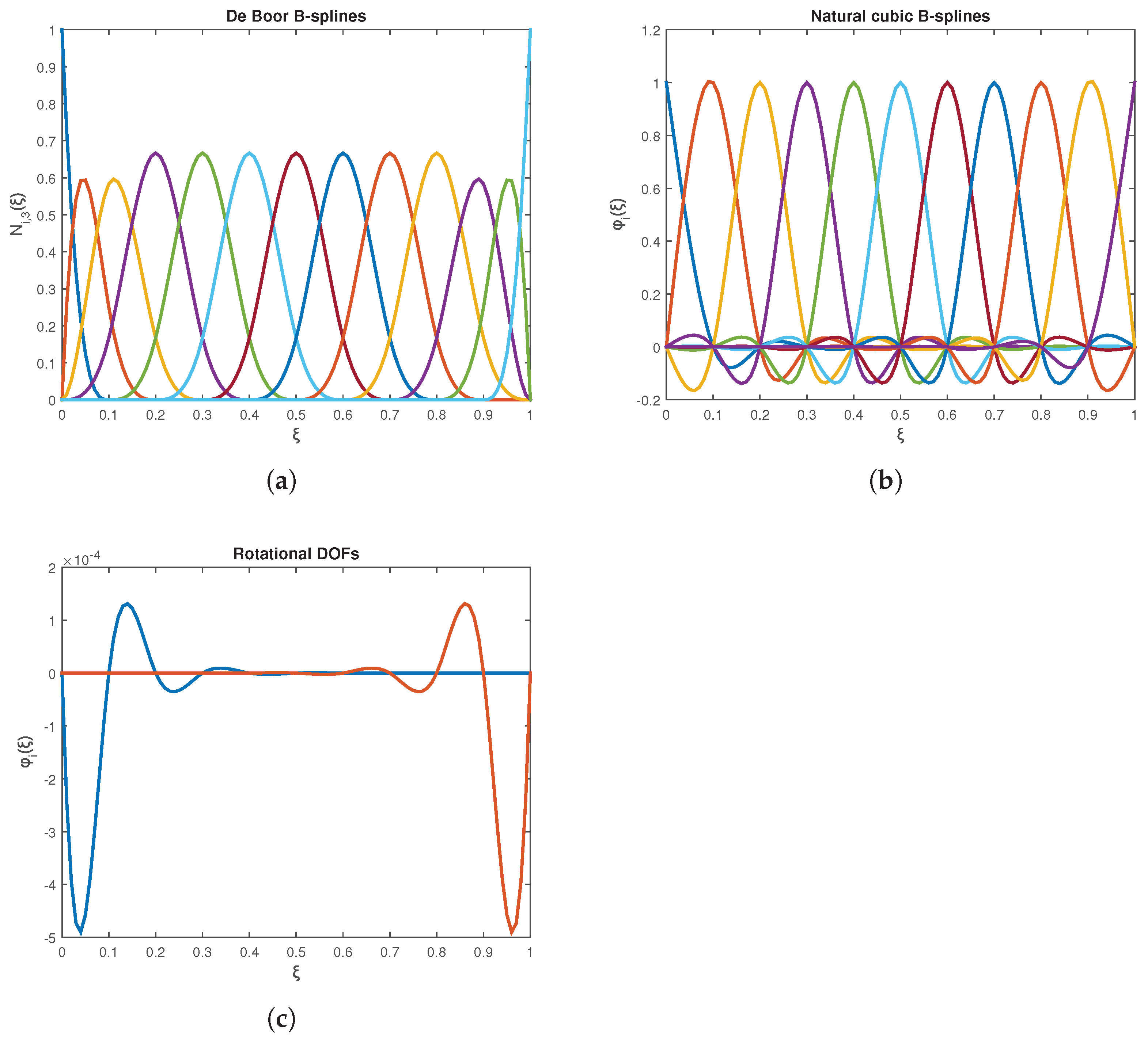
Obviously, the set of de Boor—more precisely, Curry-Schoenberg (1966) [29]—cubic B-splines depicted in Figure A1a is equivalent to the complete set of natural cubic B-splines shown in Figure A1b, augmented by the two basis functions associated with the boundary curvatures illustrated in Figure A1c. This equivalence highlights a critical distinction: earlier analyses that relied solely on natural cubic B-splines, often supplemented by power series expansions (e.g., [2]), inherently lack the full representational capacity of the complete de Boor spline basis. As a result, such approaches may yield solutions of inferior fidelity compared to those constructed using the full set of de Boor B-splines.

Table A1.
Typical MATLAB code for calculating and plotting cubic B-splines and natural B-splines .
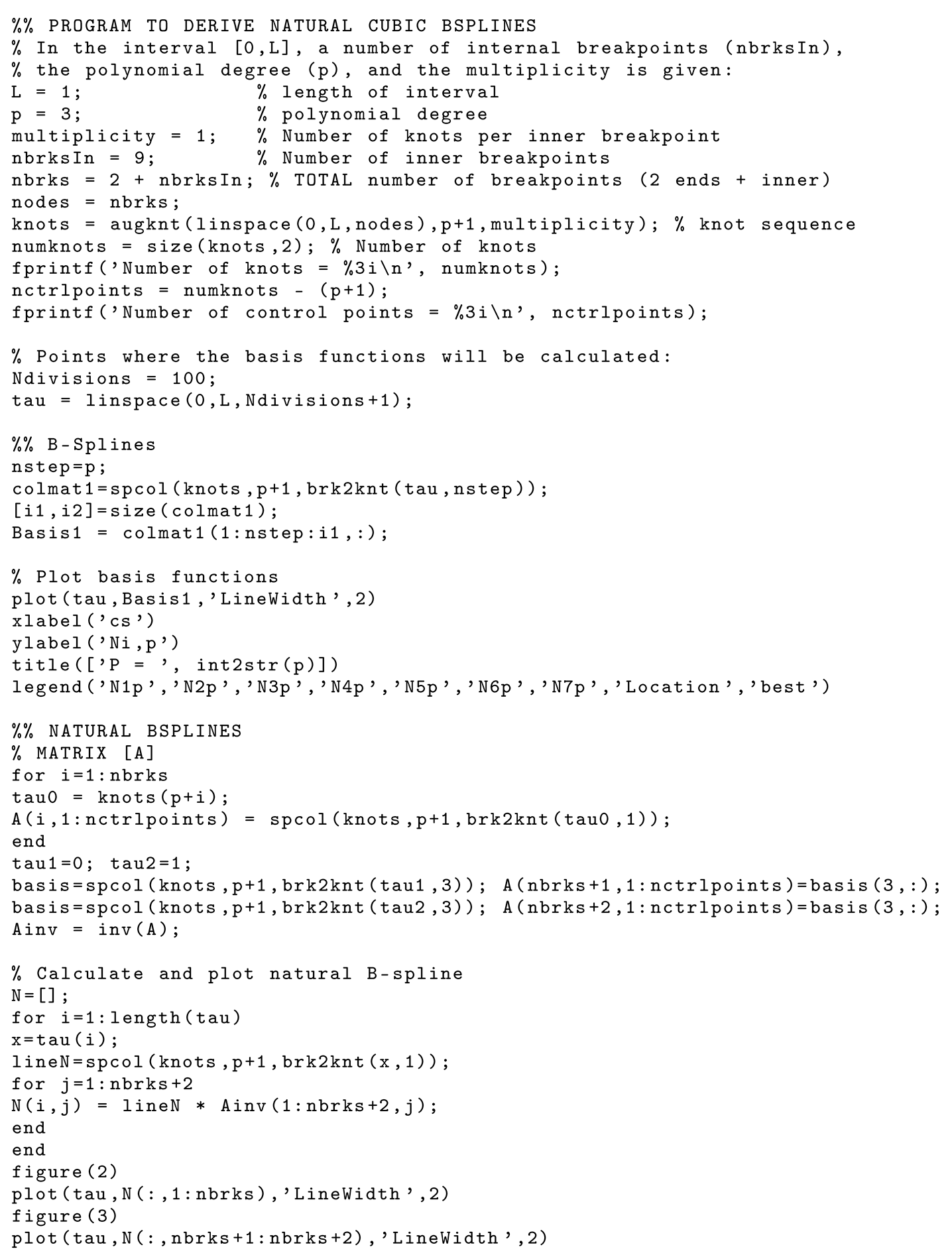
Appendix B. Knot Insertion in One-Dimension
Let us consider the initial knot vector in the interval :
while let the associated control points be
with
In general, if we insert a knot at point with , the updated control points will be given by the linear relationship:
where
Equation (A13) means that the control points remain as are, and thus . Then, p new control points (i.e., ) are introduced according to Equation (A12). At the end, the control points remain as are, and thus .
Applying Equation (A12) successively for some times, the linear relationship between the new (Q) and the old (P) control point becomes:
where is the transformation matrix, produced by the successive implementation of Equation (A12).
In the context of IGA, since the basic assumption of isoparametric property is adopted, the relationship between the new () and the old () coefficients will be:
On the other hand, let the initial set of basis functions be
while the new set of basis functions be
with .
Since the shape and the parameterization is the same (Piegl and Tiller [57]), we have
Equation (A19) is of general nature and relates the initial (P) with the final (Q) set of basis functions, for an arbitrary number of knot insertions. The initial set, , is characterized by -continuity. For each knot insertion, the continuity at the knot under consideration reduces by one, and thus for knot multiplicity , the continuity becomes .
Appendix C. Transformation Matrix Along an Edge or an Isoline
Each mesh-line (station) is determined by its local knot vector knots, which is always defined in the parametric space ranging from zero to unity (i.e., or ). Given the initial set of control points , the updated control points and the corresponding transformation matrix —after knot insertion at —are computed according to Equation (A12) through Equation (A14). A MATLAB® implementation of this procedure, valid for any polynomial degree p, is provided in Table A2.
Table A2.
Transformation matrix along an edge or an isoline.
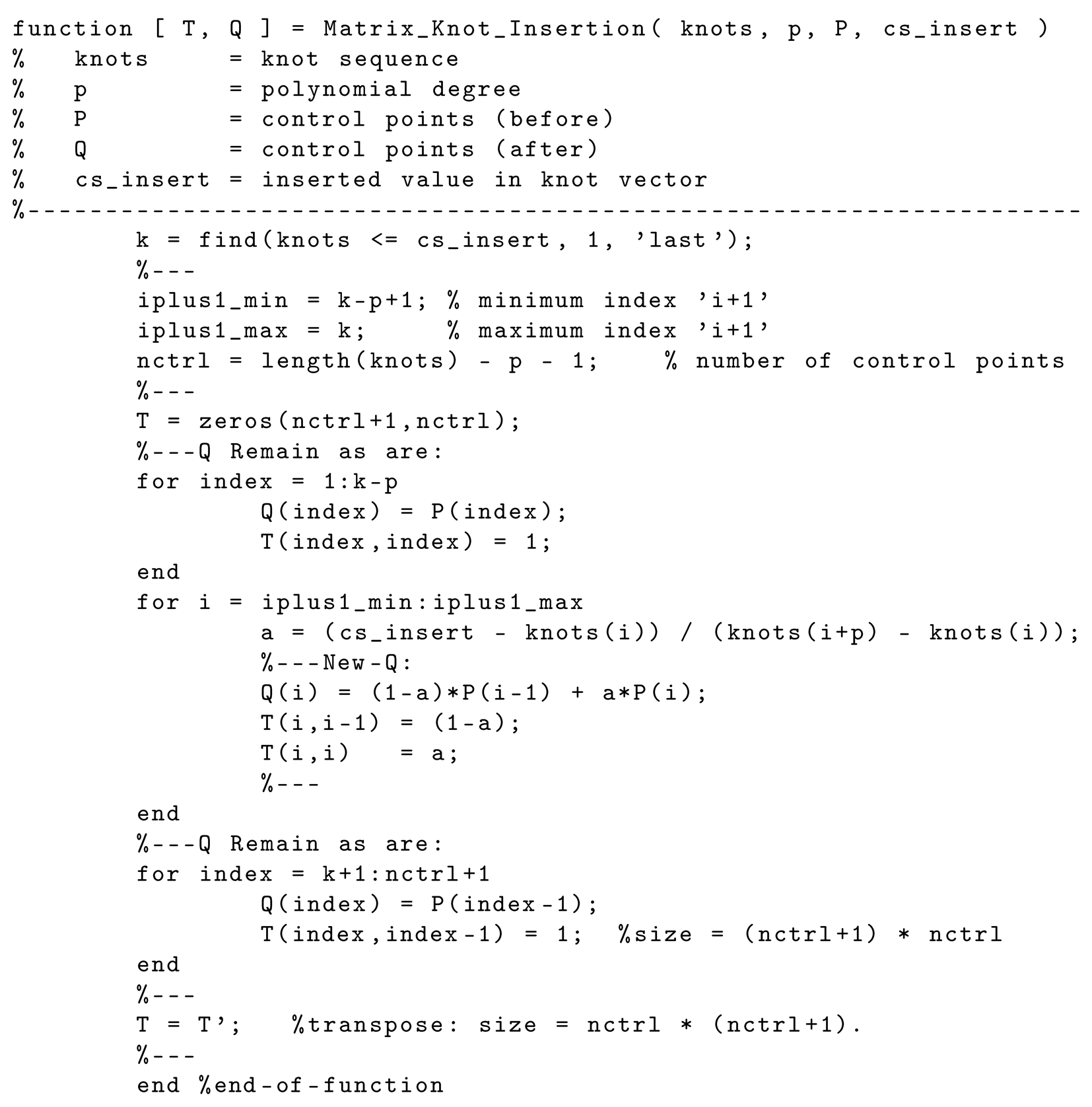
The input to the function Matrix_Knot_Insertion includes the knot vector knots, the polynomial degree p, the control points P, and the insertion value cs_insert corresponding to the parametric coordinate . The function returns the transformation matrix T and the updated control points Q. If only the transformation matrix is required, the input array P may be assigned dummy values (e.g., all entries set to unity), as it does not affect the computation of T.
Numerical application: Considering the incomplete knot vector knot= (i.e., the entry and and are missing), after performing two successive calls of the function Matrix_Knot_Insertion, in which we insert the knots at and , consecutively, the resulting transformation matrix (of size ) is found to be:
One may observe that the sum of the entries of each column in matrix equals unity, which means that the partition of unity property is fulfilled.
Appendix D. Symbolic Derivation of Basis Functions
All the constraints produced by knot insertion are manually introduced in the following MATLAB script, given in Table A3:
Table A3.
Symbolic determination of T-spline basis functions.
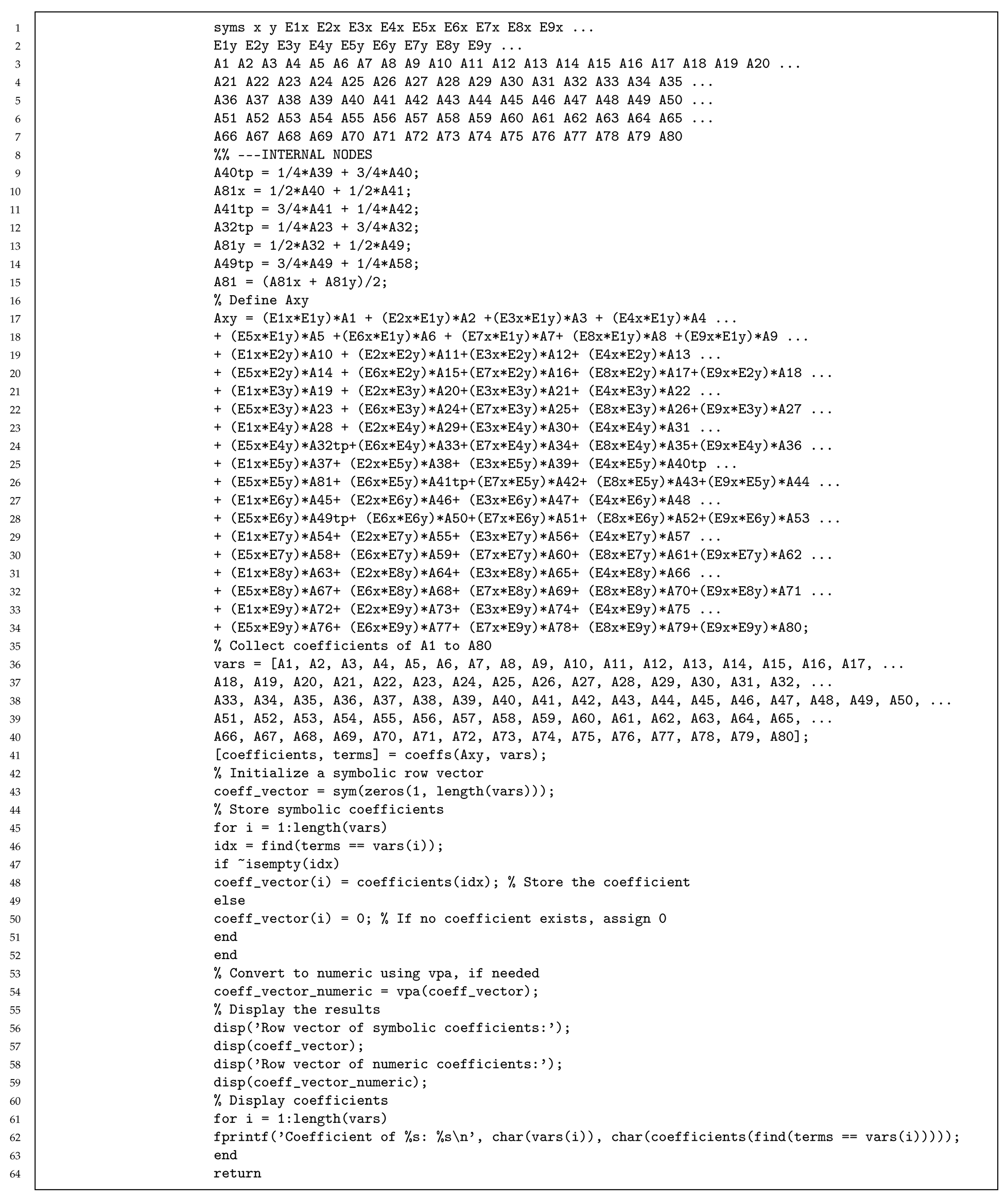
Appendix E. Bernstein Polynomials and Derivatives
It is well known that Bézier interpolation of a curve or a univariate function has the following form
with the Bernstein polynomials given by
whereas are the control points. In case of a univariate function , the control points are substituted by the generalized coefficients , as follows:
To avoid the computation of factorials of Equation (A22) involved in Equation (A21), the values and the first derivative can be alternatively determined using the B-spline technique. The complete in-house function Bernstein is shown in Table A4. It automatically generates the knot vector knots associated with the interval , sets the ends with multiplicity , calls the MATLAB built-in function spcol, and finally stores all the values of into the array Basis, and all the derivatives in array dBasis. These two arrays refer to all sites of vector tau (e.g., at Gauss points). The input variable p is equivalent to the polynomial degree n shown in Eqs. (A21) and (A22).
Table A4.
Computation of Bernstein polynomials and derivatives.
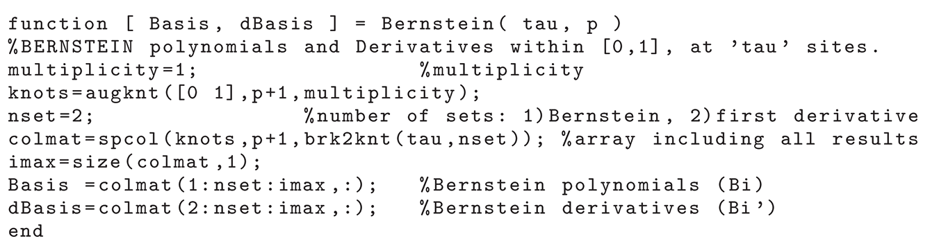
Appendix F. Shape Functions of 12-Node Element
When Bernstein polynomials are used, the bivariate basis functions of the 12-node transfinite element of three layers are given by Equation (20). The MATLAB script, which exits the shape functions, the partial derivatives and the determinant of the Jaxobian matrix at the Gauss points is given below:
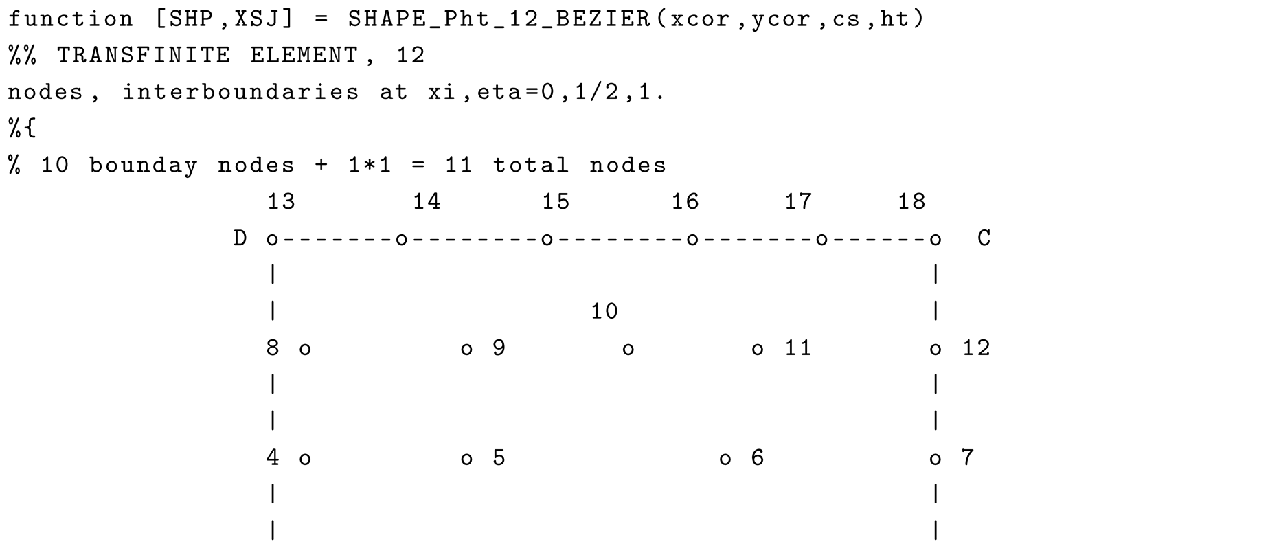
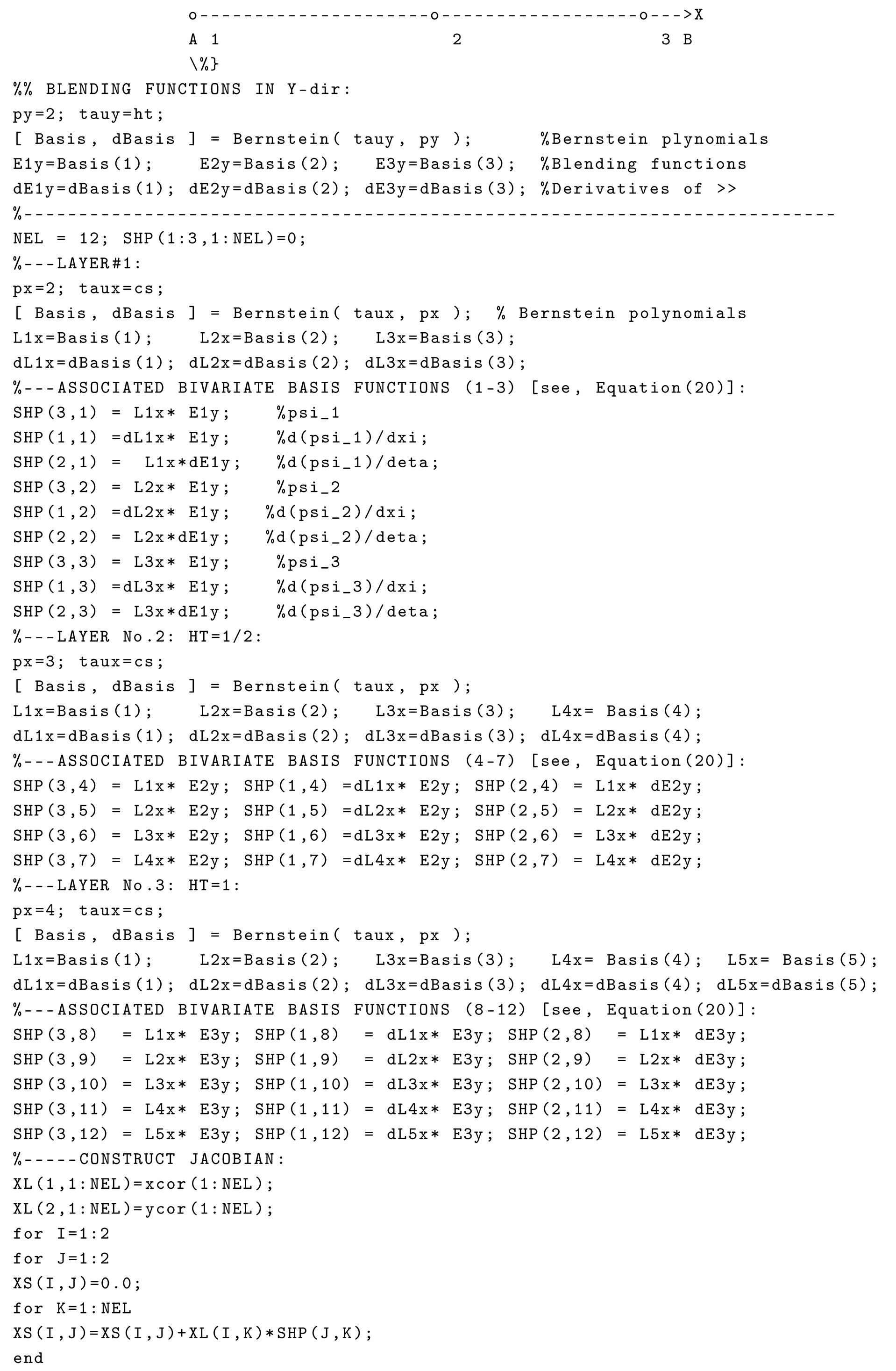
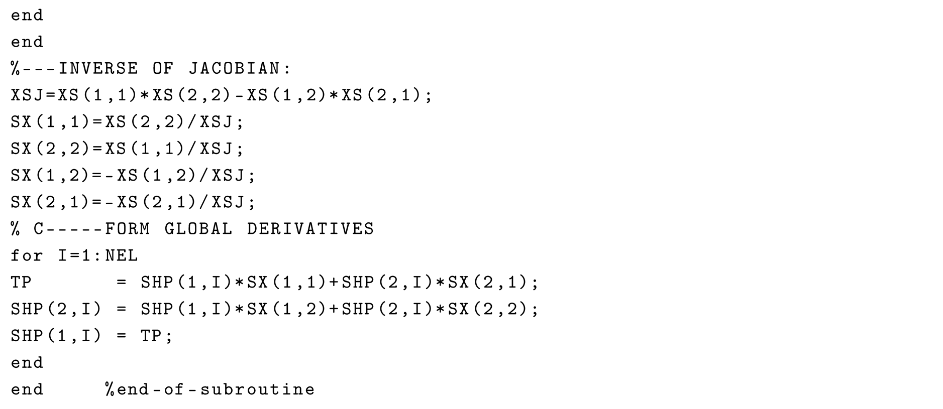
Appendix G. Main Program
Below is the main program for the solution of Example-1 (Figure 16) using the 12-node transfinite element shown in Figure 5a. It calls the four following subroutines,
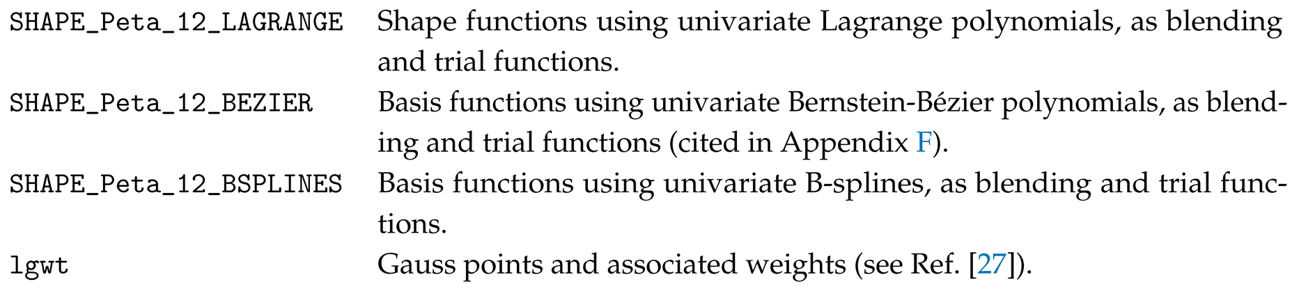
The main integer variables and several real arrays used by the program, together with their meaning are given below.
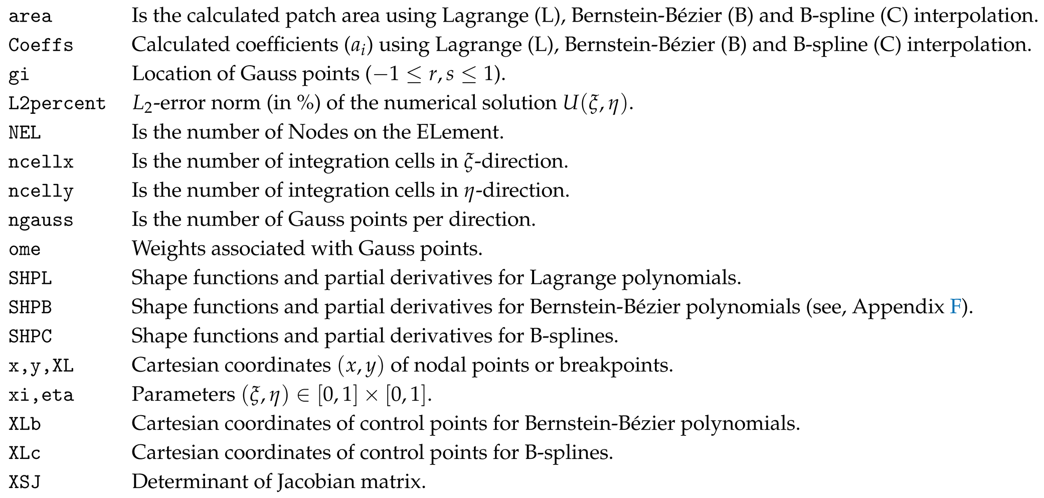
To solve a different problem with a more complex mesh, a preprocessor has to be added with the purpose of replacing the variables x,y at the beginning of the main program.

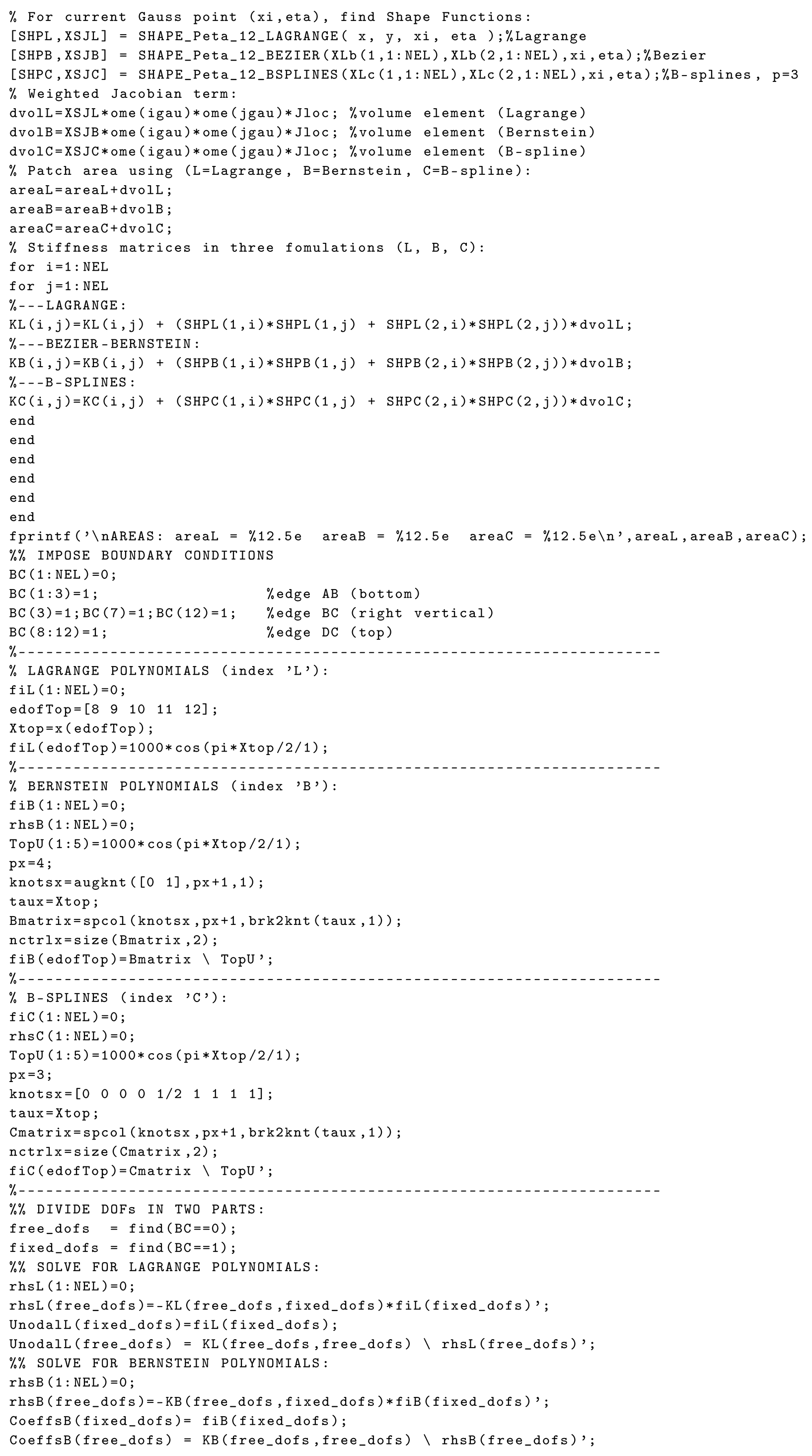
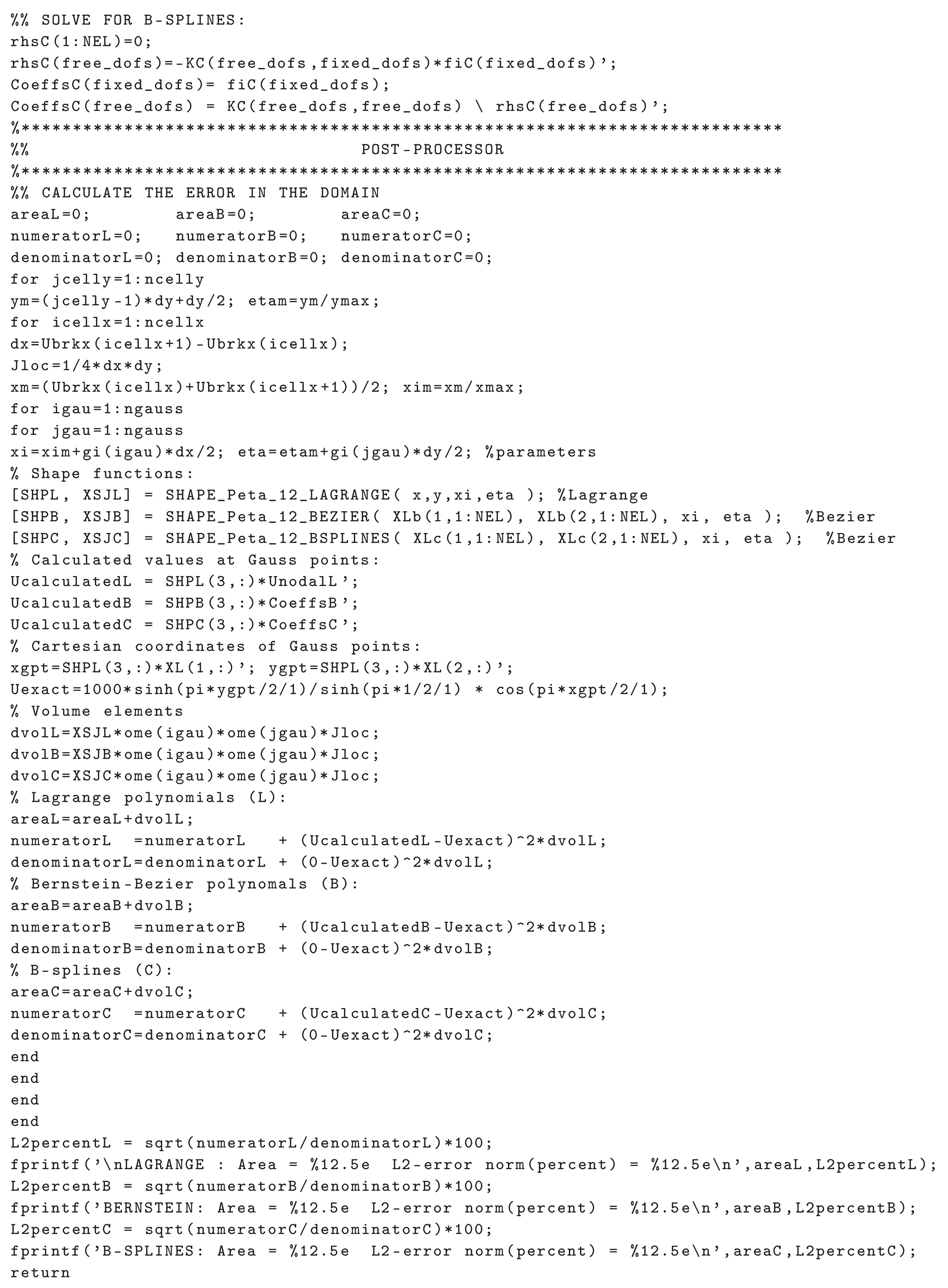
References
- Rayleigh, L. Scientific Papers, Vol. II, Cambridge University Press, Cambridge, 1900.
- Ritz, W. Über eine neue Methode zur Lösung gewisser Variationsprobleme der mathematischen Physik, (On a new method for the solution of certain variational problems of mathematical physics). Journal für reine und angewandte Mathematik 1909;135:1–61.
- Zienkiewicz, OC. The Finite Element Method, 3rd ed. London: McGraw-Hill; 1977.
- Bathe, KJ. Finite Element Procedures, 2nd ed. New Jersey: Prentice-Hall; 1996.
- Gordon WJ, Hall CA. Transfinite element methods: Blending-function interpolation over arbitrary curved element domains. Numerische Mathematik 1973;21:109–129. [CrossRef]
- Birkhoff, G; Cavendish, J.C.; Gordon, W.J. Multivariate Approximation by Locally Blended Univariate Interpolants. Proc. Nat. Acad. Sci. USA 1974;71(9):3423–3425. [CrossRef]
- Coons, SA. Surfaces for computer-aided design of space forms. MIT ( 1967.
- Kanarachos A, Deriziotis D. On the solution of Laplace and wave propagation problems using “C-elements”. Finite elements in Analysis and Design 1989;5(2):97–109. [CrossRef]
- Provatidis, C.G. Precursors of isogeometric analysis: Finite elements, Boundary elements, and Collocation methods. Springer, Cham, 2019. [CrossRef]
- Cottrell JA, Hughes TJR, Bazilevs Y. Isogeometric analysis: towards integration of CAD and FEA, Wiley, Chichester, 2009.
- Scholz E, Altenbach J, Kompatible übergangselemente für lokale Netzverfeinerungen bei 2D- und 3D-Finite-Elemente-Modellen. Tech. Mech. 1985;6:72–78.
- Altenbach J, Scholz E. Ableitung von Formfunktionen für finite Standard- und Übergangselemente Grundlage der gemischten Interpolation. Tech. Mech. 1987;8:18–30.
- Weinberg K, Gabbert U. Adaptive local-global analysis by pNh transition elements. Tech. Mech. 1999;19:115–126.
- Weinberg K, Gabbert U. An adaptive pNh-technique for global-local finite element analysis. Eng. Comput. 2002;19:485–500. [CrossRef]
- Duczek S, Saputra AA, Gravenkamp H. High Order Transition Elements: The xNy-Element Concept–Part I: Statics. Comput. Methods Appl. Mech. Eng. 2020;362:112833. [CrossRef]
- Provatidis, C. Transfinite patches for isogeometric analysis. Mathematics 2025;13(3):35. [CrossRef]
- Sederberg, T.W.; Zheng, J.; Bakenov, A.; Nasri, A. T-splines and T-NURCCs. ACM transactions on graphics (TOG) 2003;22(3):477–484. [CrossRef]
- Bazilevs, Y.; Calo, V.M.; Cottrell, J.A.; Evans, J.A.; Hughes, T.J.R.; Lipton, S.; Scott, M.A.; Sederberg, T.W. Isogeometric analysis using T-splines. Computer Methods in Applied Mechanics and Engineering 2010;199(5–8):229–263. [CrossRef]
- Dörfel, M.R.; Jüttler, B.; Simeon, B. Adaptive isogeometric analysis by local h-refinement with T-splines. Computer Methods in Applied Mechanics and Engineering 2010;199(5–8):264-275. [CrossRef]
- Provatidis, C. Transfinite elements using Bernstein polynomials. Axioms 2025;14(6):433. [CrossRef]
- Provatidis C, Eisenträger S. Macroelement analysis in T-patches using Lagrange polynomials. Mathematics 2025;13(9):1498. [CrossRef]
- Farin, G. Curves and Surfaces for CAGD. Morgan Kaufmann-Elsevier. USA, 2002. [CrossRef]
- Provatidis, C. Bézier versus Lagrange polynomials-based finite element analysis of 2-D potential problems. Advances in Engineering Software 2014;73:22–34. [CrossRef]
- Farouki, R. , and Hinds, J. A hierarchy of geometric forms. IEEE Computer Graphics and Applications 1985;5(5):51–78. [CrossRef]
- Cai Z, Wang W, Du X, Zhao G. A new method for converting trimmed NURBS surface to T-spline surface for isogeometric analysis. AIP Conference Proceedings. Vol. 1834. No. 1. AIP Publishing, 2017. [CrossRef]
- DeBoor C, A Practical Guide to Splines, Revised ed., Springer: New York, 2001.
- Greg von Winckel (2025). Legendre-Gauss Quadrature Weights and Nodes (https://www.mathworks.com/matlabcentral/fileexchange/4540-legendre-gauss-quadrature-weights-and-nodes), MATLAB Central File Exchange. Recovered , 2025. 6 August.
- Carslaw HS, Jaeger JC. Conduction of Heat in Solids. 2nd ed. Oxford: Oxford University Press; 1969.
- Curry HB, Schoenberg IJ. On Pólya Frequency Functions IV: The Fundamental spline functions and their limits. Journal d’Analyse Mathématique 1966;17(1):71–107. [CrossRef]
- Cox, MG. The Numerical Evaluation of B-Splines. IMA Journal of Applied Mathematics 1972;10(2):134–149. [CrossRef]
- De Boor, C. On Calculating with B-Splines. Journal of Approximation Theory 1972;6(1):50–62. [CrossRef]
- Karniadakis GE, Sherwin SJ. Spectral/ Hp Element Methods for Computational Fluid Dynamics. Oxford: Oxford Science Publications; 2005. [CrossRef]
- Courant R, Hilbert D. Methods of mathematical physics (1st English ed., Vol. I). New York: InterScience (translated and revised from the German original); 1966.
- Felippa CA, Haugen B, Militello C. From the individual element test to finite element templates: Evolution of the patch test. International Journal for Numerical Methods in Engineering 1995:38(2):199–229. [CrossRef]
- Provatidis, CG. , Lumped mass acoustic and membrane eigenanalysis using the global collocation method. Cogent Engineering 2014;1(1), Article: 981366. [CrossRef]
- Provatidis CG, CAD-based collocation eigenanalysis of 2-D elastic structures, Computers and Structures 2017,182:55–73. [CrossRef]
- Yağmurlu NM, Karakaş AS, A novel perspective for simulations of the MEW equation by trigonometric cubic B-spline collocation method based on Rubin-Graves type linearization. Computational Methods for Differential Equations 2022;10(4):1046–1058. [CrossRef]
- Kutluay S, Yağmurlu NM, Karakaş AS, A novel perspective for simulations of the Modified Equal-Width Wave equation by cubic Hermite B-spline collocation method. Wave Motion 2024;129:103342. [CrossRef]
- Kutluay S, Yagmurlu NM, Karakaş AS, A robust septic hermite collocation technique for dirichlet boundary condition Heat conduction equation. International Journal of Mathematics and Computer in Engineering 2025;3(2):253–266.
- Eisenträger S, Eisenträger J, Gravenkamp H, Provatidis CG. High order transition elements: The xNy-element concept, Part II: Dynamics. Computer Methods in Applied Mechanics and Engineering 2021;387:114145. [CrossRef]
- Provatidis C, Sevilla R, Schillinger D, Eisenträger S. Revisiting Transfinite Elements: Unifying Element Formulations for IGA, SEM, NEFEM, p-FEM and h-FEM. Archives of Computational Methods in Engineering 2025 (in press). [CrossRef]
- Provatidis, CG. Non-rational and rational transfinite interpolation using Bernstein polynomials. International Journal of Computational Geometry and Applications 2022;32(1-2):55–89. [CrossRef]
- Zepeng Wen, Qiong Pan, Xiaoya Zhai, Hongmei Kang, Falai Chen, Adaptive isogeometric topology optimization of shell structures based on PHT-splines, Computers & Structures 2024;305:107565. [CrossRef]
- Chenk K, Qiu C, Liu Z, Tan J. A high-precision T-spline blade modeling method with 2D and 3D knot adaptive refinement. Advances in Engineering Software 2024;194:103684. [CrossRef]
- Nguyen VP, Anitescu C, Bordas SP, Rabczuk T. Isogeometric analysis: an overview and computer implementation aspects. Mathematics and Computers in Simulation 2015;117:89-116. [CrossRef]
- Garau EM, Vázquez R. Algorithms for the implementation of adaptive isogeometric methods using hierarchical B-splines. Applied Numerical Mathematics 2018;123:58-87. [CrossRef]
- Provatidis CG, Angelidis DI. Performance of Coons’ macroelements in plate bending analysis. International Journal for Computational Methods in Engineering Science and Mechanics 2014;15(2):110–125. [CrossRef]
- Bogner FK, Fox RL, Schmit LA. The generation of inter-element-compatible stiffness and mass matrices by the use of interpolation formulas. In Proceedings of the Conference on Matrix Methods in Structural Mechanics (1965), pp. 397–444.
- Thomas DC, Engvall L, Schmidt SK, Tew K, Scott MA. U-splines: Splines over unstructured meshes. Computer Methods in Applied Mechanics and Engineering 2022;401:115515. [CrossRef]
- Wei X, Li X, Qian K, Hughes TJR, Zhang YJ, Casquero H. Analysis-suitable unstructured T-splines: Multiple extraordinary points per face. Computer Methods in Applied Mechanics and Engineering 2022;391:114494. [CrossRef]
- Sangalli G, Takacs T, Vázquez R. Unstructured spline spaces for isogeometric analysis based on spline manifolds. Computer Aided Geometric Design 2016;47:61–82.
- Banh, TT, Lieu QX, Kang J, Ju Y, Shin S, Lee D. A novel robust stress-based multimaterial topology optimization model for structural stability framework using refined adaptive continuation method. Engineering with Computers 2024;40(2):677–713. [CrossRef]
- Nguyen MN, Lee D. Design of the multiphase material structures with mass, stiffness, stress, and dynamic criteria via a modified ordered SIMP topology optimization. Advances in Engineering Software 2024;189:103592. [CrossRef]
- Banh TT, Lieu QX, Nguyen SH, Lee D. Stress-driven design of incompressible multi-materials under frequency constraints. International Journal of Mechanical Sciences 2024;277:109416. [CrossRef]
- Nguyen MN, Hoang VN, Lee D. Multiscale topology optimization with stress, buckling and dynamic constraints using adaptive geometric components. Thin-Walled Structures 2023;183:111405. [CrossRef]
- Banh TT, Lee D. Comprehensive polygonal topology optimization for triplet thermo-mechanical-pressure multi-material systems. Engineering with Computers 2024;40(5):3295–3317. [CrossRef]
- Piegl L, Tiller W. The NURBS Book, 2nd ed. Berlin; New York: Springer; 1997. ISBN: 978-3-642-59223-2. https://link.springer.com/book/10. 1007.
- Farin, G. Curves and Surfaces for CAGD: A Practical Guide, 5th ed. Morgan Kaufmann: San Francisco, USA, 2002.
- Piegl, L; Tiller, W. The NURBS Book, 2nd ed. Springer: Berlin, Germany, 1997.
- Hoschek, J.; Lasser, D. Fundamentals of computer aided geometric design, 2nd ed. A.K. Peters: Wellesley, Mass, 1996.
- Hughes, T. J. R.; Cottrell, J. A.; Bazilevs, Y. (2005). Isogeometric analysis: CAD, finite elements, NURBS, exact geometry and mesh refinement. Computer Methods in Applied Mechanics and Engineering, 4135. [Google Scholar] [CrossRef]
- Desiderio, L.; D’Inverno, G.A.; Sampoli, M.L.; Sestini, A. Hierarchical matrices for 3D Helmholtz problems in the multi-patch IgA-BEM setting. Engineering with Computers 2025;41, 2021–2042. [CrossRef]
- Schillinger, D.; Ruthala, P. K.; Nguyen, L. H. Lagrange extraction and projection for NURBS basis functions: A direct link between isogeometric and standard nodal finite element formulations. International Journal for Numerical Methods in Engineering. [CrossRef]
- Liu, B.; Xing, Y.; Wang, Z.; Lu, X.; Sun, H. Non-uniform rational Lagrange functions and its applications to isogeometric analysis of in-plane and flexural vibration of thin plates. Computer Methods in Applied Mechanics and Engineering. [CrossRef]
- Lu, L. Z. Adaptive Polynomial Approximation to Circular Arcs. Applied Mechanics and Materials. [CrossRef]
- Vavpetič, A. Optimal parametric interpolants of circular arcs. Computer Aided Geometric Design, 1018. [Google Scholar] [CrossRef]
- Vavpetič, A.; Žagar, E. A general framework for the optimal approximation of circular arcs by parametric polynomial curves. Journal of Computational and Applied Mathematics. [CrossRef]
- Vavpetič, A.; Žagar, E. On optimal polynomial geometric interpolation of circular arcs according to the Hausdorff distance. Journal of Computational and Applied Mathematics, 1134. [Google Scholar] [CrossRef]
- De Boor, C. A Practical Guide to Splines, rev ed. Applied mathematical sciences. Springer: New York, 2001.
- Patera, A.T. A spectral element method for fluid dynamics: Laminar flow in a channel expansion. Journal of Computational Physics. [CrossRef]
- Pozrikidis, C. Introduction to Finite and Spectral Element Methods Using MATLAB, 2nd ed. CRC Press: Boca-Raton, 2014.
- Eisenträger, S.; Eisenträger, J.; Gravenkamp, H.; Provatidis, C.G. High order transition elements: The xNy-element concept-part II: Dynamics. Computer Methods in Applied Mechanics and Engineering, 2021. [Google Scholar] [CrossRef]
- Provatidis, C.G. Precursors of Isogeometric Analysis: Finite Elements, Boundary Elements, and Collocation Methods. Solid Mechanics and Its Applications. Springer International Publishing: Cham, 2019. [CrossRef]
- Piegl, L.; Tiller, W. A menagerie of rational B-spline circles. IEEE Computer Graphics and Applications. [CrossRef]
- Provatidis, C. How accurately can spherical caps be represented by rational quadratic polynomials? WSEAS Transactions on Computers 2021;20, 139–146. [CrossRef]
- Cobb, J.E. Tiling the Sphere with Rational Bézier Patches, TR UUCS-88-009, 1988. Download from: https://core.ac.uk/download/pdf/276277507.pdf (see also, Letter to the editor, Computer Aided Geometric Design 1989; 6(1)). 6.
- Levenberg, K. A Method for the Solution of Certain Problems in Least-Squares. Quarterly Applied Mathematics. [CrossRef]
- Marquardt, D. An Algorithm for Least-squares Estimation of Nonlinear Parameters. SIAM Journal Applied Mathematics. [CrossRef]
- Carslaw, H.S.; Jaeger, J.C. Conduction of Heat in Solids, 2nd ed. Oxford: Oxford University Press, 1969.
Figure 1.
(a) Coons element. (b) Tensor-product element. (c) Classical transfinite element. (d) Arbitrary-noded boundary with inner tensor-product element. (e) One-directional element.
Figure 1.
(a) Coons element. (b) Tensor-product element. (c) Classical transfinite element. (d) Arbitrary-noded boundary with inner tensor-product element. (e) One-directional element.
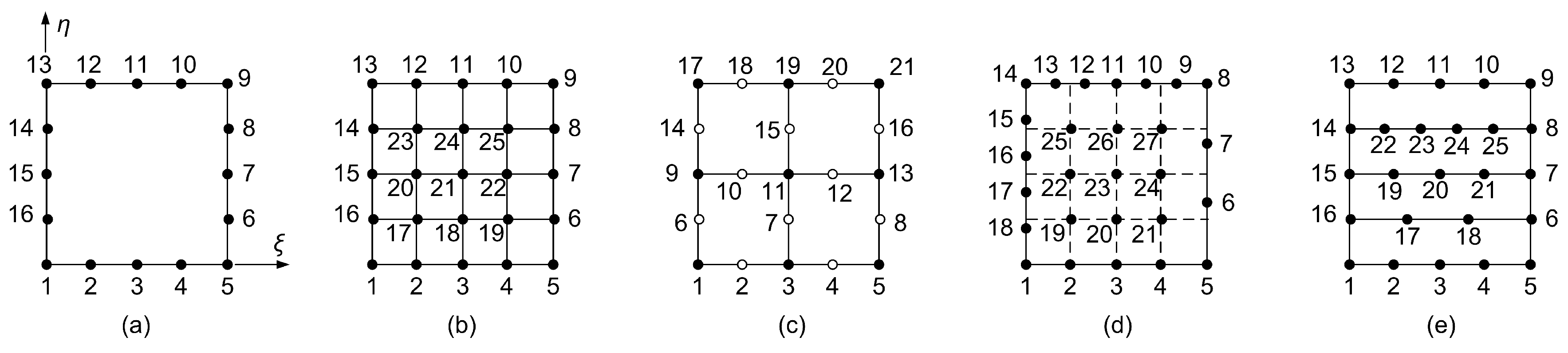
Figure 2.
(a) One-dimensional curve. (b) Two-dimensional patch.
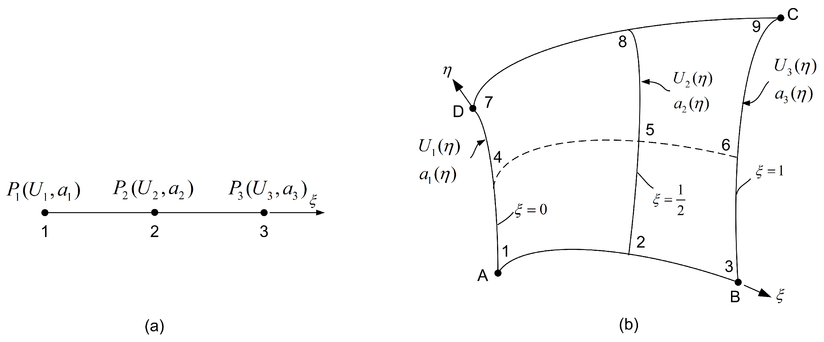
Figure 3.
A collection of classical transfinite elements: (a) 21-node element. (b) 27-node element. (c) 33-node element. (d) 113-node element.
Figure 3.
A collection of classical transfinite elements: (a) 21-node element. (b) 27-node element. (c) 33-node element. (d) 113-node element.
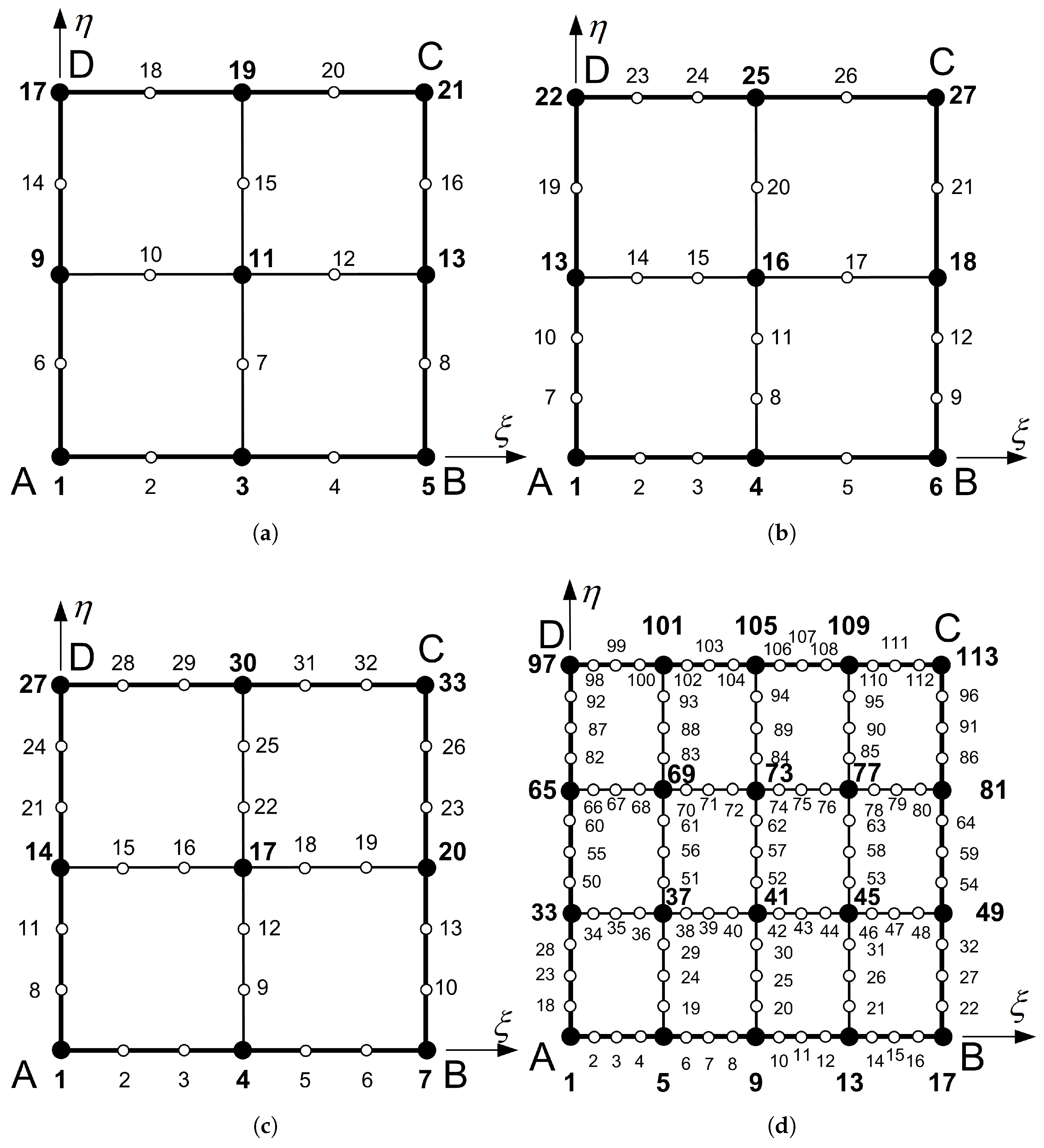
Figure 4.
Bivariate basis functions for the 113-node transfinite element, using Lagrange polynomials as blending functions, while trial functions are: (a) Lagrange polynomials; (b) natural cubic cardinal B-splines; (c) de Boor cubic B-splines.
Figure 4.
Bivariate basis functions for the 113-node transfinite element, using Lagrange polynomials as blending functions, while trial functions are: (a) Lagrange polynomials; (b) natural cubic cardinal B-splines; (c) de Boor cubic B-splines.
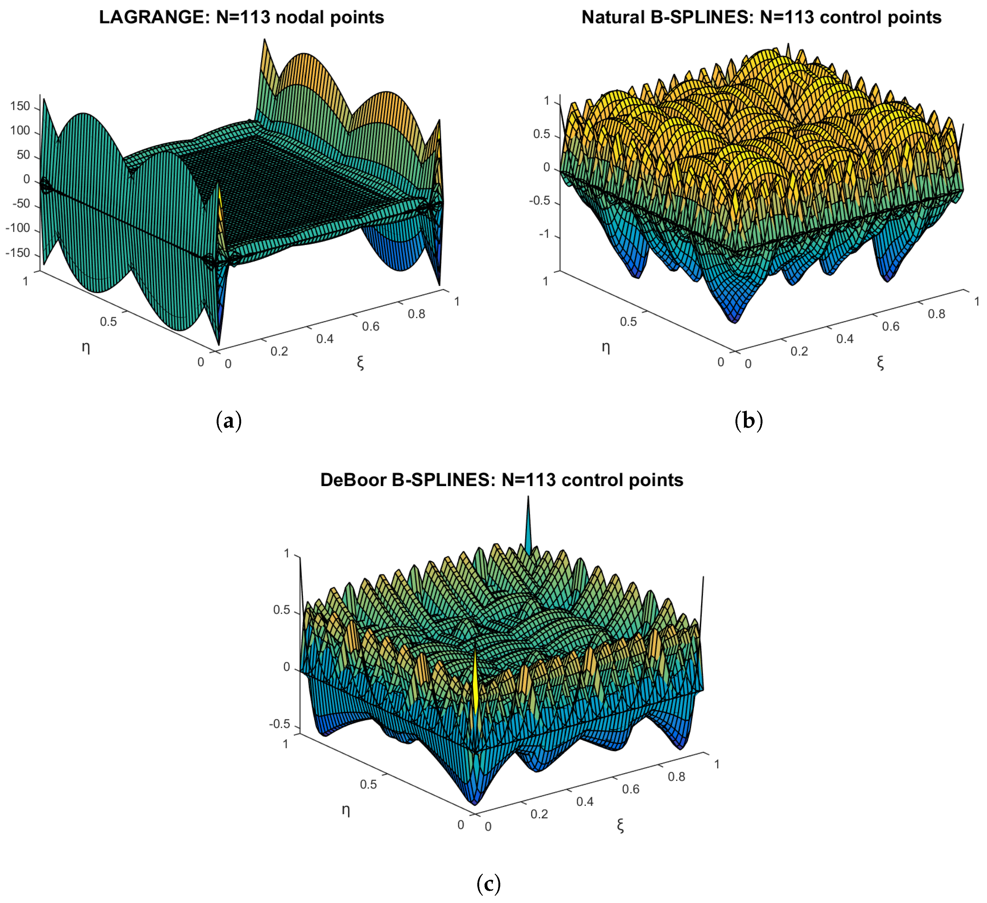
Figure 5.
Transitional elements: (a) 12-node; (b) 18-node; (c) 25-node; (d) 32-node element.
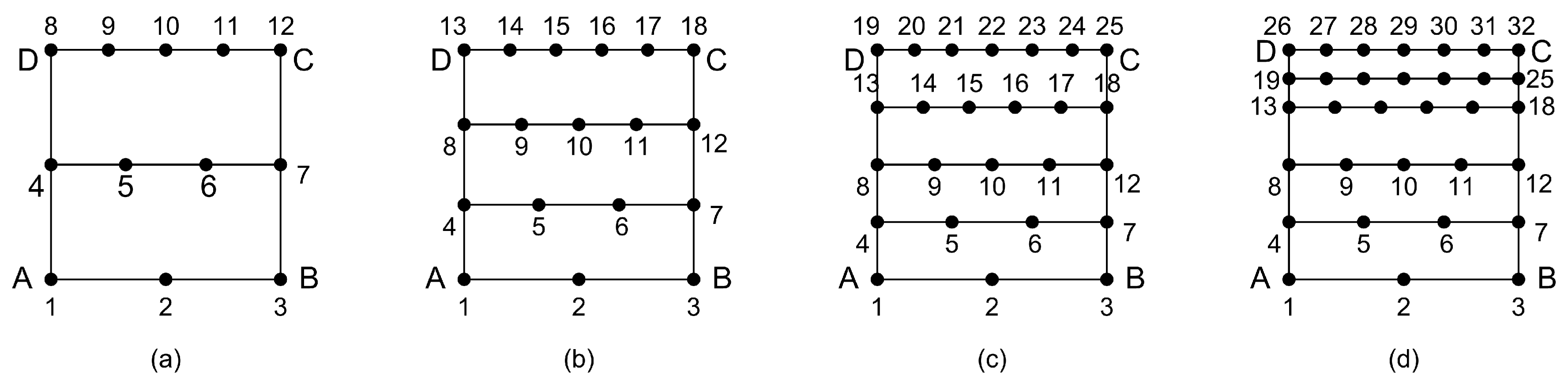
Figure 6.
12-node transition element: (a) Lagrange polynomials; (b) Bernstein polynomials.
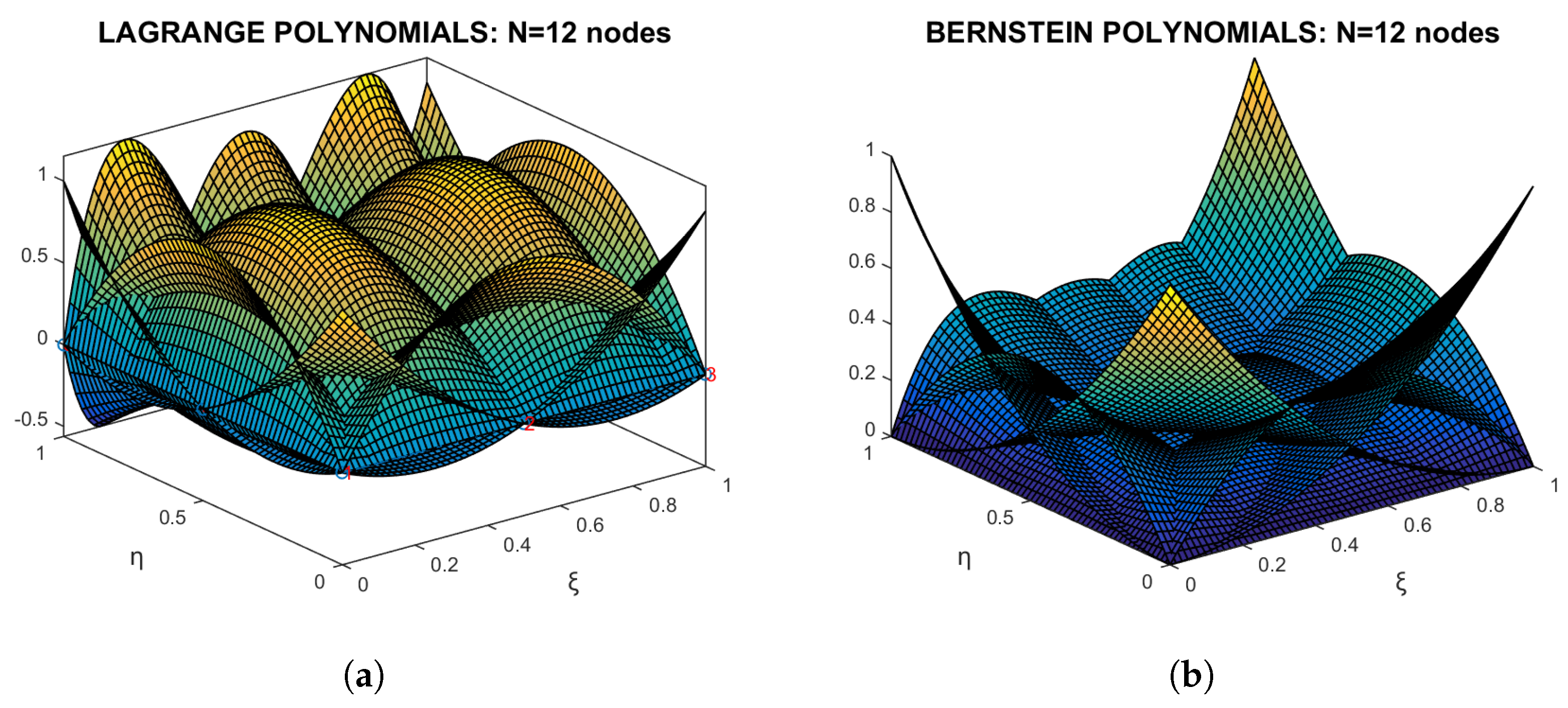
Figure 7.
Basis functions for the 18-node transfinite element: (a) Lagrange polynomials; (b) Bernstein polynomials; (c) Mixed, Bernstein polynomials and B-splines.
Figure 7.
Basis functions for the 18-node transfinite element: (a) Lagrange polynomials; (b) Bernstein polynomials; (c) Mixed, Bernstein polynomials and B-splines.
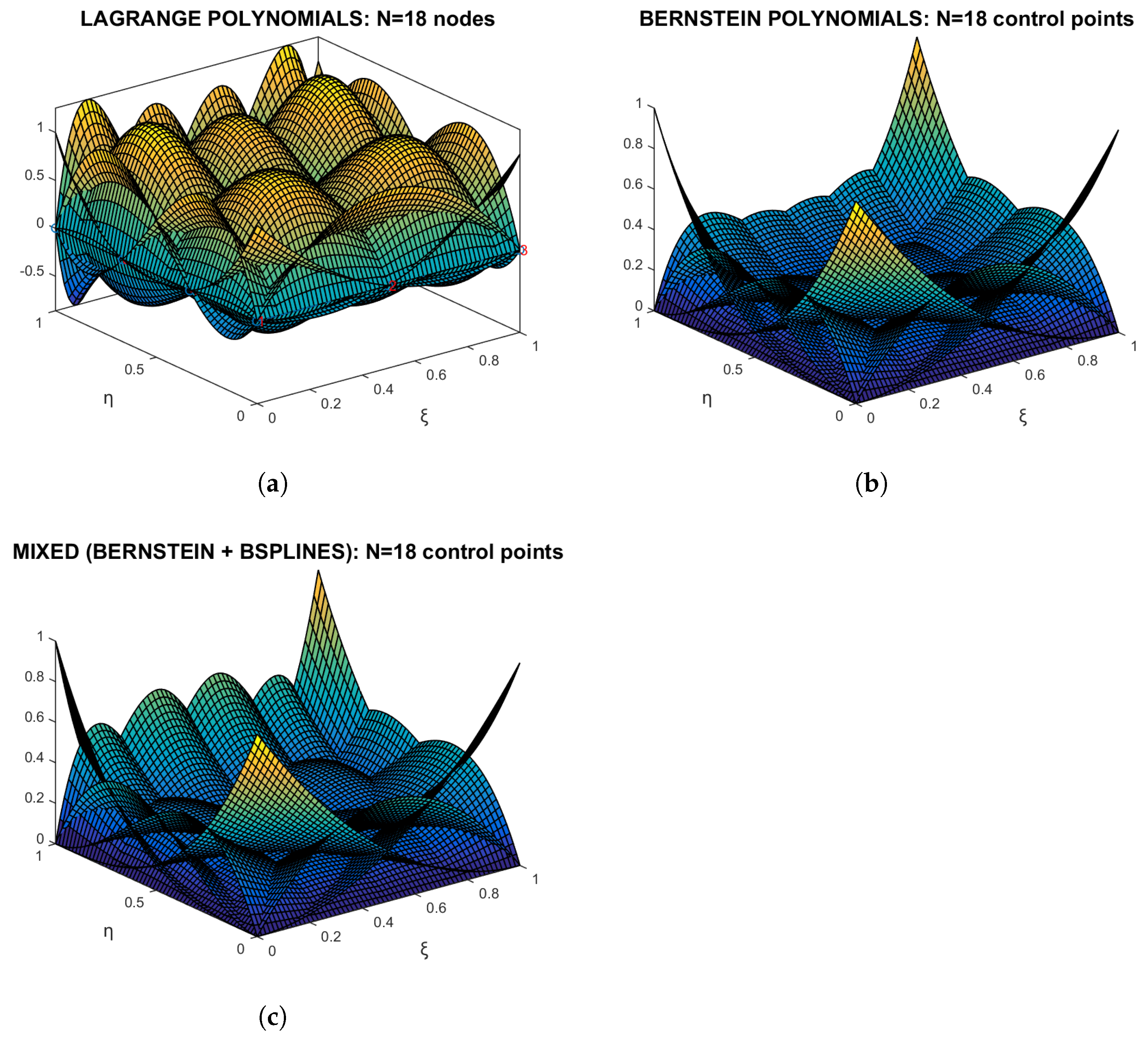
Figure 8.
27-node transfinite element.
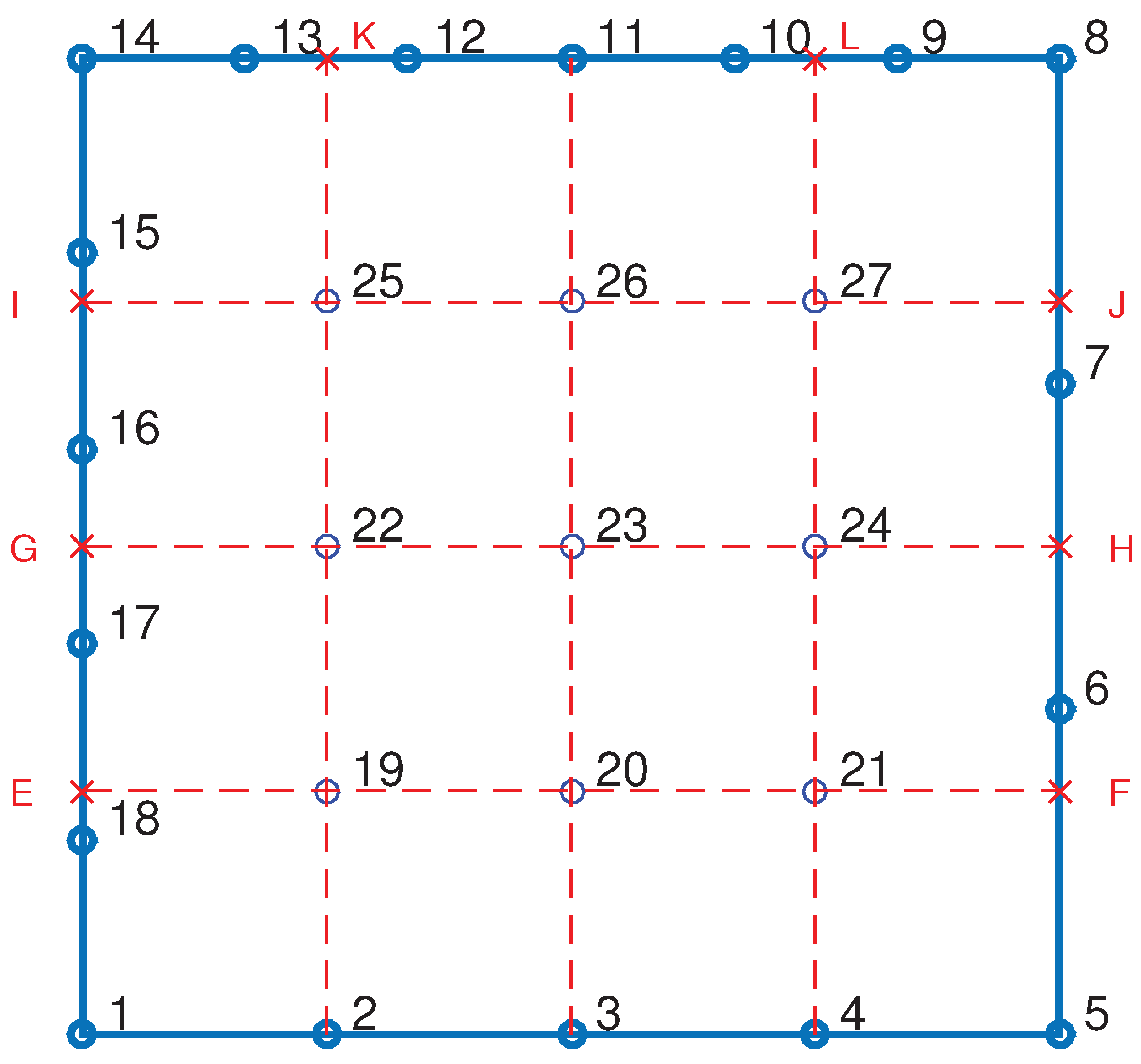
Figure 9.
27-DOF B-spline transfinite element.
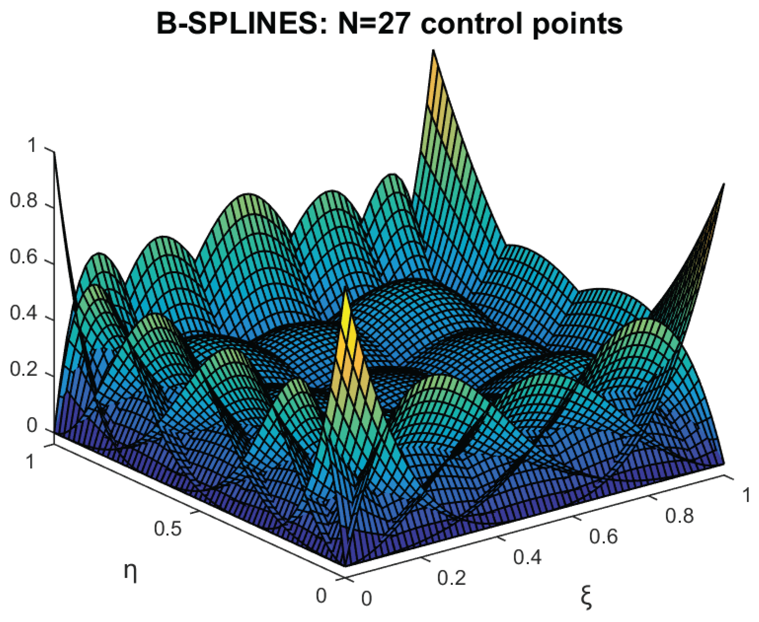
Figure 10.
T-spline transfinite elements: (a) Tensor-product 81-node; (b) 76-node; (c) 73-node element. Missing nodes in tensor product are denoted by a skew red cross (×).
Figure 10.
T-spline transfinite elements: (a) Tensor-product 81-node; (b) 76-node; (c) 73-node element. Missing nodes in tensor product are denoted by a skew red cross (×).
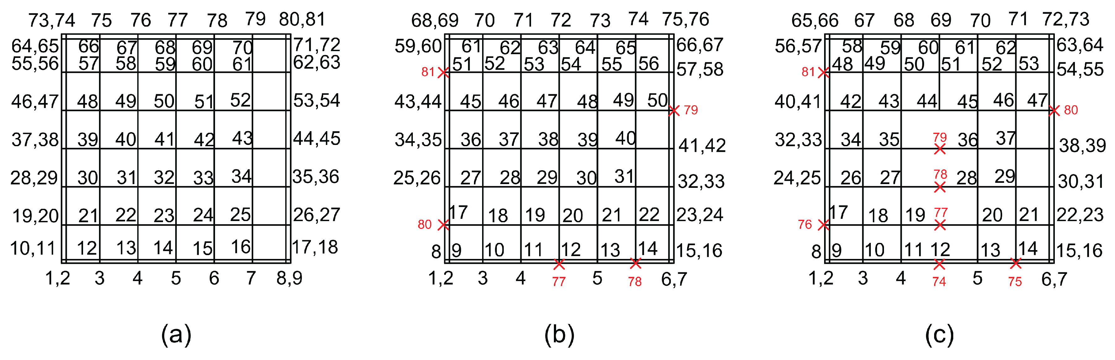
Figure 11.
B-splines along the bottom edge .
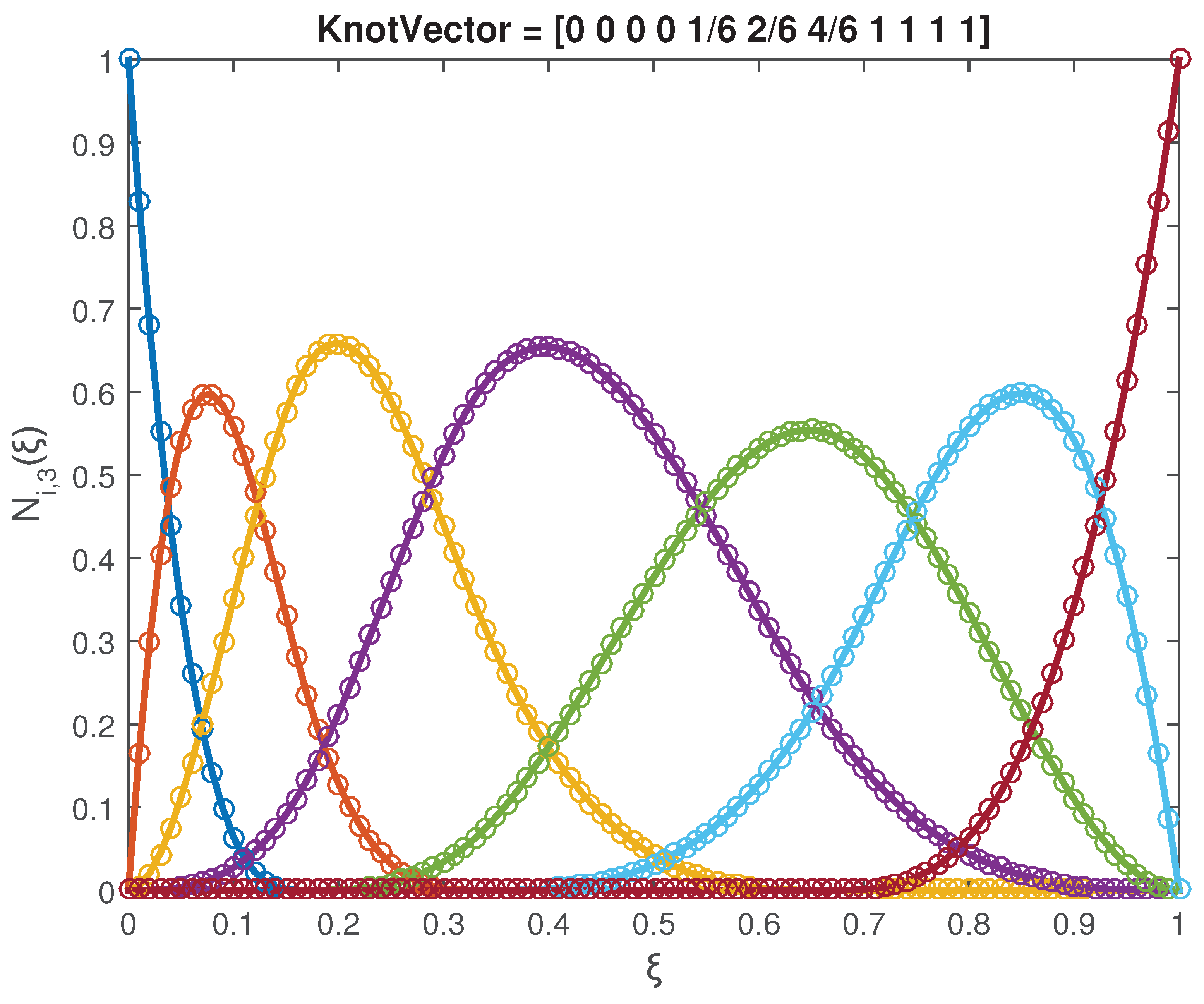
Figure 12.
76-node T-spline transfinite element with affected boundary.
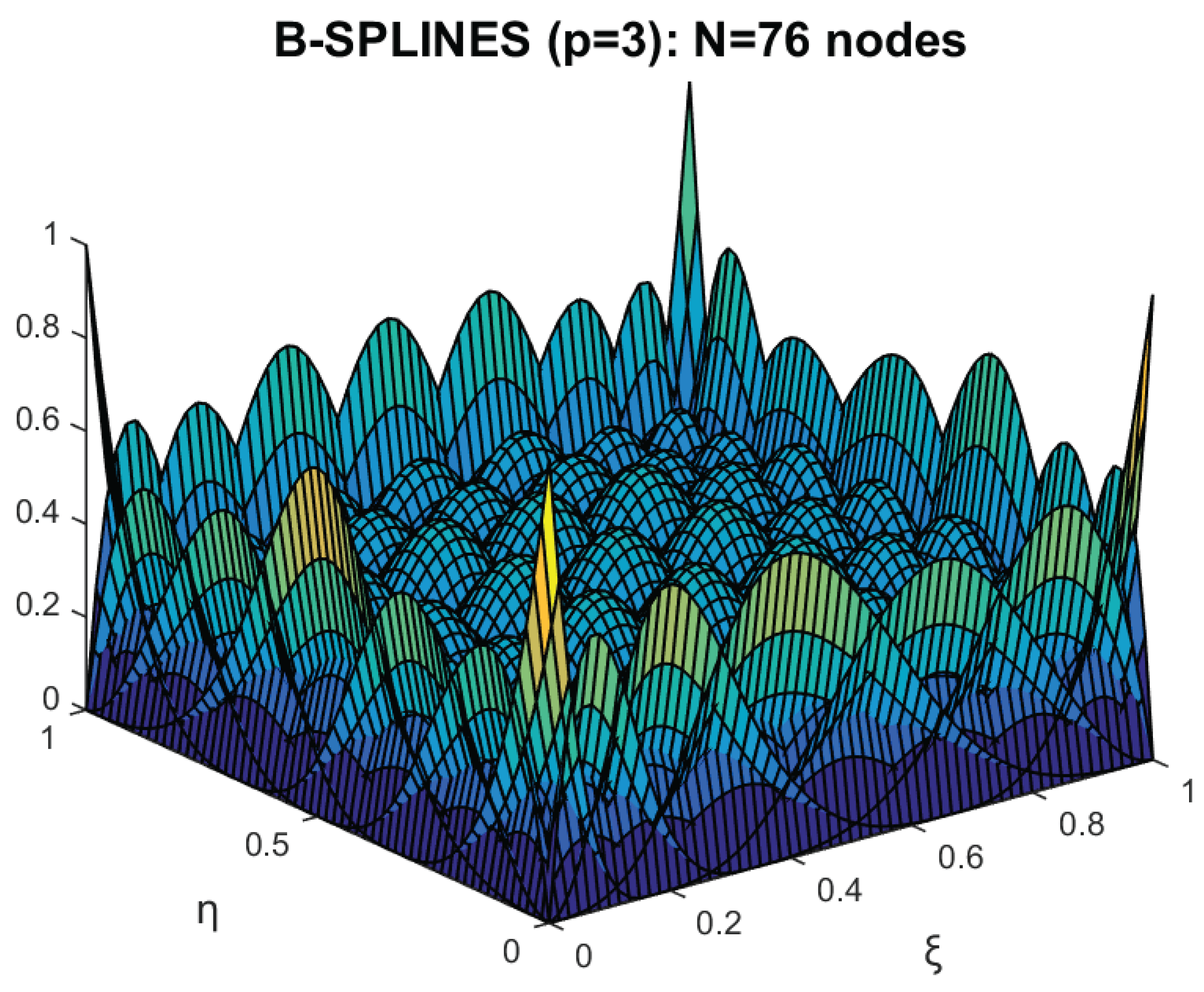
Figure 13.
73-node T-spline transfinite element with affected boundary plus three internal nodes.
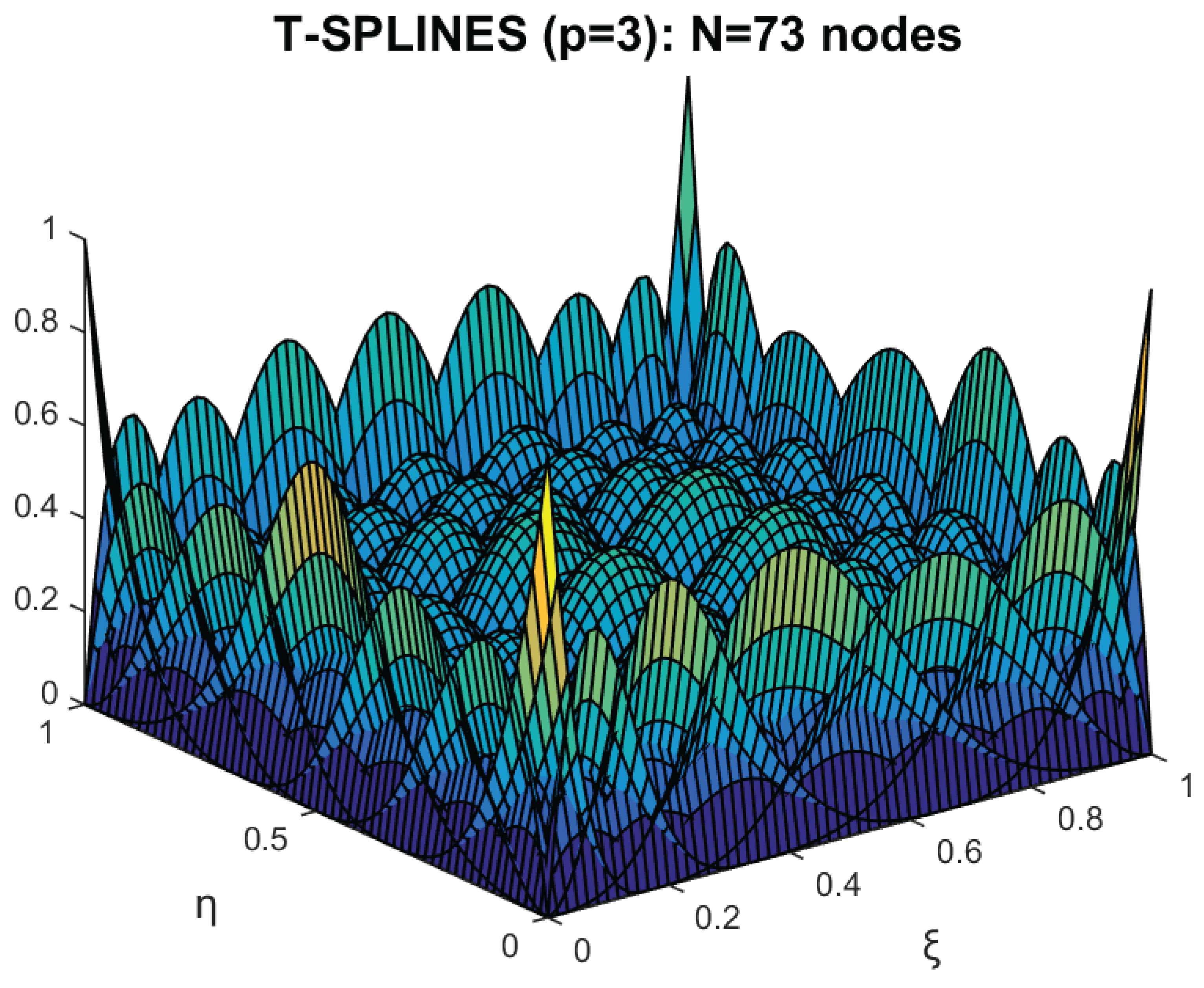
Figure 14.
Missing central node in an 80-node transfinite element.
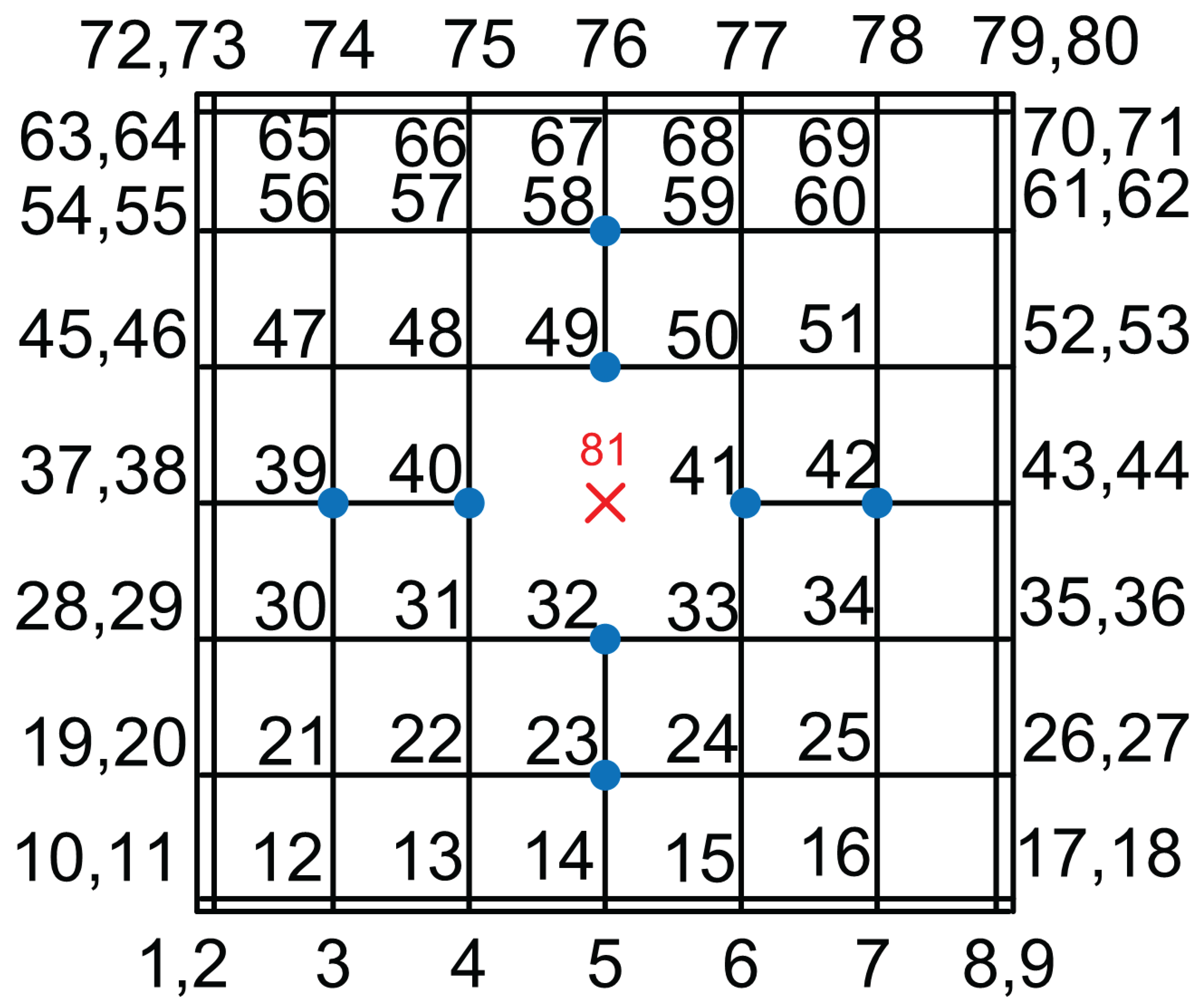
Figure 15.
80-node T-spline transfinite element with missing central vertex.
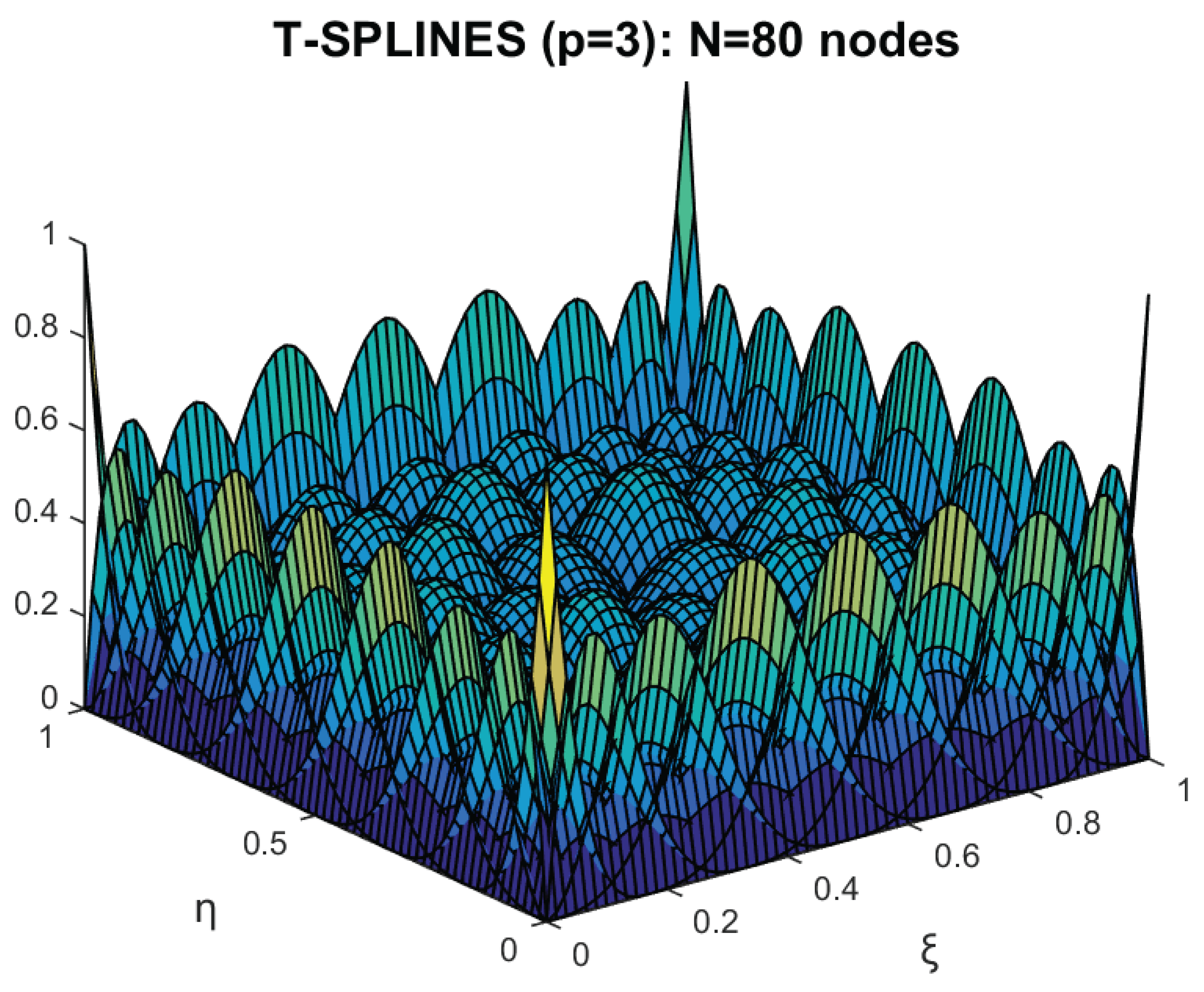
Figure 16.
Geometry and boundary conditions.
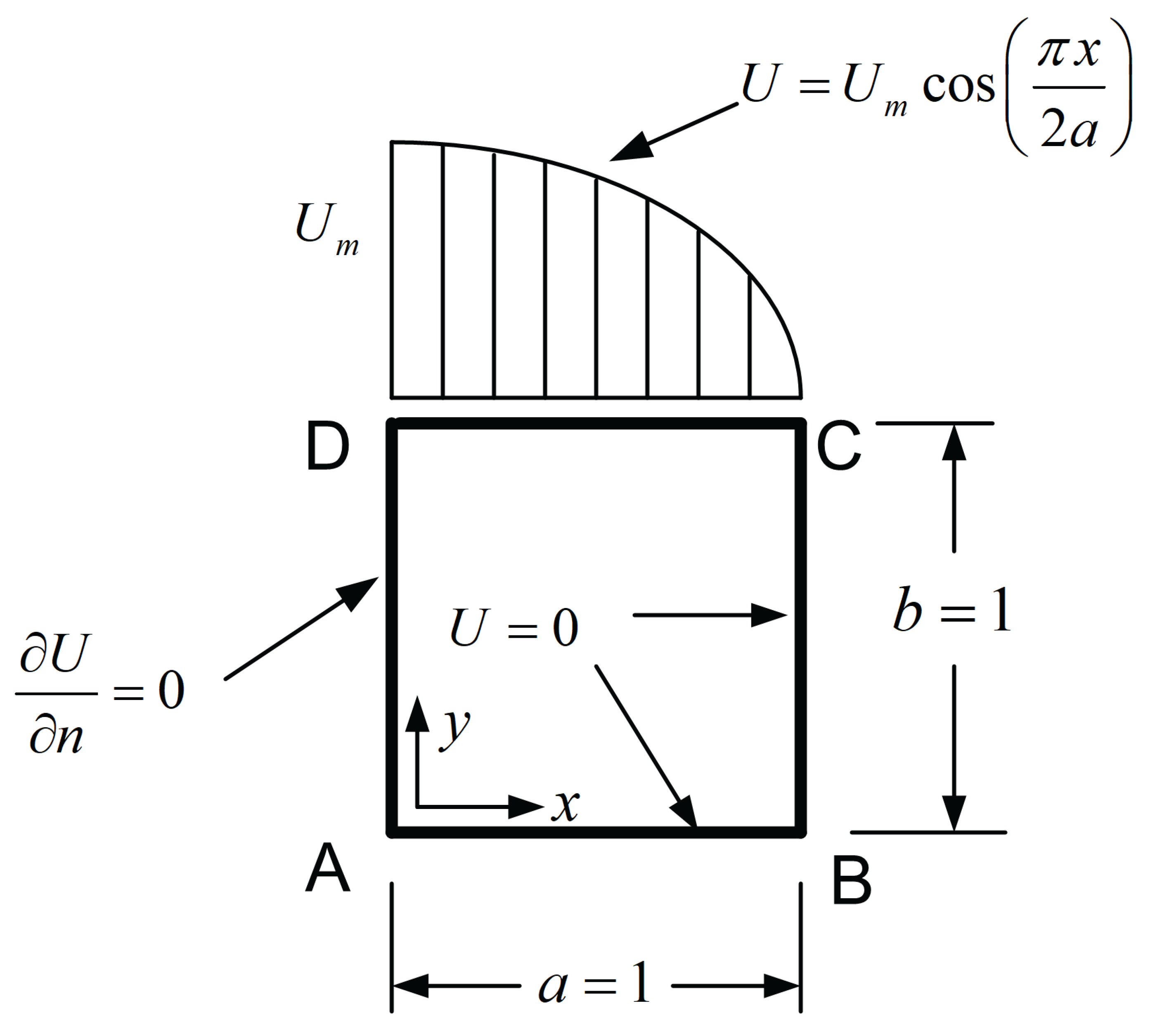
Figure 17.
Sum of basis functions in the conventional T-spline, before normalization.
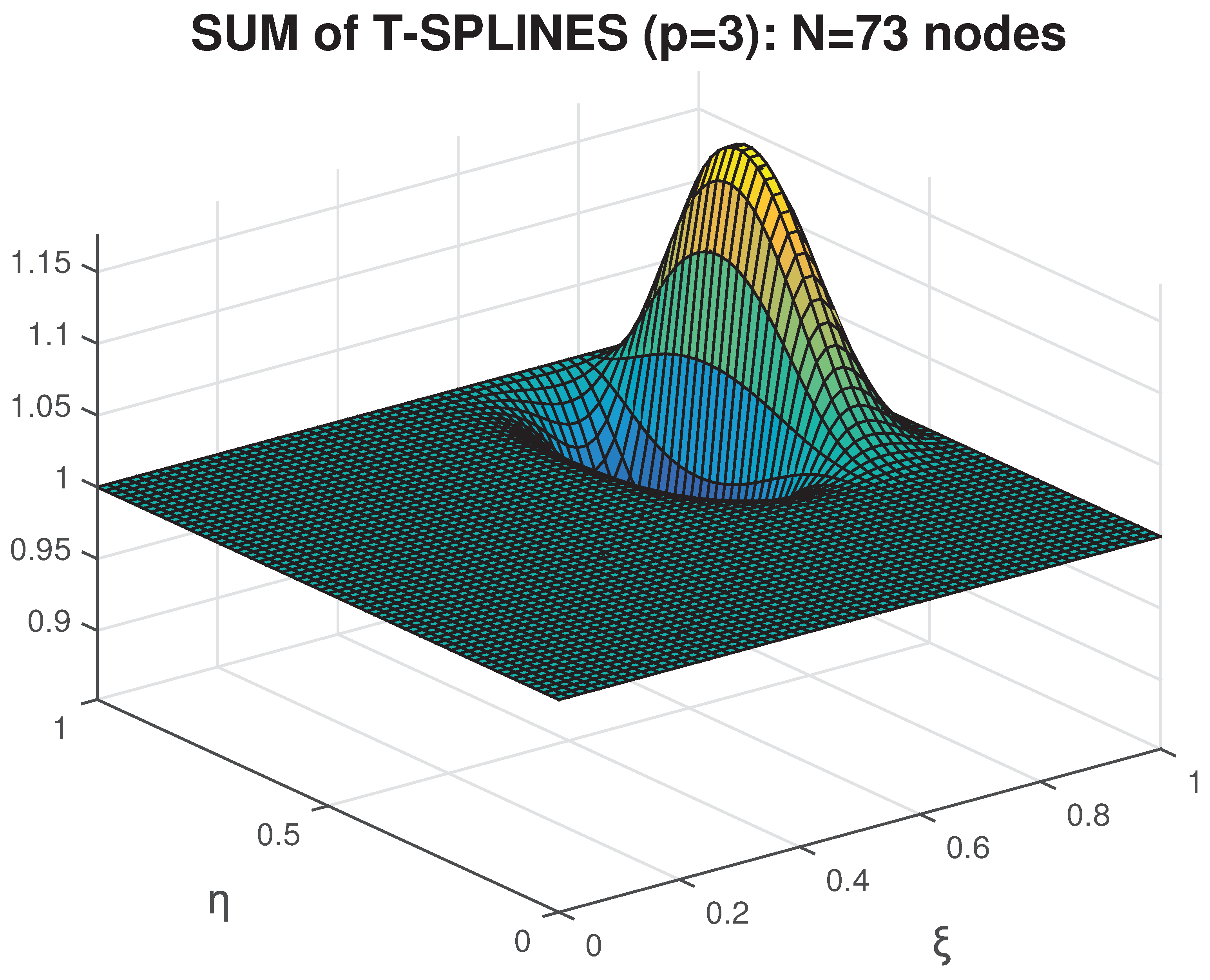
Figure 18.
Coons elements.
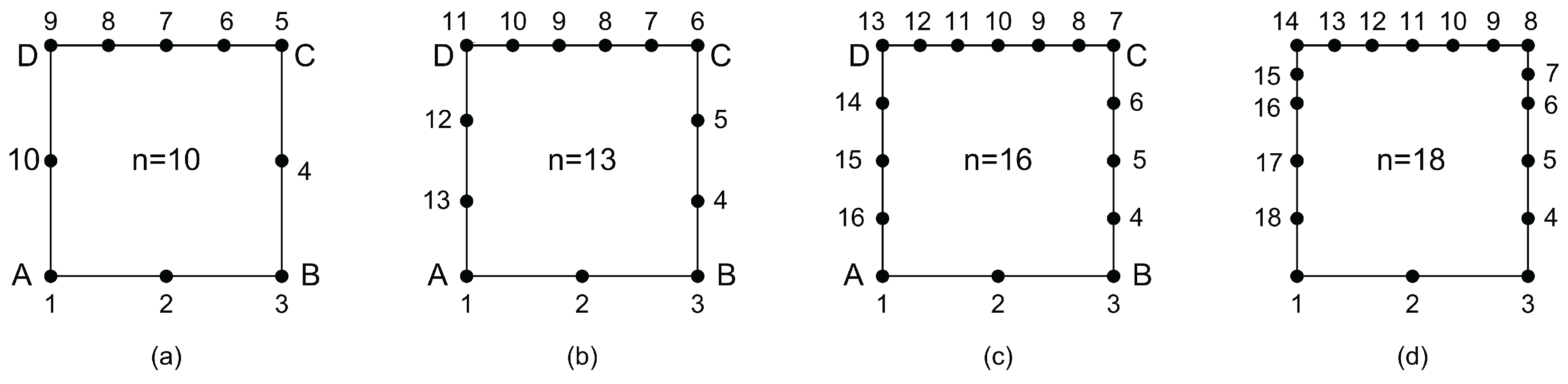
Figure 19.
Half-Annulus ().
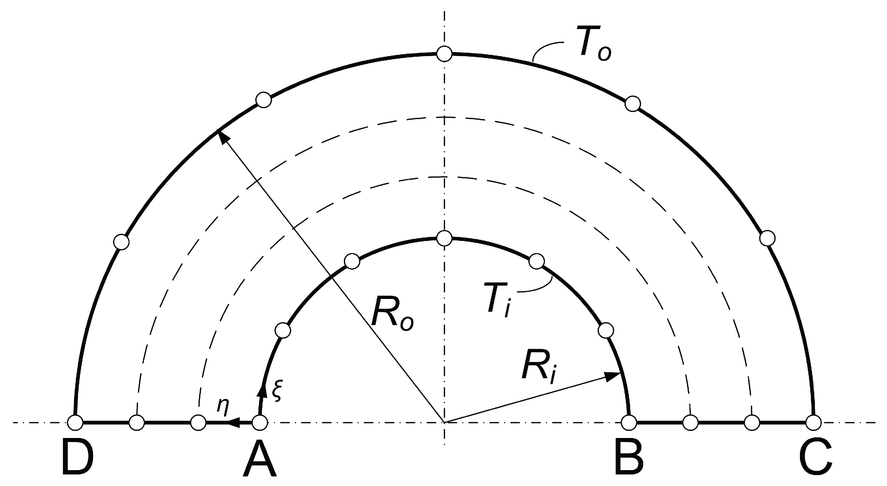
Figure 20.
Convergence quality of numerical solution for the circular ring.
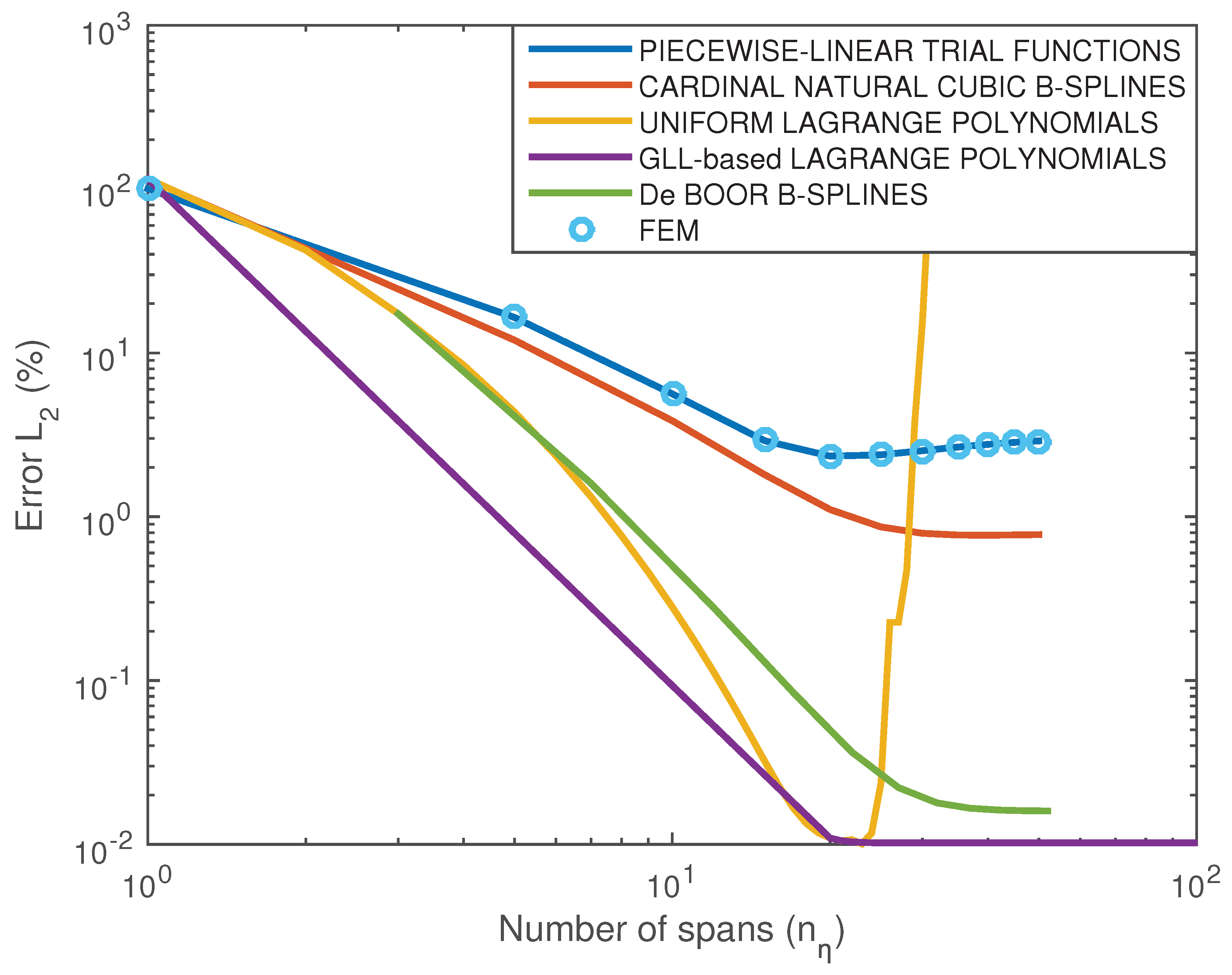
Figure 21.
Tensor-product and T-mesh control points of half-annulus: (a) Tensor product (81 DOFs): B-spline elements and control points (×). (b) T-mesh (80 DOFs). (c) T-mesh (76 DOFs). (d) T-mesh (73 DOFs).
Figure 21.
Tensor-product and T-mesh control points of half-annulus: (a) Tensor product (81 DOFs): B-spline elements and control points (×). (b) T-mesh (80 DOFs). (c) T-mesh (76 DOFs). (d) T-mesh (73 DOFs).
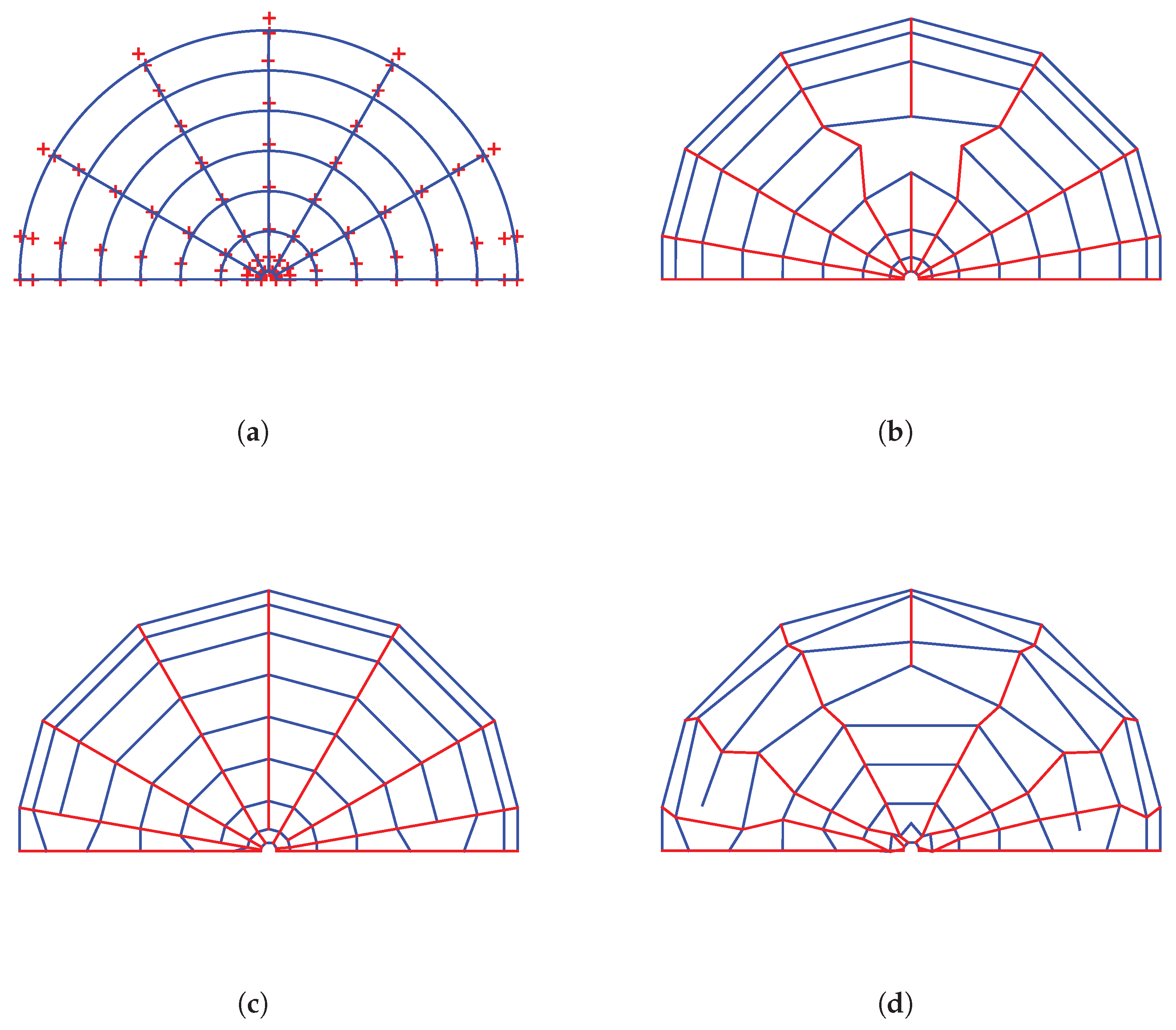
Table 1.
Errors ( in %) for the Classical Transfinite Elements shown in Figure 3.
Table 1.
Errors ( in %) for the Classical Transfinite Elements shown in Figure 3.
| Element type | Model-1 (Lagrange) | Model-2 (Natural B-spline) | Model-3 (De Boor B-spline) |
|---|---|---|---|
| 21-node | |||
| 27-node | |||
| 33-node | |||
| 113-node |
Table 2.
Errors ( in %) for the Unidirectional Elements shown in Figure 5.
Table 2.
Errors ( in %) for the Unidirectional Elements shown in Figure 5.
| Element type | Lagrange | Bernstein | De Boor B-spline |
|---|---|---|---|
| 12-node | 2.6671 | 2.6654 | 2.6704 |
| 18-node | 0.1638 | 0.1556 | 0.1567 |
| 25-node | 0.0385 | 0.0192 | 0.0273 |
| 32-node | 0.0327 | 0.0039 | 0.0173 |
| 32-node | 0.0327 | 0.0039 | 0.0182 |
a Nodes 19–25 uniformly distributed; B-spline knot vector: . b Nodes 19–25 non-uniformly distributed; B-spline knot vector: .
Table 3.
Errors ( in %) for the 27-node element shown in Figure .
| Lagrange | Bernstein | De Boor B-spline |
|---|---|---|
| 0.0191 | 0.0126 | 0.0245 |
Table 4.
Errors and condition numbers of proposed T-spline transfinite elements using de Boor B-splines.
Table 4.
Errors and condition numbers of proposed T-spline transfinite elements using de Boor B-splines.
| 81-node | 80-node | 76-node | 73-node | |
|---|---|---|---|---|
| (in %) | ||||
| Condition number | 54.2 | 38.1 | 61.2 | 43.2 |
Table 5.
Errors and Condition numbers for conventional normalized T-spline.
| 81-node | 80-node | 76-node | 73-node | |
|---|---|---|---|---|
| (in %) | 5.6581 | 0.0454 | 0.0011 | 0.1030 |
| Condition number | 54.2 | 39.8 | 61.2 | 51.8 |
Table 6.
Errors ( in %) of Coons-patch elements using uniform Lagrange polynomials as trial functions, and two alternative sets of blending functions.
Table 6.
Errors ( in %) of Coons-patch elements using uniform Lagrange polynomials as trial functions, and two alternative sets of blending functions.
| First set: | Second set: | ||||||
|---|---|---|---|---|---|---|---|
| 10-node | 13-node | 16-node | 18-node | 10-node | 13-node | 16-node | 18-node |
Table 7.
Errors ( in %) of classical transfinite elements using Lagrange or Bernstein polynomials (half-annulus).
Table 7.
Errors ( in %) of classical transfinite elements using Lagrange or Bernstein polynomials (half-annulus).
| 21-node | 27-node | 33-node | 113-node |
|---|---|---|---|
| 8.5839 | 4.3548 | 2.0773 | 0.1127 |
Table 8.
Errors and condition numbers for proposed T-spline elements (Half annulus).
| 81-node | 80-node | 76-node | 73-node | |
|---|---|---|---|---|
| (in %) | 1.0494 | 1.0521 | 1.3590 | 1.7091 |
| Condition number | 72.6 | 51.8 | 71.0 | 47.5 |
Table 9.
Errors and condition numbers for conventional normalized T-spline (Half annulus).
| 81-node | 80-node | 76-node | 73-node | |
|---|---|---|---|---|
| (in %) | 1.0494 | 1.0264 | 1.3428 | 1.6424 |
| Condition number | 72.6 | 54.4 | 71.2 | 64.9 |
Table 10.
Errors ( in %) of calculated eigenvalues using a single 73-node T-spline element (Rectangular cavity).
Table 10.
Errors ( in %) of calculated eigenvalues using a single 73-node T-spline element (Rectangular cavity).
| MODEL | Mode-2 | Mode-3 | Mode-4 | Mode-5 | Mode-6 | Mode-7 | Mode-8 |
|---|---|---|---|---|---|---|---|
| Proposed | 0.0002 | 2.3244 | 0.0002 | 0.0003 | 0.1028 | 0.5887 | 0.0657 |
| Conventional | 0.0267 | 2.1646 | 0.0002 | 0.0091 | 1.2588 | 0.5946 | 0.5847 |
Table 11.
Errors ( in %) of calculated eigenvalues using tensor-product and conventional FEM (81 nodes).
Table 11.
Errors ( in %) of calculated eigenvalues using tensor-product and conventional FEM (81 nodes).
| MODEL | Mode-2 | Mode-3 | Mode-4 | Mode-5 | Mode-6 | Mode-7 | Mode-8 |
|---|---|---|---|---|---|---|---|
| Tensor-product | 0.0001 | 0.0054 | 0.0001 | 0.0001 | 0.1021 | 0.0024 | 0.0649 |
| FEM | 1.2916 | 5.2387 | 1.2916 | 1.2916 | 4.9061 | 9.9833 | 8.0973 |
Disclaimer/Publisher’s Note: The statements, opinions and data contained in all publications are solely those of the individual author(s) and contributor(s) and not of MDPI and/or the editor(s). MDPI and/or the editor(s) disclaim responsibility for any injury to people or property resulting from any ideas, methods, instructions or products referred to in the content. |
© 1996 by the author. Licensee MDPI, Basel, Switzerland. This article is an open access article distributed under the terms and conditions of the Creative Commons Attribution (CC BY) license (https://creativecommons.org/licenses/by/4.0/).
Copyright: This open access article is published under a Creative Commons CC BY 4.0 license, which permit the free download, distribution, and reuse, provided that the author and preprint are cited in any reuse.


