
Submitted:
21 November 2024
Posted:
22 November 2024
You are already at the latest version
Abstract
This paper shows that the accuracy in T-spline based isogeometric analysis may be substantially improved by increasing the multiplicity of the inner knots up to the polynomial degree. This task can be performed considering the Bézier extraction operator matrix elementwise, and thus easily receiving an increased number of updated control points in the geometrical and computational model. Nevertheless, after the determination of the unique control points, sometimes the Bézier elements near the T-junctions may not be well-shaped, and thus minor automatic interventions are required to ensure full (i.e., C0 and G0) compatibility. The improved IGA solution may be also used as a reference to determine the a-posteriori error estimations in the T-spline elements of the domain. The methodology is shown in BVPs dominated by Laplace-Poisson equations in rectangular and curvilinear domains, while eigenvalues were extracted in a rectangular acoustic cavity.
Keywords:
isogeometric analysis
; T-splines
; Bézier extraction operator
; C0-G0 continuity
; potential problems
; Laplace equation
; eigenvalue problem
MSC: 65N06; 65B99
1. Introduction
Isogeometric analysis is today's research frontier in computational methods for the solution of BVPs and eigenvalue (Sturm-Liouville) problems. According to this method, the domain is decomposed into smaller patches, which are based on tensor-product NURBS approximation [1]. Later, the method was implemented in conjunction with T-spline approximation [2]. While in both these cases the basis functions may be computed as tensor products, which are based on either global or local knot vectors, it has been proposed to implement Bézier extraction (BEXT) operator instead [3,4].
The main advantage is that Bézier extraction, compared to the original implementation of IGA given in Ref. [1], is such that apart from the coefficients of the extraction operator, the basis functions are identical for all elements in the mesh as is the case for classical finite elements. Therefore, there is no need to implement B-spline (basis) function evaluation routines which are costly, from a numerical point of view. Another practical reason for using BEXT is that it reduces the communication errors of data transfer between the geometric model and the analysis.
On the other hand, the BEXT operator is a matrix which, when multiplied by the original control points of the T-mesh, provides a greater number of new (updated) control points, which have not been exploited to date. In this paper, we propose the utilization of the new control points, which form Bézier elements of C0-continuity, to automatically solve a parallel BVP. The latter solution is generally more accurate for the same number of elements, as those in the original T-spline, and therefore may be used as a reference in an a-posteriori error estimator.
2. Conventional IGA Procedures
2.1. Tensor-Product of Local Knot Vectors (MODEL-1)
It is well known that for two given global knot vectors associated with a patch, the tensor product B-spline (or NURBS) functions can be determined using Cox-de Boor recursion [5,6]. The same can be performed in T-spline approximation, with the only exception that the tensor product is based on local knot vectors associated with anchors.
For the sake of simplicity, we reduce ourselves to cubic T-splines (i.e. with polynomial degree p = 3). Therefore, in a usual T-spline it is sufficient to construct a matrix, called (say) Uvec, which for each anchor ‘α’ determines the knots of those other anchors at the left and the right of that under consideration, and thus forming the local knot vector Ξα = {ξ1, ξ2, ξ3, ξ4, ξ5}. Similarly, we need another matrix, called (say) Vvec, which determines the knots of those anchors at the bottom and the top of that under consideration, and thus forming the local knot vector Hα = {η1, η2, η3, η4, η5}. Again, for p = 3, the matrix Uvec (and similarly Vvec) is of size nα × 5, where nα is the number of anchors in the T-patch. Based on these two matrices as input, for each couple (ξ, η) of the T-patch, we can determine the tensor product of B-splines, Nα,p(ξ) Nα,p(η).
The abovementioned B-spline functions, Nα,p(ξ) and Nα,p(η), can be easily calculated using the function spcol included in MATLAB®, but also open-source software is available in many repositories and books (e.g. [7]).
Moreover, in the case of p = 3, for any set of five nondecreasing knots {x1, x2, x3, x4, x5}, which may be a single row from the abovementioned matrix Uvec, there is a single piecewise cubic B-spline function Nα(x), which analytically is given by (see, e.g., Ref. [8]):
In general, the independent variable x and the knots x1 to x5 shown in Equation (1) may represent either of parameters ξ or η, as well as the knots involved in the abovementioned local knot vectors Ξα = {ξ1, ξ2, ξ3, ξ4, ξ5} and Hα = {η1, η2, η3, η4, η5}. Therefore, for each anchor ‘α’, Equation (1) applied to Ξα determines one B-spline Nα(ξ) and applied to Hα produces Nα(η). The range of the non-vanishing tensor-product bivariate basis function is the rectangle [ξ1,ξ5]×[η1,η5]. In general, a weight is associated to the anchor .
Based on the above B-spline functions Nα(ξ) and Nα(η), for each anchor ‘α’ we can calculate the bivariate blending function Bα(ξ, η) = Nα(ξ) Nα(η). When the patch is curvilinear, each anchor is also associated to a weight wα. Following the notation in Ref. [2], if ‘A’ is the set of all the anchors into the patch, we define the blending functions as follows:
Clearly, the numerator of Equation (2) represents a weighted tensor product of the local B-spline functions associated to the anchor ‘α’. The denominator W(ξ,η) represents the sum of the weighted tensor products due to all the contributed anchors, and is set to ensure the Partition of Unity Property at every point (ξ,η) of the parametric space:
Based on the above blending functions within a curvilinear patch, and given the control points , the T-spline in physical space is described by:
It is instructive to recall that in the special case of a NURBS tensor product of degree p = 3, the abovementioned set ‘A’ consists of exactly (p + 1)2, i.e. sixteen, nonzero bivariate basis functions which fulfil Equation (3). In contrast, in a sub-patch of a T-spline, there may be more than 16 non-vanishing bivariate blending functions. Regarding an annulus, Ref. [4] shows most T-elements are influenced by 16 and a few of them by 17 blending functions.
As discussed above, regarding a certain T-element it is possible that a part of it be influenced by 16 non-vanishing basis functions whereas another part by 17 ones. Moreover, another possibility is that the same number (say 16), but different basis functions may dominate in different parts of the same element. In all these cases, we talk about “reduced continuity”, and to make these elements be suitable for isogeometric analysis, it becomes necessary to subdivide them, and thus an increased number of T-elements is produced. Then, we talk about “Analysis Suitable T-splines” (AST).
After the creation of analysis-suitable T-elements, the blending functions of Equation (2) may be used to estimate the mass and stiffness matrices associated with the T-patch under consideration.
2.2. The Standard Utilization of the Bézier Extraction Operator (MODEL-2)
Despite the ease in the implementation of Equation (1), and although numerical evaluations may be easily performed using open-source libraries or proprietary libraries, the tendency is to utilize the Bézier extraction (BEXT) version. The basic theory is given below.
In the theory of computer-aided geometric design (CAGD), it is well known that knot insertion does not alter the shape of a curvilinear patch, both in shape and parametrically [7]. For one-dimensional interpolation of a curve C(ξ) with p = 3, initially we have C2-continuity at the inner knots, and after one knot insertion it decreases to C1-continuity. Continuing with a second knot insertion at the inner knots (thus three equal knots in total, i.e. equal to degree p), the continuity further decreases to C0. Therefore, when the multiplicity λ of inner knots becomes equal to the polynomial degree p, we obtain C0-continuity at the inner knots.
Moreover, for a two-dimensional NURBS patch, the above procedure is again applicable, but then the multiplicity of inner knot should become λ = p2, so that C0-continuity is obtained in both directions. As shown in Ref. [3], the column-vector including the non-zero B-spline (basis) functions Ne is related to the extracted Bernstein polynomials stored into the column-vector Be per element, through the formula:
where Ce is the Bézier extraction operator matrix, which corresponds to the e-th B-spline tensor-product element. In general, in a NURBS patch, Ce is a matrix of size (p + 1)2 × (p + 1)2 whereas Ne and Be are column-vectors of size (p + 1)2 × 1, due to the local support property of B-splines.
Ne(ξ,η) = Ce.Be(ξ,η),
In a similar way, for a two-dimensional T-spline patch, Scott et al. [4] presented a pseudocode and showed that multiple knot insertion leads to the so-called Bézier extraction operator matrix, Ce, which may be used to estimate the C2-continuous blending functions of the T-spline element assembly.
In more detail, given the initial control points and their weights of the C2-continuous e-th T-spline element, the above-mentioned multiple knot insertion alters the initial weights according to the formula:
In Equation (6), denotes the updated element weights after the multiple knot insertion, whereas are the initial given element weights which are associated to the initial control points .
As we mentioned earlier, within a T-mesh there may be some sub-patches of reduced continuity, and this has been a matter of intensive research [9]. To ensure uniqueness and then perform accurate numerical integration, it becomes necessary to elongate some edges of the T-mesh, and thus obtain an analysis-suitable T-mesh. Nevertheless, although this procedure leads to an increased number of analysis-suitable T-elements, not always a standard number of non-vanishing blending functions is ensured.
As we shall see later, in the benchmark test of the annulus (Example 3), which has been studied in Ref. [4], most of the elements are influenced by (p + 1)2 = 16 nonzero basis functions, but also there are two elements which are influenced by 17 ones. This in turn means that, for most elements, the Bézier extraction operator matrix Ce will be of size 16 × 16, but in some of them will be of size 17 × 16.
For the sake of completeness, the computation of the blending functions is performed as follows:
From Equation (2) one may observe that the bivarate blending functions R(ξ,η) are tensor products of local univariate basis functions, properly normalized, as follows:
where the denominator is the so-called “weighting function”. Each blending function is associated to an anchor , which for the polynomial degree p = 3 is a true control point.
At a certain point (ξ,η) of the T-patch, there is a number of ‘’ nonzero bivariate basis functions, near round the value (p + 1)2 (e.g., n = 16, 17, …).
Dropping out the subscript ‘e’ denoting the element under consideration, if is the diagonal matrix which includes all the above ‘’ involved weights,
and is the column-vector (of size ) of all the bivariate B-spline functions affecting the element under consderation, then Equation (7) is rewritten in a matrix form which provides the rational column-vector [of size ],
To obtain the blending functions, we still need to calculate the weighting function , which is involved in the denominator of Equation (9). The latter is written as
Substituting the B-spline column-vector N from equation (5) into equation (10), the latter becomes
Substituting equation (6) into equation (11), we receive:
where is a column-vector of standard size 16 × 1, including the weights associated to the Bézier-Bernstein basis functions. Substituting equations (5) and (12) into equation (9), we eventually receive:
where is the diagonal matrix including the initial weights of the control points in the C2-continuous model (cf. equation (8)). Equation (13) dictates that it is not necessary to directly calculate the B-spline functions, either through the recursive (Curry-Schoenberg 1966) formulas or using the analytical ones given by equation (1), but only the extraction matrix C, which depends only on the knot vectors, while the expressions of the tensor-product Bernstein polynomials is trivial.
Based on the blending functions given by Equation (13), the computation of the mass and stiffness matrices is straight forward.
3. The Proposed Computational Procedure (MODEL-3 and MODEL-4)
3.1. General Theory (MODEL-3)
Although Ref. [4] has focused on the estimation of the C2-continuous blending functions according to the BEXT Equation (13), for the purposes of the present paper below we focus on the updated control points as well.
In more detail, given the initial set of control points and their associated weights in the C2-continuous T-spline model, the multiple knot insertion until the multiplicity becomes equal the degree p, provides additional control points according to the formula:
In Equation (14), the superscript ‘w’ indicates projective coordinates, i.e., Cartesian coordinates multiplied by the associated updated weight, whereas the superscript ‘T’ indicates the transpose of the BEXT matrix Ce. Moreover, as previously mentioned in section 2.2, in Equation (6), denotes the updated weights of the new control points Q (after the multiple knot insertion), whereas are the initially given weights associated to the initial control points P. Note that the superscripts {Q} and {P} were set only to clearly indicate the status after and before knot insertion, respectively.
Regarding the size of the arrays involved, we repeat that the element Bézier extraction operator matrix Ce includes so many rows as the number of the non-vanishing blending functions within the T-spline element (e.g. 16, 17, etc), whereas the number of columns is standard, equal to 16. Therefore, in general, Ce is a non-square matrix. Concerning the element vector of control points and the associated vector of element weights in the initial C2-continuous model, each of them has so many rows as exactly the matrix Ce (i.e., 16, 17, etc). Interestingly, whatever the number of rows in Ce is, the resulting number of updated control points in the C0-continuous Bézier element equals (p + 1)2 = 16.
The applied algorithm of the present paper is as follows:
- Based on the initial nP control points P and the given index space, create nele analysis-suitable T-spline elements.
- Apply the BEXT matrix Ce in each of the above nele T-spline elements, and thus determine:
the updated control points Qe, and
the associated weights .
Find the unique control points (Qe)unique among the above Qe (initially including nQ’ = 16nele points), and thus determine the final number of nQ control points, which fully define the nele rational Bezier elements. An instructive example is presented in section 3.3. Alternatively, one could implement a variation of the Oslo algorithm [10], which is a recursive procedure to simultaneously handle multiple knot insertion.
Apply the weighted tensor products of Bernstein polynomials [B1 = (1-s)3, B2 = 3(1-s)2s, B3 = 3(1-s)s2, B4 = s3] to determine the rational bivariate basis functions within each rational Bézier element and calculate the element mass and stiffness matrices. Note that always there are npts = 16 control points in each Bézier element, and thus for potential problems each element matrix is of size 16 × 16.
Build the total matrices of the entire T-patch, apply the boundary conditions and solve the equations system to determine the unknown coefficients.
As we demonstrate below in the four examples of the present paper, the final number, nQ, of control points in the proposed C0-continuous model, is larger than the initial number of nP control points in the C2-continuous one. By analogy to the tensor-product NURBS model, below a closed-form expression will be provided for the quantity nQ.
3.2. Estimation of Control Points nQ for C0-Continuity
To establish the procedure for the estimation of the updated control points Q which are produced by the BEXT process, we resort to the conventional tensor-product B-spline approximation. For the sake of simplicity, we consider the piecewise cubic tensor-product B-spline patch shown in Figure 1a (of degree p = 3), for the unidirectional knot vector:
U = [0,0,0,0, 1/3,2/3, 1,1,1,1]
Based on trivial computer-aided geometric design (CAGD)-theory [7](p.66), the number of control points per direction is given by
where m is the number of elements in the knot vector U. Since in Equation (15) there are m = 10 knots and p = 3, we have n = 6 per direction, which means nP = n2 = 36 control points in the entire two-dimensional patch.
n = m – p –1,
After double knot insertion at the nin = 2 inner knots, as required by BEXT [7](p.161), the number of control points per direction becomes:
and therefore, the total number of the updated control points {Q} after BEXT will be:
n’ = n + nin (p – 1) = 10,
nQ = n’2 = 102 = 100.
Below, the same result will be derived, considering now the tensor-product B-spline patch as a T-spline patch. The conclusions of this approach will be extended to T-spline patches as well.
Obviously, the above two-dimensional B-spline patch, described by Equation (15), is equivalent to a T-mesh with six anchors per direction, and thus forming the following Index Space:
Ax = Ay = {0, 0, 1/3, 2/3, 1, 1} = {ξ1, ξ2, ξ3, ξ4, ξ5, ξ6}.
The set of anchors in Equation (19) are denoted by blue-colored lines in Figure 1b. The BEXT procedure requires the knot insertion at the inner knots such as ξ3 = 1/3 and ξ4 = 2/3, until the multiplicity becomes λ = p = 3. This demands the introduction of the red-colored lines shown in Figure 1b, where one may distinguish three different types of knots, as follows:
- Type A: Knots related to the corners of the patch (4 corners with 4 anchors per corner).
- Type B: Knots related to intermediate places along the four edges, not coinciding with the corners (6 anchors per initial knot).
- Type C: Knots related to initial knots in the interior of the patch (9 anchors per initial knot).
Based on the above categorization, for the case shown in Figure 1b, in which there are 4, 6, and 9 initial knots of categories A, B, and C, circled respectively, we have:
Anchors at the corners: 4 × 4 = 16 (20a)
Anchors along boundaries: 8 × 6= 48 (20b)
Anchors in interior: 4 × 9 = 36 (20c)
SUM of anchors in the patch: nQ = 100, Q.E.D. (20d)
A similar procedure, to determine the number nQ, may be followed for a T-mesh, which is again divided into the above three categories, A, B, and C. The only minor exception concerns elements of reduced continuity, in which extra inner knots are added in the index space, by extending existing connecting lines, as mentioned earlier. Depending on the location of these extra points, which may also be classified as Type C, the full number ‘9’ or part of it may be applied to them.
3.3. On the Uniqueness of Control Points
Let us continue working with the nine tensor-product B-spline elements illustrated in Figure 1, which are based on the univariate knot vector of Equation (15).
For this configuration, the initial (nP = 36) control points are shown in Figure 2(a), whereas those (nQ = 100) after multiple knot insertion in Figure 2(b). One may observe that, after the multiple knot insertion, each of the nine Bézier elements is occupied by 4 × 4 = 16 control points. Obviously, the number of the actual nQ = 100 control points differs from the blind product nQ’ = 9 elements × 16 control points per element = 144.
The above discrepancy, between the erroneous nQ’ = 144 and the correct nQ = 100, is due to the following reasons:
- Each of the four control points at the intersections between horizontal and vertical inter-element boundaries (illustrated in Figure 2b by red circle: 🔴), belongs to four elements, while must be countered only once. Therefore, instead of the blind number 4 × 4 = 16, we must consider only 4 of them, which means that we have 12 additional fictitious points to subtract from 144.
- Each of the thirty-two control points along the inter-element boundaries (illustrated in Figure 2b by red cross: x), belongs to two elements, and therefore a blind computation would results in 32 × 2 = 64 points. To obtain the exact number, half of them (i.e., 32) must be subtracted from 144.
Therefore, the total fictitious number of the additional control points is 12 + 32 = 44. When the latter (44) is subtracted from the blind number nQ’ = 144, we obtain the correct number nQ = 100.
3.4. Fixing C0 and G0-Incompatibilities (MODEL-4)
Although the procedure discussed in section 3.1 (MODEL-3) is straight-forward, sometimes there are minor shortcomings to be corrected before analysis is performed. In this context, it may happen that within a sub-patch there is “reduced continuity”, and thus partitioning is necessary. For example, in the test case of Ref. [4](p.134), it was shown that among 24 elements, 22 of them are affected by 16 whereas the rest two by17 control points.
In the framework of the present paper, it was found that after the partitioning of the sub-patches having reduced continuity, compatibility problems may appear in their neighborhood. For example, the reduced continuity of the sub-patch (I) in Figure 3a demands its subdivision, into I(a) and I(b). Although the produced Bézier elements (I(a) and I(b)) are well formed, their neighboring Bézier element (II), which shares the common edge BE with the sub-patch (I) of reduced continuity, is not compatible (see also, Figure 3b). Clearly, this happens although the Bézier element (II) is fully continuous. Although sometimes the accuracy of the numerical solution may be sufficient ignoring the incompatibility, in general it becomes imperative to perform a further tessellation on the largest element (II), as shown in Figure 3c. The procedure of this tessellation is easy and is based on the common edge considered from the side of the element (I) of reduced continuity. A full description of the applied numerical scheme is given in Appendices A and B.
4. Matrix Formulation
Numerical results refer to potential problems, particularly to Laplace equation and wave propagation equation. The latter partial differential equation is written as:
(1/c2)∂2u/∂t2 - ∇2u = 0,
Based on any set of control points (P or Q) associated with blending functions RPQ (column-vector) in general, the matrix formulation of IGA is:
where the stiffness and mass matrices as given by the following domain integrals:
and
Mass matrix: M = (1/c2)∫RPQ (RPQ)t dA,
Stiffness matrix: K = (1/c2)∫∇RPQ (∇RPQ)t dA,
Obviously, Laplace equation (∇2u = 0) is a special, steady-state, case of Equation (22), and thus is described by the matrix equation
where the force vector is given as
Regarding the numerical extraction of the eigenvalues (λ = ω2) of an acoustic cavity, we use the following formula:
5. Results
The theory is supported by four examples. The first two examples are simple rectangles and have been devised to need edge extension in the same direction at two places to ensure analysis-suitable T-splines. The third example refers to an annulus and follows the pattern of Ref. [4], which requires again two edge extensions but now in mutually perpendicular directions. The fourth example has a similar index space to that of the annulus but refers to a rectangular domain.
Each example was solved using four models, as follows:
MODEL-1: B-spline functions N were calculated as local tensor-product associated to control points P, using de Boor’s spcol MATLAB® function; equation (1) is also applicable as an alternative. Furthermore, weights and normalization were imposed to obtain the final blending functions R.
MODEL-2: B-spline functions N were calculated using Bézier extraction operator matrices, , associated to initial control points P. Furthermore, weights and normalization were imposed to obtain the final blending functions R.
MODEL-3: Basis functions B (Bézier-Bernstein polynomials) are known functions and were combined with the new control points Q on the Bézier elements of C0-continuity.
MODEL-4: When MODEL-3 leads to inter-element incompatibility like that demonstrated in Figure 3, the larger Bézier element is subdivided according to Appendix A and Appendix B, thus eventually producing the further updated set of control points Q’ which is slightly larger than Q. Based on the further corrected weights wQ’ and the further updated set of control points Q’, we construct the new rational Bernstein polynomials B’ which constitute the final set of basis functions.
By theory, MODEL-1 and MODEL-2 are identical, because they only use a different computational procedure to calculate the same B-spline functions N, associated to the same control points P, at the same Gauss points. The only reason that MODEL-2 is separately mentioned here, is because it crosschecks the accuracy of the computer code and thus increases confidence.
In each example, for the first three models (MODEL-1 to MODEL-3), the number of (T-spline or Bézier) elements and the number of Gauss points is the same. Nevertheless, the number of the involved DOFs of MODEL-3 differs from those of (MODEL-1 and MODEL-2), i.e. always we have nQ > nP, as was explained in sections 3.1 and 3.2.
Furthermore, in MODEL-4 the number of elements is larger by those subdivided, whereas the number of DOFs (nQ’) is slightly larger than nQ.
In steady-state problems (Laplace equation), the accuracy of the models was expressed in terms of the L2-norm in percent (%), using the following formula:
All computations were performed on the same PC, using MATLAB® R2018.
5.1. EXAMPLE 1: Vertical Heat Flow
In the rectangular domain of size L × H = 7 × 4, of which the index space is shown in Figure 4, the temperature is prescribed on the bottom and top edges, as follows: (y = H) and (y = 0), while the vertical edges at x = 0 and x = L are fully insulated .
One may observe in Figure 4 that the index space includes nP = 56 anchors and 19 initial patches. However, to ensure continuity, it becomes necessary to extend the edge 19-20 by two units to the right (and thus producing the new points 1 and 2, connected by dashed line), and to extend the edge 38-37 to the left (and thus producing the new points 3 and 4, connected again by dashed line). In this way, the number of degrees of freedom (DOF) remains the same at nDOF = 56, but due to the two subdivisions (each by two units), the number of T-spline elements in which Gauss integration will be performed increases, from the initial 19 to eventually nele = 23.
The numerical solution using MODEL-1 and MODEL-2, which is associated to the system of nDOF = 56 DOF shown in Figure 4, was found to coincide with the exact solution, , with .
Regarding the formation of Bézier elements produced after multiple knot insertion using BEXT (which compose MODEL-3), one may observe in Figure 5 two shortcomings regarding compatibility, as follows. The first shortcoming concerns the element at the upper left corner along the edge (31-43 in Figure 4, 108-159 in Figure 5) and the second refers to the element in the lower right corner along the edge labelled (14-26 in Figure 4, 43-64 in Figure 5). Nevertheless, the numerical solution of MODEL-3 (nQ = 244 DOF) was also found to coincide with the exact solution. It is hypothesized that this happens because the heat flow is vertical, and the existing vertical edges do not interrupt the continuity of the interpolation. It is worth mentioning that the implementation of MODEL-4 (not shown but explained in Example 2) did not change the excellent result of MODEL-3 at all.
It is worth mentioning that the number of nQ = 244 control points could be predicted by classifying the anchors into three categories according to section 3.2. Thus, considering (A: 4 corners, B: 14 intermediate anchors on boundary, and C: 9 internal anchors including the extra ones produced after extension), the result nQ = 244 is shown in Table 1.
The distribution of the temperature using MODEL-3 is shown in Figure 6, but it is the same in all the four models.
5.2. EXAMPLE 2: Horizontal Heat Flow
The same geometric model as that of Example 1, is now solved under different Dirichlet boundary conditions: and on the vertical edges, whereas the bottom and top edges are now thermally insulated (). Obviously, the heat flow is horizontal, and the exact solution is given by with .
Again, the T-mesh is the same as that shown in Figure 4, whereas the obtained set of nele = 23 Bézier elements after Bézier extraction is again that shown in Figure 5 (for MODEL-3).
As previously happened, again in Example 2, MODEL-1 and MODEL-2 resulted in zero errors all over the domain, as shown in Figure 7.
Nevertheless, now, the average numerical error of MODEL-3 (Figure 5, 23 Bézier elements) is substantially large, equal to about 8.39%, as shown in Figure 8. This problematic result obviously happens because the heat flux is discontinuous when it passes through the incompatible vertical edge 108-159 in the large Bézier element at the upper left corner, as well as from the vertical edge 43-64 in the large Bézier element at the lower right corner.
To fix this error, we must ensure continuity along the two above-mentioned interfaces 108-159 and 43-64, by splitting the neighboring elements, and thus obtaining (nele)4 = 25 Bézier elements (extra 2, in addition to previously (nele)3 = 23 elements) associated to nQ’’ = 256 nodes (previously nQ = 244). This configuration defines MODEL-4, shown in Figure 9, which eventually leads to zero error (precisely, L2 = 4.91e-10 %). The distribution of the temperature for MODEL-4 is perfect, as shown in Figure 10.
5.3. EXAMPLE 3: Annulus
5.3.1. T-Spline Model
This example is a standard benchmark test [4], originated from Scott’s PhD thesis [11], for which all technical data (coordinates, weights) have been provided. It refers to an annulus of central angle 90 degrees, with internal radius R1 = 1.5 and external radius R2 = 3. The index space, for polynomial degree p = 3, is shown in Figure 11.
One may observe in Figure 11 that the index space consists of nP = 57 anchors, and those numbered ‘25’ and ‘33’ are of valence 3. Therefore, as previously, we must extend the associated central edge (’26-25’ and ‘25-33’, respectively) to recover the reduced continuity along the pseudo-lines ’25-1-2’ and ’33-3-4’, respectively. In this way, the initial 20 sub-patches increase to nele = 24 T-spline elements (note that those between double boundaries are of zero area and thus ignored). In more detail, the sub-patch bounded by the anchors ’19-20-32-31’ splits in ’19-20-1-2’ and ’2-1-32-31’. Similarly, the sub-patch ’20-21-33-32’ splits in ’20-21-25-1’ and ‘1-25-33-32’. Moreover, the sub-patch ‘32-33-34-41-40’ splits into ’32-33-3-40’ and ’33-34-41-3’. Finally, the sub-patch ’40-41-48-47’ splits into ’40-3-4-47’ and ‘3-41-48-4’. It is worth mentioning that, even after the final decomposition in nele = 24 C2-continuous elements, the number of DOFs remains at the initial nP = 57 anchors (the double anchors along the boundary are also included).
For the above model of nP = 57 DOF (MODEL-1 and MODEL2), the result is shown in Figure 12.
Moreover, in Figure 13 we present the nele = 24 Bézier elements associated to nQ = 247 unique nodes (MODEL-3), exactly as were produced using the Bézier extraction operator matrix. One may observe that the second element from bottom in the first column (also shown as ’18-19-31-30’ in Figure 11) is not compatible with its neighboring element (the edge ’19-2-31’ of Figure 11).
5.3.2. Tensor-Product Model
For the sake of completeness and sustain the tendency of the accuracy in the four models tested, we also present results obtained using the tensor-product using uniform knot distribution. More precisely, for both directions we used the uniform knot vector:
U = [0,0,0,0, 1/4,2/4,3/4, 1,1,1,1].
This means four uniform subdivisions per direction (both circumferential and radial) and thus nP = 72 = 49 DOFs, for MODEL-1 and MODEL-2.
Regarding MODEL-3 and MODEL-4, obviously they are identical, consisting of 4 x 4 = 16 Bézier elements, associated to nQ = 132 = 169 DOFs.
For all the four models, the results are shown in Table 3. One may observe here that, in contrast to the T-spline model (reported in Table 2), the MODEL-3 is superior to MODEL-1 and MODEL-2, because it also represents MODEL-4 which in all the previous cases was the best overall. However, we must consider that MODEL-4 used 3.4 times more DOFs than MODEL-1 and MODEL-2.
5.4. EXAMPLE 4: Rectangular Acoustic Cavity
We consider a rectangular cavity of size a × b = 3.5m × 1.5m, and wave velocity c = 1 m/s, under Neumann boundary conditions (∂u/∂n = 0). The closed-form analytical eigenvalues may be found in [12].
The index space is again that shown in Figure 11, and thus consists of nP = 57 anchors. All the four models were taken to be the same as those in Example 3.
For each separate acoustic mode, the error (in percent) was calculated according to the formula:
In Figure 15 we present the error of the first fifty calculated eigenvalues using MODEL-1 (57 DOFs, 24 elements), MODEL-3 (nQ = 247 DOFs, nele = 24 elements) and MODEL-4 (nQ = 256 DOFs, nele = 25 elements). One may observe the superiority of MODEL-4 in the entire spectrum of frequencies, mostly in the lower ones in which MODEL-3 (although better than MODEL-1 and MODEL-2) slightly underestimates the exact eigenvalues. Overall, one may observe that in this example, the tessellation of the one neighboring Bézier element did not seriously affect the quality of the numerical solution.
6. Discussion
It was shown that the control points which are implicitly involved in the Bézier extraction operator matrix, can serve as a vehicle to build rational Bézier elements of C0-continuity. Although this procedure is straight-forward in NURBS approximation, T-splines suffer from minor shortcomings, close to the borders of sub-patches with reduced continuity. Therefore, it becomes conditionally necessary also to subdivide the closest Bézier element to the previously subdivided elements of reduced continuity. For example, one exception to this rule is when the extension reaches the boundary layer, as shown in Figure 13, in which only one element needs to be tessellated (as eventually shown in Figure 14), despite there being two elements of reduced continuity.
It was found that the abovementioned tessellation is not always necessary, but strongly depends on the boundary conditions. In Example 1 concerned with vertical uniaxial heat flow, no tessellation was necessary to none of the two discontinuous Bézier elements, because the line of discontinuity did not influence the flow (was parallel to it). In contrast, in Example 2, with the same T-mesh but BCs leading to horizontal flux, the lines of discontinuity were perpendicular to the flow and thus influenced it much (8.4%). It is worth mentioning that when only the Bézier element to the top left part of the domain was tessellated, the average error decreased (from 8.4%) to only 7%, and this is attributed to the low average temperature within it. Eventually, when both discontinuous Bézier elements were subdivided, the overall error completely vanished.
The tessellation of the neighboring Bézier elements close to them (which constitutes MODEL-4), is a standard technique which was developed in the context of the present paper. After the tessellation, the neighboring rational Bézier elements are not only C0- but also G0-continuous, which means that they share the same control points. Although the results are found to be very encouraging, a shortcoming of this approach is the need for tessellation in the entire row of elements until the boundary of the entire patch is reached. To resolve this drawback, instead of the tessellation of the discontinuous Bézier element and those in the same row, a single transient element (i.e., the closest to the line of discontinuity) may be constructed [13,14].
In Example 3 regarding the annulus, the average error was small because, due to the small ratio of the radii, R1/R2=1/2, the logarithmic distribution of the temperature was almost linear in terms of the radius r. In this example, Table 2 clearly shows that MODEL-4 is the most accurate among the four models, all of them referring to the same number of nele = 24 T-spline elements. For the avoidance of any doubt, tensor-product (NURBS) analysis was added to elucidate this example (see, Table 3), because standard coordinates and standard weights may be applied for its reproduction by any researcher.
The superior accuracy of MODEL-4 dictates that it can take the role of a refence value for a-posteriori error estimation.
In principle, the proposed methodology is applicable to the entire spectrum of computational mechanics, including elasticity, where most part of research is focused [15].
7. Conclusions
Bézier extraction matrices, which is the golden standard in isogeometric analysis (IGA), may be used to construct updated unique control points which further determine a set of rational Bézier elements with C0-continuity characterized by more degrees of freedom than that in the standard IGA model. This in turn leads to a second numerical solution of higher accuracy, practically without affecting the number of T-spline elements, and thus useful for a-posteriori error estimation. It was found that in some cases, it is useful or necessary to further subdivide a small number of Bézier elements which share the same interface with T-spline elements of reduced continuity. Although in the present paper a standard tessellation of Bézier elements was applied, transient rational elements are also applicable. The applied methodology is generally applicable to the whole spectrum of computational mechanics as well as to three-dimensional problems.
The finding of the unique real root of the cubic polynomial in Equation (A.3) is a trivial task of numerical analysis, which may be facilitated using a mathematical package such as MATLAB®, using the commands coefficients = [a, b, c, d]; root_values = roots(coefficients); in conjunction with the condition find(root_values <1 & root_values >0);
Author Contributions
Conceptualization, C.P.; methodology, C.P. and J.D..; software, C.P. and J.D.; validation, C.P. and J.D.; writing—original draft preparation, C.P.; writing—review and editing, C.P.; visualization, J.D.; supervision, C.P.; project administration, C.P. All authors have read and agreed to the published version of the manuscript.
Funding
This research received no external funding.
Conflicts of Interest
The authors declare no conflicts of interest.
Appendix A: Determination of Common Point in Neighbouring Patches
In this Appendix we describe the procedure of the subdivision of a Bézier patch. Since the three patches shown in Figure 3c have been produced by the procedure of Bézier extraction, which preserves the shape of the patch, it is obvious that they share a unique common point H. It is apparent that the point H belongs to the position of the element (I-a), to the position of the element (I-b), as well as it lies along the edge AD (with ) of the larger element ABED. Since the Cartesian coordinates () of the point H are known because it coincides with a corner control point in the two small sub-patches, the determination of the parameter along the edge AD is merely to fulfil the condition:
where are the Bernstein basis polynomials of degree :
while is the corresponding coordinate of the -th control point along the edge AD.
Substituting Equation (A.2) into Equation (A.1), we receive the following cubic equation:
with
Appendix B: Control Points After the Subdivision
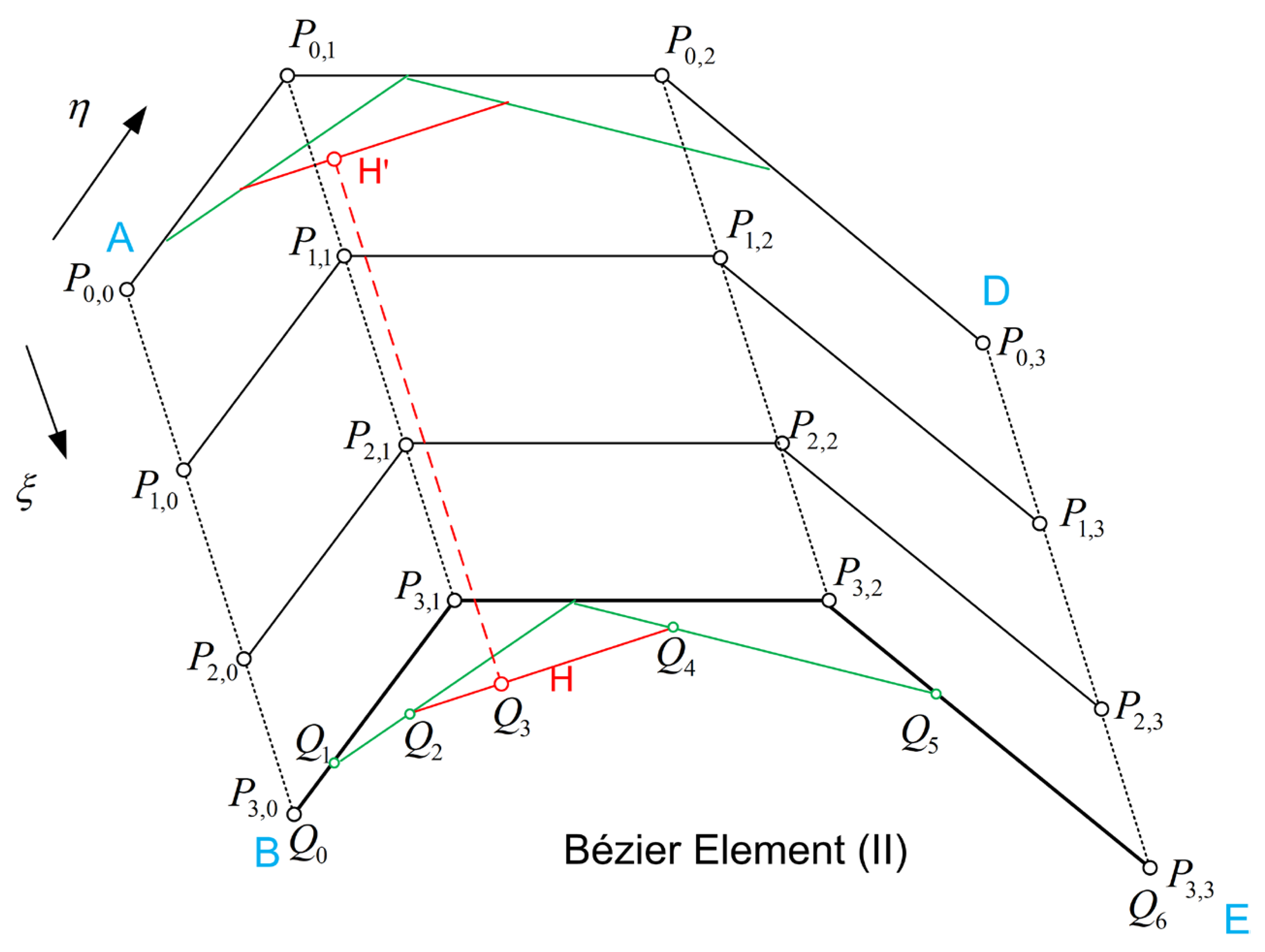
Suppressing the first subscript ‘3’ which indicates the isoline ξ = 1, let the control points along the common edge BE (see Fig. 1c) be , as shown in Figure B1. Having determined the parameter of the common point H, of known Cartesian coordinates implementing Appendix A, we set it as a new control point, and continue with the subdivision of the Bézier patch ABED by the line HH’. Then, we must determine the three control points on the left of H, and the other three control points on the right of it. Based on the same subdivision ratio , it is easy to show that these seven updated projected control points, useful for the two subdivided Bézier elements, are given by:
The above procedure is repeated to all the next three polygon lines (P0,i, P1,i, and P2,i, with i=0,1,2) shown in Figure A1.
Figure A1.
Element to be tessellated.
References
- Hughes, T.J.R.; Cottrell, J.A.; Bazilevs, Y. Isogeometric analysis: CAD, finite elements, NURBS, exact geometry and mesh refinement. Comput. Methods Appl. Mech. Eng. 2005, 194, 4135–4195. [Google Scholar] [CrossRef]
- Bazilevs, Y.; Calo, V.; Cottrell, J.; Evans, J.; Hughes, T.J.R.; Lipton, S.; Scott, M.; Sederberg, T.W. Isogeometric analysis using T-splines. Comput. Methods Appl. Mech. Eng. 2010, 199, 229–263. [Google Scholar] [CrossRef]
- Borden, M.J.; Scott, M.A.; Evans, J.A.; Hughes, T.J.R. Isogeometric finite element data structures based on Bézier extraction of NURBS. International Journal for Numerical Methods in Engineering 2011, 87, 15–47. [Google Scholar] [CrossRef]
- Scott, M.A.; Borden, M.J.; Verhoosel, C.V.; Sederberg, T.W; Hughes, T.J.R. Isogeometric finite element data structures based on Bézier extraction of T-splines. International Journal for Numerical Methods in Engineering 2011, 88, 126–156. [Google Scholar] [CrossRef]
- Cox, M.G. The numerical evaluation of B-splines. J Inst Math Its Appl 1972, 10, 134–149. [Google Scholar] [CrossRef]
- De Boor, C. On calculating with B-splines. J Approx Theory 1972, 6, 50–62. [Google Scholar] [CrossRef]
- Piegl, L.; Tiller, W. The NURBS Book. Springer, Berlin, Germany, 1997.
- Wang, Y.; Zhang, J. Control point removal algorithm for T-spline surfaces, In: M.-S. Kim and K. Shimada (Eds.): GMP 2006, LNCS 4077, Springer, pp. 385-396, 2006.
- Wang, A.; Li, L.; Wang, W.; Du, X.; Xiao, F.; Cai, Z.; Zhao, G. Linear Independence of T-Spline Blending Functions of Degree One for Isogeometric Analysis. Mathematics 2021, 9, 1346. [Google Scholar] [CrossRef]
- Lyche, T.; Mørken, K. Making the Oslo Algorithm More Efficient. SIAM Journal on Numerical Analysis 1986, 23, 663–675. [Google Scholar] [CrossRef]
- Scott, M.A. T-splines as a Design-Through-Analysis Technology, Dissertation (PhD thesis), The University of Texas at Austin, August 2011.
- Courant, R.; Hilbert, D. (1966). Methods of mathematical physics, (1st English ed., Vol. I). InterScience: New York, USA (translated and revised from the German original), 1966, pp. 300–304.
- Eisenträger, S.; Eisenträger, J.; Gravenkamp, H.; Provatidis, C.G. High order transition elements: The xNy-element concept, Part II: Dynamics. Comput. Methods Appl. Mech. Eng. 2021, 387, 114145. [Google Scholar] [CrossRef]
- Provatidis, C.G. Non-rational and rational transfinite interpolation using Bernstein polynomials. International Journal of Computational Geometry and Applications, 2022; 32, 55–89. [Google Scholar]
- Guo, M.; Wang, W.; Zhao, G.; Du, X.; Zang, R.; Yang, J. T-Splines for Isogeometric Analysis of the Large Deformation of Elastoplastic Kirchhoff–Love Shells. Appl. Sci. 2023, 13, 1709. [Google Scholar] [CrossRef]
Figure 1.
Tensor-product B-spline in (a) traditional form, (b) T-spline form after knot insertion.
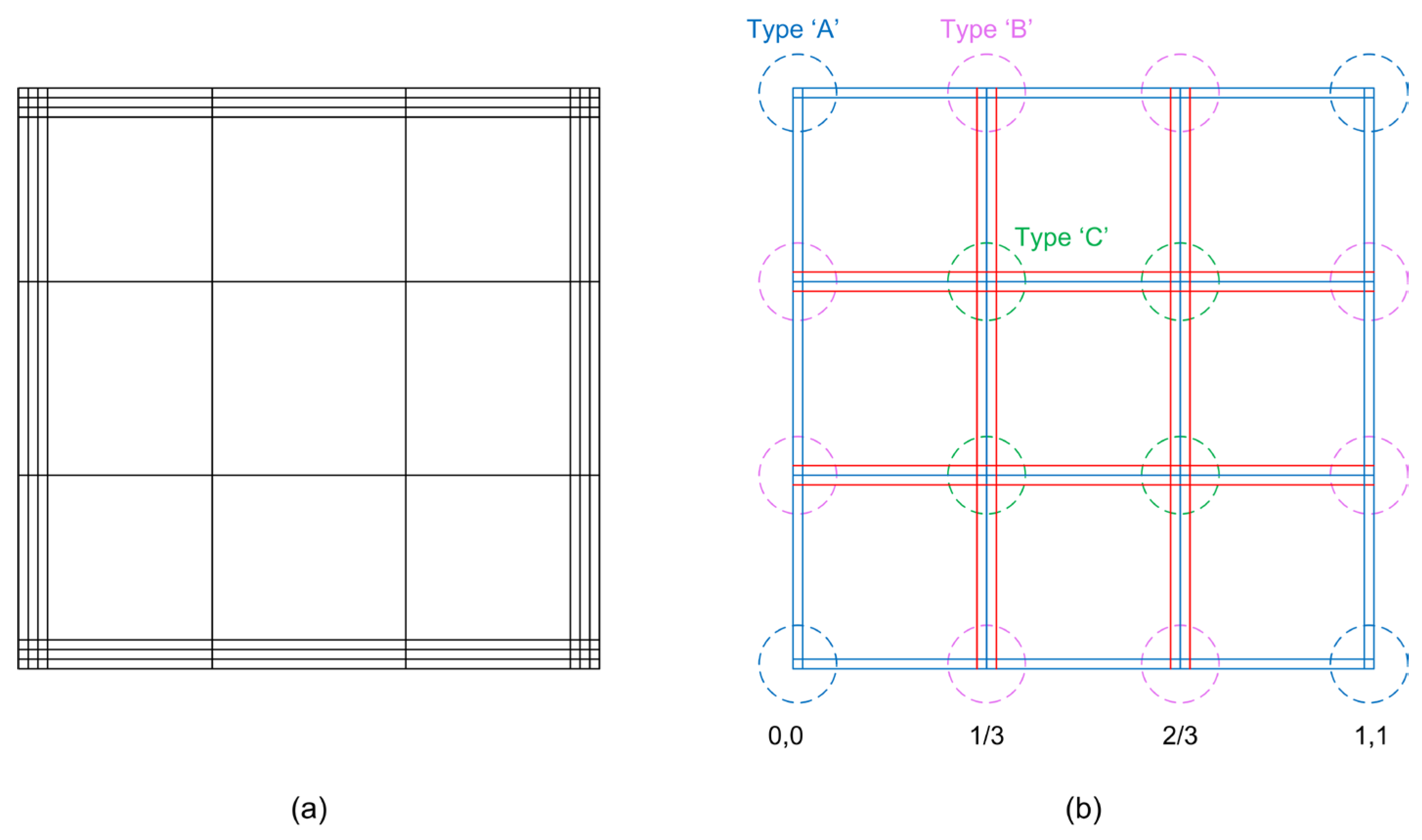
Figure 2.
Control points (a) before and (b) after knot insertion.
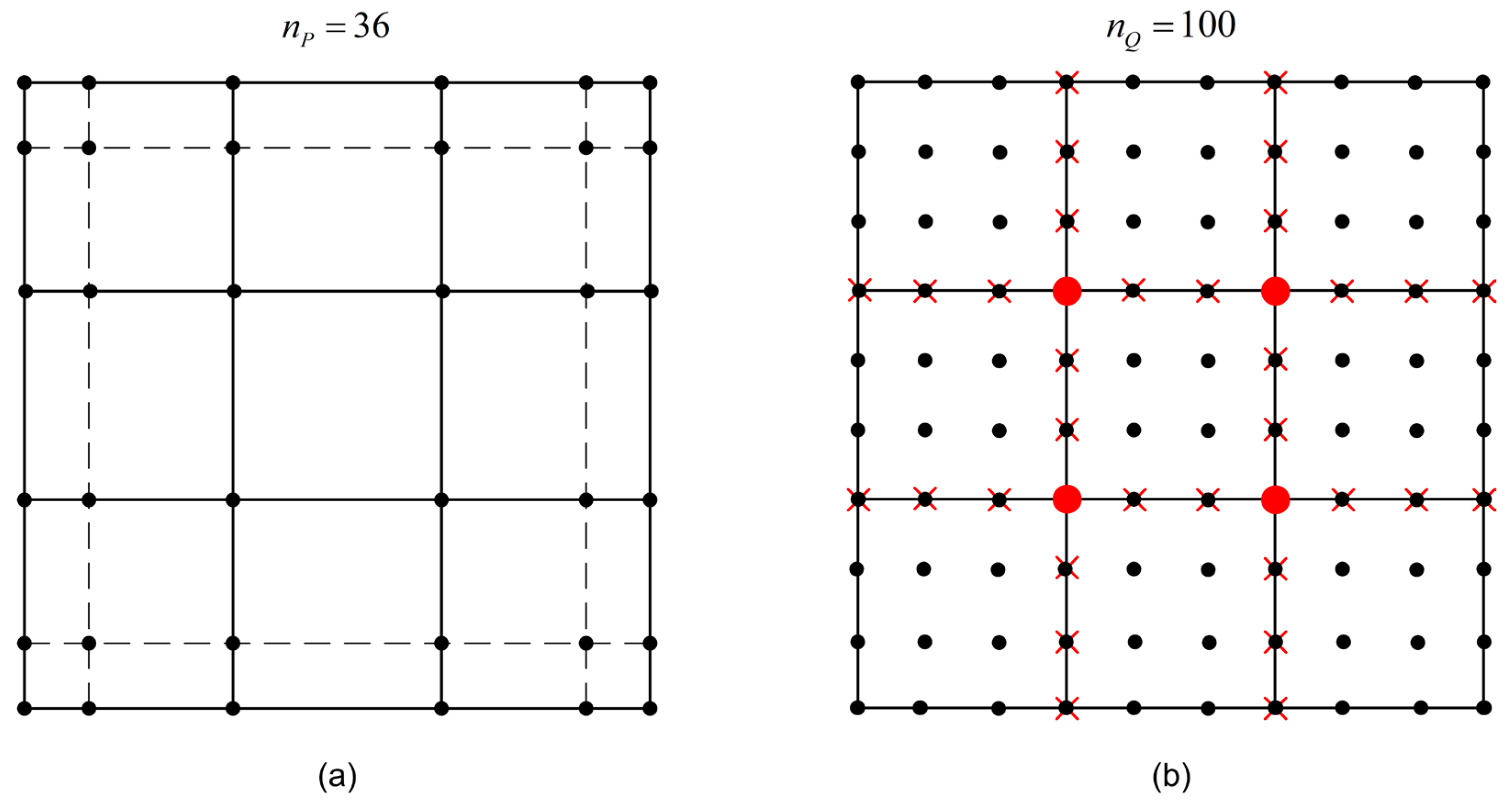
Figure 3.
Formation of Bézier elements near to reduced continuity: (a) Two sub-patches (I) and (II), (b) three incompatible elements, (c) four compatible elements.
Figure 3.
Formation of Bézier elements near to reduced continuity: (a) Two sub-patches (I) and (II), (b) three incompatible elements, (c) four compatible elements.
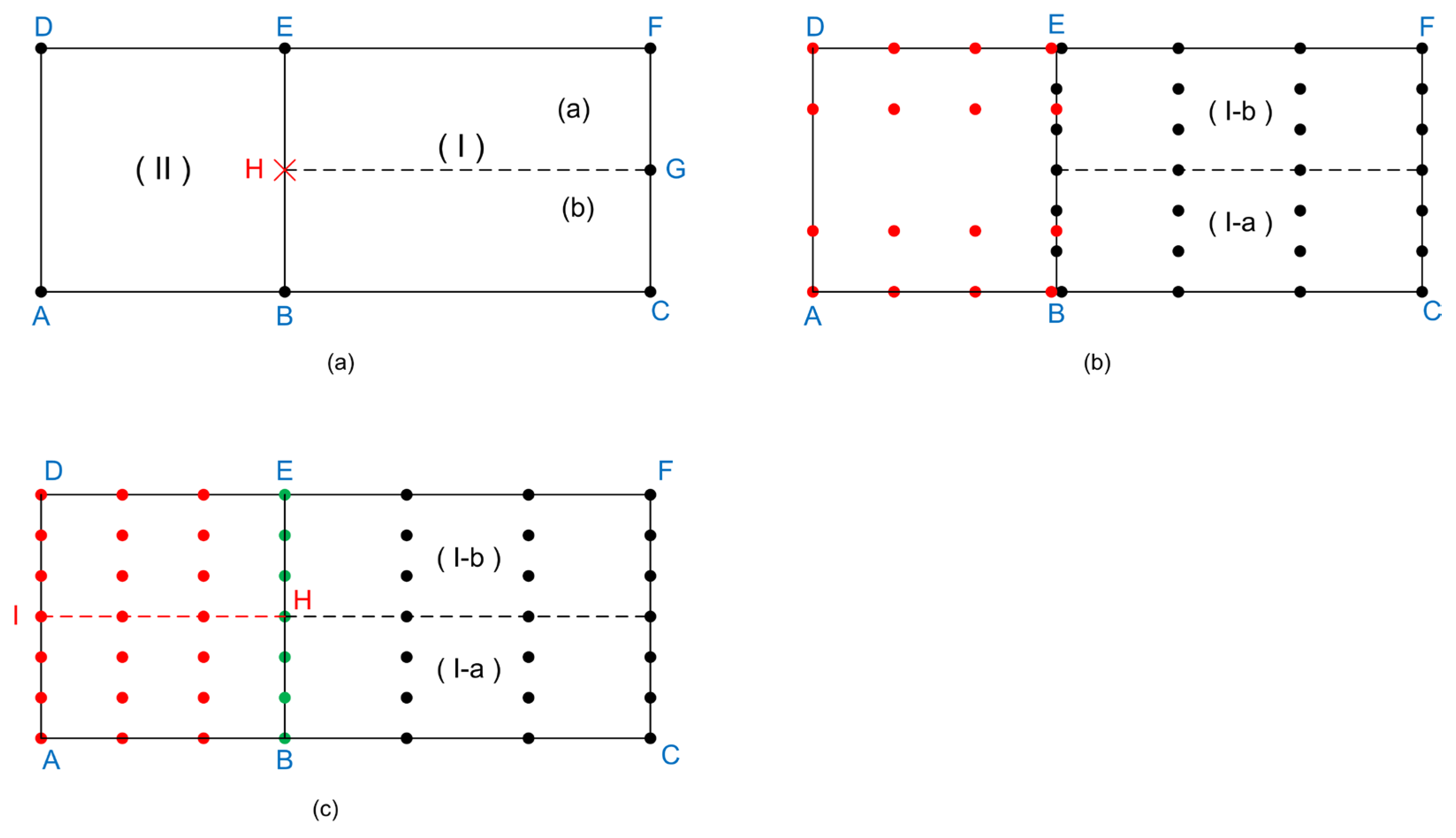
Figure 4.
Index space for Example 1 and Example 2.
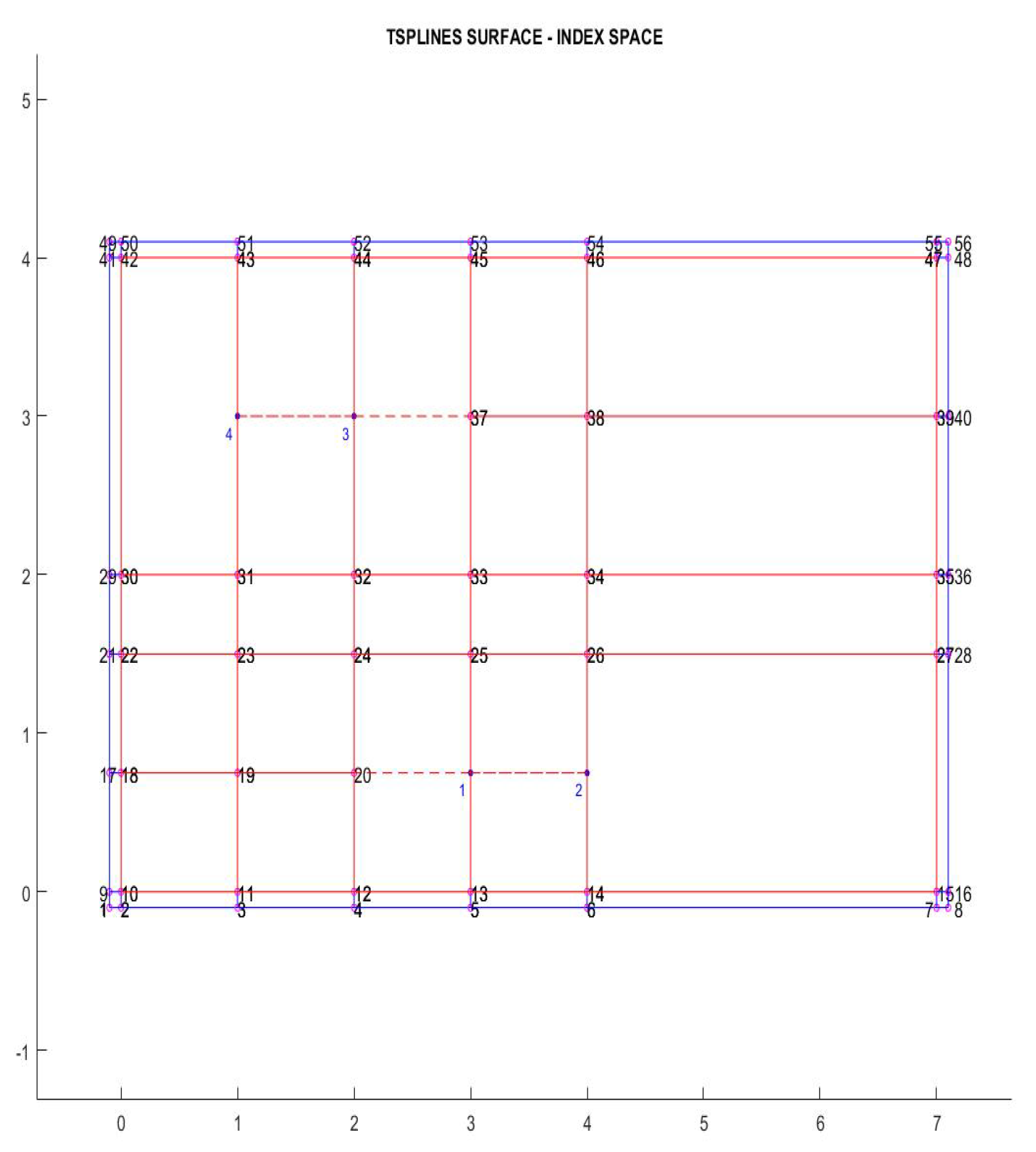
Figure 5.
Bézier elements after Bézier extraction in vertical heat flow (Example 1, MODEL-3).
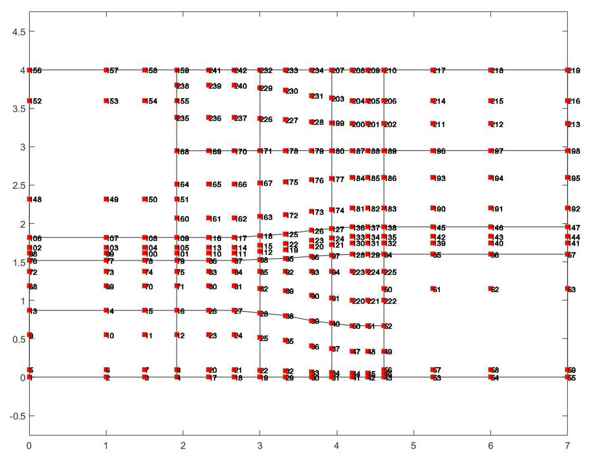
Figure 6.
Temperature distribution in vertical heat flow (Example 1).
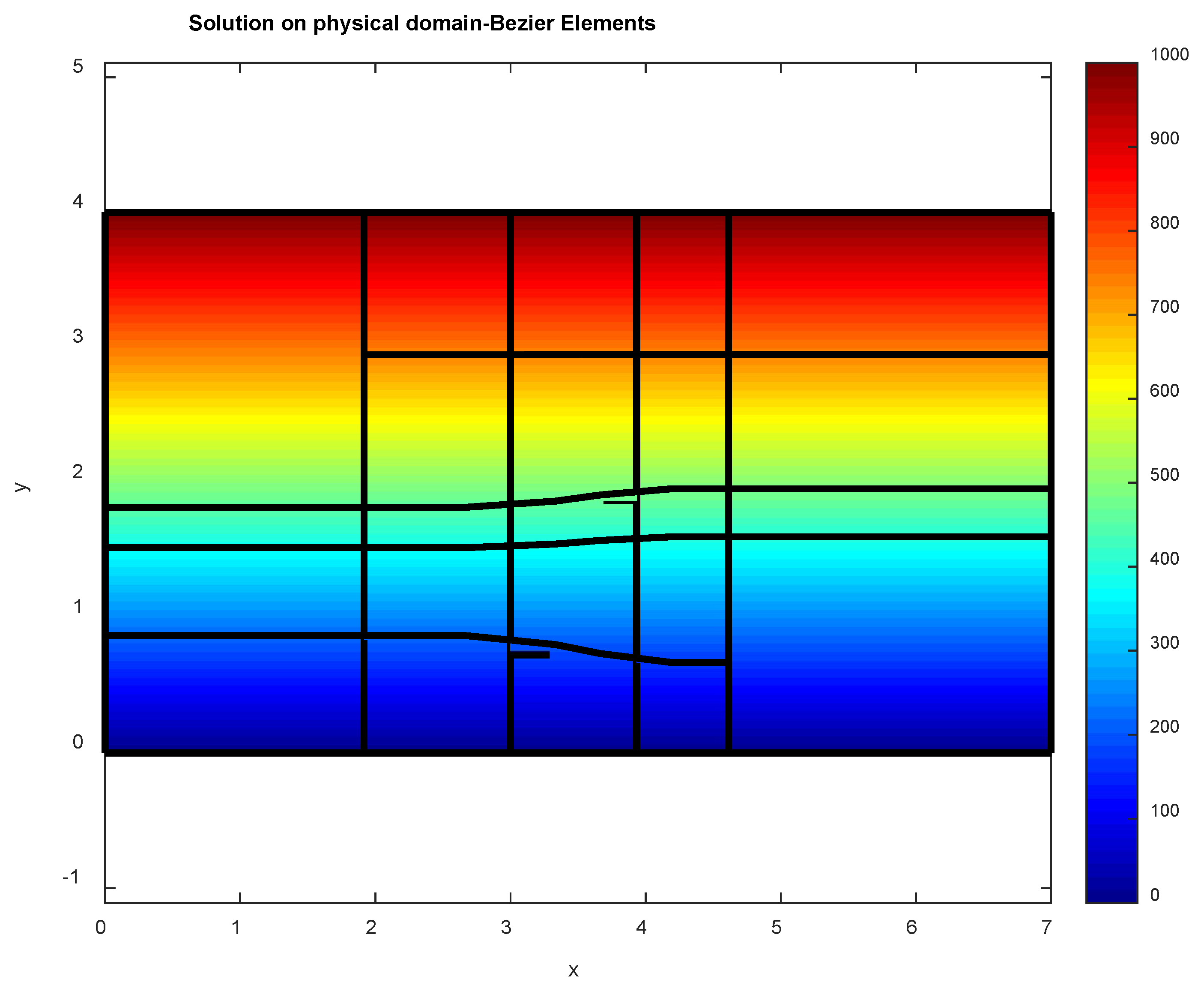
Figure 7.
Temperature distribution in MODEL-1 and MODEL-2.
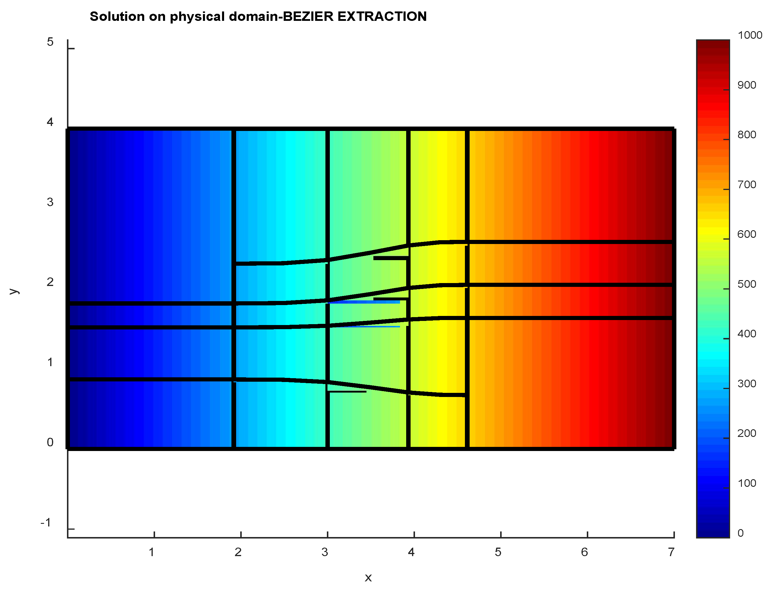
Figure 8.
Temperature distribution in MODEL-3.
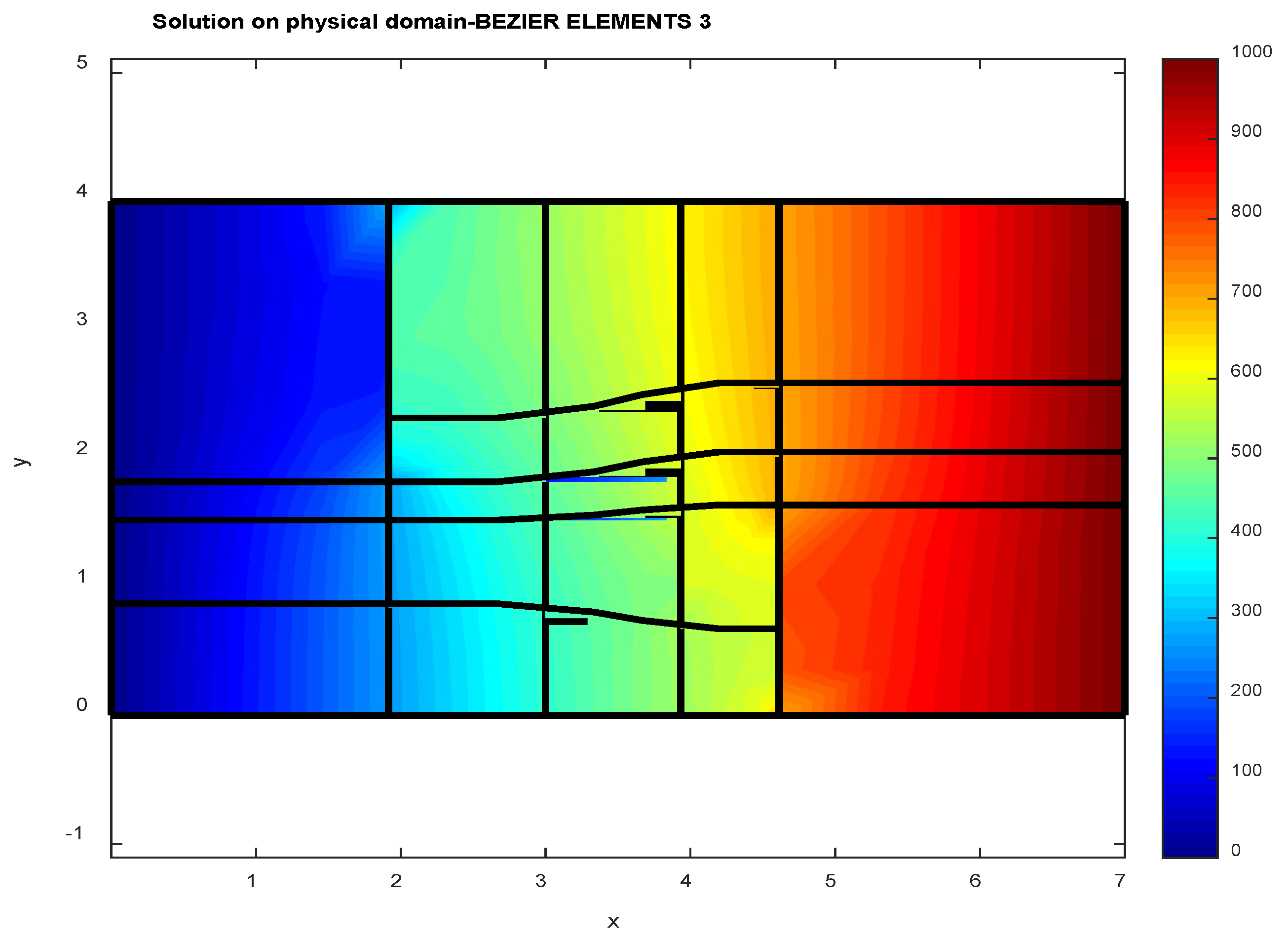
Figure 9.
Final set of Bézier elements after two subdivisions (Example 2, MODEL-4).
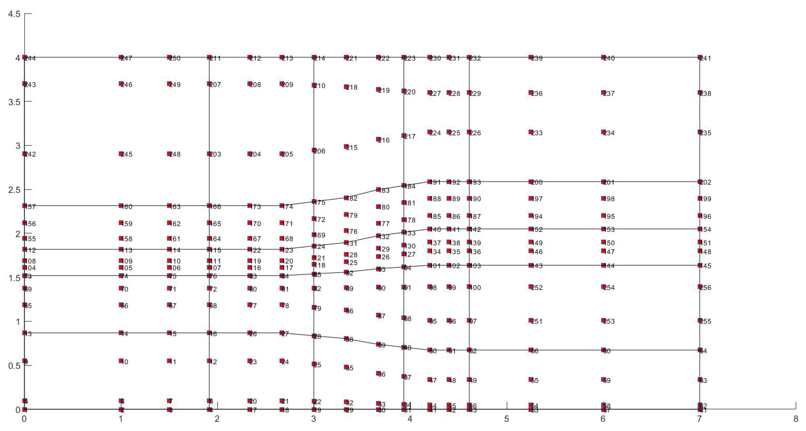
Figure 10.
Example 2: Temperature distribution using MODEL-4.
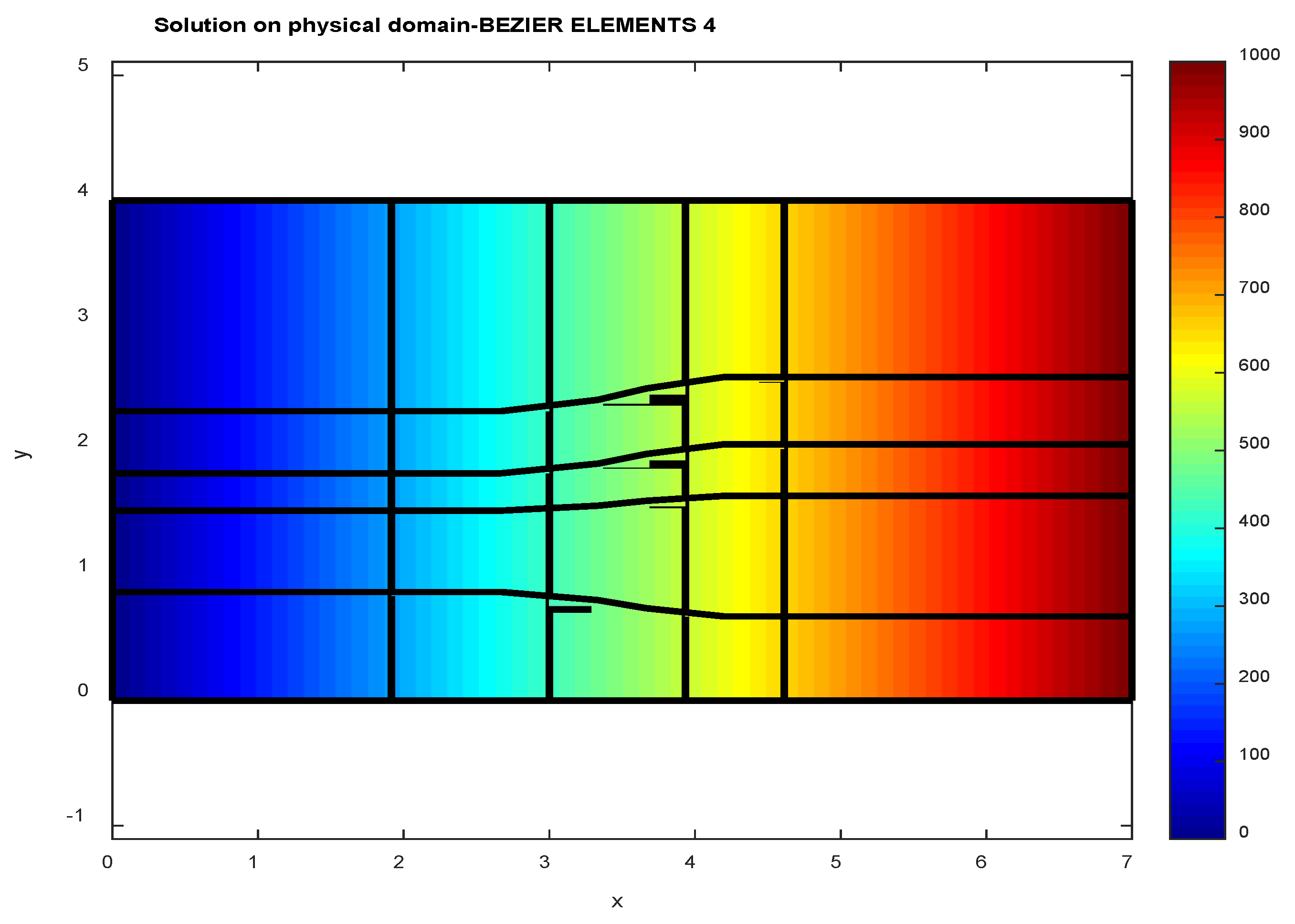
Figure 11.
Example 3 & Example 4: Index space.
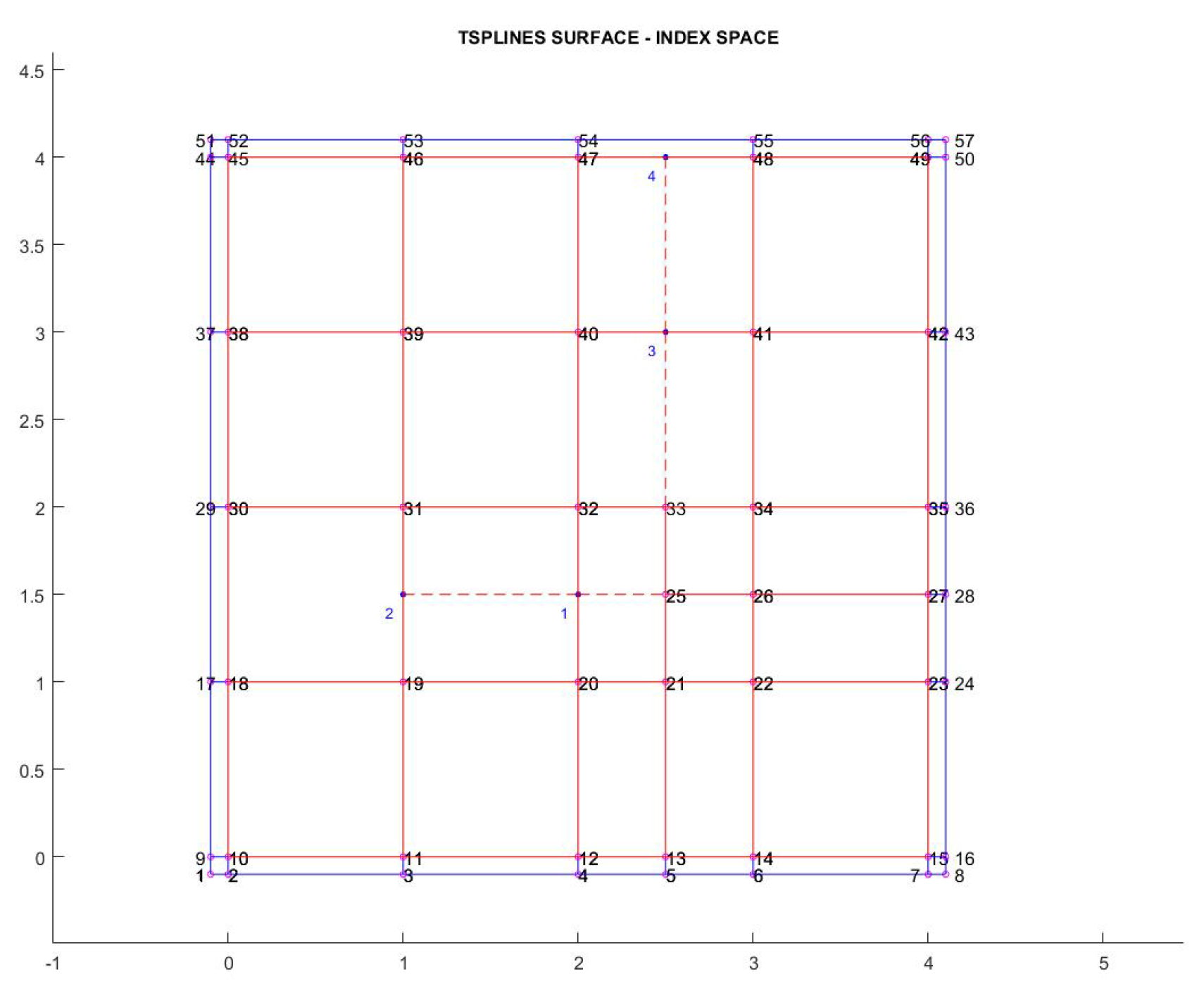
Figure 12.
Example 3: Temperature distribution (MODEL-1 & MODEL-2).
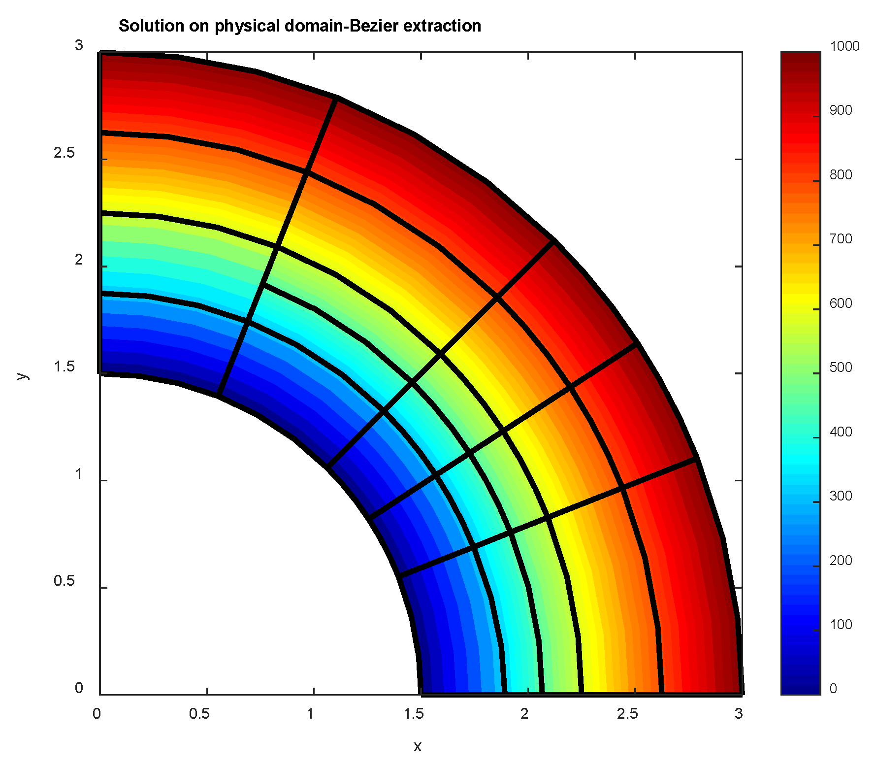
Figure 13.
Example 3 & Example 4: Incompatibility near the element of reduced continuity (MODEL-3).
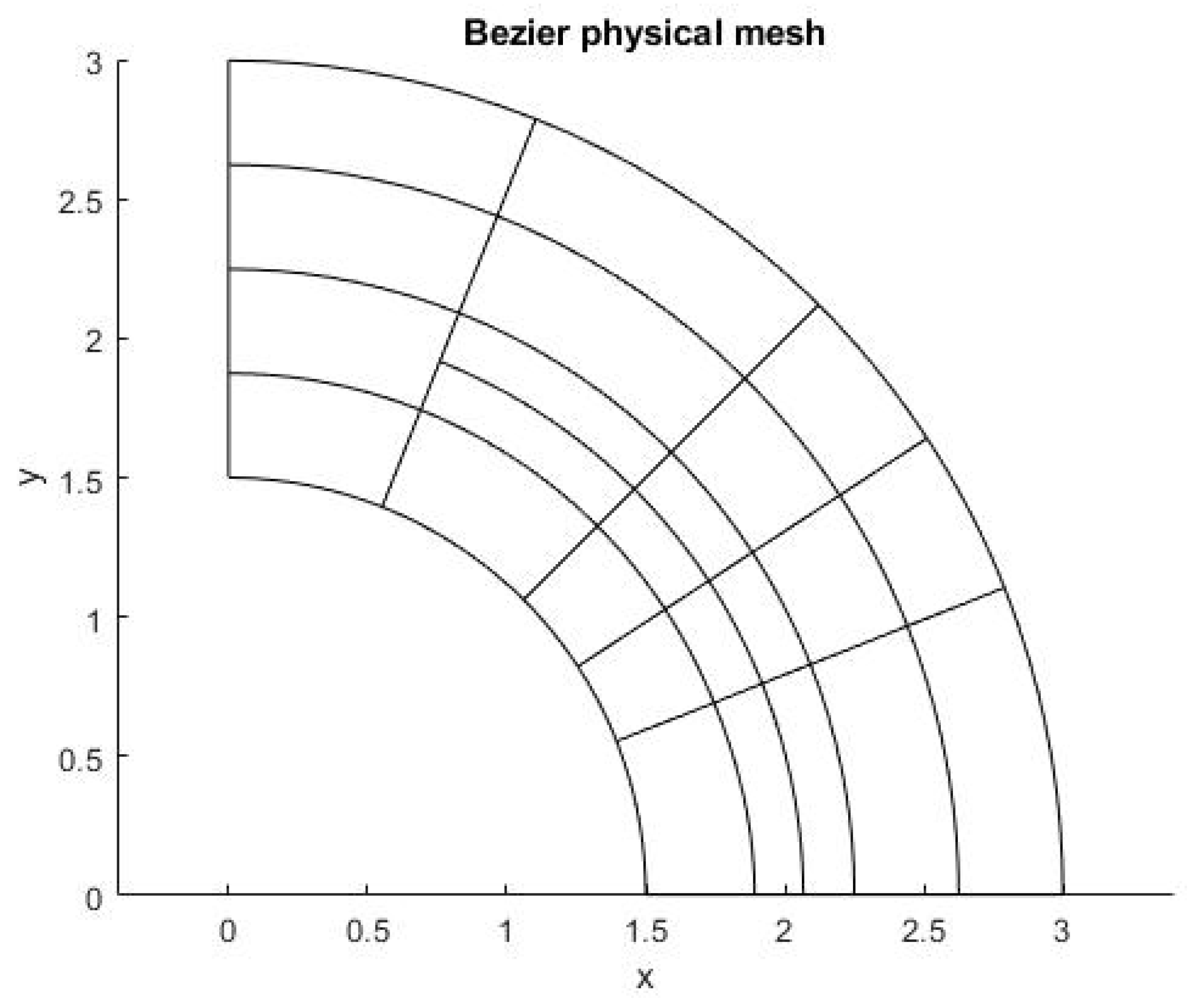
Figure 14.
Final configuration of 25 compatible Bezier elements (MODEL-4).
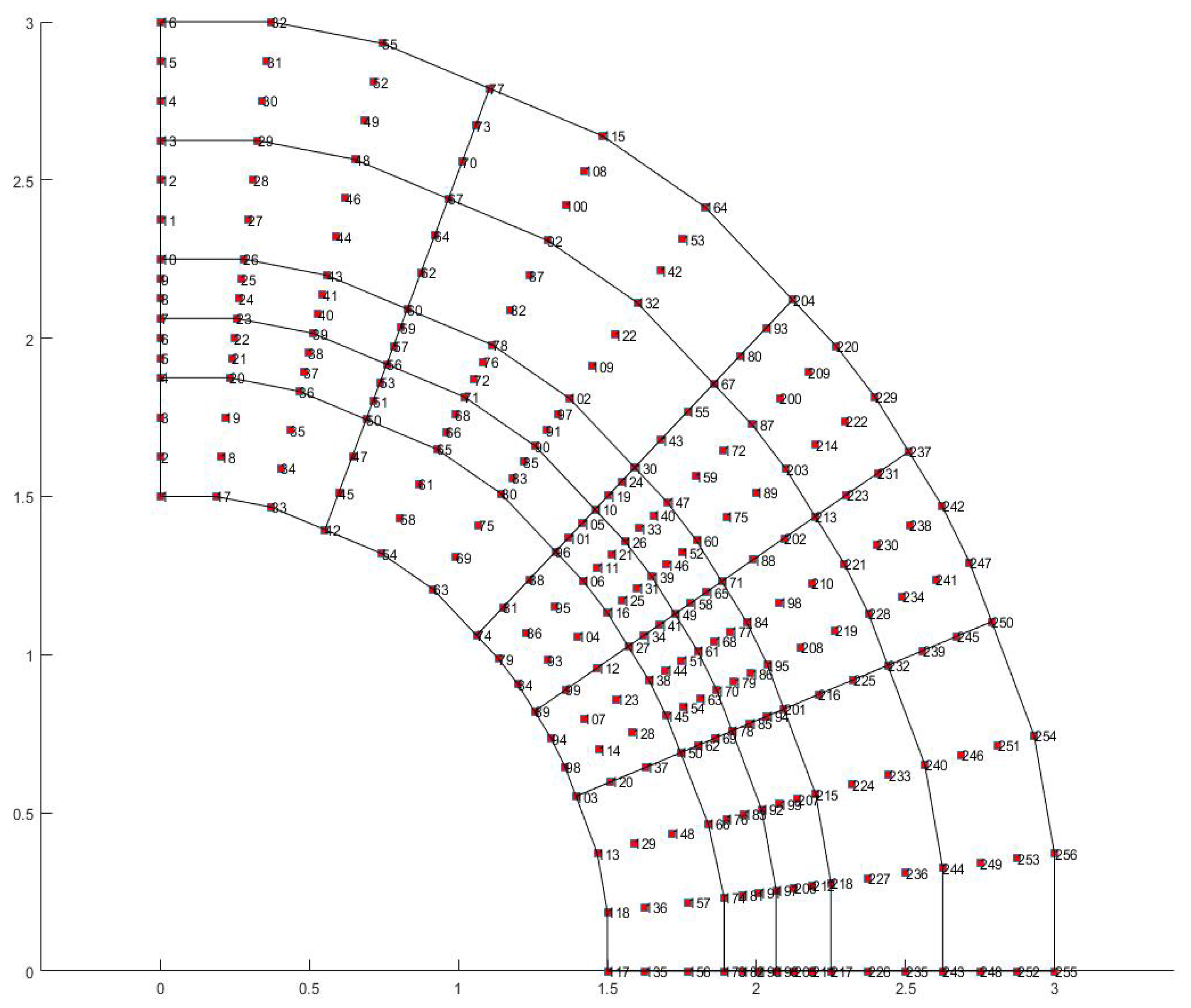
Figure 15.
Calculated eigenvalues for the rectangular acoustic cavity.
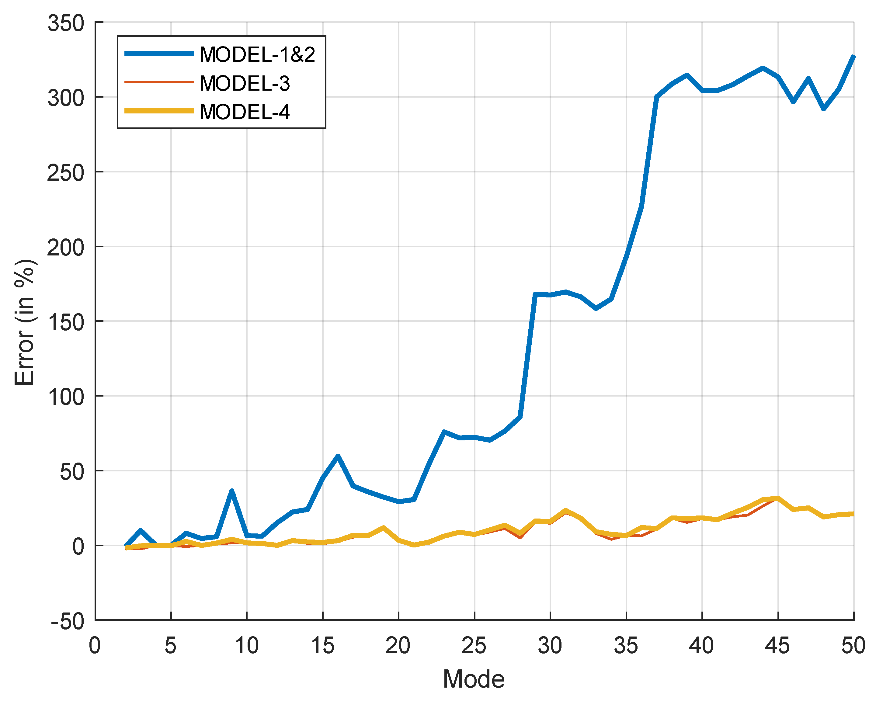

Table 1.
Estimated number of updated control points (nQ).
| Control points in MODEL-3 | |||
|---|---|---|---|
| Type A | Type B | Type C | TOTAL (nQ) |
| 4 × 4 | 14 × 6 | 16 × 9 | 244 |
Table 2.
Calculated errors for T-mesh (L2 - norm in percent).
| L2-norm in percent (%) | |||
|---|---|---|---|
|
MODEL-1 (57 DOF) |
MODEL-2 (57 DOF) |
MODEL-3 (247 DOF) |
MODEL-4 (256 DOF) |
| 0.0058 | 0.0058 | 0.0098 | 0.0016 |
Table 3.
Calculated errors for Tensor-product (L2 - norm in percent).
| L2-norm in percent (%) | |||
|---|---|---|---|
|
MODEL 1 (49 DOF) |
MODEL 2 (49 DOF) |
MODEL 3 (169 DOF) |
MODEL 4 (169 DOF) |
| 1.0785935e-03 | 1.0785935e-03 | 5.2938191e-04 | 5.2938191e-04 |
Disclaimer/Publisher’s Note: The statements, opinions and data contained in all publications are solely those of the individual author(s) and contributor(s) and not of MDPI and/or the editor(s). MDPI and/or the editor(s) disclaim responsibility for any injury to people or property resulting from any ideas, methods, instructions or products referred to in the content. |
© 2024 by the authors. Licensee MDPI, Basel, Switzerland. This article is an open access article distributed under the terms and conditions of the Creative Commons Attribution (CC BY) license (https://creativecommons.org/licenses/by/4.0/).
Copyright: This open access article is published under a Creative Commons CC BY 4.0 license, which permit the free download, distribution, and reuse, provided that the author and preprint are cited in any reuse.


