
Submitted:
28 March 2025
Posted:
28 March 2025
You are already at the latest version
Abstract
We analyzed the dynamic equilibrium process between demand and supply in the international airline market by utilizing Granger causality and Bayesian Networks (BN) based on South Korea’s aviation performance data. To examine whether the interrelationship between demand and supply varies depending on the classification of external factors, we tested for changes in causality based on reasonable segmentation of sub-market, time window, and time lag. Based on the results of the Granger causality analysis, we constructed a BN model to determine whether economic factors influence changes in the causal relationship between demand and supply, as well as to track the dynamic equilibrium path of demand and supply. The international airline market was classified into national and foreign carriers, as well as full-service carriers (FSCs) and low-cost carriers (LCCs). Time windows were set on a monthly, quarterly, and annual basis, while time lags were set with the minimum duration based on the unit of time window and the maximum duration based on data availability. Supply variables included the number of operations, available seat capacity, and load factor, whereas demand was represented by the number of revenue passengers. Our findings support the hypothesis that airline supply and demand factors in South Korea’s international airline market exhibit mutual causality. Moreover, the causality from demand to supply was found to be somewhat clearer than the reverse case. As the time window shortened, the interrelationship became more evident, and the influence of demand on supply exhibited a shorter time lag while maintaining a longer duration compared to the opposite direction. In terms of market segmentation, the relationship between supply and demand was more distinct in the LCC market compared to the FSC market and in the national carrier market compared to the foreign carrier market. The BN model incorporating economic factors confirmed that the causal relationship between airline supply and demand could appear independently of economic influences when analyzing total monthly demand. Ultimately, our study confirms the existence of a mutual causal relationship between airline supply and demand in South Korea’s international airline market. From an academic perspective, we provide insights into the dynamic equilibrium characteristics and pathways of supply and demand in the airline industry.
Keywords:
The nexus between Supply and Demand
; Airline Supply
; Air Travel Demand
; Granger Causality
; Bayesian Network
1. Introduction
In the process of forming international airline demand, we aimed to examine the mutual causal relationship between airline supply and air travel demand, segmented by sub-market, time window, and time lag. Due to the characteristics of the market—such as airline business models, the time-series nature of the data, and the presence and persistence of mutual influence—it is difficult to analyze the relationship between supply and demand from a purely aggregate perspective [1].
At the national level, international demand can be segmented into markets based on the classification of flag carriers and foreign carriers, as well as full-service carriers (FSCs) and low-cost carriers (LCCs). From a time-series perspective, demand can be divided into monthly, quarterly, and yearly units. Additionally, the complexity of the dynamic equilibrium mechanism may vary depending on how long the mutual influence between supply and demand persists [2]. We categorized South Korea’s international airline performance data into subgroups based on airline supply factors and demand, and we identified the mutual causal relationship between supply factors and demand within these given sample groups.
To test the causal relationship between airline supply and demand, we utilized Granger causality analysis, a method commonly used in economics, etc. Granger causality analysis has been applied in various fields to investigate the mutual causal relationship between supply and demand [3]. However, within our scope of review, we found no previous research in the aviation industry that has conducted a segmented analysis of the dynamic relationship between supply and demand based on real operational data, considering market segmentation, time window, and time lag. While theoretical claims suggest a mutual relationship between airline supply and demand [1], empirical verification using actual performance data has not been conducted. To validate this claim, we analyze the mutual causal relationship between airline supply and demand in South Korea’s international airline market.
Rather than examining exogenous factors, we focus on the endogenous relationship between airline supply factors and demand. Airline demand is influenced by external socioeconomic factors [4]. Accordingly, previous studies have examined how events such as the global financial crisis and COVID-19 impact the endogenous causal relationship between supply and demand [5]. However, rather than analyzing shifts in dynamic equilibrium caused by external events, we investigate how the system finds its endogenous dynamic equilibrium in the absence of external shocks. In particular, we aim to reveal the mutual causal relationship between supply and demand based on detailed analyses of market segmentation, time window, and time lag.
To verify whether the identified Granger causality represents a true causal relationship, we construct a Bayesian Network (BN) based on the statistically significant causal relationships identified. BN has been widely used in various studies as a probabilistic model to represent the interrelationships between factors [6]. Before developing sophisticated models for airline demand forecasting, we use BN to examine whether the causal relationship between supply and demand, as identified through Granger causality analysis, is influenced by exogenous economic factors. Through this approach, we aim to explore the dynamic equilibrium relationship between airline supply and demand in the context of economic factors.
In Chapter 2, we review previous studies on supply and demand in the transportation infrastructure sector, including cases where airline demand forecasting incorporates supply factors and studies that employ BN-based demand forecasting models. Chapter 3 outlines the research methodology, including Granger causality analysis and BN, as well as the data used in the study. Chapter 4 presents the results of the analysis. Finally, in the last chapter, we provide a discussion and conclusion.
2. Literature Review
Research on the demand and supply of transportation infrastructure has been continuously conducted, with several studies analyzing their interrelationship. Gnap analyzed the correlation between road and rail infrastructure in Japan and select European countries and confirmed that increased investment in transportation infrastructure is closely related to improvements in logistics performance [7]. Schwedes examined the transition from traditional supply-oriented transportation planning to demand-oriented transportation planning [8]. Using data from a study on electric vehicle charging infrastructure in Berlin, they assessed the advantages of demand-oriented planning, which moves beyond the conventional "predict and provide" approach to reflect actual user needs and demands. Agatz explored how transportation systems operate under various service models and identified new research opportunities [9]. They introduced the concept of "Transportation-Enabled Services (TRENS)" and investigated how transportation systems contribute to the provision of non-transportation services, accessibility improvements, and efficiency enhancements. Furthermore, several studies have examined the influence of external factors, such as economic conditions, on the relationship between supply and demand. Schuckmann conducted a web-based real-time Delphi study to analyze key factors affecting transportation infrastructure development by 2030 [10]. Their research evaluated the impact of factors such as increasing globalization, urbanization, public financial constraints, and population growth on transportation infrastructure demand and supply. Archetti modeled an on-demand transit system using minibuses and confirmed that integrating such systems with existing public transportation can help reduce private vehicle usage and improve transportation efficiency [11]. Doll highlighted the crucial role of public-private partnership (PPP) models in successfully implementing transportation infrastructure projects from a supply perspective and emphasized the need for sustainable financial strategies [12]. Henao analyzed the impact of sustainable transportation infrastructure investments on modal shifts, finding that continuous infrastructure investments led to decreased automobile usage and increased reliance on alternative transportation modes [13]. Their study demonstrated that transportation infrastructure investments directly influence users' mobility choices. Lundaeva developed a more precise demand forecasting model for the airline industry by utilizing historical passenger flow data [14]. Departing from conventional simple statistical forecasting methods, their study combined time series analysis using the Facebook Prophet algorithm with multiple regression analysis. The model incorporated macroeconomic indicators such as regional GDP, median per capita income, and the population sizes of departure and arrival locations. The study emphasized that airline demand forecasting should go beyond simple temporal trend analysis and account for its relationship with airline supply levels.
As an extension of research on demand and supply in the transportation market, we aim to empirically test the mutual causal relationship between airline supply and demand based on actual airline market performance and examine its characteristics.
In academic research, increasing attention is being given to airline demand forecasting models that incorporate supply factors, as opposed to studies that focus solely on demand-side factors. Abdi analyzed the impact of airline seat supply and pricing strategies on demand forecasting [15]. They developed a demand forecasting model using multiple regression analysis, incorporating seat availability and price fluctuations from the supply side. Their study nafound that seat supply and pricing strategies play a crucial role in the accuracy of demand forecasting and confirmed that demand forecasting models considering supply factors contribute to revenue maximization for airlines. Pivac examined the impact of differentiated pricing strategies in the air cargo industry on demand forecasting [16]. Their findings indicated that a demand forecasting model that simultaneously accounts for supply factors (such as cargo space availability) and pricing strategies is more accurate and effective. Lee developed a demand forecasting and price optimization model that considers substitution effects between products within the supply chain [17]. They evaluated the impact of supply adjustments on demand using Gradient Boosting Machine and Random Forest methods. Their study demonstrated that quantitatively analyzing supply-demand interactions and incorporating substitution effects and pricing strategies into demand forecasting models leads to more accurate and effective results. Birolini developed a supply-demand interaction model that integrates airline schedule design, fleet assignment, and pricing [1]. Their study quantitatively analyzed the interaction between supply and demand and emphasized the importance of an integrated decision-making model that enhances airline operational efficiency and profitability.
Unlike the majority of existing academic research, which focuses primarily on demand forecasting, our study aims to analyze the relationship between supply and demand from the perspective of mutual causality.
Bayesian Networks (BN) have been continuously utilized in demand forecasting as a methodology for effectively handling uncertainty while considering the influence of various external factors. Lee developed a Bayesian Update-based model for forecasting demand for new technologies [18]. They proposed a method to improve demand forecasting accuracy by integrating stated preferences (SP) and revealed preferences (RP), which combine consumer survey data with actual behavioral data. Bassamzadeh applied a combination of a multiscale stochastic model and a Bayesian Network (BN) to predict electricity demand in a smart grid environment [19]. Their study confirmed that BN-based models exhibit high predictive performance across different time resolutions, such as 15-minute and hourly intervals. Additionally, they demonstrated that BN models outperform conventional regression-based models by incorporating the impact of real-time electricity price fluctuations on demand patterns. Hu proposed a product demand forecasting model that integrates Bayesian Networks (BN) with a modified particle swarm optimization algorithm (MPSO) [20]. Their study introduced Bayesian inference techniques to enhance the accuracy of forecasting highly volatile demand data, outperforming traditional time series models such as ARIMA. Bhuwalka developed a hierarchical Bayesian regression model to reduce regional and industry-specific uncertainties in material demand forecasting [21]. Compared to non-hierarchical regression models, their approach reduced the uncertainty in price elasticity and income elasticity by 2.3 times and 1.6 times, respectively. Furthermore, in a 25-year forecasting scenario, uncertainty was reduced by more than tenfold. Jiangming developed a Bayesian Network (BN)-based forecasting model for predicting key material supply in uncertain environments [22]. Their study demonstrated that even in cases where historical supply data is limited, BN models can leverage existing patterns to improve supply forecasting. Compared to conventional regression-based models, BN models exhibited more stable performance in volatile environments, highlighting their potential applications in supply chain management.
As a means of analyzing how the mutual causality between supply and demand factors interacts with economic factors, we employ the BN methodology, whose validity has been demonstrated in previous research.
3. Methodology
3.1. Overall Research Landscape
In this study, we analyze the dynamic equilibrium process between demand factors and airline supply factors in the aviation market by conducting a Granger causality analysis and constructing Bayesian Networks (BN) based on past international airline market performance and economic indicators in South Korea. The supply variables considered are the number of operations, available seat capacity, and load factor, while the demand variable is the number of revenue passengers. The international airline market is segmented based on market segmentation, time window, and time lag. The market is classified into full-service carriers (FSCs) and low-cost carriers (LCCs), as well as foreign and flag carriers. The time window is divided into monthly, quarterly, and annual units, while the time lag is set with the minimum unit being the time window itself and the maximum unit determined based on data constraints.
Through Granger causality analysis, we test whether there is a time-lagged mutual relationship between supply and demand factors. Additionally, we construct a Bayesian Network from a total monthly demand perspective that incorporates economic factors affecting demand, as suggested in previous research [23]. This allows us to examine changes in the interrelationship between supply and demand and to provide illustrative insights into the dynamic equilibrium pathways when economic factors are introduced.
In this study, the time lag is set as follows: for monthly data, from 1 month to 36 months; for quarterly data, from 1 quarter to 12 quarters; and for annual data, from 1 year to 10 years. The time-lag settings for each data segmentation are presented in the following table, reflecting seasonal patterns and periodicity. Particularly, the Granger causality analysis conducted in this study enables us to examine how past data influences future values, allowing for the establishment of diverse scenario-based time-lag settings. Table 1 presents the data segmentation categorized by time, while Table 2 delineates the configuration values for the classification of variable codes based on data types.
3.2. Granger Causality Analysis
Granger causality is a statistical method used to test whether one variable provides significant information for predicting the future values of another variable. In other words, if the past values of X have explanatory power for the present or future values of Y, then X is said to Granger-cause Y [24]. To test for Granger causality, two regression equations must be established [25].
(1) Restricted Model
(2) Unrestricted Model
: Dependent variable at time t
: Independent variable at time t
: Number of lags
: Regression coefficient
: Error term
By comparing the restricted model and the full model, we test whether the inclusion of X significantly improves the predictive power for Y. To conduct the Granger causality test, the F-statistic is used to establish the null and alternative hypotheses [25].
That is, the past values of X do not affect the future values of Y.
(3) Calculation of the F-statistic
In the case of Granger causality analysis, the method for calculating the F-statistic using the sum of squared residuals of the restricted model and the full model is as follows [25].
: Residual Sum of Squares of the restricted model
: Residual Sum of Squares of the full model
: Sample size
: Number of lags
If the calculated F-value is greater than the critical value at a given significance level, the null hypothesis is rejected, and X is determined to be the Granger cause of Y [26].
3.3. Bayesian Network Analysis
A Bayesian Network (BN) is a probabilistic graphical model based on conditional independence among random variables. It is widely used for probabilistic decision-making, causal analysis, and predictive modeling. A Bayesian Network is represented as a Directed Acyclic Graph (DAG), where each node represents a random variable, and each edge denotes a conditional dependency between variables. A Bayesian Network consists of nodes that represent random variables, edges that indicate conditional dependencies between nodes, and conditional probability distributions, which define the probability distribution of a dependent node given the values of its parent nodes. In a Bayesian Network, relationships between variables are calculated using Bayes’ theorem, and the formula is expressed as follows [27].
: The probability of event A occurring given that event B has occurred (Posterior Probability)
: The probability of event B occurring given that event A has occurred (Likelihood)
: The prior probability of event A (Prior Probability)
: The total probability of event B (Marginal Probability)
In a Bayesian Network, a Conditional Probability Table (CPT) is generated for each node to quantify the relationships between variables. For example, if two variables X and Y exist, and Y is assumed to be the parent node of X, the following CPT can be set. Inference in a Bayesian Network is the process of updating the probability of a specific variable based on observed data. It is classified into Exact Inference, which calculates accurate probabilities using Variable Elimination or Dynamic Programming, and Approximate Inference, which estimates probabilities using sampling-based algorithms. Additionally, to evaluate the performance of a Bayesian Network model, Log-Likelihood (LL), Kullback-Leibler Divergence (KL-divergence), and Structural Learning Accuracy can generally be used as evaluation metrics [28].
4. Result
4.1. Basic Analysis Results
We divided the basic statistics of the utilized data into monthly, quarterly, and yearly time series for basic analysis. Additionally, we compared the average growth rate, range, and trends in the number of passengers per unit of supply. The summarized basic statistical results for each dataset are provided in the Appendix A.

Table 3.
Basic Analysis Results by Utilized Data (Average Growth Rate, Count, Standard Deviation).
| Type | Average Growth Rate(%) | Count | Standard Deviation | ||||||
|---|---|---|---|---|---|---|---|---|---|
| Month | Quarter | Year | Month | Quarter | Year | Month | Quarter | Year | |
| Total_Pax | 2.593 | 10.215 | 26.414 | 132 | 44 | 32 | 2,542,443 | 7,519,740 | 24,023,380 |
| Flag_Pax | 2.677 | 10.571 | 30.197 | 132 | 44 | 32 | 1,725,968 | 5,107,447 | 16,302,388 |
| FA_Pax | 2.559 | 10.018 | 21.107 | 132 | 44 | 32 | 829,698 | 2,450,270 | 7,804,372 |
| FSC_Pax | 1.770 | 7.027 | 19.506 | 132 | 44 | 32 | 1,035,209 | 3,076,083 | 9,675,428 |
| LCC_Pax | 6.500 | 27.860 | 795.323 | 132 | 44 | 17 | 836,870 | 2,474,587 | 9,715,016 |
| Total_S | 1.845 | 6.949 | 14.178 | 132 | 44 | 32 | 2,930,379 | 8,689,327 | 27,934,005 |
| Flag_S | 1.948 | 7.049 | 15.789 | 132 | 44 | 32 | 1,976,027 | 5,858,291 | 18,997,255 |
| FA_S | 1.754 | 7.010 | 11.886 | 132 | 44 | 32 | 967,740 | 2,868,956 | 9,056,260 |
| FSC_S | 1.087 | 3.910 | 9.375 | 132 | 44 | 32 | 1,199,578 | 3,574,850 | 11,576,203 |
| LCC_S | 5.713 | 22.666 | 864.268 | 132 | 44 | 17 | 970,195 | 2,873,882 | 11,295,685 |
| Total_LF | 0.514 | 1.757 | 5.538 | 132 | 44 | 32 | 18.231 | 18.054 | 10.674 |
| Flag_LF | 0.531 | 1.100 | 4.682 | 132 | 44 | 32 | 16.419 | 16.065 | 10.243 |
| FA_LF | 0.592 | 1.956 | 5.885 | 132 | 44 | 32 | 18.427 | 18.259 | 10.828 |
| FSC_LF | 0.855 | 1.364 | 3.427 | 132 | 44 | 32 | 15.430 | 15.090 | 8.154 |
| LCC_LF | 0.574 | 0.860 | 7.369 | 132 | 44 | 17 | 17.823 | 17.377 | 13.300 |
The average growth rate showed an increasing trend from monthly to yearly data, with the LCC group exhibiting the highest growth rate and the FSC group showing the lowest. Regarding standard deviation, foreign airlines (FA) recorded the lowest value, which suggests potential implications for data consistency and pattern analysis. In the market-specific trends of monthly data, the differences between FSC and LCC were more pronounced compared to the total (overall market). For FSCs, which entered an existing market, the fluctuations in supply variables and demand trends were relatively large. In contrast, LCCs, as new market entrants, exhibited a steep upward trend, with supply variables following a pattern similar to demand, more so than in other market segments.
4.2. Overview of Causality Analysis Results
The Granger causality analysis was conducted on the combination groups formed based on variables, time windows, and time lags. The results show that evidence of a mutual causal relationship between airline supply and air travel demand was found more than four times as often as cases where no such evidence was identified. As shown in Figure 1, out of 90 total combinations, only 15 cases (17%) did not provide evidence of causality. Regarding the direction of causality between supply and demand, it was more difficult to find evidence that supply causes demand than the reverse. Among the cases analyzed, there were 5 instances where no evidence was found that demand causes supply, while there were 10 instances where no evidence was found that supply causes demand. In the South Korean market examined in this study, the hypothesis that a mutual causal relationship exists between supply and demand is supported, with demand more frequently acting as a cause of supply than the other way around.
From a time window perspective, all monthly cases showed mutual causality, except for the combination of low-cost carriers (LCC) passengers and load factor. Conversely, cases where causality was not supported were most frequently observed in the yearly time window, indicating that larger time windows make it more difficult to detect causality. Furthermore, in all combinations of supply variables set as frequency, available seats, and load factor, there were no cases where demand and supply lacked causality. This strongly supports the hypothesis that a mutual causal relationship exists between supply and demand.
Time lag and complexity varied depending on the time window unit and the causality direction between supply and demand (Appendix A, Table A1). The impact of demand on supply lasted for both short and extended durations in more combinations than the impact of supply on demand. Among the combinations where causality was observed, there were no cases where supply started influencing demand before the reverse was observed. However, in some cases, the effect of supply on demand persisted longer. In certain cases, the impact might extend beyond the predefined time lag limit due to data constraints. This phenomenon further supports the hypothesis that the influence of demand on supply is stronger than that of supply on demand.
From a market segmentation perspective, causality was less frequently observed in FSCs compared to LCCs and in foreign airlines compared to flag carriers. Regarding the impact of demand on supply, causality was observed in all possible cases for LCCs and flag airlines. In contrast, cases where causality was not observed for supply impacting demand were found primarily in FSCs and foreign airlines, except for LCC load factor & LCC demand and flag airline load factor & flag airline demand.
Table 4.
Cases Where No Evidence of Causality Was Found (Based on Granger Causality Analysis).
| Causality | Demand Variable | Supply Variable | Time Window |
|---|---|---|---|
| Demand Causes Supply | Total Passenger | Total Available Seats | Year |
| FSC Passenger | FSC Frequency | Quarter | |
| FSC Passenger | FSC Available Seats | Year | |
| Foreign Airrline Passenger | Foreign Airline Frequency | Quarter | |
| Foreign Airrline Passenger | Foreign Airline Available Seats | Year | |
| Supply Causes Demand | Total_Passenger | Total Load Factorr | Year |
| Total_Passenger | Total Available Seats | Year | |
| FSC Passenger | FSC Frequency | Quarter | |
| FSC Passenger | FSC Load Factor | Year | |
| FSC Passenger | FSC Available Seats | Quarter, Year | |
| LCC Passenger | LCC Load Factor | Month, Year | |
| Flag Airline Passengerr | Flag Airline Load Factor | Year | |
| Foreign Airrline Passenger | Foreign Airline Frequency | Quarter | |
| Foreign Airrline Passenger | Foreign Airline Load Factor | Year | |
| Foreign Airrline Passenger | Foreign Airline Available Seats | Year |
4.3. Causality Analysis Results by Market
The market-specific causality analysis examines the time lag in the relationship between supply and demand by analyzing the minimum and maximum values of the time lag for each supply variable. Since using the average may distort the interpretation of the time lag in the supply-demand relationship, we apply the min-min and max-max methodology, which selects one of the three variables based on the minimum of the minimum values and the maximum of the maximum values.
4.3.1. FSC vs. LCC
Based on the monthly time window, FSC supply was found to influence demand from 3 months to 36 months prior (the study's time limit), while total demand was affected by supply from 6 months to 36 months prior. In all other cases, supply and demand continuously influenced each other from 1 month to 36 months prior. This suggests that, on a monthly basis, demand responds to supply with a greater lag in FSC compared to LCC.
In the quarterly time window, the time lag patterns for FSC and LCC supply and demand were found to be different. For FSCs, demand influenced supply from 1 quarter to 8 quarters prior, while supply influenced demand from 1 quarter to 12 quarters prior. This suggests that supply has a longer-lasting effect on demand. In contrast, for LCCs, the opposite pattern was observed: demand influenced supply from 1 quarter to 12 quarters prior, while supply influenced demand from 1 quarter to 8 quarters prior. These findings indicate that the causal relationship between supply and demand differs between FSCs and LCCs when viewed on a quarterly basis.
For the yearly time window, FSCs showed a mutual influence between supply and demand from 2 years to 5 years prior. In contrast, LCC demand influenced supply from 1 year to 3 years prior, while supply had a 3-year lag before influencing demand. This suggests that, even on a yearly basis, the mutual causality between supply and demand differs between FSCs and LCCs, supporting the hypothesis that the two market segments exhibit distinct causal patterns.
Table 5.
Comparison of FSC and LCC Time Lag (Based on Minimum and Maximum Values).
| Variable | Time Window | Causality | Time lag | ||
|---|---|---|---|---|---|
| Demand | Supply | Min | Max | ||
| Total_P | Min-Max | Month | Demand Causes Supply | 1 | 36 |
| Total_P | Min-Max | Month | Supply Causes Demand | 6 | 36 |
| FSC_P | Min-Max | Month | Demand Causes Supply | 1 | 36 |
| FSC_P | Min-Max | Month | Supply Causes Demand | 3 | 36 |
| LCC_P | Min-Max | Month | Demand Causes Supply | 1 | 36 |
| LCC_P | Min-Max | Month | Supply Causes Demand | 1 | 36 |
| Total_P | Min-Max | Quarter | Demand Causes Supply | 1 | 8 |
| Total_P | Min-Max | Quarter | Supply Causes Demand | 1 | 6 |
| FSC_P | Min-Max | Quarter | Demand Causes Supply | 1 | 8 |
| FSC_P | Min-Max | Quarter | Supply Causes Demand | 1 | 12 |
| LCC_P | Min-Max | Quarter | Demand Causes Supply | 1 | 12 |
| LCC_P | Min-Max | Quarter | Supply Causes Demand | 1 | 8 |
| Total_P | Min-Max | Year | Demand Causes Supply | 2 | 5 |
| Total_P | Min-Max | Year | Supply Causes Demand | 2 | 3 |
| FSC_P | Min-Max | Year | Demand Causes Supply | 2 | 5 |
| FSC_P | Min-Max | Year | Supply Causes Demand | 2 | 5 |
| LCC_P | Min-Max | Year | Demand Causes Supply | 1 | 3 |
| LCC_P | Min-Max | Year | Supply Causes Demand | 3 | 3 |
4.3.2. NA vs. FA
Based on the monthly time window, supply and demand were found to have a mutual causal relationship from 1 month to 36 months prior, regardless of whether the airline was a national carrier or a foreign airline. However, in terms of total demand, supply influenced demand from 6 months to 36 months prior, suggesting that the combined analysis of national and foreign carriers produces different interpretations. This phenomenon is attributed to the significant performance differences between national and foreign carriers in terms of supply and demand.
For the quarterly time window, national and foreign carriers generally exhibited mutual influence from 1 quarter to 12 quarters prior, except in the case of flag carriers, where supply influenced demand only from 1 quarter to 6 quarters prior. However, total demand showed slightly different results, similar to those observed in the monthly time window analysis. In terms of demand's influence on supply, total demand followed a pattern similar to flag carriers, where past performance from 1 quarter to 6 quarters prior affected current supply. However, in terms of supply's influence on demand, the time lag was found to be from 1 quarter to 8 quarters prior, exhibiting a different pattern from both national and foreign carriers.
For the yearly time window, flag carriers showed mutual causality between supply and demand from 2 years to 5 years prior. In contrast, foreign carriers exhibited a pattern where demand influenced supply from 1 year to 3 years prior, while supply influenced demand with a lag of 2 to 3 years. In terms of total demand, demand's influence on supply followed the pattern of flag carriers, while supply's influence on demand followed the pattern of foreign carriers. The yearly analysis results suggest that the mutual relationship between supply and demand is significantly influenced by whether an airline is a national or foreign carrier.
Table 6.
Comparison of Time Lag Between National and Foreign Carriers (Based on Minimum and Maximum Values).
Table 6.
Comparison of Time Lag Between National and Foreign Carriers (Based on Minimum and Maximum Values).
| Variable | Time Window | Causality | Time lag | ||
|---|---|---|---|---|---|
| Demand | Supply | Min | Max | ||
| Total_P | Min-Max | Month | Demand Causes Supply | 1 | 36 |
| Total_P | Min-Max | Month | Supply Causes Demand | 6 | 36 |
| Flag_P | Min-Max | Month | Demand Causes Supply | 1 | 36 |
| Flag_P | Min-Max | Month | Supply Causes Demand | 1 | 36 |
| FA_P | Min-Max | Month | Demand Causes Supply | 1 | 36 |
| FA_P | Min-Max | Month | Supply Causes Demand | 1 | 36 |
| Total_P | Min-Max | Quarter | Demand Causes Supply | 1 | 8 |
| Total_P | Min-Max | Quarter | Supply Causes Demand | 1 | 6 |
| Flag_P | Min-Max | Quarter | Demand Causes Supply | 1 | 12 |
| Flag_P | Min-Max | Quarter | Supply Causes Demand | 1 | 6 |
| FA_P | Min-Max | Quarter | Demand Causes Supply | 1 | 12 |
| FA_P | Min-Max | Quarter | Supply Causes Demand | 1 | 12 |
| Total_P | Min-Max | Year | Demand Causes Supply | 2 | 5 |
| Total_P | Min-Max | Year | Supply Causes Demand | 2 | 3 |
| Flag_P | Min-Max | Year | Demand Causes Supply | 2 | 5 |
| Flag_P | Min-Max | Year | Supply Causes Demand | 2 | 5 |
| FA_P | Min-Max | Year | Demand Causes Supply | 1 | 3 |
| FA_P | Min-Max | Year | Supply Causes Demand | 2 | 3 |
4.4. Bayesian Network Analysis Results
We represented the relationship between demand and supply concerning the total monthly demand and economic indicators using a Bayesian Network. The Bayesian Network was utilized to integrate economic factors and the demand-supply relationship derived from Granger causality. Socioeconomic indicators were incorporated into the model based on the findings of a previous study (Song, K.H. et al., 2023). The model included the number of flights and available seat capacity from one month prior, the number of flights six months later, the available seat capacity twelve months later, and the current total international demand. A static model was constructed to examine whether the independent relationship between demand and supply changes when economic factors are introduced and to conceptually observe the interconnection with economic factors. To align with the study's objectives, the continuous mutual influence between demand and supply was excluded, as was the Load Factor derived from their interaction.
The results of the Bayesian Network construction are shown in Figure 3, with detailed parameters presented in Appendix A Table A2. The impact of economic indicators on demand is reflected in two aspects: economic conditions and exchange rates. The findings confirm previous research [23], which suggested that monthly air travel demand, as a short-term demand indicator, can be influenced by exchange rates. The direction of changes in demand and supply derived from the Granger causality analysis was found to remain consistent regardless of the presence of economic indicators. However, the model suggested that the supply indicator from one month prior affects economic indicators, despite the lack of a clear direct relationship. This appears to represent a hidden relationship rather than a true causal effect, where the supply indicator acts as a proxy reflecting the impact of economic indicators from one or more months earlier, which in turn influences current economic indicators.
The Bayesian Network analysis revealed additional relationships not identified in the Granger causality analysis. Specifically, the number of flights was found to influence the available seat capacity, and both supply factors were found to impact demand. This result supports the logical assumption that an increase in the number of flights leads to an increase in available seat capacity. Additionally, the fact that both factors simultaneously affect demand suggests that variations in fleet composition, which influence seat capacity but are not directly reflected in flight frequency, also play a role in shaping demand. The previously mentioned relationships also hold in patterns where current demand influences future supply. This indicates that airlines adjust their future flight frequencies and seat capacities based on current demand trends.
5. Discussion & Conclusion
We have found that considering both cross-sectional and time-series market segmentation is crucial in studying the international airline market. Our analysis of the South Korean international airline market confirmed that the causal relationship between demand and supply varies depending on the time window, time lag, and market segmentation. Evidence suggests that the dynamic equilibrium between supply and demand in the international airline market follows different pathway patterns based on market segmentation, time lags in influence, and the persistence of these effects. This implies that in addition to cross-sectional market segmentation, it is also necessary to account for dynamic phenomena considering both time windows and time lags. Furthermore, from a market and dynamic perspective, the impact of past demand and supply on subsequent trends differs between the short and long term, adding complexity that must be considered in future research on airline market demand and supply.
We also identified that the causal relationship patterns between demand and supply in South Korea’s international airline market differ depending on airline business models. Specifically, we found that the demand-supply relationship for full-service carriers (FSCs) exhibits a longer time lag than that of low-cost carriers (LCCs). We inferred that this is because LCCs respond more sensitively to short-term demand fluctuations and employ flexible fleet mix through standardized aircraft types. In particular, since South Korea's international airline market consists of multiple flag LCCs with overlapping market coverage, intensified competition among carriers results in a faster and more short-term interaction between supply and demand compared to FSCs. Given that Korean Air and Asiana Airlines are being integrated into a mega-carrier, the ongoing transformation of South Korea’s international airline market may lead to structural disruptions, introducing significant uncertainty. Therefore, to understand and forecast South Korea’s international airline market more accurately, it is essential to closely monitor the evolving relationship between airline supply factors and air travel demand factors in response to changes in airline business models.
We discovered that the interaction between domestic and foreign airlines may have a different impact on overall demand patterns rather than the mere distinction between South Korean flag carriers and foreign airlines. When markets of different sizes and target demands, such as domestic and foreign airlines, are combined, the uncertainty in the mutual influence of supply and demand increases from the perspective of total demand. Since this study focuses on the South Korean international airline market, it is evident that South Korean flag carriers primarily target outbound passengers, and their operational patterns are largely dependent on this demand. In contrast, foreign airlines have more flexibility in adjusting supply, often cater to their own nationals as primary customers, and account for a smaller share of the total market. When markets of different scales and characteristics are combined, the aggregated market may exhibit variations in the mutual relationship between supply and demand depending on the influence of each constituent market. This finding suggests that determining the causal relationship between supply and demand based solely on the patterns of either domestic or foreign airlines may lead to inaccurate conclusions regarding total demand.
In a basic Bayesian Network model, assuming a minimal monthly time lag while incorporating economic factors, we confirmed that economic factors, supply, and demand factors could interact without altering the causal relationship between supply and demand derived from the Granger causality analysis. While the simplification of the model presents limitations in generalizing the results, we argue that it is feasible to analyze supply and demand factors separately from economic factors. Conversely, since supply and demand factors can also be considered in a complex relationship with economic factors, we conclude that economic, supply, and demand factors should be examined simultaneously to understand the airline market more comprehensively. Although existing models, such as simultaneous equations that consider both exogeneity and endogeneity, are available, our findings suggest that alternative studies employing models capable of expressing complex interactions, such as Bayesian Networks, should continue for a deeper understanding of market mechanisms.
This study contributes to the literature by empirically identifying the relationship between supply and demand in the airline market, reinforcing existing research claims regarding their interdependence, while also presenting different patterns of mutual causality. By conducting an exploratory study on market segmentation, time windows, and time lags, we examined the practical applicability of supply and demand theories in real-world scenarios. From an academic perspective, we hope that our findings and applied methodologies will be utilized in subsequent research, such as market analysis and demand forecasting, and ultimately serve as a best practice for understanding the airline market.
Author Contributions
Conceptualization, K.H.S.; methodology, K.H.S. and S.C.; software, K.H.S. and S.C.; investigation, S.C.; resources, S.C.; formal analysis, K.H.S. and S.C.; data curation, S.C.; writing—original draft preparation, S.C. and K.H.S.; writing—review and editing, K.H.S. and S.C.; supervision, K.H.S.; project administration K.H.S. All authors have read and agreed to the published version of the manuscript.
Conflicts of Interest
The authors declare no conflict of interest
Appendix A
Table A1.
Results of Granger Causality Analysis Between FA and NA.
| Variable | Time Window | Causality | Time lag | ||
|---|---|---|---|---|---|
| Demand | Supply | Causality | Min | Max | |
| Total_P | Total_F | Month | Demand Causes Supply | 1 | 36 |
| Total_P | Total_LF | Month | Demand Causes Supply | 3 | 12 |
| Total_P | Total_S | Month | Demand Causes Supply | 1 | 36 |
| Total_P | Min-Max | Month | Demand Causes Supply | 1 | 36 |
| Total_P | Total_F | Month | Supply Causes Demand | 6 | 36 |
| Total_P | Total_LF | Month | Supply Causes Demand | 12 | 12 |
| Total_P | Total_S | Month | Supply Causes Demand | 12 | 36 |
| Total_P | Min-Max | Month | Supply Causes Demand | 6 | 36 |
| Flag_P | Flag_F | Month | Demand Causes Supply | 1 | 36 |
| Flag_P | Flag_LF | Month | Demand Causes Supply | 3 | 18 |
| Flag_P | Flag_S | Month | Demand Causes Supply | 1 | 36 |
| Flag_P | Min-Max | Month | Demand Causes Supply | 1 | 36 |
| Flag_P | Flag_F | Month | Supply Causes Demand | 1 | 36 |
| Flag_P | Flag_LF | Month | Supply Causes Demand | 1 | 12 |
| Flag_P | Flag_S | Month | Supply Causes Demand | 1 | 36 |
| Flag_P | Min-Max | Month | Supply Causes Demand | 1 | 36 |
| FA_P | FA_F | Month | Demand Causes Supply | 1 | 36 |
| FA_P | FA_LF | Month | Demand Causes Supply | 3 | 36 |
| FA_P | FA_S | Month | Demand Causes Supply | 1 | 36 |
| FA_P | Min-Max | Month | Demand Causes Supply | 1 | 36 |
| FA_P | FA_F | Month | Supply Causes Demand | 12 | 36 |
| FA_P | FA_LF | Month | Supply Causes Demand | 1 | 24 |
| FA_P | FA_S | Month | Supply Causes Demand | 12 | 24 |
| FA_P | Min-Max | Month | Supply Causes Demand | 1 | 36 |
| Total_P | Total_F | Quarter | Demand Causes Supply | 1 | 8 |
| Total_P | Total_LF | Quarter | Demand Causes Supply | 1 | 8 |
| Total_P | Total_S | Quarter | Demand Causes Supply | 1 | 8 |
| Total_P | Min-Max | Quarter | Demand Causes Supply | 1 | 8 |
| Total_P | Total_F | Quarter | Supply Causes Demand | 1 | 6 |
| Total_P | Total_LF | Quarter | Supply Causes Demand | 1 | 1 |
| Total_P | Total_S | Quarter | Supply Causes Demand | 1 | 1 |
| Total_P | Min-Max | Quarter | Supply Causes Demand | 1 | 6 |
| Flag_P | Flag_F | Quarter | Demand Causes Supply | 1 | 12 |
| Flag_P | Flag_LF | Quarter | Demand Causes Supply | 1 | 8 |
| Flag_P | Flag_S | Quarter | Demand Causes Supply | 1 | 8 |
| Flag_P | Min-Max | Quarter | Demand Causes Supply | 1 | 12 |
| Flag_P | Flag_F | Quarter | Supply Causes Demand | 1 | 6 |
| Flag_P | Flag_LF | Quarter | Supply Causes Demand | 1 | 1 |
| Flag_P | Flag_S | Quarter | Supply Causes Demand | 1 | 6 |
| Flag_P | Min-Max | Quarter | Supply Causes Demand | 1 | 6 |
| FA_P | FA_F | Quarter | Demand Causes Supply | N/A | N/A |
| FA_P | FA_LF | Quarter | Demand Causes Supply | 1 | 12 |
| FA_P | FA_S | Quarter | Demand Causes Supply | 1 | 4 |
| FA_P | Min-Max | Quarter | Demand Causes Supply | 1 | 12 |
| FA_P | FA_F | Quarter | Supply Causes Demand | N/A | N/A |
| FA_P | FA_LF | Quarter | Supply Causes Demand | 1 | 12 |
| FA_P | FA_S | Quarter | Supply Causes Demand | 1 | 1 |
| FA_P | Min-Max | Quarter | Supply Causes Demand | 1 | 12 |
| Total_P | Total_F | Year | Demand Causes Supply | 2 | 3 |
| Total_P | Total_LF | Year | Demand Causes Supply | 2 | 5 |
| Total_P | Total_S | Year | Demand Causes Supply | N/A | N/A |
| Total_P | Min-Max | Year | Demand Causes Supply | 2 | 5 |
| Total_P | Total_F | Year | Supply Causes Demand | 2 | 3 |
| Total_P | Total_LF | Year | Supply Causes Demand | N/A | N/A |
| Total_P | Total_S | Year | Supply Causes Demand | N/A | N/A |
| Total_P | Min-Max | Year | Supply Causes Demand | 2 | 3 |
| Flag_P | Flag_F | Year | Demand Causes Supply | 2 | 5 |
| Flag_P | Flag_LF | Year | Demand Causes Supply | 2 | 5 |
| Flag_P | Flag_S | Year | Demand Causes Supply | 2 | 2 |
| Flag_P | Min-Max | Year | Demand Causes Supply | 2 | 5 |
| Flag_P | Flag_F | Year | Supply Causes Demand | 2 | 5 |
| Flag_P | Flag_LF | Year | Supply Causes Demand | N/A | N/A |
| Flag_P | Flag_S | Year | Supply Causes Demand | 2 | 2 |
| Flag_P | Min-Max | Year | Supply Causes Demand | 2 | 5 |
| FA_P | FA_F | Year | Demand Causes Supply | 1 | 3 |
| FA_P | FA_LF | Year | Demand Causes Supply | 3 | 3 |
| FA_P | FA_S | Year | Demand Causes Supply | N/A | N/A |
| FA_P | Min-Max | Year | Demand Causes Supply | 1 | 3 |
| FA_P | FA_F | Year | Supply Causes Demand | 2 | 3 |
| FA_P | FA_LF | Year | Supply Causes Demand | N/A | N/A |
| FA_P | FA_S | Year | Supply Causes Demand | N/A | N/A |
| FA_P | Min-Max | Year | Supply Causes Demand | 2 | 3 |
Table A2.
Descriptive Statistics of the Data Used in This Study.
| Type | Count | Mean | Std | Min | 25% | 50% | 75% | Max | |
|---|---|---|---|---|---|---|---|---|---|
| Month | Total_Pax | 132 | 4,578,753 | 2,542,443 | 138,447 | 3,695,503 | 5,156,361 | 6,620,419 | 8,183,084 |
| Total_F | 132 | 29,602 | 11,743 | 6,668 | 24,402 | 32,255 | 38,618 | 47,052 | |
| Total_S | 132 | 5,800,955 | 2,930,379 | 377,072 | 4,662,538 | 6,576,266 | 8,013,506 | 9,906,387 | |
| Total_LF | 132 | 53 | 18 | 13 | 49 | 62 | 65 | 71 | |
| Flag_Pax | 132 | 3,038,372 | 1,725,968 | 94,270 | 2,431,483 | 3,347,149 | 4,494,610 | 5,554,512 | |
| Flag_F | 132 | 18,640 | 8,052 | 3,835 | 15,601 | 19,604 | 24,943 | 30,960 | |
| Flag_S | 132 | 3,817,058 | 1,976,027 | 247,354 | 3,123,471 | 4,175,361 | 5,335,772 | 6,629,883 | |
| Flag_LF | 132 | 60 | 16 | 23 | 58 | 67 | 71 | 77 | |
| FA_Pax | 132 | 1,540,381 | 829,698 | 44,177 | 1,200,252 | 1,845,991 | 2,148,191 | 2,789,050 | |
| FA_F | 132 | 10,963 | 3,783 | 2,833 | 8,423 | 12,449 | 13,751 | 16,092 | |
| FA_S | 132 | 1,983,896 | 967,740 | 122,982 | 1,537,647 | 2,371,190 | 2,668,991 | 3,323,130 | |
| FA_LF | 132 | 51 | 18 | 11 | 44 | 60 | 63 | 69 | |
| FSC_Pax | 132 | 1,975,911 | 1,035,209 | 88,478 | 1,268,276 | 2,443,112 | 2,734,606 | 3,063,729 | |
| FSC_F | 132 | 12,134 | 4,119 | 3,719 | 7,729 | 14,558 | 15,109 | 16,081 | |
| FSC_S | 132 | 2,548,361 | 1,199,578 | 228,625 | 1,565,565 | 3,218,480 | 3,419,026 | 3,619,782 | |
| FSC_LF | 132 | 47 | 15 | 14 | 43 | 52 | 58 | 68 | |
| LCC_Pax | 132 | 1,062,461 | 836,870 | 3,838 | 372,569 | 864,407 | 1,834,945 | 2,604,075 | |
| LCC_F | 132 | 6,506 | 4,853 | 62 | 2,715 | 5,643 | 11,069 | 15,500 | |
| LCC_S | 132 | 1,268,697 | 970,195 | 10,605 | 488,348 | 1,054,189 | 2,164,598 | 3,029,180 | |
| LCC_LF | 132 | 68 | 18 | 25 | 67 | 76 | 80 | 87 | |
| Quarter | Total_Pax | 44 | 13,736,258 | 7,519,740 | 476,095 | 11,396,867 | 15,266,181 | 19,853,496 | 23,135,158 |
| Total_F | 44 | 88,807 | 34,691 | 22,005 | 77,739 | 96,083 | 116,193 | 136,202 | |
| Total_S | 44 | 17,402,864 | 8,689,327 | 1,274,581 | 15,350,270 | 19,540,702 | 23,945,761 | 28,662,455 | |
| Total_LF | 44 | 53 | 18 | 14 | 48 | 62 | 65 | 68 | |
| Flag_Pax | 44 | 9,115,116 | 5,107,447 | 331,057 | 7,508,116 | 9,811,900 | 13,302,567 | 15,923,755 | |
| Flag_F | 44 | 55,919 | 23,806 | 12,311 | 49,093 | 58,608 | 73,403 | 89,071 | |
| Flag_S | 44 | 11,451,175 | 5,858,291 | 866,025 | 10,157,971 | 12,361,445 | 15,657,495 | 19,064,335 | |
| Flag_LF | 44 | 60 | 16 | 25 | 60 | 67 | 71 | 74 | |
| FA_Pax | 44 | 4,621,142 | 2,450,270 | 145,038 | 3,842,645 | 5,515,360 | 6,330,792 | 7,794,001 | |
| FA_F | 44 | 32,888 | 11,145 | 9,694 | 26,427 | 37,543 | 40,874 | 47,131 | |
| FA_S | 44 | 5,951,689 | 2,868,956 | 408,556 | 4,822,021 | 7,181,565 | 7,914,461 | 9,598,120 | |
| FA_LF | 44 | 51 | 18 | 12 | 44 | 60 | 63 | 67 | |
| FSC_Pax | 44 | 5,927,732 | 3,076,083 | 305,611 | 4,215,156 | 7,348,266 | 8,292,799 | 8,694,700 | |
| FSC_F | 44 | 36,401 | 12,241 | 12,021 | 24,802 | 43,858 | 44,820 | 47,565 | |
| FSC_S | 44 | 7,645,083 | 3,574,850 | 819,954 | 5,106,551 | 9,601,273 | 10,221,865 | 10,643,440 | |
| FSC_LF | 44 | 47 | 15 | 15 | 45 | 53 | 57 | 63 | |
| LCC_Pax | 44 | 3,187,384 | 2,474,587 | 17,661 | 1,191,550 | 2,899,568 | 5,509,519 | 7,464,709 | |
| LCC_F | 44 | 19,517 | 14,369 | 290 | 8,644 | 17,872 | 32,441 | 43,198 | |
| LCC_S | 44 | 3,806,092 | 2,873,882 | 46,071 | 1,626,798 | 3,481,399 | 6,352,779 | 8,502,077 | |
| LCC_LF | 44 | 68 | 17 | 29 | 67 | 75 | 80 | 83 | |
| Year | Total_Pax | 32 | 35,356,052 | 24,023,380 | 3,235,646 | 16,592,752 | 28,437,881 | 48,792,711 | 90,900,322 |
| Total_F | 32 | 227,754 | 136,768 | 68,208 | 109,330 | 184,584 | 320,056 | 528,243 | |
| Total_S | 32 | 47,309,604 | 27,934,005 | 9,989,680 | 24,887,897 | 39,609,118 | 64,938,395 | 111,155,032 | |
| Total_LF | 32 | 44 | 11 | 13 | 38 | 41 | 53 | 62 | |
| Flag_Pax | 32 | 23,047,358 | 16,302,388 | 1,860,886 | 10,716,426 | 17,868,504 | 32,351,070 | 60,858,450 | |
| Flag_F | 32 | 140,699 | 89,460 | 38,598 | 68,217 | 106,313 | 203,369 | 345,494 | |
| Flag_S | 32 | 30,343,292 | 18,997,255 | 6,048,948 | 15,881,749 | 24,140,406 | 42,980,375 | 74,078,483 | |
| Flag_LF | 32 | 52 | 10 | 20 | 47 | 50 | 60 | 68 | |
| FA_Pax | 32 | 12,308,693 | 7,804,372 | 1,374,760 | 5,670,160 | 10,569,377 | 16,441,642 | 30,041,872 | |
| FA_F | 32 | 87,055 | 48,190 | 27,674 | 41,112 | 78,271 | 118,279 | 182,749 | |
| FA_S | 32 | 16,966,312 | 9,056,260 | 3,940,732 | 9,341,231 | 15,462,978 | 22,329,350 | 37,076,549 | |
| FA_LF | 32 | 35 | 11 | 9 | 28 | 33 | 41 | 54 | |
| FSC_Pax | 32 | 18,459,391 | 9,675,428 | 1,652,260 | 10,229,888 | 17,868,504 | 26,916,362 | 34,038,673 | |
| FSC_F | 32 | 112,356 | 50,581 | 38,598 | 67,551 | 102,896 | 165,832 | 183,488 | |
| FSC_S | 32 | 24,840,446 | 11,576,203 | 5,572,367 | 14,668,928 | 24,140,406 | 35,946,870 | 41,525,089 | |
| FSC_LF | 32 | 48 | 8 | 16 | 46 | 50 | 54 | 59 | |
| LCC_Pax | 17 | 8,636,174 | 9,715,016 | 138 | 933,374 | 4,536,890 | 14,447,451 | 26,819,777 | |
| LCC_F | 17 | 53,353 | 56,809 | 4 | 6,825 | 29,673 | 88,584 | 166,443 | |
| LCC_S | 17 | 10,358,299 | 11,295,685 | 148 | 1,209,552 | 5,783,670 | 17,101,155 | 32,553,394 | |
| LCC_LF | 17 | 71 | 13 | 33 | 70 | 76 | 79 | 83 | |
Table A3.
The Full Results of the Granger Causality Test.
| Type | Dependent Variable |
Independent Variable |
F-Stat | Result | Lag Length | Result | |
|---|---|---|---|---|---|---|---|
| Month | Total_Pax | Total_F | 2.0232 | 0.1573 | 1 | No Relationship | |
| Month | Total_Pax | Total_S | 2.5783 | 0.1108 | 1 | No Relationship | |
| Month | Total_Pax | Total_LF | 3.9071 | 0.0502 | 1 | No Relationship | |
| Month | NA_Pax | NA_F | 6.5152 | 0.0119 | 1 | Supply Causes Demand | |
| Month | NA_Pax | NA_S | 4.8856 | 0.0289 | 1 | Supply Causes Demand | |
| Month | NA_Pax | NA_LF | 7.0455 | 0.0090 | 1 | Supply Causes Demand | |
| Month | FA_Pax | FA_F | 0.4566 | 0.5004 | 1 | No Relationship | |
| Month | FA_Pax | FA_S | 0.0892 | 0.7657 | 1 | No Relationship | |
| Month | FA_Pax | FA_LF | 4.7978 | 0.0303 | 1 | Supply Causes Demand | |
| Month | FSC_Pax | FSC_F | 0.0034 | 0.9533 | 1 | No Relationship | |
| Month | FSC_Pax | FSC_S | 0.0268 | 0.8703 | 1 | No Relationship | |
| Month | FSC_Pax | FSC_LF | 2.3711 | 0.1261 | 1 | No Relationship | |
| Month | LCC_Pax | LCC_F | 11.0634 | 0.0011 | 1 | Supply Causes Demand | |
| Month | LCC_Pax | LCC_S | 11.2982 | 0.0010 | 1 | Supply Causes Demand | |
| Month | LCC_Pax | LCC_LF | 2.4551 | 0.1196 | 1 | No Relationship | |
| Quarter | Total_Pax | Total_F | 4.7913 | 0.0345 | 1 | Supply Causes Demand | |
| Quarter | Total_Pax | Total_S | 7.0133 | 0.0115 | 1 | Supply Causes Demand | |
| Quarter | Total_Pax | Total_LF | 5.0280 | 0.0306 | 1 | Supply Causes Demand | |
| Quarter | NA_Pax | NA_F | 8.7066 | 0.0053 | 1 | Supply Causes Demand | |
| Quarter | NA_Pax | NA_S | 7.4757 | 0.0093 | 1 | Supply Causes Demand | |
| Quarter | NA_Pax | NA_LF | 7.7065 | 0.0083 | 1 | Supply Causes Demand | |
| Quarter | FA_Pax | FA_F | 0.2669 | 0.6083 | 1 | No Relationship | |
| Quarter | FA_Pax | FA_S | 4.4525 | 0.0412 | 1 | Supply Causes Demand | |
| Quarter | FA_Pax | FA_LF | 7.6858 | 0.0084 | 1 | Supply Causes Demand | |
| Quarter | FSC_Pax | FSC_F | 0.0065 | 0.9360 | 1 | No Relationship | |
| Quarter | FSC_Pax | FSC_S | 1.0483 | 0.3121 | 1 | No Relationship | |
| Quarter | FSC_Pax | FSC_LF | 6.4616 | 0.0150 | 1 | Supply Causes Demand | |
| Quarter | LCC_Pax | LCC_F | 8.1957 | 0.0067 | 1 | Supply Causes Demand | |
| Quarter | LCC_Pax | LCC_S | 7.3460 | 0.0099 | 1 | Supply Causes Demand | |
| Quarter | LCC_Pax | LCC_LF | 2.2770 | 0.1392 | 1 | No Relationship | |
| Year | Total_Pax | Total_F | 2.4002 | 0.1325 | 1 | No Relationship | |
| Year | Total_Pax | Total_S | 0.1207 | 0.7309 | 1 | No Relationship | |
| Year | Total_Pax | Total_LF | 0.2039 | 0.6551 | 1 | No Relationship | |
| Year | NA_Pax | NA_F | 1.4217 | 0.2431 | 1 | No Relationship | |
| Year | NA_Pax | NA_S | 0.0122 | 0.9130 | 1 | No Relationship | |
| Year | NA_Pax | NA_LF | 0.9320 | 0.3426 | 1 | No Relationship | |
| Year | FA_Pax | FA_F | 3.6099 | 0.0678 | 1 | No Relationship | |
| Year | FA_Pax | FA_S | 0.3469 | 0.5606 | 1 | No Relationship | |
| Year | FA_Pax | FA_LF | 0.1354 | 0.7157 | 1 | No Relationship | |
| Year | FSC_Pax | FSC_F | 3.1440 | 0.0871 | 1 | No Relationship | |
| Year | FSC_Pax | FSC_S | 1.5554 | 0.2227 | 1 | No Relationship | |
| Year | FSC_Pax | FSC_LF | 0.0273 | 0.8699 | 1 | No Relationship | |
| Year | LCC_PAX | LCC_F | 2.8414 | 0.1177 | 1 | No Relationship | |
| Year | LCC_PAX | LCC_S | 4.2122 | 0.0626 | 1 | No Relationship | |
| Year | LCC_PAX | LCC_LF | 0.0873 | 0.7727 | 1 | No Relationship | |
| Quarter | Total_Pax | Total_F | 3.5187 | 0.0399 | 2 | Supply Causes Demand | |
| Quarter | Total_Pax | Total_S | 1.5066 | 0.2349 | 2 | No Relationship | |
| Quarter | Total_Pax | Total_LF | 2.2853 | 0.1159 | 2 | No Relationship | |
| Quarter | NA_Pax | NA_F | 5.1940 | 0.0103 | 2 | Supply Causes Demand | |
| Quarter | NA_Pax | NA_S | 1.8399 | 0.1731 | 2 | No Relationship | |
| Quarter | NA_Pax | NA_LF | 1.4853 | 0.2396 | 2 | No Relationship | |
| Quarter | FA_Pax | FA_F | 0.7549 | 0.4772 | 2 | No Relationship | |
| Quarter | FA_Pax | FA_S | 0.7408 | 0.4837 | 2 | No Relationship | |
| Quarter | FA_Pax | FA_LF | 4.9743 | 0.0122 | 2 | Supply Causes Demand | |
| Quarter | FSC_Pax | FSC_F | 0.2096 | 0.8119 | 2 | No Relationship | |
| Quarter | FSC_Pax | FSC_S | 0.0153 | 0.9848 | 2 | No Relationship | |
| Quarter | FSC_Pax | FSC_LF | 1.9882 | 0.1513 | 2 | No Relationship | |
| Quarter | LCC_Pax | LCC_F | 2.6396 | 0.0848 | 2 | No Relationship | |
| Quarter | LCC_Pax | LCC_S | 2.0974 | 0.1371 | 2 | No Relationship | |
| Quarter | LCC_Pax | LCC_LF | 0.1538 | 0.8580 | 2 | No Relationship | |
| Year | Total_Pax | Total_F | 8.7337 | 0.0013 | 2 | Supply Causes Demand | |
| Year | Total_Pax | Total_S | 2.6642 | 0.0894 | 2 | No Relationship | |
| Year | Total_Pax | Total_LF | 0.3538 | 0.7055 | 2 | No Relationship | |
| Year | NA_Pax | NA_F | 9.8771 | 0.0007 | 2 | Supply Causes Demand | |
| Year | NA_Pax | NA_S | 3.7228 | 0.0384 | 2 | Supply Causes Demand | |
| Year | NA_Pax | NA_LF | 0.5902 | 0.5618 | 2 | No Relationship | |
| Year | FA_Pax | FA_F | 5.1930 | 0.0130 | 2 | Supply Causes Demand | |
| Year | FA_Pax | FA_S | 0.7845 | 0.4673 | 2 | No Relationship | |
| Year | FA_Pax | FA_LF | 0.2414 | 0.7873 | 2 | No Relationship | |
| Year | FSC_Pax | FSC_F | 5.9874 | 0.0075 | 2 | Supply Causes Demand | |
| Year | FSC_Pax | FSC_S | 2.9313 | 0.0718 | 2 | No Relationship | |
| Year | FSC_Pax | FSC_LF | 0.7506 | 0.4824 | 2 | No Relationship | |
| Year | LCC_PAX | LCC_F | 3.1532 | 0.0917 | 2 | No Relationship | |
| Year | LCC_PAX | LCC_S | 1.6647 | 0.2426 | 2 | No Relationship | |
| Year | LCC_PAX | LCC_LF | 1.0839 | 0.3787 | 2 | No Relationship | |
| Month | Total_Pax | Total_F | 0.3463 | 0.7919 | 3 | No Relationship | |
| Month | Total_Pax | Total_S | 0.3443 | 0.7933 | 3 | No Relationship | |
| Month | Total_Pax | Total_LF | 1.5289 | 0.2104 | 3 | No Relationship | |
| Month | NA_Pax | NA_F | 1.0288 | 0.3824 | 3 | No Relationship | |
| Month | NA_Pax | NA_S | 0.5388 | 0.6566 | 3 | No Relationship | |
| Month | NA_Pax | NA_LF | 2.7730 | 0.0444 | 3 | Supply Causes Demand | |
| Month | FA_Pax | FA_F | 1.2043 | 0.3112 | 3 | No Relationship | |
| Month | FA_Pax | FA_S | 1.3688 | 0.2556 | 3 | No Relationship | |
| Month | FA_Pax | FA_LF | 2.3229 | 0.0784 | 3 | No Relationship | |
| Month | FSC_Pax | FSC_F | 0.1686 | 0.9174 | 3 | No Relationship | |
| Month | FSC_Pax | FSC_S | 0.4120 | 0.7446 | 3 | No Relationship | |
| Month | FSC_Pax | FSC_LF | 3.3515 | 0.0213 | 3 | Supply Causes Demand | |
| Month | LCC_Pax | LCC_F | 2.1957 | 0.0920 | 3 | No Relationship | |
| Month | LCC_Pax | LCC_S | 2.2243 | 0.0888 | 3 | No Relationship | |
| Month | LCC_Pax | LCC_LF | 2.0075 | 0.1164 | 3 | No Relationship | |
| Quarter | Total_Pax | Total_F | 2.4674 | 0.0788 | 3 | No Relationship | |
| Quarter | Total_Pax | Total_S | 2.0748 | 0.1219 | 3 | No Relationship | |
| Quarter | Total_Pax | Total_LF | 1.0661 | 0.3763 | 3 | No Relationship | |
| Quarter | NA_Pax | NA_F | 3.6993 | 0.0209 | 3 | Supply Causes Demand | |
| Quarter | NA_Pax | NA_S | 1.8986 | 0.1484 | 3 | No Relationship | |
| Quarter | NA_Pax | NA_LF | 0.9892 | 0.4095 | 3 | No Relationship | |
| Quarter | FA_Pax | FA_F | 0.7571 | 0.5260 | 3 | No Relationship | |
| Quarter | FA_Pax | FA_S | 1.1709 | 0.3352 | 3 | No Relationship | |
| Quarter | FA_Pax | FA_LF | 2.7628 | 0.0570 | 3 | No Relationship | |
| Quarter | FSC_Pax | FSC_F | 1.1060 | 0.3601 | 3 | No Relationship | |
| Quarter | FSC_Pax | FSC_S | 1.5424 | 0.2213 | 3 | No Relationship | |
| Quarter | FSC_Pax | FSC_LF | 1.0008 | 0.4044 | 3 | No Relationship | |
| Quarter | LCC_Pax | LCC_F | 1.8098 | 0.1640 | 3 | No Relationship | |
| Quarter | LCC_Pax | LCC_S | 1.6407 | 0.1982 | 3 | No Relationship | |
| Quarter | LCC_Pax | LCC_LF | 0.8992 | 0.4517 | 3 | No Relationship | |
| Year | Total_Pax | Total_F | 5.3724 | 0.0063 | 3 | Supply Causes Demand | |
| Year | Total_Pax | Total_S | 1.6705 | 0.2024 | 3 | No Relationship | |
| Year | Total_Pax | Total_LF | 1.8954 | 0.1599 | 3 | No Relationship | |
| Year | NA_Pax | NA_F | 6.3032 | 0.0030 | 3 | Supply Causes Demand | |
| Year | NA_Pax | NA_S | 2.8006 | 0.0638 | 3 | No Relationship | |
| Year | NA_Pax | NA_LF | 2.3065 | 0.1047 | 3 | No Relationship | |
| Year | FA_Pax | FA_F | 3.2107 | 0.0428 | 3 | Supply Causes Demand | |
| Year | FA_Pax | FA_S | 0.3863 | 0.7639 | 3 | No Relationship | |
| Year | FA_Pax | FA_LF | 1.5740 | 0.2240 | 3 | No Relationship | |
| Year | FSC_Pax | FSC_F | 4.3426 | 0.0151 | 3 | Supply Causes Demand | |
| Year | FSC_Pax | FSC_S | 1.9360 | 0.1533 | 3 | No Relationship | |
| Year | FSC_Pax | FSC_LF | 0.3971 | 0.7564 | 3 | No Relationship | |
| Year | LCC_PAX | LCC_F | 8.5521 | 0.0138 | 3 | Supply Causes Demand | |
| Year | LCC_PAX | LCC_S | 8.6427 | 0.0135 | 3 | Supply Causes Demand | |
| Year | LCC_PAX | LCC_LF | 0.5943 | 0.6414 | 3 | No Relationship | |
| Quarter | Total_Pax | Total_F | 1.7769 | 0.1587 | 4 | No Relationship | |
| Quarter | Total_Pax | Total_S | 1.2860 | 0.2968 | 4 | No Relationship | |
| Quarter | Total_Pax | Total_LF | 0.9632 | 0.4415 | 4 | No Relationship | |
| Quarter | NA_Pax | NA_F | 2.8428 | 0.0407 | 4 | Supply Causes Demand | |
| Quarter | NA_Pax | NA_S | 1.1770 | 0.3401 | 4 | No Relationship | |
| Quarter | NA_Pax | NA_LF | 1.0847 | 0.3811 | 4 | No Relationship | |
| Quarter | FA_Pax | FA_F | 0.5490 | 0.7011 | 4 | No Relationship | |
| Quarter | FA_Pax | FA_S | 0.9084 | 0.4712 | 4 | No Relationship | |
| Quarter | FA_Pax | FA_LF | 2.6608 | 0.0511 | 4 | No Relationship | |
| Quarter | FSC_Pax | FSC_F | 0.8441 | 0.5080 | 4 | No Relationship | |
| Quarter | FSC_Pax | FSC_S | 1.1580 | 0.3482 | 4 | No Relationship | |
| Quarter | FSC_Pax | FSC_LF | 1.0219 | 0.4114 | 4 | No Relationship | |
| Quarter | LCC_Pax | LCC_F | 1.6909 | 0.1772 | 4 | No Relationship | |
| Quarter | LCC_Pax | LCC_S | 1.5429 | 0.2143 | 4 | No Relationship | |
| Quarter | LCC_Pax | LCC_LF | 0.6509 | 0.6306 | 4 | No Relationship | |
| Year | Total_Pax | Total_F | 1.7409 | 0.1824 | 5 | No Relationship | |
| Year | Total_Pax | Total_S | 1.0694 | 0.4133 | 5 | No Relationship | |
| Year | Total_Pax | Total_LF | 1.0278 | 0.4344 | 5 | No Relationship | |
| Year | NA_Pax | NA_F | 3.9215 | 0.0164 | 5 | Supply Causes Demand | |
| Year | NA_Pax | NA_S | 1.4979 | 0.2454 | 5 | No Relationship | |
| Year | NA_Pax | NA_LF | 1.9365 | 0.1440 | 5 | No Relationship | |
| Year | FA_Pax | FA_F | 1.5739 | 0.2236 | 5 | No Relationship | |
| Year | FA_Pax | FA_S | 0.5516 | 0.7351 | 5 | No Relationship | |
| Year | FA_Pax | FA_LF | 1.6004 | 0.2165 | 5 | No Relationship | |
| Year | FSC_Pax | FSC_F | 3.0829 | 0.0389 | 5 | Supply Causes Demand | |
| Year | FSC_Pax | FSC_S | 1.7161 | 0.1880 | 5 | No Relationship | |
| Year | FSC_Pax | FSC_LF | 0.2876 | 0.9130 | 5 | No Relationship | |
| Month | Total_Pax | Total_F | 2.7288 | 0.0163 | 6 | Supply Causes Demand | |
| Month | Total_Pax | Total_S | 2.1055 | 0.0580 | 6 | No Relationship | |
| Month | Total_Pax | Total_LF | 1.7454 | 0.1169 | 6 | No Relationship | |
| Month | NA_Pax | NA_F | 3.6111 | 0.0026 | 6 | Supply Causes Demand | |
| Month | NA_Pax | NA_S | 2.5483 | 0.0237 | 6 | Supply Causes Demand | |
| Month | NA_Pax | NA_LF | 1.7597 | 0.1137 | 6 | No Relationship | |
| Month | FA_Pax | FA_F | 1.6526 | 0.1392 | 6 | No Relationship | |
| Month | FA_Pax | FA_S | 1.7675 | 0.1120 | 6 | No Relationship | |
| Month | FA_Pax | FA_LF | 2.1240 | 0.0559 | 6 | No Relationship | |
| Month | FSC_Pax | FSC_F | 0.7613 | 0.6019 | 6 | No Relationship | |
| Month | FSC_Pax | FSC_S | 0.9585 | 0.4567 | 6 | No Relationship | |
| Month | FSC_Pax | FSC_LF | 1.5874 | 0.1572 | 6 | No Relationship | |
| Month | LCC_Pax | LCC_F | 6.1755 | 0.0000 | 6 | Supply Causes Demand | |
| Month | LCC_Pax | LCC_S | 5.3841 | 0.0001 | 6 | Supply Causes Demand | |
| Month | LCC_Pax | LCC_LF | 1.5360 | 0.1728 | 6 | No Relationship | |
| Quarter | Total_Pax | Total_F | 2.9378 | 0.0261 | 6 | Supply Causes Demand | |
| Quarter | Total_Pax | Total_S | 2.0034 | 0.1031 | 6 | No Relationship | |
| Quarter | Total_Pax | Total_LF | 0.7047 | 0.6486 | 6 | No Relationship | |
| Quarter | NA_Pax | NA_F | 3.9444 | 0.0065 | 6 | Supply Causes Demand | |
| Quarter | NA_Pax | NA_S | 2.7071 | 0.0364 | 6 | Supply Causes Demand | |
| Quarter | NA_Pax | NA_LF | 1.9608 | 0.1099 | 6 | No Relationship | |
| Quarter | FA_Pax | FA_F | 0.7367 | 0.6250 | 6 | No Relationship | |
| Quarter | FA_Pax | FA_S | 0.7909 | 0.5856 | 6 | No Relationship | |
| Quarter | FA_Pax | FA_LF | 1.6643 | 0.1714 | 6 | No Relationship | |
| Quarter | FSC_Pax | FSC_F | 0.7363 | 0.6253 | 6 | No Relationship | |
| Quarter | FSC_Pax | FSC_S | 1.0290 | 0.4299 | 6 | No Relationship | |
| Quarter | FSC_Pax | FSC_LF | 0.9846 | 0.4565 | 6 | No Relationship | |
| Quarter | LCC_Pax | LCC_F | 2.9016 | 0.0275 | 6 | Supply Causes Demand | |
| Quarter | LCC_Pax | LCC_S | 3.3438 | 0.0147 | 6 | Supply Causes Demand | |
| Quarter | LCC_Pax | LCC_LF | 1.1582 | 0.3594 | 6 | No Relationship | |
| Quarter | Total_Pax | Total_F | 1.8143 | 0.1366 | 8 | No Relationship | |
| Quarter | Total_Pax | Total_S | 1.8737 | 0.1247 | 8 | No Relationship | |
| Quarter | Total_Pax | Total_LF | 1.2860 | 0.3078 | 8 | No Relationship | |
| Quarter | NA_Pax | NA_F | 2.2799 | 0.0671 | 8 | No Relationship | |
| Quarter | NA_Pax | NA_S | 2.4694 | 0.0505 | 8 | No Relationship | |
| Quarter | NA_Pax | NA_LF | 2.2936 | 0.0657 | 8 | No Relationship | |
| Quarter | FA_Pax | FA_F | 0.8747 | 0.5542 | 8 | No Relationship | |
| Quarter | FA_Pax | FA_S | 0.7731 | 0.6307 | 8 | No Relationship | |
| Quarter | FA_Pax | FA_LF | 1.8467 | 0.1300 | 8 | No Relationship | |
| Quarter | FSC_Pax | FSC_F | 0.9330 | 0.5127 | 8 | No Relationship | |
| Quarter | FSC_Pax | FSC_S | 1.0430 | 0.4399 | 8 | No Relationship | |
| Quarter | FSC_Pax | FSC_LF | 1.2797 | 0.3107 | 8 | No Relationship | |
| Quarter | LCC_Pax | LCC_F | 2.3137 | 0.0638 | 8 | No Relationship | |
| Quarter | LCC_Pax | LCC_S | 2.3886 | 0.0570 | 8 | No Relationship | |
| Quarter | LCC_Pax | LCC_LF | 2.7498 | 0.0336 | 8 | Supply Causes Demand | |
| Year | Total_Pax | Total_F | 3.7930 | 0.3812 | 10 | No Relationship | |
| Year | Total_Pax | Total_S | 4.4956 | 0.3527 | 10 | No Relationship | |
| Year | Total_Pax | Total_LF | 2.6715 | 0.4457 | 10 | No Relationship | |
| Year | NA_Pax | NA_F | 12.4701 | 0.2172 | 10 | No Relationship | |
| Year | NA_Pax | NA_S | 11.0677 | 0.2301 | 10 | No Relationship | |
| Year | NA_Pax | NA_LF | 32.0956 | 0.1366 | 10 | No Relationship | |
| Year | FA_Pax | FA_F | 2.9489 | 0.4268 | 10 | No Relationship | |
| Year | FA_Pax | FA_S | 65.2036 | 0.0961 | 10 | No Relationship | |
| Year | FA_Pax | FA_LF | 2.3923 | 0.4675 | 10 | No Relationship | |
| Year | FSC_Pax | FSC_F | 12.8790 | 0.2138 | 10 | No Relationship | |
| Year | FSC_Pax | FSC_S | 5.2578 | 0.3280 | 10 | No Relationship | |
| Year | FSC_Pax | FSC_LF | 3.7782 | 0.3819 | 10 | No Relationship | |
| Month | Total_Pax | Total_F | 5.1837 | 0.0000 | 12 | Supply Causes Demand | |
| Month | Total_Pax | Total_S | 4.0136 | 0.0001 | 12 | Supply Causes Demand | |
| Month | Total_Pax | Total_LF | 2.9237 | 0.0017 | 12 | Supply Causes Demand | |
| Month | NA_Pax | NA_F | 3.7254 | 0.0001 | 12 | Supply Causes Demand | |
| Month | NA_Pax | NA_S | 2.6968 | 0.0036 | 12 | Supply Causes Demand | |
| Month | NA_Pax | NA_LF | 1.9802 | 0.0344 | 12 | Supply Causes Demand | |
| Month | FA_Pax | FA_F | 6.7787 | 0.0000 | 12 | Supply Causes Demand | |
| Month | FA_Pax | FA_S | 6.9665 | 0.0000 | 12 | Supply Causes Demand | |
| Month | FA_Pax | FA_LF | 3.1477 | 0.0008 | 12 | Supply Causes Demand | |
| Month | FSC_Pax | FSC_F | 3.5382 | 0.0002 | 12 | Supply Causes Demand | |
| Month | FSC_Pax | FSC_S | 2.8342 | 0.0023 | 12 | Supply Causes Demand | |
| Month | FSC_Pax | FSC_LF | 1.5792 | 0.1108 | 12 | No Relationship | |
| Month | LCC_Pax | LCC_F | 3.6078 | 0.0002 | 12 | Supply Causes Demand | |
| Month | LCC_Pax | LCC_S | 3.4091 | 0.0004 | 12 | Supply Causes Demand | |
| Month | LCC_Pax | LCC_LF | 1.0888 | 0.3784 | 12 | No Relationship | |
| Quarter | Total_Pax | Total_F | 1.0952 | 0.4716 | 12 | No Relationship | |
| Quarter | Total_Pax | Total_S | 0.7766 | 0.6662 | 12 | No Relationship | |
| Quarter | Total_Pax | Total_LF | 2.0272 | 0.1777 | 12 | No Relationship | |
| Quarter | NA_Pax | NA_F | 2.8375 | 0.0870 | 12 | No Relationship | |
| Quarter | NA_Pax | NA_S | 1.2397 | 0.4021 | 12 | No Relationship | |
| Quarter | NA_Pax | NA_LF | 1.7968 | 0.2229 | 12 | No Relationship | |
| Quarter | FA_Pax | FA_F | 2.5577 | 0.1098 | 12 | No Relationship | |
| Quarter | FA_Pax | FA_S | 0.8316 | 0.6288 | 12 | No Relationship | |
| Quarter | FA_Pax | FA_LF | 4.4111 | 0.0291 | 12 | Supply Causes Demand | |
| Quarter | FSC_Pax | FSC_F | 1.1552 | 0.4413 | 12 | No Relationship | |
| Quarter | FSC_Pax | FSC_S | 0.4589 | 0.8873 | 12 | No Relationship | |
| Quarter | FSC_Pax | FSC_LF | 11.2119 | 0.0019 | 12 | Supply Causes Demand | |
| Quarter | LCC_Pax | LCC_F | 1.9140 | 0.1984 | 12 | No Relationship | |
| Quarter | LCC_Pax | LCC_S | 2.7366 | 0.0945 | 12 | No Relationship | |
| Quarter | LCC_Pax | LCC_LF | 1.6091 | 0.2703 | 12 | No Relationship | |
| Month | Total_Pax | Total_F | 3.4174 | 0.0001 | 18 | Supply Causes Demand | |
| Month | Total_Pax | Total_S | 2.8625 | 0.0007 | 18 | Supply Causes Demand | |
| Month | Total_Pax | Total_LF | 1.3428 | 0.1863 | 18 | No Relationship | |
| Month | NA_Pax | NA_F | 3.6405 | 0.0000 | 18 | Supply Causes Demand | |
| Month | NA_Pax | NA_S | 3.1803 | 0.0002 | 18 | Supply Causes Demand | |
| Month | NA_Pax | NA_LF | 1.2480 | 0.2467 | 18 | No Relationship | |
| Month | FA_Pax | FA_F | 2.9002 | 0.0006 | 18 | Supply Causes Demand | |
| Month | FA_Pax | FA_S | 2.9657 | 0.0005 | 18 | Supply Causes Demand | |
| Month | FA_Pax | FA_LF | 1.7395 | 0.0500 | 18 | Supply Causes Demand | |
| Month | FSC_Pax | FSC_F | 2.3026 | 0.0062 | 18 | Supply Causes Demand | |
| Month | FSC_Pax | FSC_S | 2.1784 | 0.0100 | 18 | Supply Causes Demand | |
| Month | FSC_Pax | FSC_LF | 1.3312 | 0.1930 | 18 | No Relationship | |
| Month | LCC_Pax | LCC_F | 3.9983 | 0.0000 | 18 | Supply Causes Demand | |
| Month | LCC_Pax | LCC_S | 4.4914 | 0.0000 | 18 | Supply Causes Demand | |
| Month | LCC_Pax | LCC_LF | 0.8068 | 0.6866 | 18 | No Relationship | |
| Month | Total_Pax | Total_F | 2.2051 | 0.0072 | 24 | Supply Causes Demand | |
| Month | Total_Pax | Total_S | 2.0650 | 0.0125 | 24 | Supply Causes Demand | |
| Month | Total_Pax | Total_LF | 1.1871 | 0.2905 | 24 | No Relationship | |
| Month | NA_Pax | NA_F | 2.3784 | 0.0036 | 24 | Supply Causes Demand | |
| Month | NA_Pax | NA_S | 2.2538 | 0.0059 | 24 | Supply Causes Demand | |
| Month | NA_Pax | NA_LF | 0.9699 | 0.5160 | 24 | No Relationship | |
| Month | FA_Pax | FA_F | 2.1605 | 0.0086 | 24 | Supply Causes Demand | |
| Month | FA_Pax | FA_S | 1.8504 | 0.0286 | 24 | Supply Causes Demand | |
| Month | FA_Pax | FA_LF | 1.7561 | 0.0410 | 24 | Supply Causes Demand | |
| Month | FSC_Pax | FSC_F | 1.7903 | 0.0360 | 24 | Supply Causes Demand | |
| Month | FSC_Pax | FSC_S | 1.5490 | 0.0879 | 24 | No Relationship | |
| Month | FSC_Pax | FSC_LF | 1.1015 | 0.3704 | 24 | No Relationship | |
| Month | LCC_Pax | LCC_F | 3.0239 | 0.0003 | 24 | Supply Causes Demand | |
| Month | LCC_Pax | LCC_S | 3.3318 | 0.0001 | 24 | Supply Causes Demand | |
| Month | LCC_Pax | LCC_LF | 0.8575 | 0.6528 | 24 | No Relationship | |
| Month | Total_Pax | Total_F | 2.5431 | 0.0105 | 36 | Supply Causes Demand | |
| Month | Total_Pax | Total_S | 2.3251 | 0.0181 | 36 | Supply Causes Demand | |
| Month | Total_Pax | Total_LF | 1.2464 | 0.2927 | 36 | No Relationship | |
| Month | NA_Pax | NA_F | 3.2436 | 0.0021 | 36 | Supply Causes Demand | |
| Month | NA_Pax | NA_S | 2.8919 | 0.0046 | 36 | Supply Causes Demand | |
| Month | NA_Pax | NA_LF | 0.9865 | 0.5254 | 36 | No Relationship | |
| Month | FA_Pax | FA_F | 1.9948 | 0.0422 | 36 | Supply Causes Demand | |
| Month | FA_Pax | FA_S | 1.7841 | 0.0733 | 36 | No Relationship | |
| Month | FA_Pax | FA_LF | 1.8946 | 0.0548 | 36 | No Relationship | |
| Month | FSC_Pax | FSC_F | 1.9174 | 0.0516 | 36 | No Relationship | |
| Month | FSC_Pax | FSC_S | 1.7628 | 0.0775 | 36 | No Relationship | |
| Month | FSC_Pax | FSC_LF | 2.8330 | 0.0053 | 36 | Supply Causes Demand | |
| Month | LCC_Pax | LCC_F | 2.5040 | 0.0116 | 36 | Supply Causes Demand | |
| Month | LCC_Pax | LCC_S | 3.6849 | 0.0008 | 36 | Supply Causes Demand | |
| Month | LCC_Pax | LCC_LF | 1.3734 | 0.2135 | 36 | No Relationship | |
| Month | Total_F | Total_Pax | 24.8699 | 0.0000 | 1 | Demand Causes Supply | |
| Month | Total_F | Total_Pax | 7.7766 | 0.0001 | 3 | Demand Causes Supply | |
| Month | Total_F | Total_Pax | 6.1669 | 0.0000 | 6 | Demand Causes Supply | |
| Month | Total_F | Total_Pax | 8.1958 | 0.0000 | 12 | Demand Causes Supply | |
| Month | Total_F | Total_Pax | 8.9778 | 0.0000 | 18 | Demand Causes Supply | |
| Month | Total_F | Total_Pax | 6.6362 | 0.0000 | 24 | Demand Causes Supply | |
| Month | Total_F | Total_Pax | 5.2137 | 0.0000 | 36 | Demand Causes Supply | |
| Month | Total_S | Total_Pax | 31.5030 | 0.0000 | 1 | Demand Causes Supply | |
| Month | Total_S | Total_Pax | 7.6280 | 0.0001 | 3 | Demand Causes Supply | |
| Month | Total_S | Total_Pax | 5.8080 | 0.0000 | 6 | Demand Causes Supply | |
| Month | Total_S | Total_Pax | 6.7901 | 0.0000 | 12 | Demand Causes Supply | |
| Month | Total_S | Total_Pax | 7.4549 | 0.0000 | 18 | Demand Causes Supply | |
| Month | Total_S | Total_Pax | 5.7685 | 0.0000 | 24 | Demand Causes Supply | |
| Month | Total_S | Total_Pax | 6.0263 | 0.0000 | 36 | Demand Causes Supply | |
| Month | Total_LF | Total_Pax | 0.4751 | 0.4919 | 1 | No Relationship | |
| Month | Total_LF | Total_Pax | 6.8520 | 0.0003 | 3 | Demand Causes Supply | |
| Month | Total_LF | Total_Pax | 4.3857 | 0.0005 | 6 | Demand Causes Supply | |
| Month | Total_LF | Total_Pax | 2.7721 | 0.0028 | 12 | Demand Causes Supply | |
| Month | Total_LF | Total_Pax | 1.3157 | 0.2022 | 18 | No Relationship | |
| Month | Total_LF | Total_Pax | 1.3816 | 0.1572 | 24 | No Relationship | |
| Month | Total_LF | Total_Pax | 1.3923 | 0.2035 | 36 | No Relationship | |
| Month | NA_F | NA_Pax | 38.7846 | 0.0000 | 1 | Demand Causes Supply | |
| Month | NA_F | NA_Pax | 11.6356 | 0.0000 | 3 | Demand Causes Supply | |
| Month | NA_F | NA_Pax | 8.7512 | 0.0000 | 6 | Demand Causes Supply | |
| Month | NA_F | NA_Pax | 7.5283 | 0.0000 | 12 | Demand Causes Supply | |
| Month | NA_F | NA_Pax | 9.6543 | 0.0000 | 18 | Demand Causes Supply | |
| Month | NA_F | NA_Pax | 6.8772 | 0.0000 | 24 | Demand Causes Supply | |
| Month | NA_F | NA_Pax | 5.4799 | 0.0000 | 36 | Demand Causes Supply | |
| Month | NA_S | NA_Pax | 38.4168 | 0.0000 | 1 | Demand Causes Supply | |
| Month | NA_S | NA_Pax | 10.2888 | 0.0000 | 3 | Demand Causes Supply | |
| Month | NA_S | NA_Pax | 7.8972 | 0.0000 | 6 | Demand Causes Supply | |
| Month | NA_S | NA_Pax | 6.5264 | 0.0000 | 12 | Demand Causes Supply | |
| Month | NA_S | NA_Pax | 8.5206 | 0.0000 | 18 | Demand Causes Supply | |
| Month | NA_S | NA_Pax | 6.5174 | 0.0000 | 24 | Demand Causes Supply | |
| Month | NA_S | NA_Pax | 7.0542 | 0.0000 | 36 | Demand Causes Supply | |
| Month | NA_LF | NA_Pax | 0.0634 | 0.8016 | 1 | No Relationship | |
| Month | NA_LF | NA_Pax | 6.3410 | 0.0005 | 3 | Demand Causes Supply | |
| Month | NA_LF | NA_Pax | 4.1831 | 0.0008 | 6 | Demand Causes Supply | |
| Month | NA_LF | NA_Pax | 2.8375 | 0.0023 | 12 | Demand Causes Supply | |
| Month | NA_LF | NA_Pax | 1.8677 | 0.0316 | 18 | Demand Causes Supply | |
| Month | NA_LF | NA_Pax | 1.5268 | 0.0952 | 24 | No Relationship | |
| Month | NA_LF | NA_Pax | 1.3568 | 0.2227 | 36 | No Relationship | |
| Month | FA_F | FA_Pax | 6.6340 | 0.0111 | 1 | Demand Causes Supply | |
| Month | FA_F | FA_Pax | 3.5033 | 0.0176 | 3 | Demand Causes Supply | |
| Month | FA_F | FA_Pax | 3.1221 | 0.0072 | 6 | Demand Causes Supply | |
| Month | FA_F | FA_Pax | 7.5468 | 0.0000 | 12 | Demand Causes Supply | |
| Month | FA_F | FA_Pax | 3.7873 | 0.0000 | 18 | Demand Causes Supply | |
| Month | FA_F | FA_Pax | 2.9000 | 0.0005 | 24 | Demand Causes Supply | |
| Month | FA_F | FA_Pax | 2.4759 | 0.0124 | 36 | Demand Causes Supply | |
| Month | FA_S | FA_Pax | 17.2056 | 0.0001 | 1 | Demand Causes Supply | |
| Month | FA_S | FA_Pax | 3.8330 | 0.0115 | 3 | Demand Causes Supply | |
| Month | FA_S | FA_Pax | 2.8939 | 0.0116 | 6 | Demand Causes Supply | |
| Month | FA_S | FA_Pax | 7.5489 | 0.0000 | 12 | Demand Causes Supply | |
| Month | FA_S | FA_Pax | 4.7995 | 0.0000 | 18 | Demand Causes Supply | |
| Month | FA_S | FA_Pax | 3.1108 | 0.0002 | 24 | Demand Causes Supply | |
| Month | FA_S | FA_Pax | 3.3916 | 0.0015 | 36 | Demand Causes Supply | |
| Month | FA_LF | FA_Pax | 0.3050 | 0.5817 | 1 | No Relationship | |
| Month | FA_LF | FA_Pax | 6.0655 | 0.0007 | 3 | Demand Causes Supply | |
| Month | FA_LF | FA_Pax | 4.3795 | 0.0005 | 6 | Demand Causes Supply | |
| Month | FA_LF | FA_Pax | 2.7520 | 0.0030 | 12 | Demand Causes Supply | |
| Month | FA_LF | FA_Pax | 1.4074 | 0.1525 | 18 | No Relationship | |
| Month | FA_LF | FA_Pax | 1.5333 | 0.0930 | 24 | No Relationship | |
| Month | FA_LF | FA_Pax | 2.5401 | 0.0106 | 36 | Demand Causes Supply | |
| Month | FSC_F | FSC_Pax | 5.0828 | 0.0259 | 1 | Demand Causes Supply | |
| Month | FSC_F | FSC_Pax | 4.5180 | 0.0048 | 3 | Demand Causes Supply | |
| Month | FSC_F | FSC_Pax | 2.9565 | 0.0102 | 6 | Demand Causes Supply | |
| Month | FSC_F | FSC_Pax | 5.2712 | 0.0000 | 12 | Demand Causes Supply | |
| Month | FSC_F | FSC_Pax | 5.7783 | 0.0000 | 18 | Demand Causes Supply | |
| Month | FSC_F | FSC_Pax | 5.0121 | 0.0000 | 24 | Demand Causes Supply | |
| Month | FSC_F | FSC_Pax | 3.2516 | 0.0020 | 36 | Demand Causes Supply | |
| Month | FSC_S | FSC_Pax | 14.6503 | 0.0002 | 1 | Demand Causes Supply | |
| Month | FSC_S | FSC_Pax | 5.5636 | 0.0013 | 3 | Demand Causes Supply | |
| Month | FSC_S | FSC_Pax | 3.7182 | 0.0021 | 6 | Demand Causes Supply | |
| Month | FSC_S | FSC_Pax | 5.1929 | 0.0000 | 12 | Demand Causes Supply | |
| Month | FSC_S | FSC_Pax | 6.2689 | 0.0000 | 18 | Demand Causes Supply | |
| Month | FSC_S | FSC_Pax | 5.0129 | 0.0000 | 24 | Demand Causes Supply | |
| Month | FSC_S | FSC_Pax | 3.9838 | 0.0004 | 36 | Demand Causes Supply | |
| Month | FSC_LF | FSC_Pax | 8.0479 | 0.0053 | 1 | Demand Causes Supply | |
| Month | FSC_LF | FSC_Pax | 7.6179 | 0.0001 | 3 | Demand Causes Supply | |
| Month | FSC_LF | FSC_Pax | 4.0412 | 0.0010 | 6 | Demand Causes Supply | |
| Month | FSC_LF | FSC_Pax | 2.7261 | 0.0033 | 12 | Demand Causes Supply | |
| Month | FSC_LF | FSC_Pax | 1.8078 | 0.0392 | 18 | Demand Causes Supply | |
| Month | FSC_LF | FSC_Pax | 1.6583 | 0.0591 | 24 | No Relationship | |
| Month | FSC_LF | FSC_Pax | 0.8400 | 0.6874 | 36 | No Relationship | |
| Month | LCC_F | LCC_Pax | 44.6758 | 0.0000 | 1 | Demand Causes Supply | |
| Month | LCC_F | LCC_Pax | 15.1359 | 0.0000 | 3 | Demand Causes Supply | |
| Month | LCC_F | LCC_Pax | 13.5815 | 0.0000 | 6 | Demand Causes Supply | |
| Month | LCC_F | LCC_Pax | 8.6898 | 0.0000 | 12 | Demand Causes Supply | |
| Month | LCC_F | LCC_Pax | 7.7904 | 0.0000 | 18 | Demand Causes Supply | |
| Month | LCC_F | LCC_Pax | 6.5156 | 0.0000 | 24 | Demand Causes Supply | |
| Month | LCC_F | LCC_Pax | 4.6554 | 0.0001 | 36 | Demand Causes Supply | |
| Month | LCC_S | LCC_Pax | 49.3545 | 0.0000 | 1 | Demand Causes Supply | |
| Month | LCC_S | LCC_Pax | 15.5226 | 0.0000 | 3 | Demand Causes Supply | |
| Month | LCC_S | LCC_Pax | 13.6239 | 0.0000 | 6 | Demand Causes Supply | |
| Month | LCC_S | LCC_Pax | 8.7105 | 0.0000 | 12 | Demand Causes Supply | |
| Month | LCC_S | LCC_Pax | 8.8430 | 0.0000 | 18 | Demand Causes Supply | |
| Month | LCC_S | LCC_Pax | 7.3405 | 0.0000 | 24 | Demand Causes Supply | |
| Month | LCC_S | LCC_Pax | 8.2225 | 0.0000 | 36 | Demand Causes Supply | |
| Month | LCC_LF | LCC_Pax | 0.5126 | 0.4753 | 1 | No Relationship | |
| Month | LCC_LF | LCC_Pax | 5.8663 | 0.0009 | 3 | Demand Causes Supply | |
| Month | LCC_LF | LCC_Pax | 3.7992 | 0.0017 | 6 | Demand Causes Supply | |
| Month | LCC_LF | LCC_Pax | 2.0434 | 0.0284 | 12 | Demand Causes Supply | |
| Month | LCC_LF | LCC_Pax | 1.5462 | 0.0972 | 18 | No Relationship | |
| Month | LCC_LF | LCC_Pax | 1.2264 | 0.2583 | 24 | No Relationship | |
| Month | LCC_LF | LCC_Pax | 2.5790 | 0.0096 | 36 | Demand Causes Supply | |
| Quarter | Total_F | Total_Pax | 11.4285 | 0.0016 | 1 | Demand Causes Supply | |
| Quarter | Total_F | Total_Pax | 6.5598 | 0.0036 | 2 | Demand Causes Supply | |
| Quarter | Total_F | Total_Pax | 4.5732 | 0.0085 | 3 | Demand Causes Supply | |
| Quarter | Total_F | Total_Pax | 3.4561 | 0.0190 | 4 | Demand Causes Supply | |
| Quarter | Total_F | Total_Pax | 5.4616 | 0.0010 | 6 | Demand Causes Supply | |
| Quarter | Total_F | Total_Pax | 3.4667 | 0.0124 | 8 | Demand Causes Supply | |
| Quarter | Total_F | Total_Pax | 1.9595 | 0.1897 | 12 | No Relationship | |
| Quarter | Total_S | Total_Pax | 16.7228 | 0.0002 | 1 | Demand Causes Supply | |
| Quarter | Total_S | Total_Pax | 6.0887 | 0.0052 | 2 | Demand Causes Supply | |
| Quarter | Total_S | Total_Pax | 5.7491 | 0.0027 | 3 | Demand Causes Supply | |
| Quarter | Total_S | Total_Pax | 3.8865 | 0.0113 | 4 | Demand Causes Supply | |
| Quarter | Total_S | Total_Pax | 4.5842 | 0.0029 | 6 | Demand Causes Supply | |
| Quarter | Total_S | Total_Pax | 4.1642 | 0.0051 | 8 | Demand Causes Supply | |
| Quarter | Total_S | Total_Pax | 1.7436 | 0.2353 | 12 | No Relationship | |
| Quarter | Total_LF | Total_Pax | 4.4111 | 0.0421 | 1 | Demand Causes Supply | |
| Quarter | Total_LF | Total_Pax | 4.0809 | 0.0250 | 2 | Demand Causes Supply | |
| Quarter | Total_LF | Total_Pax | 1.9387 | 0.1419 | 3 | No Relationship | |
| Quarter | Total_LF | Total_Pax | 1.4762 | 0.2333 | 4 | No Relationship | |
| Quarter | Total_LF | Total_Pax | 1.0518 | 0.4167 | 6 | No Relationship | |
| Quarter | Total_LF | Total_Pax | 2.6412 | 0.0393 | 8 | Demand Causes Supply | |
| Quarter | Total_LF | Total_Pax | 2.9164 | 0.0817 | 12 | No Relationship | |
| Quarter | NA_F | NA_Pax | 20.0457 | 0.0001 | 1 | Demand Causes Supply | |
| Quarter | NA_F | NA_Pax | 8.9043 | 0.0007 | 2 | Demand Causes Supply | |
| Quarter | NA_F | NA_Pax | 6.6735 | 0.0012 | 3 | Demand Causes Supply | |
| Quarter | NA_F | NA_Pax | 4.9996 | 0.0032 | 4 | Demand Causes Supply | |
| Quarter | NA_F | NA_Pax | 7.9839 | 0.0001 | 6 | Demand Causes Supply | |
| Quarter | NA_F | NA_Pax | 4.5437 | 0.0032 | 8 | Demand Causes Supply | |
| Quarter | NA_F | NA_Pax | 7.5124 | 0.0064 | 12 | Demand Causes Supply | |
| Quarter | NA_S | NA_Pax | 17.9625 | 0.0001 | 1 | Demand Causes Supply | |
| Quarter | NA_S | NA_Pax | 6.2464 | 0.0046 | 2 | Demand Causes Supply | |
| Quarter | NA_S | NA_Pax | 5.3445 | 0.0040 | 3 | Demand Causes Supply | |
| Quarter | NA_S | NA_Pax | 3.6697 | 0.0147 | 4 | Demand Causes Supply | |
| Quarter | NA_S | NA_Pax | 6.2551 | 0.0004 | 6 | Demand Causes Supply | |
| Quarter | NA_S | NA_Pax | 5.6322 | 0.0010 | 8 | Demand Causes Supply | |
| Quarter | NA_S | NA_Pax | 2.8083 | 0.0891 | 12 | No Relationship | |
| Quarter | NA_LF | NA_Pax | 4.7383 | 0.0355 | 1 | Demand Causes Supply | |
| Quarter | NA_LF | NA_Pax | 3.3731 | 0.0451 | 2 | Demand Causes Supply | |
| Quarter | NA_LF | NA_Pax | 3.1612 | 0.0370 | 3 | Demand Causes Supply | |
| Quarter | NA_LF | NA_Pax | 1.9414 | 0.1284 | 4 | No Relationship | |
| Quarter | NA_LF | NA_Pax | 2.5099 | 0.0486 | 6 | Demand Causes Supply | |
| Quarter | NA_LF | NA_Pax | 3.4508 | 0.0127 | 8 | Demand Causes Supply | |
| Quarter | NA_LF | NA_Pax | 1.9427 | 0.1929 | 12 | No Relationship | |
| Quarter | FA_F | FA_Pax | 1.4938 | 0.2288 | 1 | No Relationship | |
| Quarter | FA_F | FA_Pax | 2.8338 | 0.0716 | 2 | No Relationship | |
| Quarter | FA_F | FA_Pax | 1.6943 | 0.1867 | 3 | No Relationship | |
| Quarter | FA_F | FA_Pax | 1.4219 | 0.2500 | 4 | No Relationship | |
| Quarter | FA_F | FA_Pax | 1.0629 | 0.4104 | 6 | No Relationship | |
| Quarter | FA_F | FA_Pax | 0.9511 | 0.5001 | 8 | No Relationship | |
| Quarter | FA_F | FA_Pax | 2.5901 | 0.1068 | 12 | No Relationship | |
| Quarter | FA_S | FA_Pax | 10.6499 | 0.0023 | 1 | Demand Causes Supply | |
| Quarter | FA_S | FA_Pax | 4.9633 | 0.0123 | 2 | Demand Causes Supply | |
| Quarter | FA_S | FA_Pax | 4.0782 | 0.0141 | 3 | Demand Causes Supply | |
| Quarter | FA_S | FA_Pax | 3.1797 | 0.0267 | 4 | Demand Causes Supply | |
| Quarter | FA_S | FA_Pax | 2.3692 | 0.0598 | 6 | No Relationship | |
| Quarter | FA_S | FA_Pax | 1.8900 | 0.1216 | 8 | No Relationship | |
| Quarter | FA_S | FA_Pax | 1.5538 | 0.2864 | 12 | No Relationship | |
| Quarter | FA_LF | FA_Pax | 5.2266 | 0.0276 | 1 | Demand Causes Supply | |
| Quarter | FA_LF | FA_Pax | 7.0552 | 0.0025 | 2 | Demand Causes Supply | |
| Quarter | FA_LF | FA_Pax | 2.9451 | 0.0467 | 3 | Demand Causes Supply | |
| Quarter | FA_LF | FA_Pax | 2.9803 | 0.0342 | 4 | Demand Causes Supply | |
| Quarter | FA_LF | FA_Pax | 1.8067 | 0.1385 | 6 | No Relationship | |
| Quarter | FA_LF | FA_Pax | 2.4803 | 0.0497 | 8 | Demand Causes Supply | |
| Quarter | FA_LF | FA_Pax | 9.7335 | 0.0029 | 12 | Demand Causes Supply | |
| Quarter | FSC_F | FSC_Pax | 0.4629 | 0.5002 | 1 | No Relationship | |
| Quarter | FSC_F | FSC_Pax | 0.8862 | 0.4208 | 2 | No Relationship | |
| Quarter | FSC_F | FSC_Pax | 1.1195 | 0.3548 | 3 | No Relationship | |
| Quarter | FSC_F | FSC_Pax | 0.9772 | 0.4342 | 4 | No Relationship | |
| Quarter | FSC_F | FSC_Pax | 0.9067 | 0.5060 | 6 | No Relationship | |
| Quarter | FSC_F | FSC_Pax | 1.7380 | 0.1537 | 8 | No Relationship | |
| Quarter | FSC_F | FSC_Pax | 2.0779 | 0.1693 | 12 | No Relationship | |
| Quarter | FSC_S | FSC_Pax | 4.1365 | 0.0486 | 1 | Demand Causes Supply | |
| Quarter | FSC_S | FSC_Pax | 3.3292 | 0.0468 | 2 | Demand Causes Supply | |
| Quarter | FSC_S | FSC_Pax | 4.2698 | 0.0116 | 3 | Demand Causes Supply | |
| Quarter | FSC_S | FSC_Pax | 3.2076 | 0.0258 | 4 | Demand Causes Supply | |
| Quarter | FSC_S | FSC_Pax | 2.8566 | 0.0293 | 6 | Demand Causes Supply | |
| Quarter | FSC_S | FSC_Pax | 2.6454 | 0.0390 | 8 | Demand Causes Supply | |
| Quarter | FSC_S | FSC_Pax | 1.0854 | 0.4767 | 12 | No Relationship | |
| Quarter | FSC_LF | FSC_Pax | 0.7232 | 0.4001 | 1 | No Relationship | |
| Quarter | FSC_LF | FSC_Pax | 1.8009 | 0.1793 | 2 | No Relationship | |
| Quarter | FSC_LF | FSC_Pax | 1.3633 | 0.2705 | 3 | No Relationship | |
| Quarter | FSC_LF | FSC_Pax | 0.9012 | 0.4752 | 4 | No Relationship | |
| Quarter | FSC_LF | FSC_Pax | 1.0318 | 0.4283 | 6 | No Relationship | |
| Quarter | FSC_LF | FSC_Pax | 2.5513 | 0.0448 | 8 | Demand Causes Supply | |
| Quarter | FSC_LF | FSC_Pax | 2.0792 | 0.1691 | 12 | No Relationship | |
| Quarter | LCC_F | LCC_Pax | 18.9688 | 0.0001 | 1 | Demand Causes Supply | |
| Quarter | LCC_F | LCC_Pax | 5.5125 | 0.0080 | 2 | Demand Causes Supply | |
| Quarter | LCC_F | LCC_Pax | 3.9186 | 0.0166 | 3 | Demand Causes Supply | |
| Quarter | LCC_F | LCC_Pax | 3.6948 | 0.0143 | 4 | Demand Causes Supply | |
| Quarter | LCC_F | LCC_Pax | 5.6165 | 0.0008 | 6 | Demand Causes Supply | |
| Quarter | LCC_F | LCC_Pax | 6.1294 | 0.0006 | 8 | Demand Causes Supply | |
| Quarter | LCC_F | LCC_Pax | 2.7317 | 0.0949 | 12 | No Relationship | |
| Quarter | LCC_S | LCC_Pax | 18.4574 | 0.0001 | 1 | Demand Causes Supply | |
| Quarter | LCC_S | LCC_Pax | 5.2656 | 0.0097 | 2 | Demand Causes Supply | |
| Quarter | LCC_S | LCC_Pax | 3.8058 | 0.0187 | 3 | Demand Causes Supply | |
| Quarter | LCC_S | LCC_Pax | 3.5320 | 0.0174 | 4 | Demand Causes Supply | |
| Quarter | LCC_S | LCC_Pax | 6.6745 | 0.0003 | 6 | Demand Causes Supply | |
| Quarter | LCC_S | LCC_Pax | 5.6559 | 0.0009 | 8 | Demand Causes Supply | |
| Quarter | LCC_S | LCC_Pax | 7.0688 | 0.0077 | 12 | Demand Causes Supply | |
| Quarter | LCC_LF | LCC_Pax | 3.4090 | 0.0722 | 1 | No Relationship | |
| Quarter | LCC_LF | LCC_Pax | 2.9196 | 0.0665 | 2 | No Relationship | |
| Quarter | LCC_LF | LCC_Pax | 3.2919 | 0.0322 | 3 | Demand Causes Supply | |
| Quarter | LCC_LF | LCC_Pax | 1.6604 | 0.1843 | 4 | No Relationship | |
| Quarter | LCC_LF | LCC_Pax | 1.5828 | 0.1936 | 6 | No Relationship | |
| Quarter | LCC_LF | LCC_Pax | 3.4204 | 0.0132 | 8 | Demand Causes Supply | |
| Quarter | LCC_LF | LCC_Pax | 2.2896 | 0.1391 | 12 | No Relationship | |
| Year | Total_F | Total_Pax | 2.8404 | 0.1030 | 1 | No Relationship | |
| Year | Total_F | Total_Pax | 8.7741 | 0.0013 | 2 | Demand Causes Supply | |
| Year | Total_F | Total_Pax | 5.9531 | 0.0039 | 3 | Demand Causes Supply | |
| Year | Total_F | Total_Pax | 2.6849 | 0.0603 | 5 | No Relationship | |
| Year | Total_F | Total_Pax | 4.5526 | 0.3506 | 10 | No Relationship | |
| Year | Total_S | Total_Pax | 0.1574 | 0.6946 | 1 | No Relationship | |
| Year | Total_S | Total_Pax | 2.7724 | 0.0818 | 2 | No Relationship | |
| Year | Total_S | Total_Pax | 1.7207 | 0.1920 | 3 | No Relationship | |
| Year | Total_S | Total_Pax | 1.7384 | 0.1830 | 5 | No Relationship | |
| Year | Total_S | Total_Pax | 5.0987 | 0.3327 | 10 | No Relationship | |
| Year | Total_LF | Total_Pax | 0.4230 | 0.5208 | 1 | No Relationship | |
| Year | Total_LF | Total_Pax | 6.1113 | 0.0069 | 2 | Demand Causes Supply | |
| Year | Total_LF | Total_Pax | 6.7876 | 0.0021 | 3 | Demand Causes Supply | |
| Year | Total_LF | Total_Pax | 5.0777 | 0.0056 | 5 | Demand Causes Supply | |
| Year | Total_LF | Total_Pax | 8.8972 | 0.2556 | 10 | No Relationship | |
| Year | NA_F | NA_Pax | 1.5586 | 0.2222 | 1 | No Relationship | |
| Year | NA_F | NA_Pax | 9.9022 | 0.0007 | 2 | Demand Causes Supply | |
| Year | NA_F | NA_Pax | 6.6502 | 0.0023 | 3 | Demand Causes Supply | |
| Year | NA_F | NA_Pax | 4.0396 | 0.0146 | 5 | Demand Causes Supply | |
| Year | NA_F | NA_Pax | 22.5307 | 0.1626 | 10 | No Relationship | |
| Year | NA_S | NA_Pax | 0.0199 | 0.8888 | 1 | No Relationship | |
| Year | NA_S | NA_Pax | 4.0742 | 0.0294 | 2 | Demand Causes Supply | |
| Year | NA_S | NA_Pax | 2.9607 | 0.0545 | 3 | No Relationship | |
| Year | NA_S | NA_Pax | 1.9404 | 0.1433 | 5 | No Relationship | |
| Year | NA_S | NA_Pax | 40.8824 | 0.1212 | 10 | No Relationship | |
| Year | NA_LF | NA_Pax | 0.8568 | 0.3625 | 1 | No Relationship | |
| Year | NA_LF | NA_Pax | 9.0955 | 0.0011 | 2 | Demand Causes Supply | |
| Year | NA_LF | NA_Pax | 10.8986 | 0.0001 | 3 | Demand Causes Supply | |
| Year | NA_LF | NA_Pax | 9.0204 | 0.0003 | 5 | Demand Causes Supply | |
| Year | NA_LF | NA_Pax | 27.6277 | 0.1471 | 10 | No Relationship | |
| Year | FA_F | FA_Pax | 4.5313 | 0.0422 | 1 | Demand Causes Supply | |
| Year | FA_F | FA_Pax | 5.0507 | 0.0144 | 2 | Demand Causes Supply | |
| Year | FA_F | FA_Pax | 3.9019 | 0.0224 | 3 | Demand Causes Supply | |
| Year | FA_F | FA_Pax | 2.1386 | 0.1132 | 5 | No Relationship | |
| Year | FA_F | FA_Pax | 3.4557 | 0.3976 | 10 | No Relationship | |
| Year | FA_S | FA_Pax | 0.4638 | 0.5014 | 1 | No Relationship | |
| Year | FA_S | FA_Pax | 0.8119 | 0.4554 | 2 | No Relationship | |
| Year | FA_S | FA_Pax | 0.4097 | 0.7476 | 3 | No Relationship | |
| Year | FA_S | FA_Pax | 0.7448 | 0.6015 | 5 | No Relationship | |
| Year | FA_S | FA_Pax | 179.5791 | 0.0580 | 10 | No Relationship | |
| Year | FA_LF | FA_Pax | 0.2169 | 0.6450 | 1 | No Relationship | |
| Year | FA_LF | FA_Pax | 3.2980 | 0.0536 | 2 | No Relationship | |
| Year | FA_LF | FA_Pax | 3.5258 | 0.0317 | 3 | Demand Causes Supply | |
| Year | FA_LF | FA_Pax | 2.6178 | 0.0650 | 5 | No Relationship | |
| Year | FA_LF | FA_Pax | 1.1846 | 0.6202 | 10 | No Relationship | |
| Year | FSC_F | FSC_Pax | 3.3728 | 0.0769 | 1 | No Relationship | |
| Year | FSC_F | FSC_Pax | 5.0699 | 0.0142 | 2 | Demand Causes Supply | |
| Year | FSC_F | FSC_Pax | 5.2940 | 0.0067 | 3 | Demand Causes Supply | |
| Year | FSC_F | FSC_Pax | 3.4334 | 0.0268 | 5 | Demand Causes Supply | |
| Year | FSC_F | FSC_Pax | 20.2672 | 0.1713 | 10 | No Relationship | |
| Year | FSC_S | FSC_Pax | 1.3966 | 0.2472 | 1 | No Relationship | |
| Year | FSC_S | FSC_Pax | 3.0523 | 0.0652 | 2 | No Relationship | |
| Year | FSC_S | FSC_Pax | 2.0268 | 0.1395 | 3 | No Relationship | |
| Year | FSC_S | FSC_Pax | 2.1192 | 0.1158 | 5 | No Relationship | |
| Year | FSC_S | FSC_Pax | 35.0319 | 0.1308 | 10 | No Relationship | |
| Year | FSC_LF | FSC_Pax | 0.0797 | 0.7798 | 1 | No Relationship | |
| Year | FSC_LF | FSC_Pax | 8.5874 | 0.0014 | 2 | Demand Causes Supply | |
| Year | FSC_LF | FSC_Pax | 5.9085 | 0.0041 | 3 | Demand Causes Supply | |
| Year | FSC_LF | FSC_Pax | 2.7585 | 0.0555 | 5 | No Relationship | |
| Year | FSC_LF | FSC_Pax | 4.1545 | 0.3657 | 10 | No Relationship | |
| Year | LCC_F | LCC_PAX | 3.4061 | 0.0898 | 1 | No Relationship | |
| Year | LCC_F | LCC_PAX | 4.0186 | 0.0566 | 2 | No Relationship | |
| Year | LCC_F | LCC_PAX | 10.0312 | 0.0094 | 3 | Demand Causes Supply | |
| Year | LCC_S | LCC_PAX | 4.9217 | 0.0466 | 1 | Demand Causes Supply | |
| Year | LCC_S | LCC_PAX | 2.0495 | 0.1847 | 2 | No Relationship | |
| Year | LCC_S | LCC_PAX | 9.2486 | 0.0114 | 3 | Demand Causes Supply | |
| Year | LCC_LF | LCC_PAX | 0.4609 | 0.5101 | 1 | No Relationship | |
| Year | LCC_LF | LCC_PAX | 53.5020 | 0.0000 | 2 | Demand Causes Supply | |
| Year | LCC_LF | LCC_PAX | 24.4212 | 0.0009 | 3 | Demand Causes Supply | |
References
- Birolini, S.; Antunes, A.; Cattaneo, M.; Malighetti, P.; Paleari, S. Integrated flight scheduling and fleet assignment with improved supply-demand interactions. Transp. Res. Part B Methodol. 2021, 149, 162–180. [Google Scholar] [CrossRef]
- Lee, S.; Lee, S. K.; Park, J. W. The effect of service quality and sustainability practices on brand equity: the case of Korean air passengers. Sustainability. 2024, 16, 4606. [Google Scholar] [CrossRef]
- Long, C. L.; Guleria, Y.; Alam, S. Air passenger forecasting using Neural Granger causal Google trend queries. J. Air Transp. Manag. 2021, 95, 102083. [Google Scholar] [CrossRef]
- Yue, X.; Byrne, J. Linking the determinants of air passenger flows and aviation related carbon emissions: A European study. Sustainability. 2021, 13, 162–180. [Google Scholar] [CrossRef]
- Yagi, M.; Managi, S. Global supply constraints from the 2008 and COVID-19 crises. Econ. Anal. Policy. 2021, 69, 514–528. [Google Scholar] [CrossRef]
- Xu, J.; Sui, Y.; Dai, T. A Bayesian network inference approach for dynamic risk assessment using multisource-based information fusion in an interval type-2 fuzzy set environment. IEEE Trans. Fuzzy Syst. 2024, 32, 5702–5713. [Google Scholar] [CrossRef]
- Gnap, J.; Senko, Š.; Kostrzewski, M.; Brídziková, M.; Cződörová, R.; Ríha, Z. Research on the relationship between transport infrastructure and performance in rail and road freight transport—A case study of Japan and selected European countries. Sustainability. 2021. [CrossRef]
- Schwedes, O.; Hoor, M. Integrated transport planning: From supply- to demand-oriented planning. Sustainability 2019. [CrossRef]
- Agatz, N.; Cho, S.-H.; Sun, H.; Wang, H. Transportation-enabled services: Concept, framework, and research opportunities. Serv. Sci. 2024. [CrossRef]
- Schuckmann, S. W.; Gnatzy, T.; Darkow, I.-L.; Gracht, H. A. Analysis of factors influencing the development of transport infrastructure until the year 2030—A Delphi based scenario study. Technol. Forecast. Soc. Change. 2012, 79, 1373–1387. [Google Scholar] [CrossRef]
- Archetti, C.; Speranza, M.; Weyland, D. A simulation study of an on-demand transportation system. Int. Trans. Oper. Res. 2018, 25, 1137–1161. [Google Scholar] [CrossRef]
- Doll, C.; Durango-Cohen, P. L.; Ueda, T. Transportation infrastructure planning, management, and finance. J. Infrastruct. Syst. 2009, 15, 261–262. [Google Scholar] [CrossRef]
- Henao, A.; Piatkowski, D.; Luckey, K. S.; Nordback, K.; Marshall, W.; Krizek, K. Sustainable transportation infrastructure investments and mode share changes: A 20-year background of Boulder, Colorado. Transp. Policy. 2015, 37, 64–71. [Google Scholar] [CrossRef]
- Lundaeva, K. A.; Saranin, Z. A.; Pospelov, K. N.; Gintciak, A. M. Demand Forecasting Model for Airline Flights Based on Historical Passenger Flow Data. Appl. Sci. 2024, 14, 11413. [Google Scholar] [CrossRef]
- Abdi, Y.; Li, X.; Càmara-Turull, X. Impact of sustainability on firm value and financial performance in the air transport industry. Sustainability. 2020, 12, 9957. [Google Scholar] [CrossRef]
- Pivac, J.; Štimac, I.; Bartulović, D.; Lonjak, I. Planning the Airport Terminal Facilities Based on Traffic Demand Forecast and Dominant Share of Airline Business Model: Case Study of Pula Airport. Appl. Sci. 2025, 15, 2547. [Google Scholar] [CrossRef]
- Lee, K. H.; Abdollahian, M.; Schreider, S.; Taheri, S. Supply chain demand forecasting and price optimisation models with substitution effect. Mathematics. 2023, 11, 2502. [Google Scholar] [CrossRef]
- Lee, C. Y.; Lee, M. K. Demand forecasting in the early stage of the technology’s life cycle using a Bayesian update. Sustainability. 2017, 9, 1378. [Google Scholar] [CrossRef]
- Bassamzadeh, N.; Ghanem, R. Multiscale stochastic prediction of electricity demand in smart grids using Bayesian networks. Appl. Energy. 2017, 193, 369–380. [Google Scholar] [CrossRef]
- Hu, S.; Li, K. Bayesian network demand-forecasting model based on modified particle swarm optimization. Appl. Sci. 2023, 13, 10088. [Google Scholar] [CrossRef]
- Bhuwalka, K.; Choi, E.; Moore, E. A.; Roth, R.; Kirchain, R. E.; Olivetti, E. A. A hierarchical Bayesian regression model that reduces uncertainty in material demand predictions. J. Ind. Ecol. 2023, 27, 43–55. [Google Scholar] [CrossRef]
- Jiangming, J.; Zhigang, B.; Baoli, D.; Kaisheng, Z. Bayesian network forecasting of key material supply in uncertain environment. Proc. 2010 First Int. Proc. 2010 First Int. Conf. Netw. Distrib. Comput. 2010, 81–85. [Google Scholar]
- Song, K. H.; Choi, S.; Elkosantini, S.; Suh, W. Determining factors influencing short-term international aviation traffic demand using SHAP analysis: Before COVID-19 and now. Sustainability. 2023, 15, 14924. [Google Scholar] [CrossRef]
- Hayashi, F. Econometrics; Princeton University Press: Princeton, NJ, USA, 2011. [Google Scholar]
- Tekin, R. B. Economic growth, exports and foreign direct investment in Least Developed Countries: A panel Granger causality analysis. Econ. Model. 2012, 29, 868–878. [Google Scholar] [CrossRef]
- Chvosteková, M.; Jakubík, J.; Krakovská, A. Granger causality on forward and reversed time series. Entropy. 2021, 23, 409. [Google Scholar] [CrossRef] [PubMed]
- Zhang, Y.; Hu, Z. Parameter Learning of Bayesian Network with Multiplicative Synergistic Constraints. Symmetry. 2022, 14, 1469. [Google Scholar] [CrossRef]
- Liu, X.; Gao, X.; Wang, Z.; Ru, X. Improved local search with momentum for Bayesian networks structure learning. Entropy. 2021, 23, 750. [Google Scholar] [CrossRef]
Figure 1.
Overall Research Landscape.
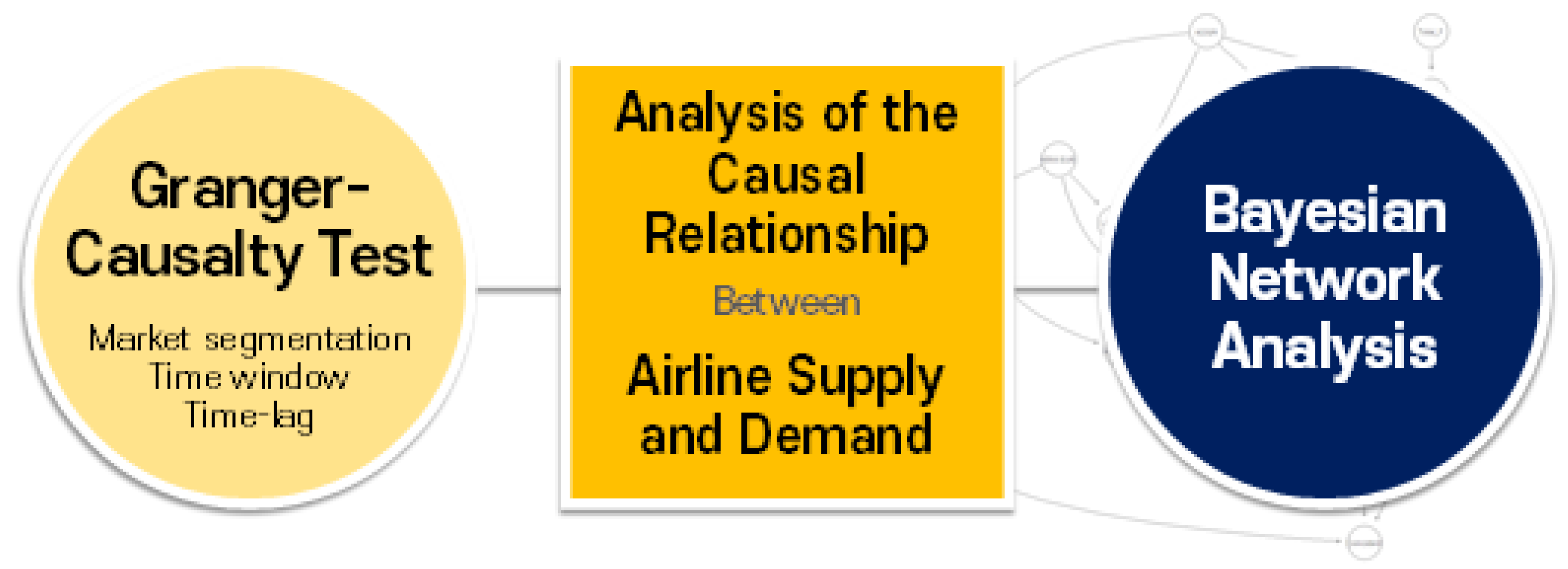
Figure 2.
Basic Analysis of Monthly Data Time Series Trends (by Market).
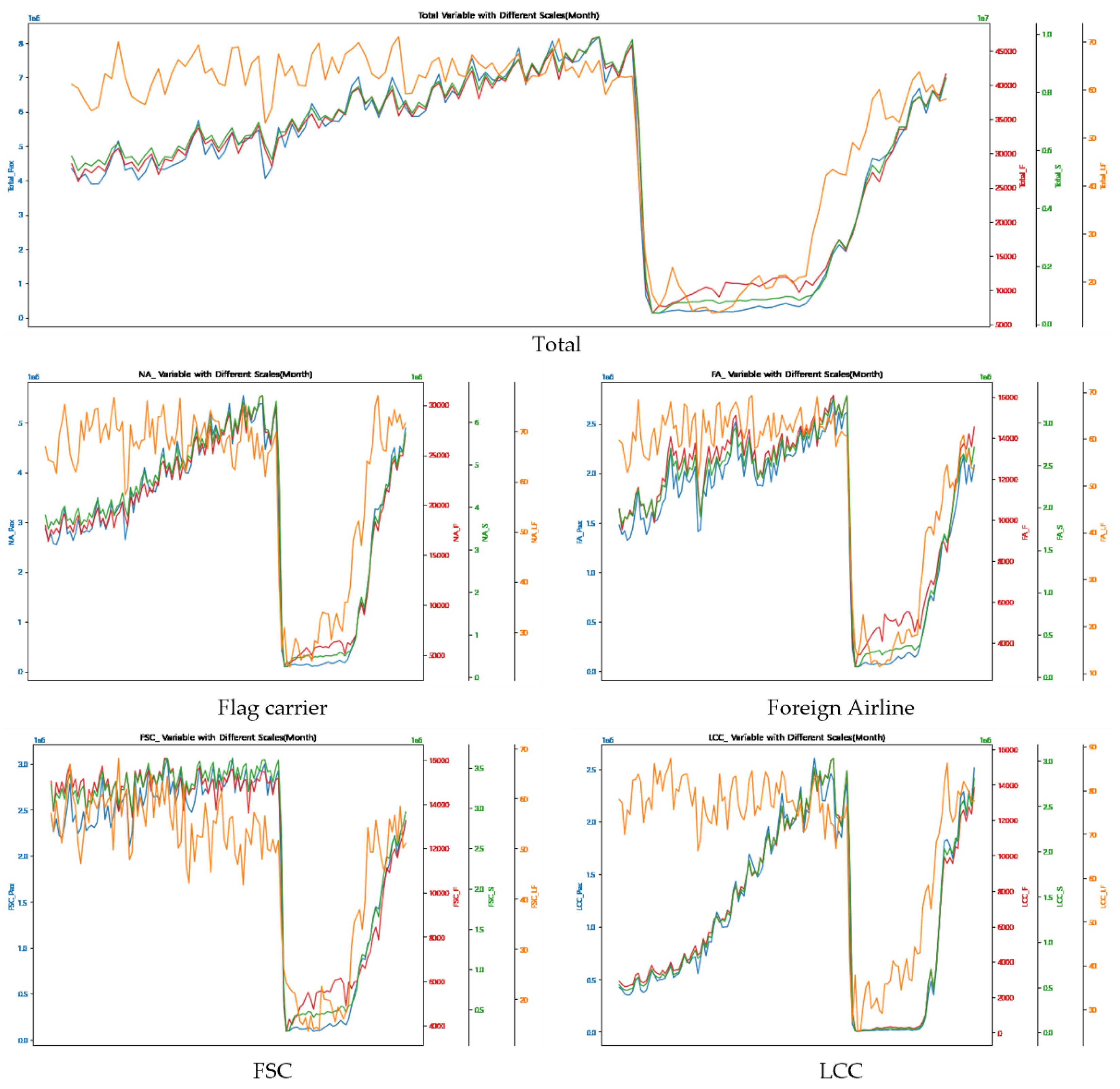
Figure 3.
Bayesian Network Results (Including Link Coefficients).
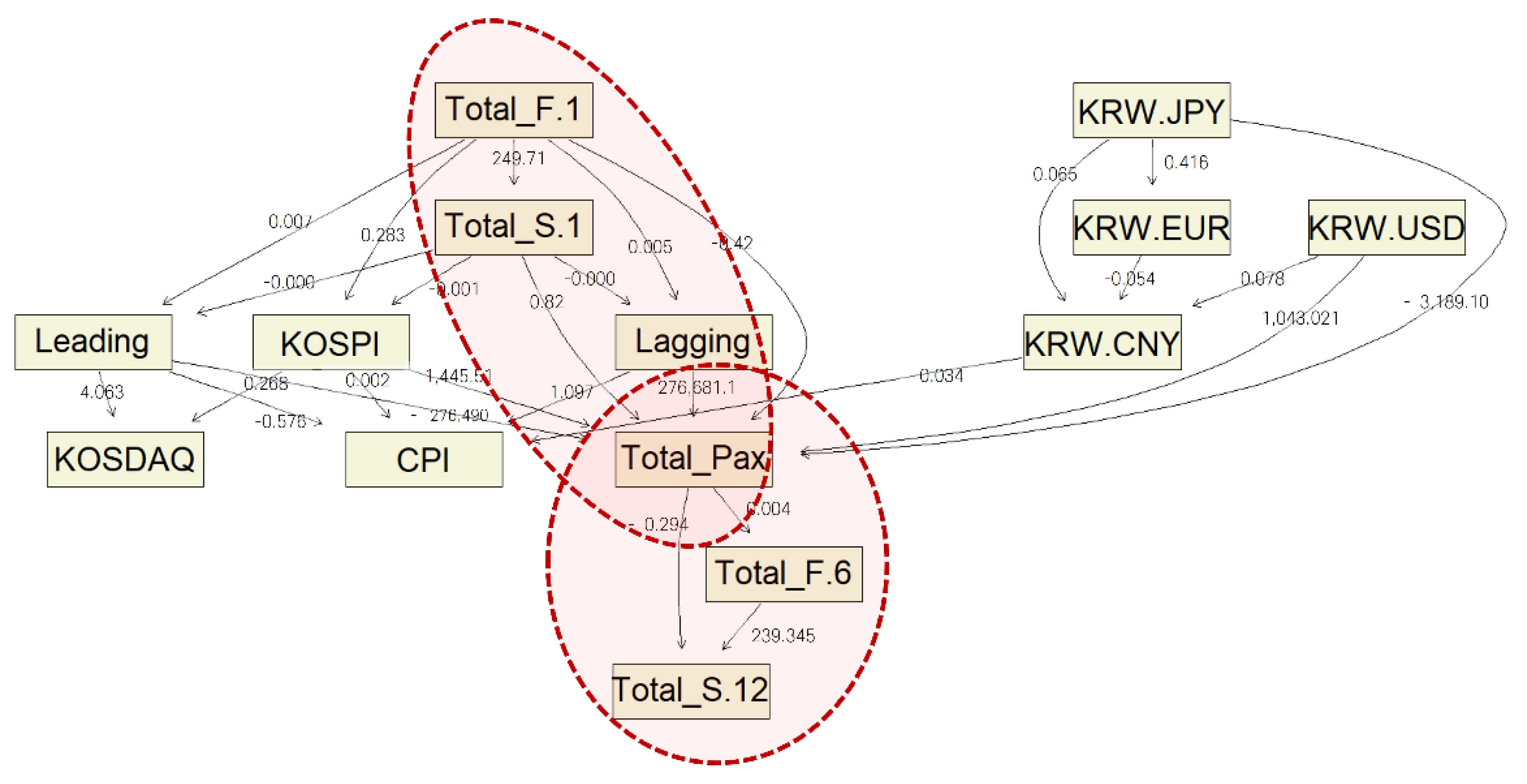
Table 1.
Time-Lag Settings by Data Segmentation.
| Category | Time-Lag Settings |
|---|---|
| Monthly (Month) | 1, 3, 6, 12, 18, 24, 36 |
| Quarterly (Quarter) | 1, 2, 3, 4, 6, 8, 12 |
| Yearly (Year) | 1, 2, 3, 5, 10 |
Table 2.
Classification of Variable Codes by Data Type.
| Type | Code | |
|---|---|---|
| Time Window | Month | M |
| Quarter | Q | |
| Year | Y | |
| Supply Variable | Frequency | F |
| Seats | S | |
| Load Factor | LF | |
| Demand Variable | Passenger | Pax |
| Market | Total | Total |
| Flag Carrier | Flag | |
| Foreign Airline | FA | |
| Full-Service Carrier | FSC | |
| Low-Cost Carrier | LCC | |
Disclaimer/Publisher’s Note: The statements, opinions and data contained in all publications are solely those of the individual author(s) and contributor(s) and not of MDPI and/or the editor(s). MDPI and/or the editor(s) disclaim responsibility for any injury to people or property resulting from any ideas, methods, instructions or products referred to in the content. |
© 2025 by the authors. Licensee MDPI, Basel, Switzerland. This article is an open access article distributed under the terms and conditions of the Creative Commons Attribution (CC BY) license (http://creativecommons.org/licenses/by/4.0/).
Copyright: This open access article is published under a Creative Commons CC BY 4.0 license, which permit the free download, distribution, and reuse, provided that the author and preprint are cited in any reuse.


