
Submitted:
24 March 2025
Posted:
26 March 2025
You are already at the latest version
Abstract
Objectives of measuring radon concentrations are radioprotection, as high concentrations in the atmosphere are hazardous agents, and scientific applications, mainly related to radon as an environmental tracer. For radon screening and surveying, usually relatively simple monitors are used such as track-etch or SSNTD detectors, while for scientific research, mostly more sophisticated and expensive equipment is employed. For some years, a new generation of instruments is available that were conceived as consumer grade monitors; however their performance is such that also their scientific usage appeared interesting for certain purposes. This requires particular QA/QC, including understanding their behaviour and knowing their limitations. One instrument in this hybrid consumer / science grade segment is the RadonEye, an ionization chamber with relatively high sensitivity. It has already been subjected to studies of its performance which suggest that it can be used also in certain scientific applications. This paper reports experiences with the RadonEye acquired during about two years, mainly for recording time series of radon concentration indoors and outdoors. Specific topics are calibration uncertainty, response to thoron and some so far unresolved questions related to measurement statistics.
Keywords:
RadonEye monitor
; calibration
; thoron
; counting statistics
1. Introduction
Because of its ubiquity and the possible risk that high concentrations of radon (Rn, in most cases dealing with 222Rn from the 238U decay chain) pose to human health (e.g. [1]), many studies have been, and continue to be performed world wide concerning its distribution and transport in the environment. A central element of radon studies is measuring its concentration in various environmental media and compartments.
Objectives of measuring radon concentrations are radioprotection and scientific applications, mainly related to radon as an environmental tracer. For radon screening and surveying, usually relatively simple monitors are used such as track-etch or SSNTD detectors, while for scientific research, mostly more sophisticated and expensive equipment is employed. For some years, a new generation of instruments is available that were conceived as consumer grade monitors; however their performance is such that also their scientific usage appeared interesting for certain purposes. This requires particular QA/QC, including understanding their behaviour and knowing their limitations. One instrument in this hybrid consumer / science grade segment is the RadonEye, an ionization chamber with relatively high sensitivity. It has already been subjected to studies of its performance, which suggest that it can be used also in certain scientific applications. Due to its fair price and easy usage, it also seems appropriate for Citizen Science (e.g., [2]) applications. However, good understanding of the behaviour of an instrument is essential for its QAed usage.
The objective of this paper is to discuss some features of the behaviour of the RadonEye, which have been observed during using it for about two years. Partly it is a sequel of the previous paper [3]. Its topics are calibration uncertainty, response to thoron and issues related to measurement statistics; specifically the occurrence of anomalies and the correlation of records from monitors operating in parallel under identical ambient conditions.
2. Materials and Methods
2.1. The RadonEye Monitor
This device manufactured by the South Korean company FTLab ([4]) has become increasingly popular for some years due to its fair price and relatively good performance, as documented through a number of QA studies reported in the literature. Basic properties are shown in company documents ([5,6]). For references on QA, see Sections 1.1 and 2.1 in [3]. It should be emphasized that QA tests in the references investigate the instruments under more or less standard conditions in terms of Rn concentration and environmental condition, mostly in controlled laboratory settings; this is different for the experiments reported here and previously in [3], with conditions partly far away from the ones specified by the manufacturers. This concerns very low (outdoor) Rn concentration and high humidity (although well protected from direct rain), low and high temperatures (although protected against direct sunlight) and possible vibrations induced by wind. This is to say that QA tests performed here are more severe and demanding than ones under laboratory conditions.
Calibration
The calibration procedure of the RadonEye is not really transparent. In the operation manual, a sensitivity 13.5 cpm/(1000 Bq/m³) is given. Apparently this is the default calibration factor. On the other hand, ([5]) says on p.1, “individually calibrated by equipments which are already calibrated to traceable international standards”, apparently meaning that the RadonEyes are individually calibrated through secondary standards. In this case, each device should have its particular calibration factor, but this number is not communicated. Again on the other side, [6] (Getting started, 1) says, “The device calibrates automatically and then starts measuring Radon”, which indicates some re-calibration when the RadonEye is started. Again [5] says, that “accuracy: <10% (min. error <0.5 pCi/l (±15Bq/m³))”, but it is not clear whether this relates to deviations from nominal concentration during the calibration procedure or to deviations during the operation of the device.
Initial experiments to verify the reproducibility (hence the validity of the calibration) are described in Section 2.2. The RadonEyes used for the experiments have serial numbers RE22207111958, HK01RE000496, HG04RE000641 and GJ17RE000076.
2.2. Parallel Exposure
Reproducibility of Rn concentration results was checked through parallel measurements with pairs of RadonEyes. The locations of measurements were Berlin (Par-1 and Par-2) and Vienna (Par-3), described in [3]. The setup of experiments Par-1 and Par-3 is shown in Figure 1. If calibration is correct, the statistics of the time series recorded under identical ambient conditions, in particular the mean over the measurement period, should be the same up to random statistical fluctuation.
2.3. Response to Thoron Exposure
Ionization chambers are sensitive against thoron (220Rn, Tn) along radon (222Rn). Since the internal construction of the device is not known to the user, we cannot say whether a diffusion barrier is installed to mitigate a possible Tn effect. To verify Tn sensitivity, in two experiments Tn-1 and Tn-2 a monazite concentrate layer (up to about 150 Bq/g 232Th) was placed on the bottom of a plastic container and the RadonEye on top, separated from the monazite by space holders (Figure 2). The devices were exposed for a few hours, and then removed and the decay recorded. Exposure was chosen higher in experiment Tn-2 than in Tn-1.
As experiment Tn-3, a RadonEye was placed into an improvised exhalation box (in fact a plastic ice cream container) oriented against a wall, Figure 2c). The objective was to see whether there is a significant difference compared to the exposure to the free room atmosphere about 1 m away (Figure 1a).
Theoretically, the activity of 212Pb (member of the 232Th decay series), called A2(t), follows (Figure 3a)
where λ1=0.0125 s-1 and λ2=1.810 e-5 s-1 the decay constants of Tn and 212Pb, A1=1 the Tn concentration inside the chamber (assumed constant). 212Bi and 208Tl are in approximate equilibrium with 212Pb after a few hours. (For a graph showing the full evaluation of the Bateman equation, see [7]. A convenient tool to evaluate decay chains is [8].) An analogous graph is shown in Figure 3b for the decay of 214Pb and 214Bi from the 238U series, with 214Pb set =1 at t=0.
A2(t) = (λ2/(λ2-λ1)) A1 (exp(-λ1 t)-exp(-λ2 t))
2.4. Anomalies
Anomalous Rn concentration values were observed. The fact was previously reported in [3]. The device concerned is RE22207111958, operated outdoors. Later the phenomenon disappeared; no physical explanation could be found. Closer examination showed no visible external humidity. The anomalies were also not related to vibrations due to wind gusts, particularly low temperature or similar possible causes.
Since only 1-hour means are stored, we cannot say whether the phenomenon occurred, or to which extent, also in the 10 minute-values, or if so, only during one isolated 10-min period or in several subsequent ones.
Two time series were investigated for anomalies. 1) The outdoor series #RE22207111958, mentioned above, and motivated by it, 2) the indoor series #GJ17RE000076, for which environmental effects can be excluded. With this monitor, the anomalous behaviour started in December 2024 after 10 months of continuous operation. The anomalies are less pronounced than the ones of the former monitor. The phenomenon ceased in early February 2025 and no similar anomalies were observed since (measurement is ongoing). The position remained the same and the ambient conditions of the monitor in the range of normal indoor temperature and humidity variation throughout the measurement.
Anomalous values in a time series are defined here (a) as isolated peaks and (b) as ones whose empirical occurrence frequency is much higher than the expected one. For series 1), this was visually obvious, while for 2) the presence of anomalies appeared visually likely in some instances, but further statistical reasoning was applied to confirm it. If in an interval, the expected number of instances with a certain count number is smaller than 1 but the observed number greater than 1, it can be supposed as anomaly. Specifically, the analysis is performed following [9]: In an interval of n hours in which the Rn concentration appears about stationary, defined as background, the mean count number m was calculated and defined as the expectation of a Poisson process. For each count value k in the interval, the Poisson prob(k’≥k) was computed, where
prob(k’≥k) = 1 – CumPoiss(k, m),
CumPoiss – the cumulative Poisson distribution, m – the mean within a window with about stationary background, excluding the instance for which the probability is evaluated, that is, the location of the suspected anomaly. The expected number of events is therefore n⋅prob(k’≥k), n – the number of instances in the window. Additionally, also following [9], the χ² value for observed vs. expected counts within a window, in which the background is about visually stationary, under the Poisson hypothesis is calculated. Reported Rn concentrations are converted into count numbers as shown in the following Section 2.5.
2.5. Correlation Between Parallel Time Series
Two RadonEyes were placed next to each other for the “parallel” experiments. The devices operated about synchronously with an offset of maximum 2 minutes which appears tolerable given the typical time constant of the natural Rn dynamic, not much less than an hour due to the physical inertia of atmospheric systems. (Starting them exactly synchronously is not easy.)
Because of measurement uncertainty which blurs the natural dynamic, the recorded series cannot be perfectly correlated (r=1). However, the lower the dynamic, the lower is the Pearson correlation.
As first step, we try to find out whether the observed correlation r between parallel and synchronously operating monitors can be explained by the inevitable uncertainty induced by the Poisson statistic of count numbers.
Analysis 1: Investigate whether the Poisson uncertainty is sufficient to explain a deviation of the correlation between two parallel measurements from unity.
Let X := x(i), i=1 … N, the counts representing an (unknown) true time series. The counts x are supposed Poisson distributed. Generate two series Y1 and Y2, with y1,2(i) ~ Poiss(x(i)) independently. These are regarded as the observed series. Compute r(Y1,Y2). Repeat many (J) times and compute 〈r〉, 〈.〉 the arithmetical mean over J realizations; check whether 〈r〉 is about equal the observed r. This would indicate that the deviation r<1 is indeed due to the Poisson counting statistic.
As X, an empirically observed series C(reported) is used substituting the unknown true one. From C(reported) we build an approximate expected series EC=C+1 (see Section 4.4 in [3]) The counts are estimated x=cint(EC cal), EC – expected Rn concentration, cal – calibration factor, cint – the rounding function. Next, the X are subjected to Poisson sampling, resulting in “Poissonized” series Z, which are converted into series Y that represent the observed Rn concentrations, by y=cint(z/cal). For generating Poisson deviates, the algorithm on p. 505 of [10] was used (also cited as Knuth algorithm on the Wikipedia page “Poisson distribution”).
The correlation between Y1 and Y2 derived from X by Poisson sampling depends on the magnitude of X. This is because the relative differences between xi and the derived y1 and y2 decrease with xi, because the Poisson standard deviation equals √xi, or relative 1/√xi. Therefore, the higher X in average, the more similar are Y1 and Y2 to X and hence to each other, so that the correlation between them increases →1. If one wants to test whether the correlation between two observed series X(1) and X(2), giving empirical r<1, can be explained by Poisson uncertainty, the simulated Poisson series Y(1)1 and Y(2)2 must be derived from X(1) and X(2) of equal average magnitude. This is achieved by rescaling one of the X(1) or X(2) to the other by multiplying with the ratio of their arithmetical means.
Analysis 2: If Poisson uncertainty is not sufficient to explain the deviation of the theoretical 〈r〉 from the empirically observed r (which is the case as will be shown), add noise according to a given model. The noise is quantified by a parameter σ, which is modified until 〈r(σ)〉 equals the empirically observed r. However, no physical error model underlies this reasoning. Formally, σopt := argmin |〈r(σ)〉-r| is defined as the σ that explains best the deviation of the observed r from 〈r(Poisson only)〉.
In absence of knowing the physical functioning of the detector in detail, the following noise models were considered:
“LN” – lognormal noise model: Gaussian distributed independent errors ε(σ)~N(0,σ), Z → W:=Z exp(ε) rounded to integers W1,2.
“ADD” – additive model: simply Z → W:= Z + ε, constrained to W>0. As modification, the model ε(σ)~U([-σ,σ]) was tried.
“MULT” – multiplicative model, Z → W:= Z⋅(1+ε), constrained to W>0.
“SQR±” – a super/sub-additive model, Z → W:= Z + (1±b/√(Z+1))ε. The denominator is chosen Z+1 to avoid eventual dividing by zero. For b, 0.2, 0.5, 1 and 2 were tried.
These models were chosen free-handed to cover a variety of “error behaviour”. Of course many more models can be conceived. The LN and MULT models are motivated by the idea that the error grows with Z, while it remains independent of Z for the ADD model. For the SQR± model, the error in-/decreases with lower Z.
2.6. Software
Standard statistics were performed with Excel and Past 4.17 [11]. Non-standard statistics such as the simulations in Section 2.5 were performed with home-made programs in QB64.
3. Results and Discussion
3.1. Deviation from Nominal Calibration
Three pairs of RadonEye monitors formed from four devices were operated in parallel next to each other, that is, under identical external conditions. The objective was to check whether individual calibration factors were equal up to statistical fluctuation. The three experiments are labelled Par-1 to Par-3 in the following. Table 1 shows which devices were combined into each pair. The respective parallel time series are shown in Figure 4.
It is shown that the mean Rn concentrations between the members of the pairs were not equal. The result is statistically significant, p<1e-3 (see table).
The relative biases were (58±12)%, (66±0.09)% and (44±0.05)% between monitor #1958 as reference, relative to monitors #0641, #0496 and #0076, respectively (see Table 1). This means that deviations between the latter three devices are at most 1.66/1.44=15%, which is higher than the declared accuracy bias <10% (Section 2.1).
None of the detectors has previously been exposed to high Rn concentrations. Therefore, different internal backgrounds are unlikely to be the reason for the discrepancy.
Hence, the only possible explanation is that actual calibration factors are significantly different. The Rn concentrations shown here result from the generic (default) calibration factor 1.35 cpm/(100 Bq/m³) = 0.81 cph/(Bq/m³) as given in the instruction sheet.
This means that the calibration factors of individual devices deviate from the nominal one rather substantially.
The Rn variability is essentially synchronous, as can be seen in the graphs of experiments Par-2 and Par-3 with Pearson r= 0.51 and 0.67, respectively. In experiment Par-1 the overall (natural) variability, which reflects weather episodes, was too small to allow an accurate assessment (r=0.22 only). The deviation of r from unity is further evaluated and discussed in Section 3.5.
3.2. Thoron Effect on the RadonEye
3.2.1. Experiments Tn-1 and Tn-2
The recorded nominal concentrations (not calibrated, because the RadonEye is not calibrated for Tn) are shown in Figure 5. The curves look differently from the theoretical curve (Figure 3), probably because the 1-hour recording period does not properly resolve the build-up phase controlled by the short half life of Tn (55.6 seconds).
LS fit of the decay tails for experiments Tn-1 and Tn-2 yield the estimated half lives 11.7 ± 1.6 h and 10.5 ± 0.2 h, respectively, well in agreement with the true 10.64 h half life of 212Pb.
3.2.2. Experiment Tn-3
Together with the 1-hour means that are stored by the RadonEye #1958, also 10-minute means were read from the display intermittently. The values are plotted in Figure 6. The subtracted background BG was estimated from the parallel operating device #0076, about half a meter away in the position shown in Figure 1b, considering the bias between the two devices (Section 3.1, Table 1: AM ratio).
The picture is less clear than in experiments Tn-1 and Tn-2. The very fast decrease after the end of exposure – poorly resolved by the 10 minute and 1 hour measurement intervals – indicates that the main contribution came from the progeny of 222Rn exhaled from the wall and perhaps some contribution of Tn. While an exhalation effect was clearly present, it was not strong enough for reliable quantification.
Perhaps a better made exhalation box and more careful BG control would allow better quantification. However, no substantial exhalation was expected in the building made of brick (probably made from local clay, as usual in Vienna at the time of construction, about 120 years ago). Additionally, the white lime coating acts as light barrier against Tn exhalation. In any case, the experiment showed the presence of contribution of exhalation from building material to indoor Rn concentration.
3.3. Anomalies
3.3.1. Series RE22207111958
A fraction of the time series that includes the anomalies is shown as Figure 7. Two clusters of anomalies can be recognized, but there appears no correlation between the anomalous peaks and they have no heads or tails, that is, they are isolated phenomena at least in the 1-hour resolution. After 28 October 2024 no further anomalies were observed. For further time series analysis (not shown here) the peaks were removed and replaced by the mean of the values left and right of the peaks. It should be noted that outdoor operation is not recommended by the manufacturer, but apart from these anomalies, the values appeared reasonable ([3]). So far, no similarly large anomalies were observed with RadonEyes operated indoors.
3.3.2. Series GJ17RE000076
As can be observed in Figure 8, suspected anomalies in this indoor time series are much less pronounced than the ones shown in the previous section. Some of these events, denoted by numbers in the figure, were investigated in more detail. The results are shown Table 2. The most relevant statistic is prob(k’≥k), meaning the probability that equally many or more counts would be registered at a given time under the Poisson hypothesis. Choosing p=0.01 as a (deliberate) threshold, we declare events with p<0.01 as anomalies. These registered counts are considered unlikely to result from a Poisson process within a window with approximately stationary background (assessed visually). The χ² statistic denotes whether the distribution within the window approximately conforms to Poisson, exploiting the fact that mean and variance are equal in this case. Figure 9 shows that the two statistics are essentially well aligned, as could be expected. Deviations may result from deviations from Poisson statistic or ill-definition of the background region, in that the assumption of stationary background was not sufficiently fulfilled.
Within a window, for the event (time) with the highest count number, the number of instances with equal or higher counts is equal 1 by definition. An observed event is likely an anomaly, if the expected number of events with higher or equal counts is far lower than 1. In Figure 10b (also introduced in [9]), event 17 (Table 2) shows the situation for a very significant anomaly; an opposite example is event 9, Figure 10a, which is well within what can be expected for a Poisson process, and therefore it is not an anomaly.
As a conclusion, also the monitor GJ17RE000076 shows some degree of anomalous behaviour, although much less pronounced than the GJ17RE000076. The physical reason is not known.
3.4. Missing Concentration Values
In [3], the fact was reported that certain concentration values were systematically missing. As a hypothesis, this may partly be caused by the rounding algorithm implemented in the RadonEye.
Since then, another RadonEye was acquired (#HK01RE000496) and the respective results are included here. The lowest missing values are summarized in Table 3. A satisfactory explanation for the finding is still missing.
3.5. Correlation Between Parallel Time Series
As “true” time series X the observed ones from experiments Par-1 to Par-3 were used.
3.5.1. Analysis 1
If Poisson uncertainty was sufficient to explain the deviation of the empirical r (Table 1) from unity, applying the “Poissonization” according to Section 2.4 of each series involved in the experiment should lead to 〈r〉 approximately equal to the empirical r. For example, in experiment Par-1, if series #0641 and #1958 were observations of the same (unknown) true series different only by Poisson uncertainty, their empirical r should be approximately equal to both 〈r〉 derived from #0641 and #1958, which should be approximately equal between them. Theoretical 〈r〉 are based on J=1000 realizations. The results are shown in Table 4. Figure 11 shows an example of an (in reality unknown) “true” concentration series and one realization of two “observed” series generated by Poisson sampling, representing the measured values of two RadonEyes. The targeted 〈r〉 is the mean over many (J) realizations of the correlation between the two “observations”. Additionally, in Table 4, the 〈r〉 for random series (X~U([1,a])), with a=5 and 10 for the series rnd-1 and rnd-2 are given. The finding that 〈r〉 of rnd-1 is lower than the one of rnd-2 illustrates what has been said in Section 2.4 about the necessity to rescale the input series before generating the Poisson simulated Y2 and Y2.
While the theoretical 〈r〉 are (1) approximately equal between the series of each pair (third column), they are (2) evidently very different from the empirically observed r. (1) can be interpreted that the shape (representing the dynamic) of each in a pair of series is about equal, only different by different means AM (Table 1). (2) means that there must be another error or noise component which decreases the correlation from 〈r(Poisson)〉 (the correlation expected if only Poisson statistic was responsible for r<1) to the empirical r.
3.5.2. Analysis 2
To investigate this further, independent errors are added to the series according to different models, suggested in Section 2.5.
For illustration of the effect of such added noise, Figure 12 shows an example of an (in reality unknown) “true” concentration series EC and three noisy series generated by adding a lognormal error, that is model LN, Cnoisy=EC exp(ε), ε~N(0,σ), representing the measured values of two RadonEyes, disturbed by noise. Since this noise is added independently to the two series that represent the parallel operating RadonEyes, 〈r〉 must decrease with σ increasing.
In the following, two models are presented: (1) the LN model; (2) the SQR+ model with b=0.5. The latter was chosen because it performed best among the models tried.
σ is modified until the resulting 〈r〉 equals the empirical correlation (Table 4 last column or Tab 1, second last row). Figure 13 shows the variation of 〈r〉 with σ increasing for two error models. Like in analysis 1, the mean results 〈r〉 are based on J=1000 realizations.
The σopt are given in Table 5. (1) The LN error model: While for each experiment, the σopt are similar for both series, they are not between the series. One might have expected that the devices behave similarly and therefore all σopt would be similar. Evidently this is not the case. (2) However, the discrepancy can be mitigated by varying the error model. SQR+ (b=0.5) yielded the lowest discrepancy, as can be seen by the σopt lying closer together in the right (b), than in the left (a) graph of Figure 13, but further optimization of the models may lead to a better result. For the latter model, the mean σopt equals 4.7 ± 0.6. This can be assumed a reasonable estimate for the non-Poisson error of the instrument, based on the SQR+ (b=0.5) error model. In any case, the physical meaning of the error models is unknown.
4. Conclusions and Recommendations
An inquiry was sent to the manufacturer of the RadonEye, FTLab, asking for assistance in solving some of the problems addressed here; specifically inconsistency of information about calibration (Section 2.1, 2.2 and 3.1) and missing values (Section 3.4). The request was rejected (e-mail 23.1.2025), citing trade secrets regarding the implemented algorithms. Regarding the anomalies (Section 3.3), the question for possible physical causes was answered in the sense that rare short instances of high Rn values may be caused by “floating particles including uranium or radium” and “interference by cosmic radiation and cases where the wavelength of a specific electromagnetic wave” generates such effect. The question for whether there exists a specific calibration factor for thoron was not answered.
The rather negative reaction is unfortunate because solving these problems would help improve the quality assurance of the RadonEye. The lack of this information certainly affects the usability of the device in scientific applications.
4.1. Calibration Issues
The parallel measurements showed that the default calibration factor is not really reliable. Accurate measurements require calibration of individual monitors for example through parallel measurements with science-grade instruments such as an Alphaguard or RAD-7 as secondary standards, or by direct calibration in a calibration chamber. Unfortunately, for normal citizens this is an expensive option (also noted in [12]). The preferable option would be that the manufacturer communicates the individual calibration of each device, which according to the instructions (Section 2.1) is apparently performed for each one. However, the manufacturer denied commenting the inconsistent information on calibration in the publicly available documents.
4.2. Thoron
The RadonEye is sensitive to thoron. Since long-lived decay products are deposited inside the chamber, the instrument has an increased background until these radionuclides have decayed. The relevant time scale is the half life of 212Pb, 10.64 hours, so that one must wait about 10 half lives or about 100 hours or 4 days until the background has practically disappeared. This behaviour has been expected. It shows, however, that one should avoid exposure to high concentrations to Rn, whose long-lived decay products are much longer lived than the ones of Tn, leading to persistent instrument background due to internal contamination. Indoors, Tn concentration is highest near walls, floors or ceilings, that is, close to building material that exhales the gas. Therefore, it is recommended to measure Rn some distance away from surfaces, because due to its short half life, the molecular diffusion length of Tn in the atmosphere is only 2.9 cm, although it can be transported further by advection or turbulent diffusion.
Experiment Tn-3 was aimed to detect Tn exhalation from the wall by positioning one device in an exhalation box close to the wall and one a distance away as background control. While the exhalation of Rn, together probably with Tn, could be confirmed, the result was not sufficiently reliable statistically. Future experiments with improved experimental set-up may yield more reliable evidence. In any case; the very simple feasibility of such experiments in principle was demonstrated.
4.3. Anomalies
The physical origin of the observed anomalies remained unknown. However, the finding shows that one should check the time series if high accuracy is required and in particular for devices operated in a mode not recommended by the manufacturer (outdoors, in this case). In both investigated cases the problem occurred after long continuous operation, but disappeared after some time. Although this cannot be proved, perhaps some kind of “vacation” should be granted to a monitor after long operation. It should be further discussed how to deal with the occurrence of anomalies. As long as anomalies are rare, they do not strongly affect the mean over some time, which is usually the main objective of measurement, but time series must be interpreted with care.
4.4. Statistical Issues, Missing Concentration Values
The problem of missing values (Section 3.4) could not be solved because the manufacturer does not disclose necessary information about internal data processing.
Results of RadonEyes running parallel and synchronously under the same external conditions are less correlated than one would expect if the uncertainties were only due to Poisson statistics of count numbers. Hence there must be other sources of uncertainty which blur the correlation. In absence of knowledge about the physical functioning of the device, several error models were tried. A reasonable model of the non-Poisson error seems to be a super-additive error Z+δZ (Z – the count number) of the kind δZ = (1+0.5/√(Z+1))ε, ε~N(0,σ), σ≈4.7, found by trying.
Future detailed investigations possibly involving some kind of back-engineering may shed more light on these issues.
4.5. Citizen Science and Professional Use
The experiments show that the RadonEye monitor can also be used in Citizen Science; not only for surveying and monitoring which is the usage for which the RadonEye has been conceived, but also in an educative context: Simple experiments about response to sudden shifts of the Rn source term, basic considerations related to measurement statistics and to time series analysis can be performed easily.
For professional use, certain precaution must be taken. If the objective is accurate values of Rn concentration, re-calibration and assessment of the internal background seem inevitable. This is most easily done by secondary calibration under varying Rn concentrations. (First experiments have been performed in this direction, to be communicated in a future publication.) If the objective is the investigation of temporal dynamics and correlation with Rn predictors and proxies, the exact value of Rn concentration is not so important.
If the objective is legal-proof assessment whether a room or a building conforms to a regulatory standard, either re-calibration is necessary or accounting for considerable calibration error in the uncertainty budget. Methodology into this direction can be found in [13].
Ongoing research is concerned with correlation of Rn with causal or proxy-type predictors such as meteorological variables including atmospheric stability, ambient dose rate and concentrations of air pollutants.
Funding
This research received no external funding.
Data Availability Statement
The Rn time series are available on justified request.
Conflicts of Interest
The author declares no conflict of interest.
References
- Hajo Zeeb, Ferid Shannoun (eds): WHO handbook on indoor radon: a public health perspective, 2009. https://www.who.int/publications/i/item/9789241547673 (accessed 14.1.2025).
- Vohland, K.; Landzandstra, A.; Ceccaroni, L.; Lemmens, R.; Perelló, J.; Ponti, M.; Samson, R.; Wagenknecht, K. (Eds.) The Science of Citizen Science; Springer International Publishing: Berlin/Heidelberg, Germany, 2021. [CrossRef]
- Bossew P., Benà E., Chambers S., Janik M. Analysis of outdoor and indoor radon concentration time series recorded with RadonEye monitors. Atmosphere 2024, 15, 1468. [CrossRef]
- Radon FTLab (no year): http://radonftlab.com/ (accessed 14.1.2025).
- Radon Eye operation manual, Model RD 200, no year. https://merona.blob.core.windows.net/radonftlab-web/20220404_RadonEye_%EC%82%AC%EC%9A%A9%EC%9E%90%EC%84%A4%EB%AA%85%EC%84%9C(%EC%98%81%EB%AC%B8).pdf (accessed 14.1.2025).
- No title, no year: https://www.radonshop.com/mediafiles/Anleitungen/Radon/FTLab_RadonEye-RD200/FTLab_RadonEye_ManualEN.pdf (accessed 20.3.2025).
- Radon-220 (Thoron) decay chain (https://www.mathworks.com/matlabcentral/fileexchange/69157-radon-220-thoron-decay-chain ), MATLAB Central File Exchange. (Accessed 11.1.2025).
- EPA, Radionuclide Decay Chain (n.y.): https://epa-prgs.ornl.gov/cgi-bin/radionuclides/chain.pl (accessed 21.1.2025).
- Bossew P., Kuča P., Helebrant J. True and spurious anomalies in ambient dose rate monitoring. Radiation Protection Dosimetry 2023, 199(18), 2183–2188; [CrossRef]
- Devroye, Luc (1986). “Discrete Univariate Distributions”. https://luc.devroye.org/chapter_ten.pdf (accessed 20.1.2025).
- Hammer, Ø., Harper, D.A.T., Ryan, P.D. 2001. PAST: Paleontological statistics software package for education and data analysis. Palaeontologia Electronica 2024, 4(1): 9pp. http://palaeo-electronica.org/2001_1/past/issue1_01.htm. Download: https://www.nhm.uio.no/english/research/resources/past/ (accessed 20.3.2025).
- Beck T., Foerster E., Biel M., Feige S. Measurement Performance of Electronic Radon Monitors. Atmosphere 2024, 15, 1180. [CrossRef]
- Tsapalov, A.; Kovler, K.; Bossew, P. Strategy and Metrological Support for Indoor Radon Measurements Using Popular Low-Cost Active Monitors with High and Low Sensitivity. Sensors 2024, 24,4764. [CrossRef]
Figure 1.
Parallel exposure, experiments Par-2 (a) and Par-3 (b). On the picture (b) a Radiacode dose rate monitor can be seen.
Figure 1.
Parallel exposure, experiments Par-2 (a) and Par-3 (b). On the picture (b) a Radiacode dose rate monitor can be seen.
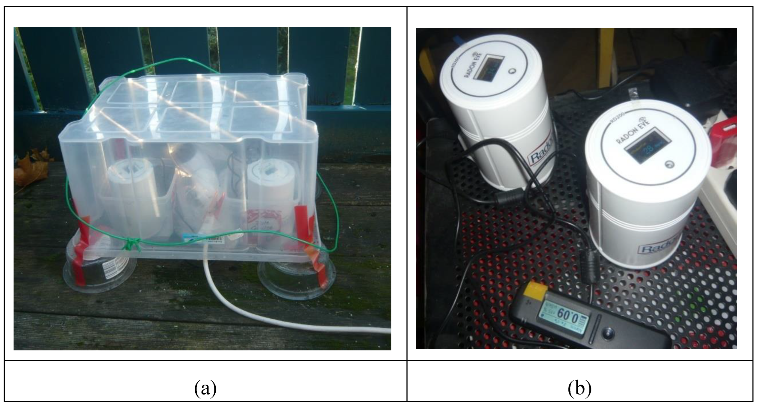
Figure 2.
Thoron exposure experiments: Tn-1 (a), Tn-2 (b) and Tn-3 c).
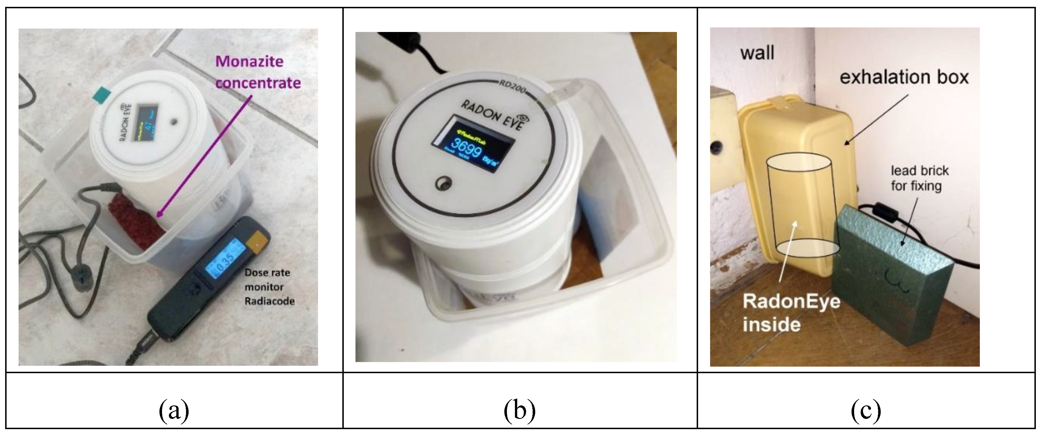
Figure 3.
(a) Theoretical activity of 212Pb in the chamber, relative to the Tn concentration A1 set as 1. (b) Theoretical activities of 214Pb and 214Bi in the chamber, relative to the 214Pb concentration set as 1 at t=0.
Figure 3.
(a) Theoretical activity of 212Pb in the chamber, relative to the Tn concentration A1 set as 1. (b) Theoretical activities of 214Pb and 214Bi in the chamber, relative to the 214Pb concentration set as 1 at t=0.
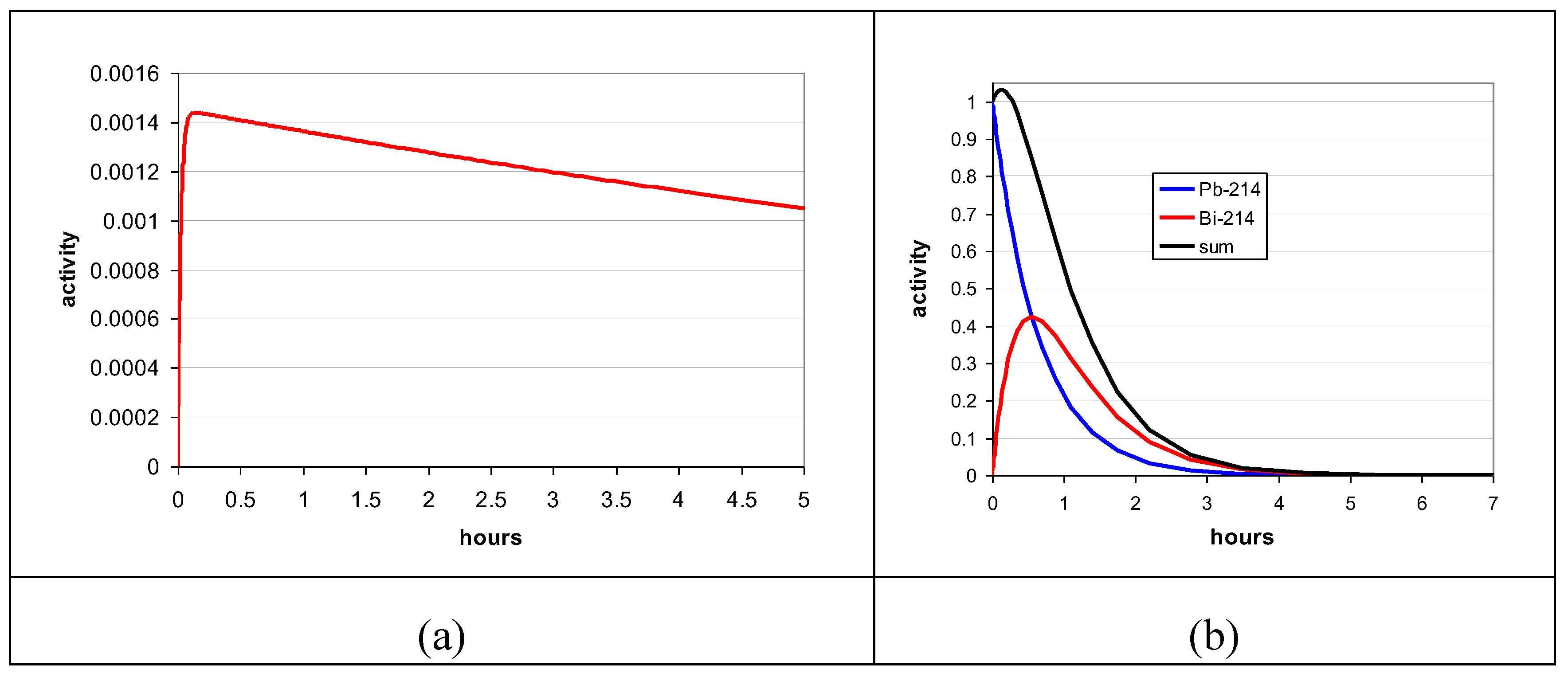
Figure 4.
Analyzed parallel time series; from top to bottom: experiments par-1, par-2, par-3; y-axis: Rn concentrations (1 hour mean) in Bq/m³, retrieved through the Smartphone app.
Figure 4.
Analyzed parallel time series; from top to bottom: experiments par-1, par-2, par-3; y-axis: Rn concentrations (1 hour mean) in Bq/m³, retrieved through the Smartphone app.
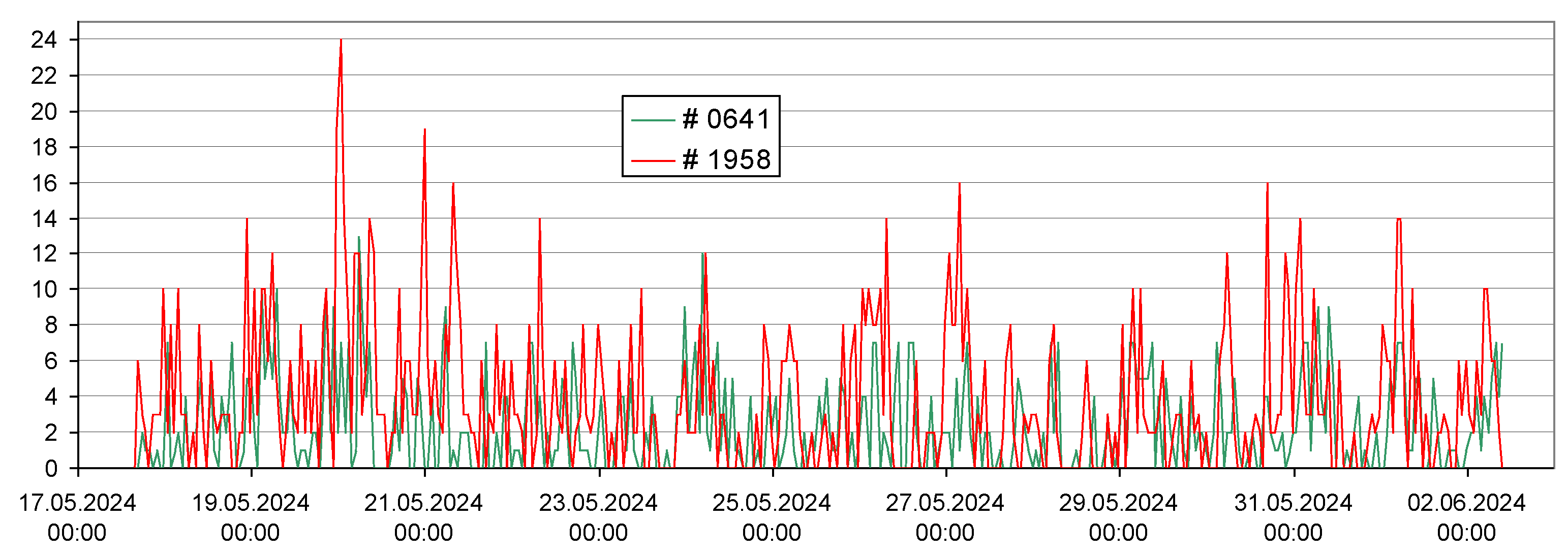
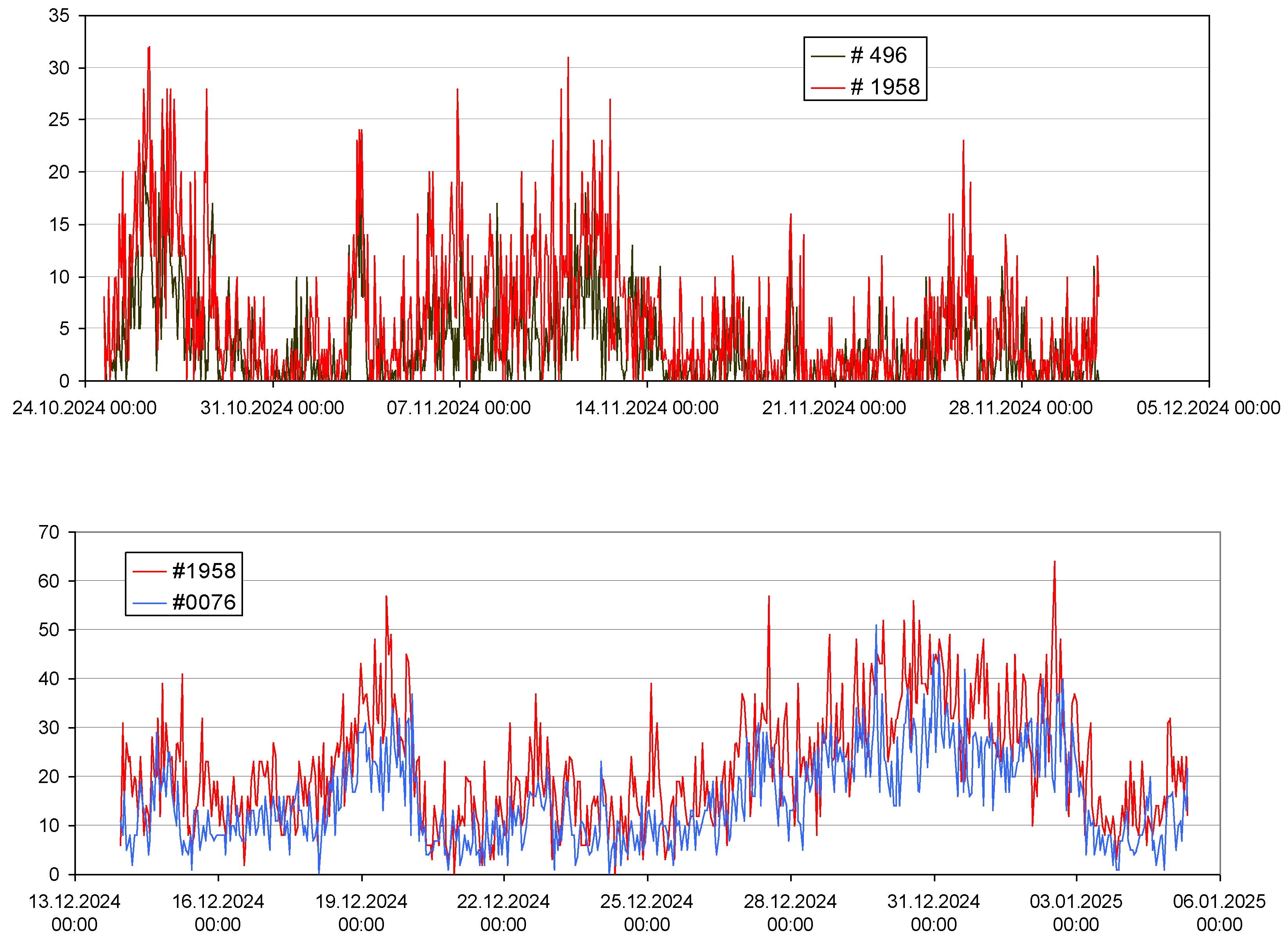
Figure 5.
(a) experiment Tn-1, time series; BG = 4.95 Bq/m³, estimated from data before Tn exposure; (b) experiment Tn-2, BG=22.3 Bq/m³.
Figure 5.
(a) experiment Tn-1, time series; BG = 4.95 Bq/m³, estimated from data before Tn exposure; (b) experiment Tn-2, BG=22.3 Bq/m³.
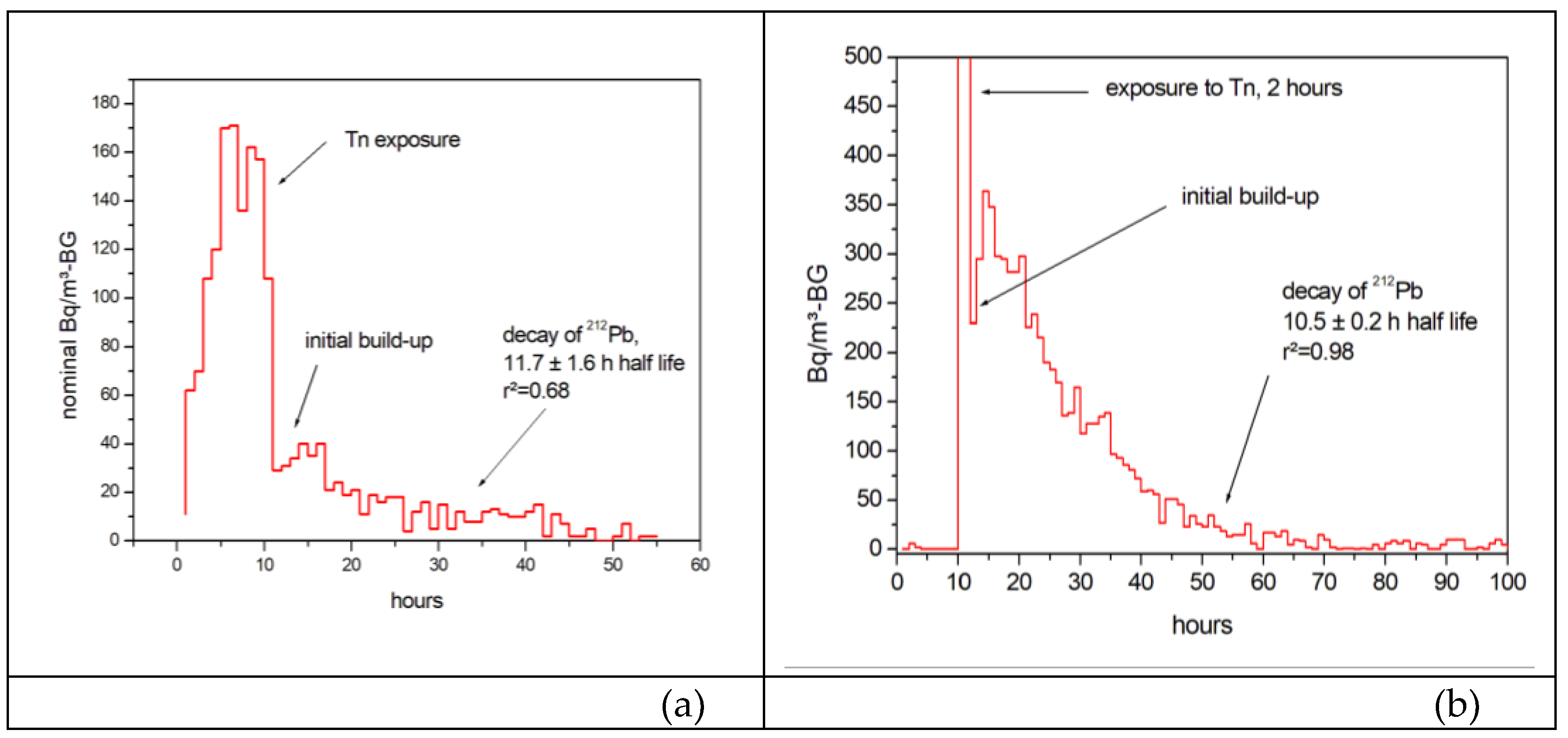
Figure 6.
Experiment Tn-3: (a) Time series of the RadonEye values; green: 1-hour means, blue dots: 10 minute means; f: double exponential with half lives 26 minutes and 10.5 hours. (b) 10-minute values only and fitted double-exponential function.
Figure 6.
Experiment Tn-3: (a) Time series of the RadonEye values; green: 1-hour means, blue dots: 10 minute means; f: double exponential with half lives 26 minutes and 10.5 hours. (b) 10-minute values only and fitted double-exponential function.
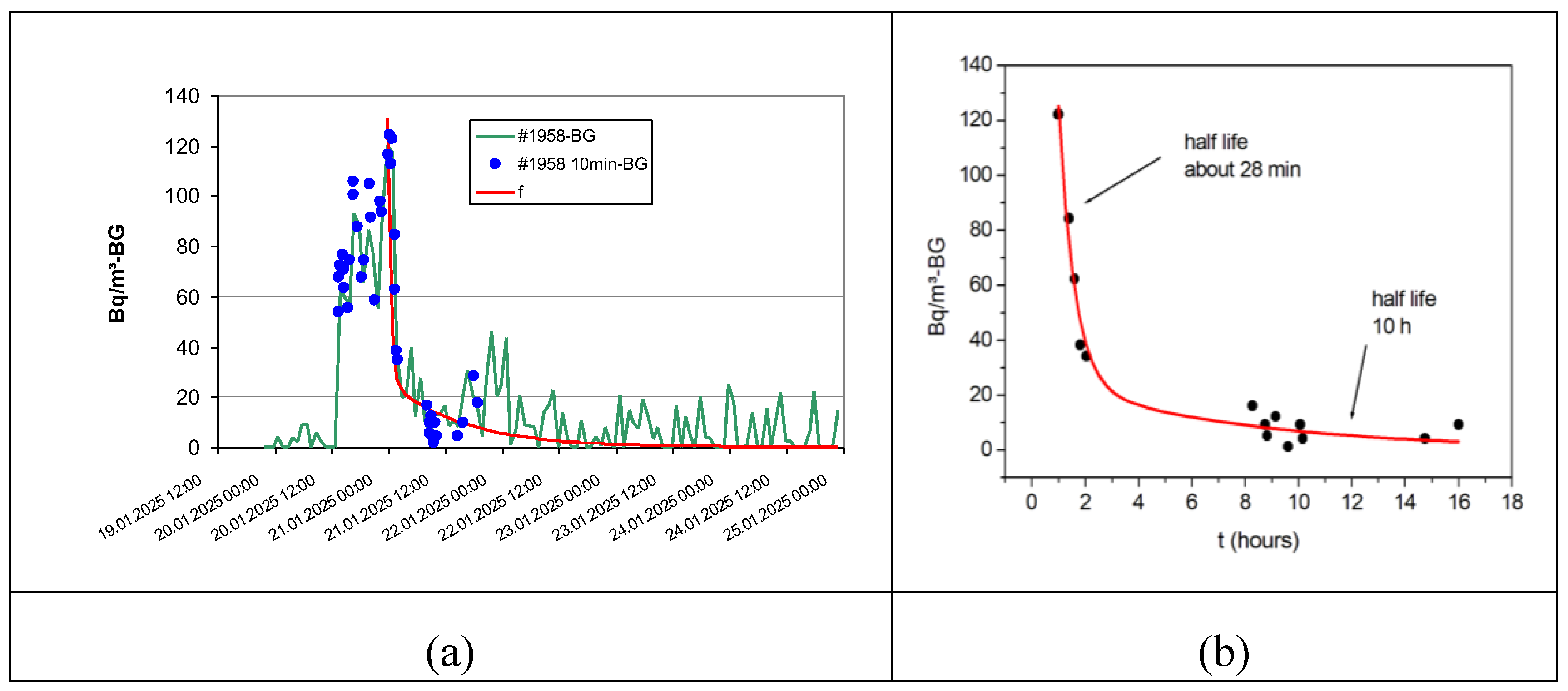
Figure 7.
A series of anomalies in a Rn time series. (a) the complete set of anomalies, October 2024; (b) magnification of the cluster 19.-23.10.2024.
Figure 7.
A series of anomalies in a Rn time series. (a) the complete set of anomalies, October 2024; (b) magnification of the cluster 19.-23.10.2024.
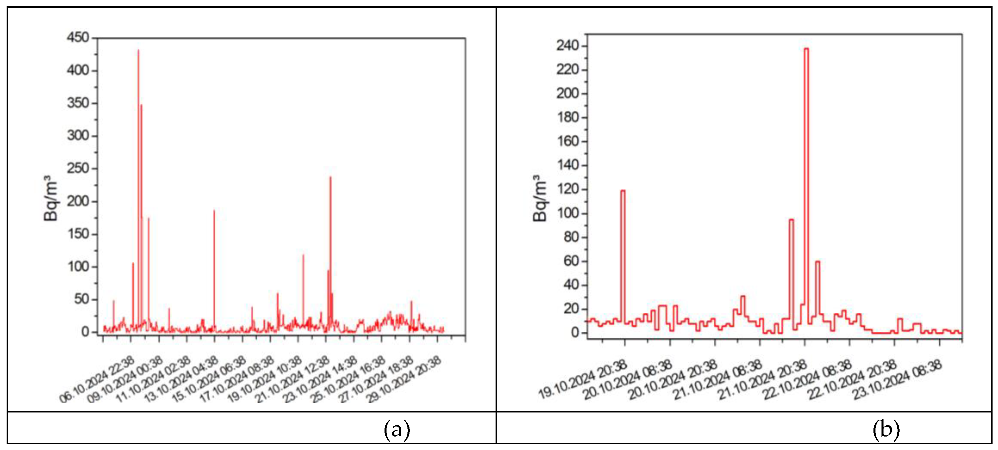
Figure 8.
Time series including suspected anomalies, late 2024 – early 2025. The numbers denote events investigated in more detail, Table 2.
Figure 8.
Time series including suspected anomalies, late 2024 – early 2025. The numbers denote events investigated in more detail, Table 2.
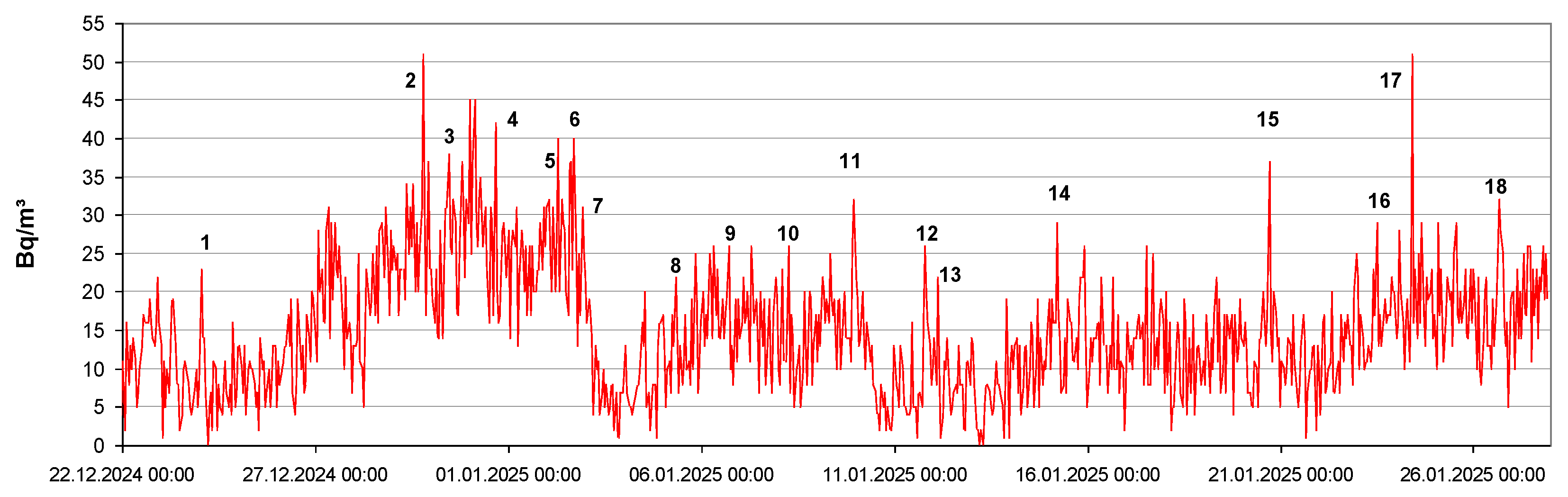
Figure 9.
Scatter plot of two statistics (see text). The numbers refer to the event labels in Table 2.
Figure 9.
Scatter plot of two statistics (see text). The numbers refer to the event labels in Table 2.
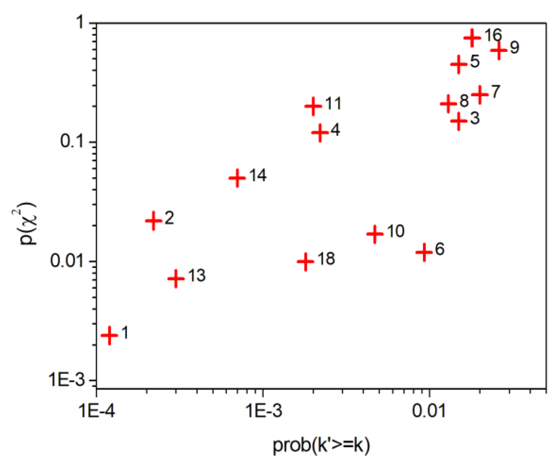
Figure 10.
Expected vs. observed numbers of counts ≥ the numbers given in the data labels. (a) event 9, (b) event 17 (see Table 2). If the expected occurrence of the highest count number is far lower than 1, as for event 17 (b), the presence of an anomaly can be assumed. Blue line: theoretical location for the Poisson hypothesis.
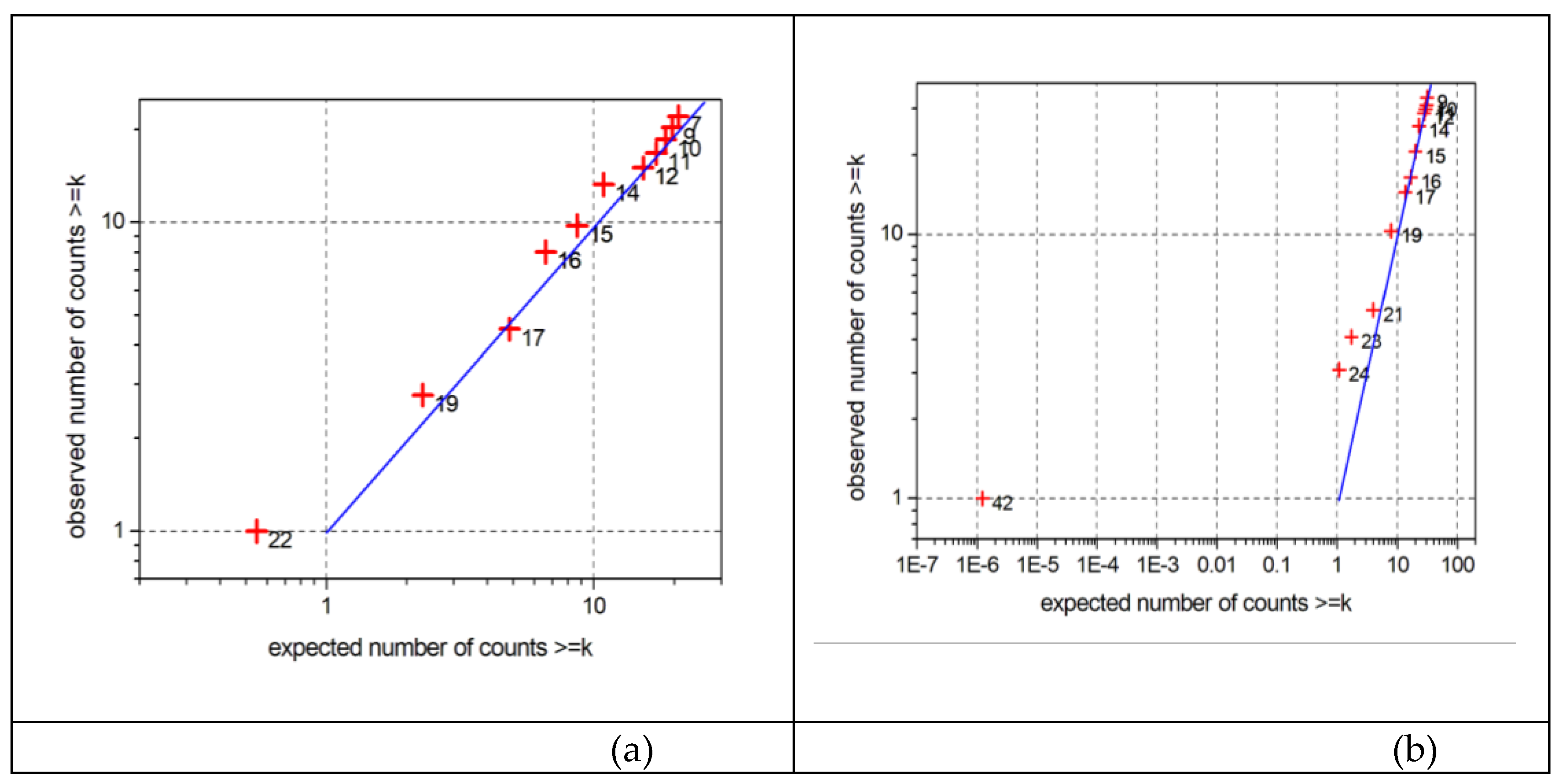
Figure 11.
Example of a “true” Rn series (black) and two simulated “observed” series (orange and blue). (See text for details.).
Figure 11.
Example of a “true” Rn series (black) and two simulated “observed” series (orange and blue). (See text for details.).
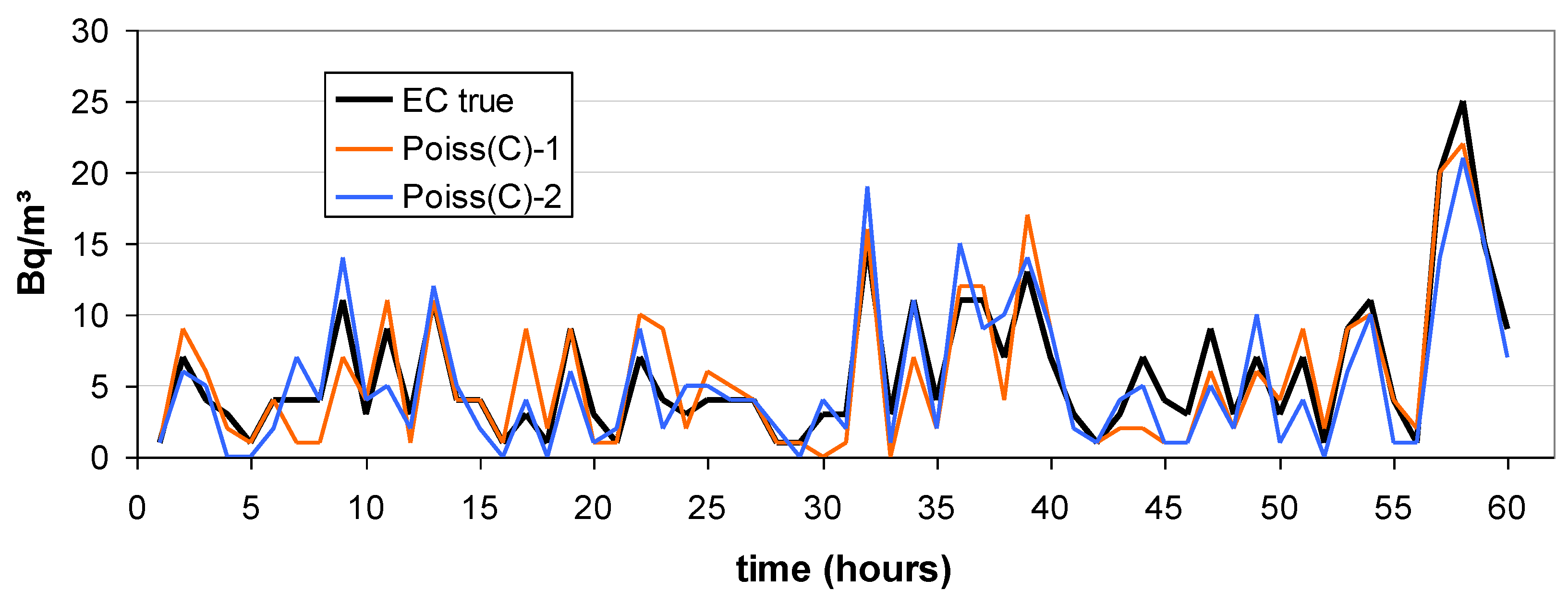
Figure 12.
Example of a “true” Rn series (black) and three “noisy” series, different by the σ of the lognormal Gaussian error (error model LN) added. Legend: value of σ in N(0,σ).
Figure 12.
Example of a “true” Rn series (black) and three “noisy” series, different by the σ of the lognormal Gaussian error (error model LN) added. Legend: value of σ in N(0,σ).
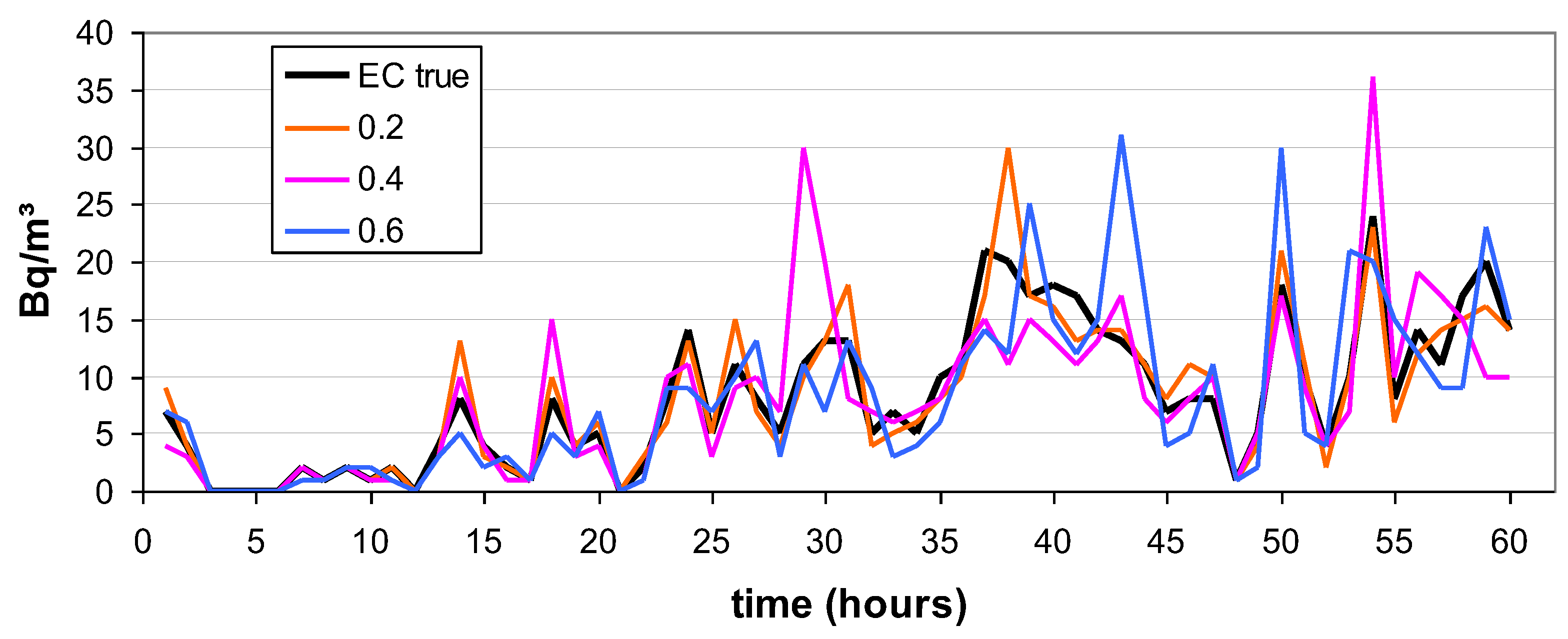
Figure 13.
Theoretical correlation between parallel operating monitors, in dependence on added, quantified by σ. (a) LN model; (b) SQR+ model. The arrows point to the values of σopt, for which the theoretical 〈r(σ)〉 equals the empirical one.
Figure 13.
Theoretical correlation between parallel operating monitors, in dependence on added, quantified by σ. (a) LN model; (b) SQR+ model. The arrows point to the values of σopt, for which the theoretical 〈r(σ)〉 equals the empirical one.
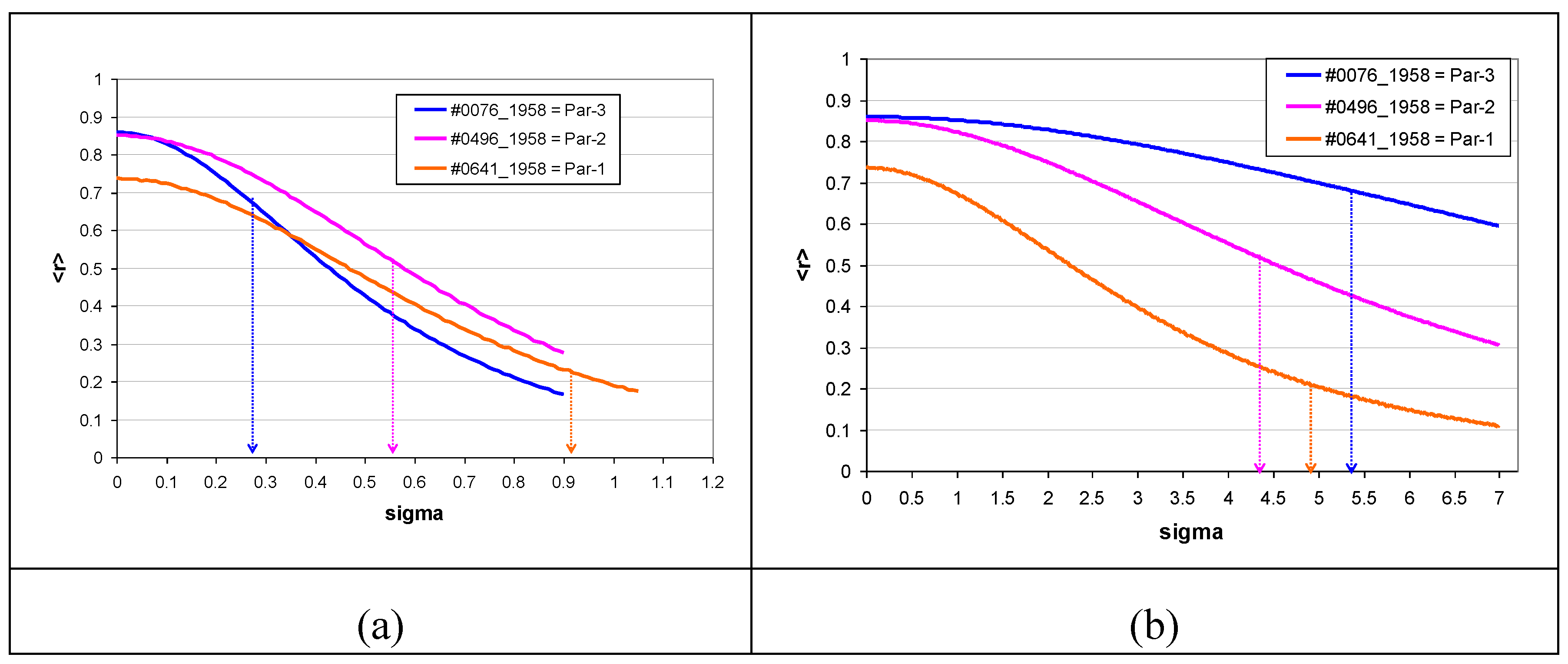

Table 1.
Results of the experiments par-1 to par-3. n – number of data (=hours); AM, SD, SE – arithmetic mean, standard deviation and error; p-values for t – t-test; M-W – Mann Whitney; F – F-test; K-S and A-D – Kolmogorov Smirnov and Andersen Darling tests for equal distribution. Printed red: ratio between the first and second AM ± SE. Device# are the last 4 digits of the serial numbers, see Section 2.1.
| Experiment | par-1 | par-2 | par-3 | |||
| Device# | #1958 | #0641 | #1958 | #0496 | #1958 | #0076 |
| Date | 17.5.-2.6.2024 | 24.10.-3.11.2024 | 13.12.2024-5.1.2025 | |||
| n | 379 | 893 | 538 | |||
| AM | 3.8 | 2.4 | 5.8 | 3.5 | 22.1 | 15.4 |
| SD | 4.0 | 2.6 | 6.2 | 4.1 | 11.8 | 9.1 |
| SE | 0.20 | 0.13 | 0.21 | 0.14 | 0.51 | 0.39 |
| AM1/AM2 ± SE | 1.58 ± 0.12 | 1.66 ± 0.09 | 1.44 ± 0.05 | |||
| paired test | ||||||
| t | 9.2e-11 | 6.7e-36 | 2.3e-54 | |||
| sign | 2.0e-7 | 1.7e-21 | 8.0e-43 | |||
| Wilcoxon | 6.0e-10 | 2.1e-34 | 8.5e-49 | |||
| unpaired | ||||||
| t(uneq var) | 3.7e-9 | 7.1e-21 | 3.5e-24 | |||
| M-W | 9.6e-7 | 2.2e-16 | 1.2e-21 | |||
| F eq var | 6.9e-18 | 1.9e-33 | 5.2e-9 | |||
| K-S | 1.2e-8 | 4.0e-22 | 1.7e-16 | |||
| A-D | 0 | 0 | 0 | |||
| correlation | ||||||
| Pearson r | 0.22 | 0.51 | 0.67 | |||
| Spearman ρ | 0.20 | 0.48 | 0.68 | |||
Table 2.
Characteristics of the suspected anomalies shown in Figure 8. Rn – reported radon concentration; cts k – estimated number of counts; BG – background. Printed red: probably not anomalous.
Table 2.
Characteristics of the suspected anomalies shown in Figure 8. Rn – reported radon concentration; cts k – estimated number of counts; BG – background. Printed red: probably not anomalous.
| event # | date | Rn | cts k | BG (cts) | prob(k’≥k) | p(χ²) |
|---|---|---|---|---|---|---|
| 1 | 24.12., 0:48 | 23 | 19 | 6.94 | 1.2e-4 | 0.0024 |
| 2 | 29.12., 18:48 | 51 | 42 | 22.93 | 2.2e-4 | 0.022 |
| 3 | 30.12., 10:48 | 38 | 32 | 21.00 | 0.015 | 0.15 |
| 4 | 31.12., 15:48 | 42 | 35 | 20.50 | 0.0022 | 0.12 |
| 5 | 2.1., 6:48 | 40 | 33 | 21.82 | 0.015 | 0.45 |
| 6 | 2.1., 16:48 | 40 | 33 | 21.00 | 0.0093 | 0.012 |
| 7 | 2.1., 21:48 | 31 | 26 | 16.6 | 0.020 | 0.25 |
| 8 | 5.1., 7:48 | 22 | 19 | 10.67 | 0.013 | 0.21 |
| 9 | 6.1., 16:47 | 26 | 22 | 13.85 | 0.026 | 0.59 |
| 10 | 8.1., 5:47 | 26 | 22 | 11.74 | 0.0047 | 0.017 |
| 11 | 9.1., 22:47 | 32 | 27 | 14.41 | 0.0020 | 0.20 |
| 12 | 11.1., 18:47 | 26 | 22 | 8.09 | 3.9e-5 | 6.0e-6 |
| 13 | 12.1., 2:47 | 22 | 19 | 7.50 | 3.0e-4 | 0.0072 |
| 14 | 15.1., 4:47 | 29 | 24 | 11.33 | 7.0e-4 | 0.050 |
| 15 | 20.1., 16:47 | 37 | 31 | 10.22 | 1.3e-7 | 1.8e-5 |
| 16 | 23.1., 11:47 | 29 | 24 | 14.87 | 0.018 | 0.75 |
| 17 | 24.1., 9:47 | 51 | 42 | 15.87 | 3.8e-8 | 1.2e-4 |
| 18 | 26.1., 15:48 | 32 | 27 | 14.32 | 0.0018 | 0.010 |
Table 3.
Systematically missing nominal concentration values of four RadonEye devices.
| device id. | missing concentration values (Bq/m³) |
|---|---|
| GJ17RE000076 | 3, 6, 9, 12, 15, 18, 21, 24,... |
| RE22207111958 | 1, 4, 5, 7, 9, 11, 13, 15, 17, 18,... |
| HG04RE000641 | 3, 6, 8, 11, 13,... |
| HK01RE000496 | 3, 6, 9, 12, 15, … |
Table 4.
Theoretical correlations 〈r〉 ± standard deviation between parallel time series. The series represent the X(1) and X(2) (Section 2.4), the 〈r〉 the correlations between Y(1)1 and Y(1)2, and Y(2)1 and Y(2)2, respectively. Empirical r from Table 1.
Table 4.
Theoretical correlations 〈r〉 ± standard deviation between parallel time series. The series represent the X(1) and X(2) (Section 2.4), the 〈r〉 the correlations between Y(1)1 and Y(1)2, and Y(2)1 and Y(2)2, respectively. Empirical r from Table 1.
| Experiment | series | 〈r〉 ± SD | empir. r |
|---|---|---|---|
| Par-1 | #0641 | 0.738 ± 0.0235 | 0.22 |
| #1958 | 0.735 ± 0.025 | ||
| Par-2 | #0496 | 0.851 ± 0.010 | 0.51 |
| #1958 | 0.821 ± 0.011 | ||
| Par-3 | #0076 | 0.860 ± 0.009 | 0.68 |
| #1958 | 0.829 ± 0.015 | ||
| rnd-1 | 0.514 ± 0.030 | ||
| rnd-2 | 0.703 ± 0.020 |
Table 5.
Optimal noise parameters σopt for two noise models.
| Experiment | series | σopt | empir. r | |
|---|---|---|---|---|
| model LN | model SQR+, b=0.5 | |||
| Par-1 | #0641 | 0.92 | 4.76 | 0.22 |
| #1958 | 0.92 | 4.89 | ||
| Par-2 | #0496 | 0.56 | 4.42 | 0.51 |
| #1958 | 0.52 | 3.80 | ||
| Par-3 | #0076 | 0.26 | 5.54 | 0.67 |
| #1958 | 0.22 | 4.58 | ||
Disclaimer/Publisher’s Note: The statements, opinions and data contained in all publications are solely those of the individual author(s) and contributor(s) and not of MDPI and/or the editor(s). MDPI and/or the editor(s) disclaim responsibility for any injury to people or property resulting from any ideas, methods, instructions or products referred to in the content. |
© 2025 by the authors. Licensee MDPI, Basel, Switzerland. This article is an open access article distributed under the terms and conditions of the Creative Commons Attribution (CC BY) license (http://creativecommons.org/licenses/by/4.0/).
Copyright: This open access article is published under a Creative Commons CC BY 4.0 license, which permit the free download, distribution, and reuse, provided that the author and preprint are cited in any reuse.


