Submitted:
28 August 2024
Posted:
28 August 2024
You are already at the latest version
Abstract
This research reviews a novel artificial intelligence (AI) based application called ‘TLDetect’, which filters and classifies anomalous glow curves (GCs) of thermoluminescent dosimeters (TLDs). Until recently, GCs review and correction in the lab were performed using an old in-house software, which uses Microsoft Access database and allows the laboratory technician to manually review and correct almost all GCs without any filtering. The newly developed application ‘TLDetect’ uses a modern SQL database and filters out only the necessary GCs for technician review. TLDetect first uses an Artificial Neural Network (ANN) model to filter out all regular GCs. Afterwards, it automatically classifies the rest of the GCs into five different anomaly classes. These five classes are defined by GCs typical patterns, i.e. high noise at either low or high temperature channels, untypical GC width (either wide or narrow), shifted GCs whether to the low or to the high temperatures, spikes, and the last class contains all other unclassified anomalies. By this automatic filtering and classification, the algorithm substantially reduces the amount of technician’s time of reviewing the GCs and makes the external dosimetry laboratory dose assessment process more repeatable, accurate and fast. Moreover, a database of GCs class anomalies distribution over time is saved along with all their relevant statistics, which can later assist with preliminary diagnosis of TLD reader hardware issues.
Keywords:
TLD
; Machine learning: Glow curves
; anomaly classification
; correction
; dosimetry
1. Introduction
Radiation workers worldwide are being monitored for occupational ionizing radiation exposure by national dosimetry services. The ionizing radiation exposure routine monitoring cannot be underestimated, since the safety of workers is on stake. For this reason, all over the world, across medical, industrial and nuclear sectors, all workplaces try to maintain high quality and precision exposure measurements of eye lens and whole body doses [1,2,3,4,5,6,7,8,9,10,11,12,13]. Thermoluminescence dosimetry is a widespread technology for performing personal occupational dosimetry, which measures x-ray, gamma, beta, and thermal neutron radiation. The dose is estimated using a reader that heats the thermoluminescent dosimeter (TLD) element and reads the current initiated by the emitted photons. This current is proportional to the radiation exposure. The measured output current of the thermoluminescence (TL) as a function of the heating rate is called a glow curve (GC), and its integral is proportional to the radiation absorbed by the dosimeter. Figure 1 shows a representative example for a GC.
The research was conducted using a Thermo Harshaw 8800 reader, and TLD cards of type LiF:Mg,Ti. The reader uses the default time-temperature profile (TTP) of 25ºC per second in order to heat the TLD elements. Cards of type LiF:Mg,Ti possess a complex GC containing at least 10 different glow peaks (GPs) ranging from room temperature to 400°C. The main GP, referred to as peak number five, used for dosimetry in these card type at this TTP appears at about 205°C. Since the estimation of dose as accurately as possible is of great importance for dosimetry labs, a lot of efforts are invested on the analysis of GCs and on the quality assurance of the entire dosimetry process.
It is important to meticulously assess the quality of glow curves prior to the dose estimation in a method that is as automated as possible [14]. Over the past two decades, numerous Computerized Glow Curve Analysis (CGCA) techniques have been developed and studied [15,16,17,18], as well as deconvolution methods to reveal various TLD glow peaks [19,20]. Some have been employed to determine parameters of kinetic models [21], while others have focused on improving the accuracy of instrumental background assessment for low-dose assessments or implementing internal quality criteria to detect anomalies [22,23]. Additional applications of CGCA have aimed at identifying specific anomalies within glow curves [24].
One of the earliest applications of ML for TL dosimetry [25] used an artificial neural network (ANN) to estimate doses in LiF:Mg:Ti-based four-element dosimeters. More recently, researchers have demonstrated the applicability of ML algorithms in TL dating [26], classification of thermoluminescence features of natural halite (rock-salt) [27], estimating the response by fading time [28], estimating the irradiation date out of TL GCs [29], obtaining the TL dosimetric properties of calcite obtained from nature [30] and lastly there have been even efforts to utilize machine learning methods to detect different kinds of anomalies in Thermoluminescent Dosimeter (TLD) glow curves [31,32,33,34,35]. Other researches tried to predict the GC distortion pattern due to the variations in the TTP [36] and utilize them to determine corrected TL counts from anomalous GCs as if their shape was normal.
However, none of these methods have culminated in a comprehensive application that integrates both artificial intelligence (AI) techniques and a complementary classical deterministic algorithm to fully filter and classify glow curve anomalies and propose some means of automatic corrections when possible.
Good quality GCs have a unique characteristic shape (see Figure 1 and Figure 3), while anomalous or extremely low dose GCs are mostly distinguished by their abnormal shape [37,38]. The specific shape anomalies of GCs depend on various factors such as organic contamination of the polytetrafluoroethylene (PTFE) cover on the TLD element, which may arise from dirty fingers, aging of PTFE foils causing them to separate and to transfer heat less efficiently to the TLD element, nitrogen flow problems during hot-gas heating of the TLDs, different pre- and post-irradiation annealing procedures, the exact position of the TLD element between PTFE foils that was set during the TLD card mounting, static electricity, electrical network interruptions, and more[39,40,41].
The relation between a GC anomaly shape and its hardware related possible cause may help us identify in advance suspicious trends that can indicate hardware problems [35,42]. The specific shape and characteristics of GCs depend on various parameters. By carefully analyzing anomalies in GCs, it is possible to detect and identify troubling trends that may signal real HW issues. Identifying these trends in advance, might prevent a decline in EDL performance and consequently improve the accuracy of occupational doses estimation.
Specifically, the identification of the next four different sub-classes can give the laboratory signs regarding future hardware problems:
- -
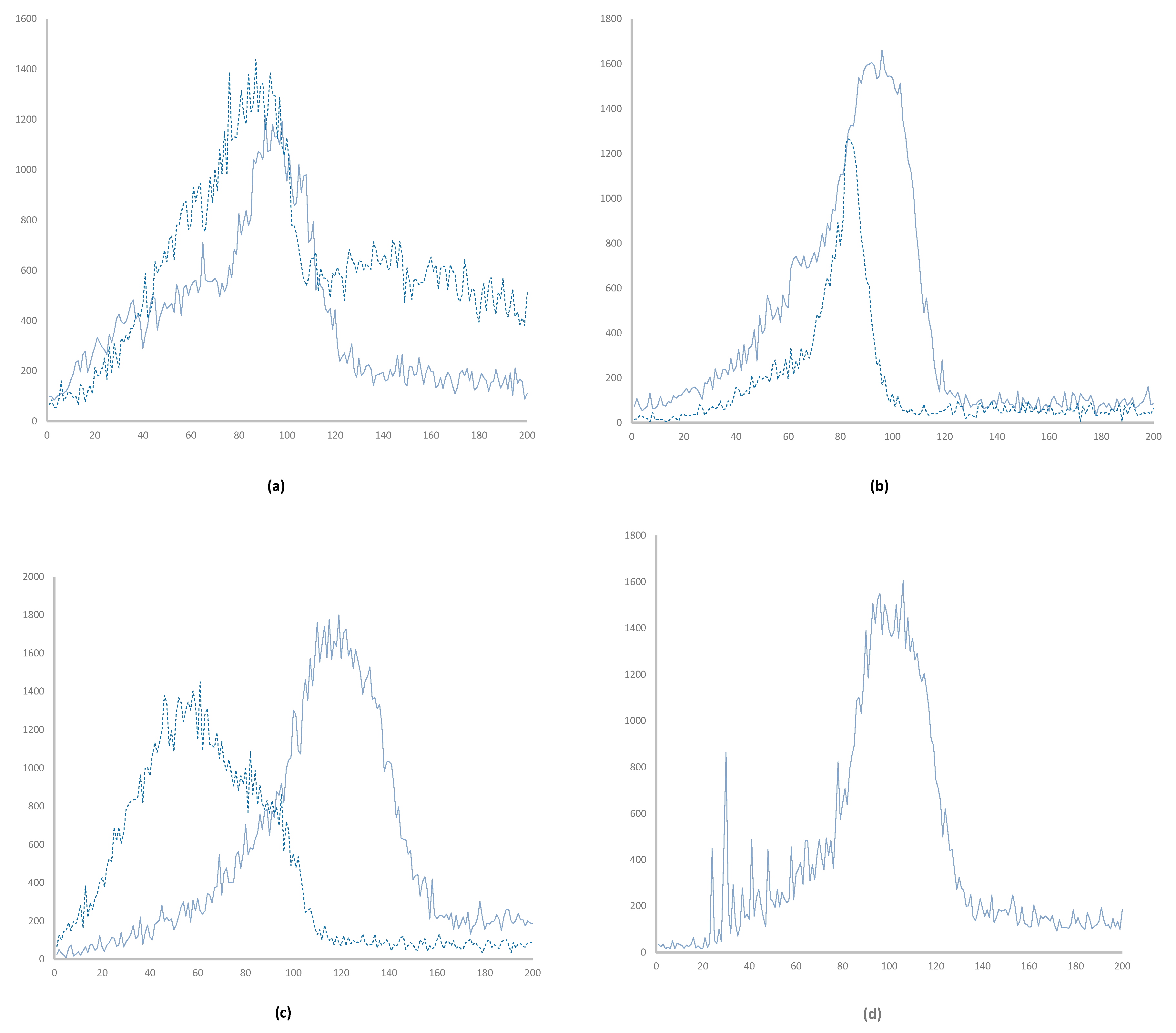
- Class A Low (Figure 2a) is characterized by high TL signal at low temperatures. Possible reasons causing this anomaly include: organic (usually carbon) contamination of the Teflon cover on the TLD element, from user’s dirty fingers, aging of Teflon foils, which causes them to split from TLD element and to transfer heat less efficiently to the TLD element, nitrogen flow problems during heating of the TLD elements by hot-gas, and residual radiation from a prior exposure to a relatively high dose.
- -
- Class A High (Figure 2a) is characterized by high TL signal at high temperatures. Some possible reasons causing this anomaly include: pre- and post-irradiation annealing procedures, TLD heating rate issues (GPs move to higher temperatures as the heating rate increases), and spectral response of either the photocathode or other optics such as IR filters.
- -
- Class B Wide (Figure 2b) is characterized by wide GPs compared to normal GPs. Some possible reasons for this anomaly include: TLD batch characteristics, the position of the TLD element between Teflon foils that was set in the factory, aging of Teflon foils, which causes them to split from TLD element and to transfer heat less efficiently to the TLD element.
- -
- Class D Spikes (Figure 2d) is characterized by spikes over the GC. These spikes may be caused by static electricity (especially in TLD readers, which are located in extremely low humidity areas), light emanates from burning particles, which arise from contamination on the TLD sample surface or on the Teflon foils from either dust or oily fingerprints, electrical network interruptions, or reader electronic interferences.
On top of automatically classifying the anomalous GCs, the ‘TLDetect’ application also suggests an automatic correction in some cases. Dosimeters with GCs that cannot be corrected by ‘TLDetect’ are presented to the laboratory technician for specific examination and manual correction if needed. As the categorization of GC anomalies is a subjective task (there is no single clear definition for describing these anomalies) we had to carefully define some typical anomaly classes and develop the appropriate mathematical conditions and constraints that characterize these anomalies. The classes that we defined for the possible anomalies are detailed in Table 1. Examples of all anomaly classes, which are listed in Table 1 are shown in Figure 2.
Figure 2.
Example illustrations of the different glow curve anomaly classes: (a) is class A (Low and High) (b) is class B Narrow and class B Wide (c) is class C (Low and High) and (d) is class D having spikes. The y axes of all sub-figures is in arbitrary units, and the x axes are channel number.
Figure 2.
Example illustrations of the different glow curve anomaly classes: (a) is class A (Low and High) (b) is class B Narrow and class B Wide (c) is class C (Low and High) and (d) is class D having spikes. The y axes of all sub-figures is in arbitrary units, and the x axes are channel number.
TLDetect SW & Pipeline
The current process of examining and correcting the GCs is a tedious process that consumes precious laboratory technician’s time each month. After the examination, the data of the GCs are entered into Thermo © WinAlgo algorithm [43], which outputs the skin dose Hp(0.07) and penetrating dose Hp(10) of each dosimeter, which are the ionizing radiation dose equivalents penetrated into a depth of 0.07 mm and into a depth of 10 mm under the skin accordingly.
The new developed ‘TLDetect’ application is planned to replace the current one. ‘TLDetect’ connects to the database of the Thermo © readers (TLD Harshaw 8800), filters out all good quality GCs using an AI filter, and automatically classifies the GCs into the anomaly classes while also enabling an automatic correction for class A anomaly, significantly reducing the long manual process currently carried out in the lab each month. ‘TLDetect’ is also expected to improve the repeatability and accuracy of examination of the GCs, reduce human errors, shorten the training processes in the laboratory, and save about 50 monthly work hours.
2. Materials and Methods
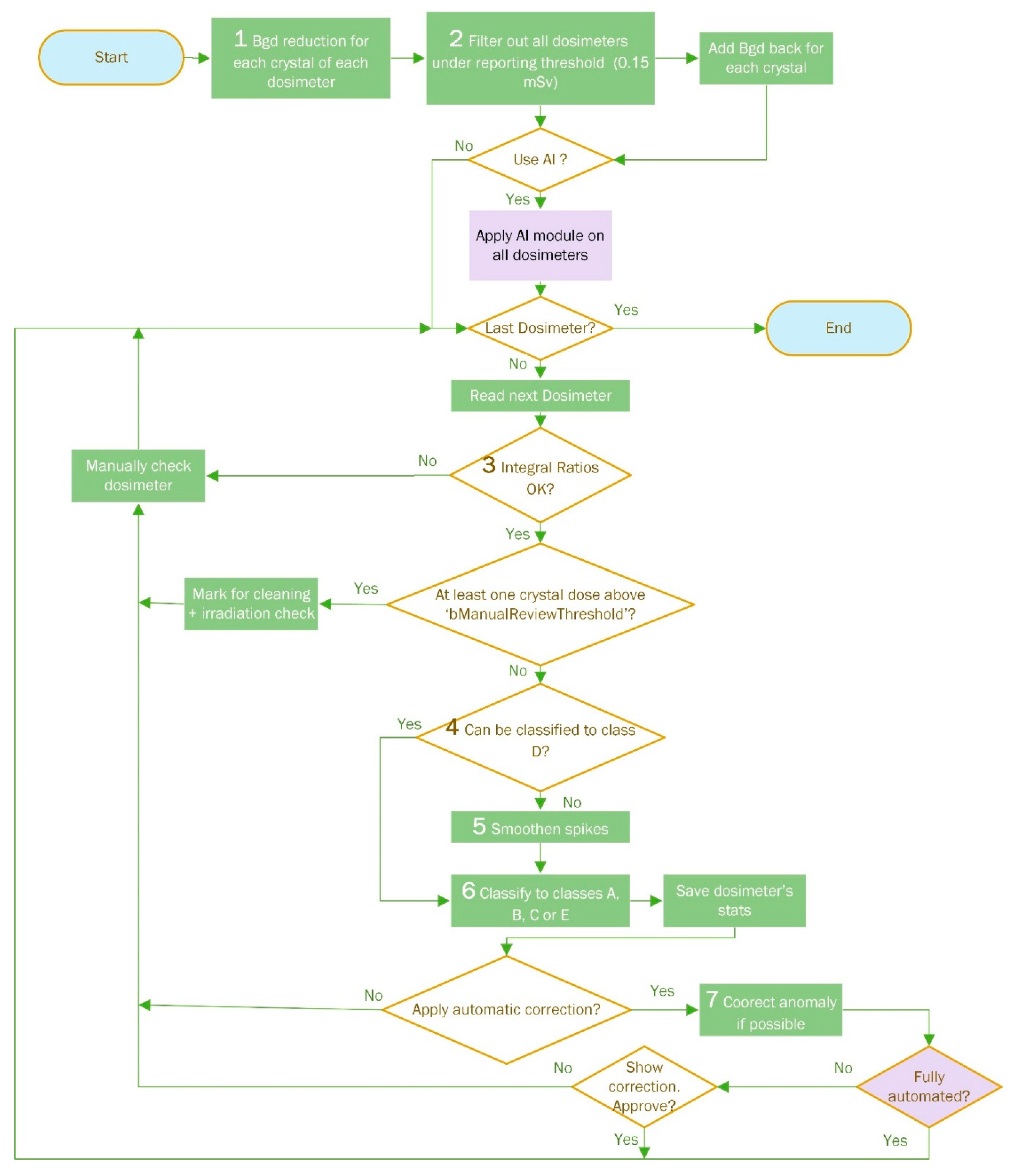
The algorithm high level description is shown in Figure 3. In Table 2 we show a list of all algorithm parameters, their meaning, and their data type. The TLDetect application has been characterized and developed using all necessary parameters for adjusting each of the sub-algorithms that classify the GCs into each class, for defining the formulas in it and for controlling the transition between the different stages of the algorithm.
Figure 3.
The algorithm’s high level flow chart. The purple parts are optional stages for the user’s choice. The bold numbers at the beginning of some chart stages are references for detailed explanations of these stages in coming section.
Figure 3.
The algorithm’s high level flow chart. The purple parts are optional stages for the user’s choice. The bold numbers at the beginning of some chart stages are references for detailed explanations of these stages in coming section.
Detailed Algorithm Stages Review
Inside ‘TLDetect’ algorithm block diagram which is shown in high level view in Figure 3, all the referenced stages are explained in detail in the following sub-sections. Additionally, at the associated equations when denoting, we refer to the value of the GC at channel i.
- i.
- Background reduction
This stage is referenced inside Figure 3 by the digit 1. The reduction amount is calculated by:
where ‘Bgd’ is the calculated background radiation to be subtracted, ‘radiationPerWeek’ is a configuration file parameter that is set to 1 [mrem/week], (day2 - day1) is the number of days passed between former measurement of the dosimeter and the current one. If the value turns out to be negative, we set the value to 1 mrem. This way ‘Bgd’ accumulates the expected background ionizing radiation over the desired period of time, where the weekly accumulation is 1 mrem. ‘Bgd’ value is saved per dosimeter in order to add it back when needed in the next filtering stage.
- ii.
- Filtering out low dose dosimeters
This stage is referenced inside Figure 3 by the digit 2. After background reduction, TLDetect filters out all dosimeters that are under the reporting level, meaning those dosimeters whose crystals (either 3 or 4 elements) accumulated dose of at most 16 mrems after background reduction, i.e. their total dose would be less than the 20 mrems reporting level.
- iii.
- AI Filter for normal GCs
After filtering out low dose dosimeters, ‘TLDetect’ uses a pre-trained deep learning ANN in order to filter out all dosimeters that have a regular shape. All the remaining dosimeters, which are suspected as anomalous GCs, are directed to next filters. Example regular GCs that were filtered by the ‘TLDetect’ algorithm are shown in Figure 4.
The ANN was trained using a total of 1608 different GCs, 144 of them were anomalous GCs and the rest were different examples of normal GCs. The network itself contained 3 inner layers of depths 5, 15 and 5 nodes each. The input layer contained 202 nodes – one node for each of the 200 channels, and 2 more inputs – one for the Kurtosis and the second for the Skewness of the GCs – both of them are good features that contributed to the ability of the algorithm to classify anomalous GCs as they represent measures of the distribution shape. The output of the ANN was a single number encompassing the probability of the GC being a normal one. The more the probability is closer to 1 the more the GC’s shape is similar to that of a normal GC. We used 60% of the labeled GCs for the training process, 20% for the validation and the last 20% for testing. It is interesting to note that we took a low decision threshold for normal GC classification of value of 0.91. We chose this number since we were tolerant for the filter to give us false negative classification (the algorithm classifies normal GCs as anomalous ones) but we did not want it to give us false positive classifications (the algorithm classifies anomalous GCs as normal ones).
- iv.
- Integral ratios filter
This stage is referenced inside Figure 3 by the digit 3. Using two conditions, it checks that all 3 or 4 crystal doses lie inside element ratios that reflect possible radiation fields [5], and only in this case ‘TLDetect’ continues to the next stages of the classification. The first condition is applied using Eq. 2. If it is true then algorithm passes to the next stage, if it is false then the second condition is checked using Eq. 3 where each crystal triplet or quadrat should match at least one line in Table 3. If the second condition is met then the algorithm passes to the next stage, if it is false then ‘TLDetect’ classifies this dosimeter for manual inspection.
where
where both Crystals_Quotient and ratio_table_threshold are parameters defined inside the configuration file.
- v.
- Class D classification smoothening
This stage is referenced inside Figure 3 by the digit 4. ‘TLDetect’ first tries to classify the GCs into class D, which is spikes class (Figure 2.d).
If the GC is classified to class D, then the algorithm will not try to classify it to another class and will continue to the next GC. On the other hand, if the algorithm cannot classify the GC to class D, it will smoothen it before continuing to next filters. Experience shows that spikes mostly have either one channel or two channels width. In order to check for spikes, the algorithm checks Eq. 4 with its three conditions – the first condition must be satisfied and either one of the second or third one – for all channels i from 1 to 197:
where is the value of GC at channel i and ‘SpikesNeighDiff’ is a configuration file parameter. If TLDetect finds more than ‘NSpikes’ spikes satisfying Eq. 4 conditions than then the GC is classified to class D. Otherwise, it will move on to the next stage of the algorithm for smoothening.
- vi.
- Smoothening
This stage is referenced inside Figure 3 by the digit 5. If TLDetect was not able to classify the GC to class D, TLDetect will first smoothen it before trying to classify it to all other classes. The difference between a GC that was classified to class D, and one which was smoothened for spikes is that the former one has at least ‘Nspikes’ (defined in the configuration file, as shown in Table 2) spikes while the latter one will have less than ‘Nspikes’ spikes, allowing it to be smoothened and then to more easily handled by other classifiers. After smoothening. The GC moves on to the next algorithm stage of trying to classify it to either one of A, B, C or E classes.
- vii.
- Classify GC to either Class A, B, C or E
This stage is referenced inside Figure 3 by the digit 6. It actually contains the classification process to three different classes or to a last resort anomaly class E, if the GC could not be classified to either one of classes A, B or C. All four classes A, B, C and E are exclusive, which means that a GC can only be classified to one of them at a time. On the other hand, a GC can be simultaneously classified to both class A Low and class A High.
- a.
- Class A classification
To classify a GC to class A (Figure 2.a) the algorithm first validates that the maximal GC value at lies inside the channels interval 95±MaxAllowedShift, where ‘MaxAllowedShift’ is a configuration file parameter defined in Table 2. Afterwards, if both conditions of inequality of Eq. 5 are satisfied then the GC is classified into class A, sub-class High.
If on the other hand, both conditions of inequality of Eq. 6 are satisfied then the GC is classified into class A, sub-class Low. It is easy to see that by definition a GC can be simultaneously classified to both sub-classes of class A. In any case, either satisfying Eq. (5) or satisfying Eq. (6) ‘TLDetect’ moves on to next dosimeter, while marking current dosimeter as class A dosimeter. If neither equation (5) nor equation (6) is satisfied then the algorithm continues with the dosimeter to class C classification.
- b.
- Class C classification
To classify a GC to class C (Figure 2.c) the algorithm finds the maximal GC value at channel. If Eq. 7 is satisfied then the GC is classified to Class C, sub-class High. If on the other hand Eq. 8 is satisfied then the GC is classified into class C, sub-class Low.
In any case, either satisfying Eq. (7) or satisfying Eq. (8) ‘TLDetect’ moves on to next dosimeter, while marking current dosimeter as class C dosimeter. If neither equation (7) nor equation (8) is satisfied then the algorithm continues with the dosimeter to class B classification.
- c.
- Class B classification
To classify a GC to class B (Figure 2.b) the algorithm first validates that the maximal GC value at lies inside the channels interval 95±MaxAllowedShift, where ‘MaxAllowedShift’ is a configuration file parameter defined in Table 2. Afterwards, if the inequality in Eq. 9 is satisfied then the dosimeter is classified into class B sub-class WIDE, and ‘TLDetect’ moves on to next dosimeter. In Eq. 9, Avg stands for the average value, and Max is the maximal value of the GC.
If on the other hand, both conditions of inequality in Eq. 10 are satisfied then the dosimeter is classified into class B sub-class NARROW, and ‘TLDetect’ moves on to the next dosimeter.
If the GC was classified to neither of class B sub-classes then the algorithm continues with the dosimeter to class E classification.
- d.
- Class E classification
To classify a GC to class E, the only conditions that need to be fulfilled are conditions ii - Filtering out low dose dosimeters and iii - integral ratio filters, along with unsuccessful classification to A, B, C and D classes. This means that once a GC was diagnosed as an anomalous one, but could not be classified to either of these four classes, it will be classified to the default E anomalous class.
- viii.
- Anomaly correction
This stage is referenced inside Figure 3 by the digit 7. The anomaly correction is currently possible only for GCs that were classified to Class A, sub classes Low or High. This anomaly class is easy and straightforward for correction by reducing the background dose at either the low or the high temperature channels. ‘TLDetect’ will offer the technician its automatic suggestion for correcting the GC. If the configuration file parameter ‘bFullAutomated’ equals to true then the ‘TLDetect’ will automatically correct the GC without the need for technician approval, otherwise ‘TLDetect’ will suggest its correction that will need to be approved by the technician before taking place.
3. Results and Discussion
3.1. Business Intelligence Tool
As a complimentary tool for the ‘TLDetect’ application, we also developed a business intelligence (BI) tool based on QlikView © SW [44]. This tool allows the ‘TLDetect’ user, i.e. the EDL technicians, to run complex database queries over broad range of parameters, and to present their results in a clear manner.
TLDetect online saves a comprehensive database of all processed dosimeters, including their complete statistics, which includes minimal, maximal, and median values of their GCs, their element correction coefficients (ECC), their responses, the anomaly classes they were classified to, all the filters and thresholds they passed/failed, time stamps and more.
3.2. Results
Some interesting results of the ‘TLDetect’ application are shown in Figure 5. We ran TLDetect over a set of 97512 different GCs that were measured at our lab from 2020 to 2023, and analyzed its filters and classification results. As expected, since most of the GCs belong to the EDL’s customers, which are rarely exposed to high doses of ionizing radiation, 58500 dosimeters were filtered out as not crossing the Israeli reporting ionizing radiation threshold, which takes the value of 0.2 mSv. Out of the remaining dosimeters that their results surpassed the reporting threshold, the AI module filtered 19.8% of them out, so an amount of 31266 dosimeters continued on to the next filters.
The complementary BI tool we developed, will supply detailed information that will be kept for years ahead and will enable the EDL to easily analyze dosimetric information and trends in time. These trends might imply HW issues of the TLD reader or the dosimeter itself, and assist in predicting problems that might occur in TLD readers. For instance, electronic noise, which may cause GC spikes or aging of the Teflon cover on the TLD element that may cause high signal in the low temperature channels (class A LOW) etc’.
References
- Occupational radiation exposure among diagnostic radiology workers in the Saudi ministry of health hospitals and medical centers: a five-year national retrospective study. J. King Saud Univ. Sci. (2021), p. 101249.
- Assessment of occupational exposure of radiation workers at a tertiary hospital in Anhui province, China, during 2013-18. Radiaion Protection Dosimetry, 190 (3) (2020), 237-242.
- Baudin C, Vacquier B et Al. Occupational exposure to ionizing radiation in medical staff: trends during the 2009-2019 period in a multicentric study. Eur Radiol. 2023 Aug;33(8):5675-5684. [CrossRef]
- Wilson-Stewart, K.S. , Fontanarosa, D., Malacova, E. et al. A comparison of patient dose and occupational eye dose to the operator and nursing staff during transcatheter cardiac and endovascular procedures. Sci Rep 13, 2391 (2023). [CrossRef]
- Richardson D B, Leuraud K, Laurier D, Gillies M, Haylock R, Kelly-Reif K et al. Cancer mortality after low dose exposure to ionising radiation in workers in France, the United Kingdom, and the United States (INWORKS): cohort study BMJ 2023; 382 :e074520. [CrossRef]
- Hiba Omer, H. Salah, N. Tamam, Omer Mahgoub, A. Sulieman, Rufida Ahmed, M. Abuzaid, Ibrahim E. Saad, Kholoud S. Almogren, D.A. Bradley, Assessment of occupational exposure from PET and PET/CT scanning in Saudi Arabia, Radiation Physics and Chemistry, Volume 204, 2023, 110642, ISSN 0969-806X. [CrossRef]
- Boice, J. D. , Cohen, S. S., Mumma, M. T., Howard, S. C., Yoder, R. C., & Dauer, L. T. (2022). Mortality among medical radiation workers in the United States, 1965–2016. International Journal of Radiation Biology, 99(2), 183–207. [CrossRef]
- Cha ES, Zablotska LB, Bang YJ, et al. Occupational radiation exposure and morbidity of circulatory disease among diagnostic medical radiation workers in South Korea. Occupational and Environmental Medicine 2020;77:752-760.
- M. Alkhorayef, Fareed H. Mayhoub, Hassan Salah, A. Sulieman, H.I. Al-Mohammed, M. Almuwannis, C. Kappas, D.A. Bradley, Assessment of occupational exposure and radiation risks in nuclear medicine departments, Radiation Physics and Chemistry, Volume 170, 2020, 108529, ISSN 0969-806X. [CrossRef]
- Jinghua Zhou, Wei Li, Jun Deng, Kui Li, Jing Jin, Huadong Zhang, Trend and distribution analysis of occupational radiation exposure among medical practices in Chongqing, China (2008–2020), Radiation Protection Dosimetry, Volume 199, Issue 17, October 2023, Pages 2083–2088. [CrossRef]
- Enrique Garcia-Sayan, Renuka Jain, Priscilla Wessly, G. Burkhard Mackensen, Brianna Johnson, Nishath Quader, Radiation Exposure to the Interventional Echocardiographers and Sonographers: A Call to Action. Journal of the American Society of Echocardiography, Volume 37, Issue 7, 2024, Pages 698-705, ISSN 0894-7317. [CrossRef]
- Azizova, T.V. , Bannikova, M.V., Briks, K.V. et al. Incidence risks for subtypes of heart diseases in a Russian cohort of Mayak Production Association nuclear workers. Radiat Environ Biophys 2023, 62, 51–71. [Google Scholar] [CrossRef] [PubMed]
- Ikezawa, K. , Hayashi, S., Takenaka, M. et al. Occupational radiation exposure to the lens of the eyes and its protection during endoscopic retrograde cholangiopancreatography. Sci Rep 13, 7824 (2023). [CrossRef]
- Al-Haj, A.N. , Lagarde, C.S., 2004. Glow curve evaluation in routine personal dosimetry. Health Phys. 86.
- Horowitz, Y.S. , Moscovitch, M., 2013. Highlights and pitfalls of 20 years of application of computerised glow curve analysis to thermoluminescence research and dosimetry. Radiat. Protect. Dosim. 153, 1–22.
- Horowitz, Y.S. , Yossian, D., 1995a. Computerized glow curve deconvolution applied to the analysis of the kinetics of peak 5 in LiF: Mg,Ti (TLD-100). J. Phys. Appl. Phys. 28, 1495.
- Horowitz, Y.S. , Yossian, D., 1995b. Computerised glow curve deconvolution: application to thermoluminescence dosimetry. Radiat. Protect. Dosim. 60. Horowitz, Y.S., Oster, L., Datz, H., 2007. The thermoluminescence dose–response and other characteristics of the high-temperature TL in LiF: Mg,Ti (TLD-100). Radiat. Protect. Dosim. 124, 191–205.
- Karmakar, M. , Bhattacharyya, S., Sarkar, A., Mazumdar, P.S., Singh, S.D., 2017. Analysis of thermoluminescence glow curves using derivatives of different orders. Radiat. Protect. Dosim. 175, 493–502.
- A.M. Sadek, M.A. Farag, A.I. Abd El-Hafez, G. Kitis. TL-SDA: A designed toolkit for the deconvolution analysis of thermoluminescence glow curves, Applied Radiation and Isotopes, Volume 206, 2024, 111202, ISSN 0969-8043. [CrossRef]
- Peng J, Kitis G, Sadek AM, Karsu Asal EC, Li Z. Thermoluminescence glow-curve deconvolution using analytical expressions: A unified presentation. Appl Radiat Isot. 2021 Feb;168:109440. [CrossRef]
- Stadtmann, H. , Wilding, G., 2017. Glow curve deconvolution for the routine readout of LiF: Mg,Ti. Radiat. Meas. 106, 278–284.
- Osorio, P.V. , Stadtmann, H., Lankmayr, E., 2001. A new algorithm for identifying abnormal glow curves in thermoluminescence personal dosimetry. Radiat. Protect. Dosim. 96, 139–141.
- Osorio, P.V. , Stadtmann, H., Lankmayr, E., 2002. An example of abnormal glow curves identification in personnel thermoluminescent dosimetry. J. Biochem. Biophys. Methods 53, 117–122.
- Pradhan, S.M. , Sneha, C., Adtani, M.M., 2011. A method of identification of abnormal glow curves in individual monitoring using CaSO4:Dy teflon TLD and hot gas reader. Radiat. Protect. Dosim. 144, 195–198.
- Moscovitch M et al 1995 A TLD dose algorithm using artificial neural networks Radioact. Radiochem. 6 46a.
- Mentzel F, Derugin E, Jansen H, Kröninger K, Nackenhorst O, Walbersloh J and Weingarten J 2021 No more glowing in the dark: how deep learning improves exposure date estimation in thermoluminescence dosimetry J. Radiol. Prot. 41 S506.
- Toktamis D, Er M B and Isik E 2022 Classification of thermoluminescence features of the natural halite with machine learning Radiat. Eff. Defects Solids 177 360–71.
- Kröninger K, Mentzel F, Theinert R and Walbersloh J 2019 A machine learning approach to glow curve analysis Radiat. Meas. 125 34–39.
- Mentzel F et al 2020 Extending information relevant for personal dose monitoring obtained from glow curves of thermoluminescence dosimeters using artificial neural networks Radiat. Meas. 136 106375.
- Isik E 2022 Thermoluminescence characteristics of calcite with a Gaussian process regression model of machine learning Luminescence 37 1321–7.
- Pathan M S, Pradhan S M, Selvam T P and Sapra B K 2023 A machine learning approach for correcting glow curve anomalies in CaSO4 : Dy-based TLD dosimeters used in personnel monitoring J. Radiol. Prot. 43 031503.
- Pathan M S, Pradhan S M and Palani Selvam T 2020 Machine learning algorithms for identification of abnormal glow curves and associated abnormality in CaSO4 :Dy-based personnel monitoring dosimeters Radiat. Prot. Dosim. 190 342–51.
- G. Amit, H. Datz. Improvement of Dose Estimation Process Using Artificial Neural Networks. Radiation Protection Dosimetry, pp 1-8 (2018). [CrossRef]
- G. Amit, G. Datz. Automatic detection of anomalous thermoluminescent dosimeter glow curves using machine learning. Radiation Measurements 2018, 117, 80–85. [CrossRef]
- G. Amit, H. Datz. Computerized Categorization of TLD Glow Curve Anomalies Using Multi-Class Classification Support Vector Machines. Radiation Measurements 125, pp 1-6 (2019).
- Pathan M S, Pradhan S M, Datta D and Selvam T P 2019 Study of effect of consecutive heating on thermoluminescence glow curves of multi-element TL dosemeter in hot gas-based reader system Radiat. Prot. Dosim. 187 509–17.
- Sadek A M, Abdou N Y and Alazab H A 2022 Uncertainty of LiF thermoluminescence at low dose levels: experimental results Appl. Radiat. Isot. 185 110245.
- Uncertainty of thermoluminescence at low dose levels: a Monte-Carlo simulation study. Radiat. Protect. Dosim., 192 (2020), pp. 14-26.
- Piniella V O, Stadtmann H and Lankmayr E 2002 An example of abnormal glow curves identification in personnel thermoluminescent dosimetry J. Biochem. Biophys. Methods 53 117–22.
- Pradhan S M, Sneha C and Adtani M M 2011 A method of identification of abnormal glow curves in individual monitoring using CaSO4:Dy Teflon TLD and hot gas reader Radiat. Prot. Dosim. 144 195–8.
- Pathan M S, Pradhan S M and Selvam T P 2020 Machine learning algorithms for identification of abnormal glow curves and associated abnormality in CaSO4:Dy-based personnel monitoring dosimeters Radiat. Prot. Dosim. 190 342–51.
- Horowitz, Y.S. , Oster, L., Datz, H., 2007. The thermoluminescence dose–response and other characteristics of the high-temperature TL in LiF:Mg,Ti (TLD-100). Radiat. Protect. Dosim. 124, 191–205.
- Publication no. ALGM-W05-U-0908-003. WinAlgorithms: Dose Calculation Algorithm for Types 8805, 8810, 8814 and 8815 Dosimeters User’s Manual. Table 10.1 Characteristic Element Ratios.
- QlikTech International, AB. (2011), “Business Discovery: Powerful, User-Driven BI: A QlikView White Paper.” Retrieved from http://www.qlik.com/us/explore/resources/whitepapers/business-discovery-powerful-user-driven-bi.
Figure 1.
An example of a TLD glow curve.
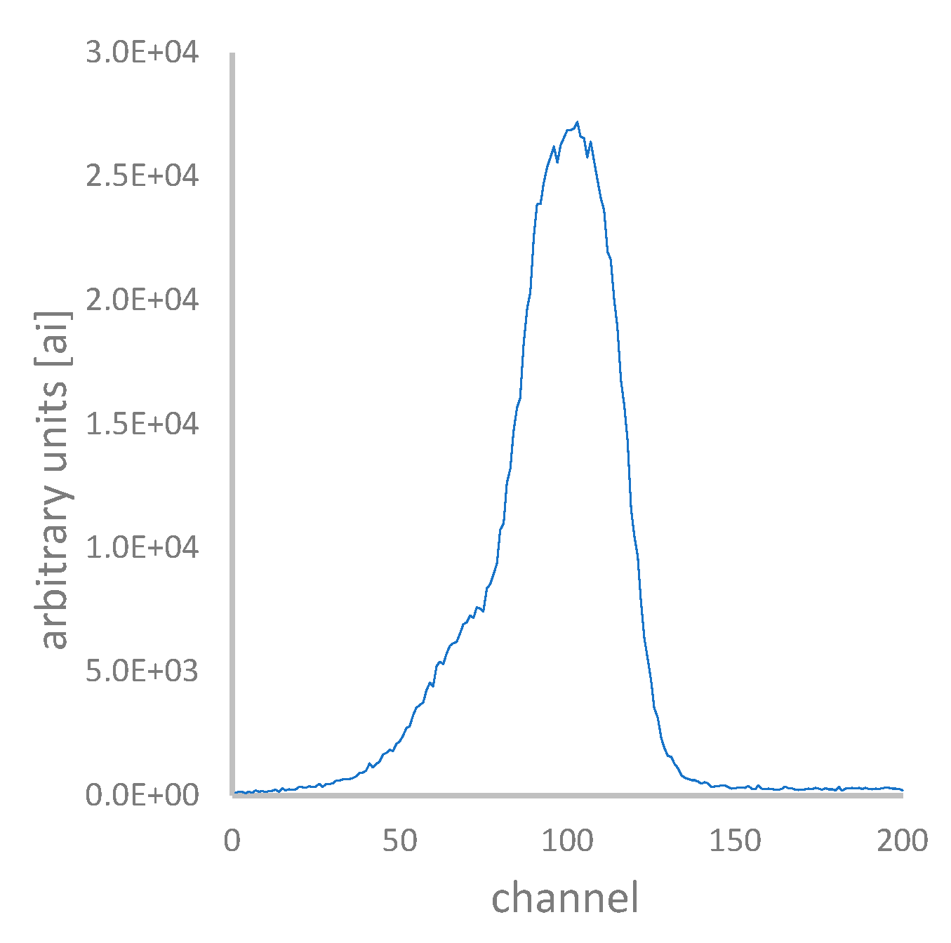
Figure 4.
Example of four glow curves, which were filtered out by the AI filter, which uses deep learning artificial neural network (ANN).
Figure 4.
Example of four glow curves, which were filtered out by the AI filter, which uses deep learning artificial neural network (ANN).
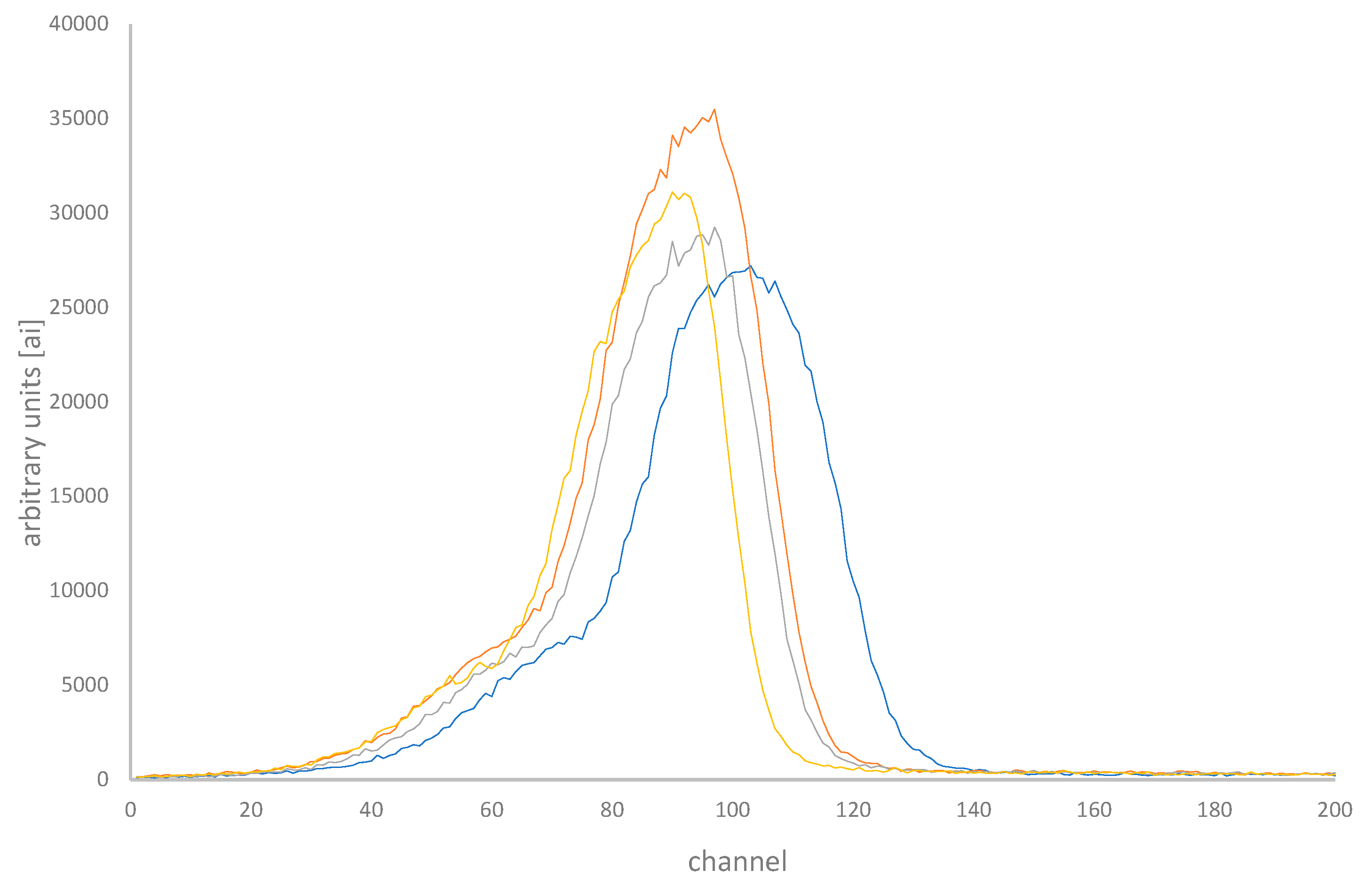
Figure 5.
A distribution example produced using the Qlikview BI helping tool. Out of the 97512 TLDs that were analyzed, 58550 were under the 16 mrem threshold. From the remaining 38962 TLDs, the AI filter found 7696 good TLDs, and the rest of them - 31266 dosimeters - were classified into the shown anomaly classes. Some of the TLDs can be simultaneously classified to both A Low and A High classes.
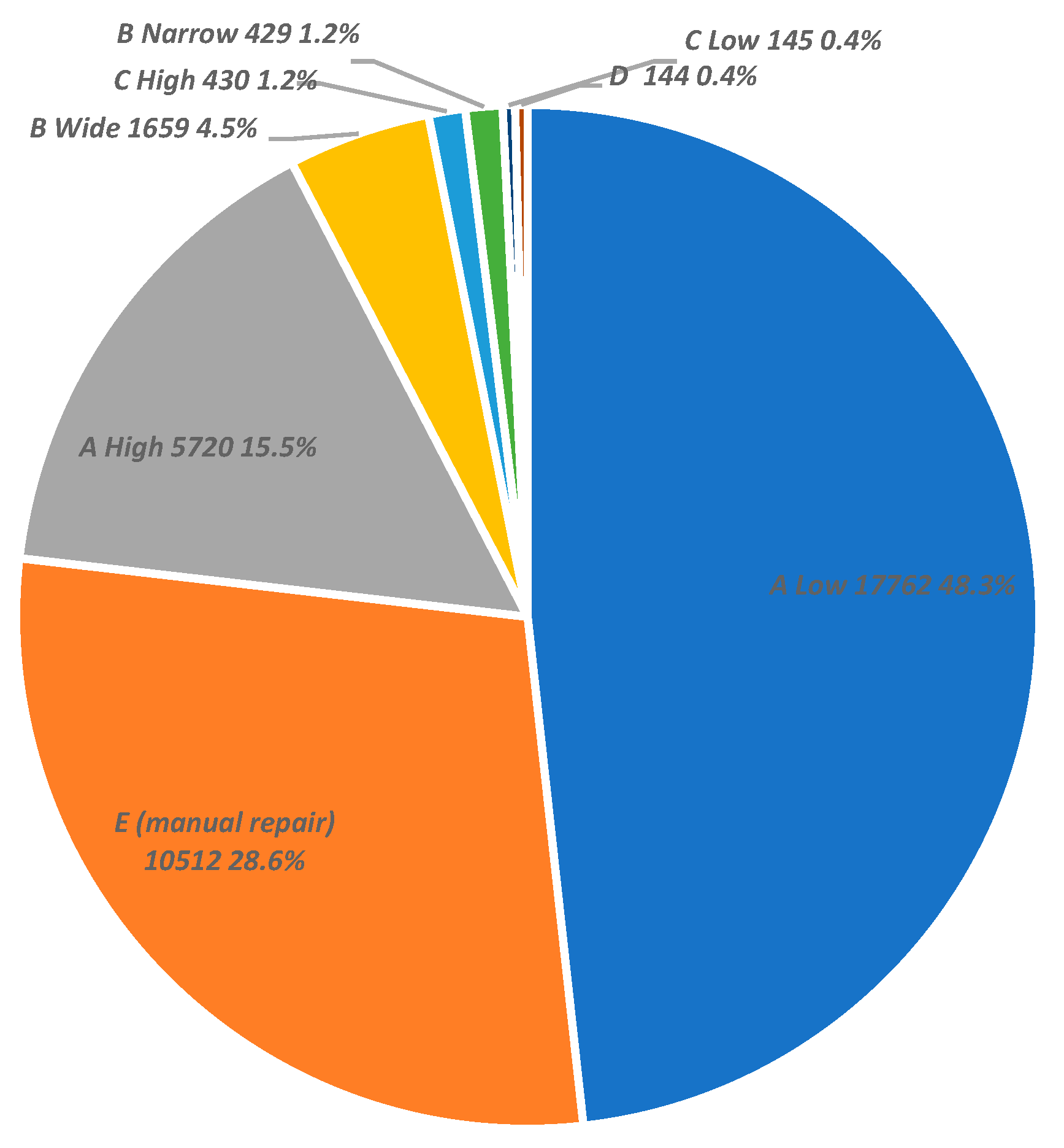

Table 1.
The different anomaly classes of the glow curves.
| Definition | Sub class | Anomaly class | |
|---|---|---|---|
| High background TL signal at low temperatures | Low | Class A | |
| High background TL signal at high temperatures | High | ||
| Invalid GC width – too wide GC | Wide | Class B | |
| Invalid GC width – too narrow GC | Narrow | ||
| GC shifted towards low temperatures | Low | Class C | |
| GC shifted towards high temperatures | High | ||
| Too many spikes | - | Class D |
Table 2.
All algorithm parameters inside the configuration ini file.
| Units | Description | Class / Module | Parameter name |
|---|---|---|---|
| mrem | Above this value, a dosimeter will be manually checked | General | ManualReviewThreshold |
| bool | Correct automatically without approval or not. | bFullAutomated | |
| mrem | Threshold under which 1st crystal is filtered out | Threshold1 | |
| Threshold under which 2nd crystal is filtered out | Threshold2 | ||
| Threshold under which 3rd crystal is filtered out | Threshold3 | ||
| Threshold under which neutron crystal is filtered out | ThresholdNeut | ||
| Threshold under which ring crystal is not checked | ThresholdRing | ||
| Weekly background | RadiationPerWeek | ||
| 0-1 | Ratio filter factor #1 | Crystals_Quotient | |
| 0-1 | Ratio filter factor #2 | ratio_table_threshold | |
| string | File path for winrems SQL data | MDBPath | |
| bool | Use AI filter | Machine Learning | bUseAI |
| - | ANN Model file name | training_model_file | |
| - | Above this threshold GC is classified normal | ai_probability_threshold | |
| % | Bgd max height relative to GC max height | Class A | MaxBgdHeight |
| Bgd min height relative to GC max height | MinBgdHeight | ||
| - | Minimal channel of high temperature | BgdHTTLChLow | |
| - | Maximal channel of high temperature | BgdHTTLChHigh | |
| - | Minimal channel of low temperature | BgdLTTLChLow | |
| - | Maximal channel of low temperature | BgdLTTLChHigh | |
| - | Max channel index for A_LTTL cut | LowCutCh | |
| - | Min channel index for A_HTTL cut | HighCutCh | |
| - | Minimal channel for width measure | Class B | TLDWideLowCh |
| - | Maximal channel for width measure | TLDWideHighCh | |
| % | Average height between minimal and maximal channels relative to max GC height | WideAvgVal | |
| - | Half width of narrow GC in # of channels unit | half_width_num_ch | |
| % | GC height relative to max height outside the narrow channels | NarrowAvgVal | |
| - | Max allowed shift from channel 95 | MaxAllowedShift | |
| - | Number of spikes found in GC | Class D | NSpikes |
| % | Percent difference between two neighbor channels | SpikeNeighDiff |
Table 3.
Integral ratio check table.
| L4/L3 | L3/L1 | L3/L2 | L1/L4 | E(keV) | Beam |
|---|---|---|---|---|---|
| 0.8 | 7.80 | 2.10 | 0.15 | 20 | NS 25 |
| 0.92 | 3.19 | 1.47 | 0.34 | 24 | NS30 |
| 0.95 | 1.50 | 1.15 | 0.70 | 33 | NS40 |
| 0.96 | 1.04 | 1.03 | 1.00 | 48 | NS60 |
| 0.97 | 0.94 | 0.99 | 1.09 | 65 | NS80 |
| 0.97 | 0.93 | 1.00 | 1.11 | 83 | NS100 |
| 0.98 | 0.96 | 1.00 | 1.06 | 100 | NS120 |
| 0.96 | 0.96 | 1.01 | 1.09 | 118 | NS150 |
| 0.98 | 0.94 | 1.01 | 1.09 | 164 | NS200 |
| 0.97 | 0.93 | 1.03 | 1.10 | 208 | NS250 |
| 0.97 | 0.89 | 0.97 | 1.16 | 250 | NS300 |
| 1.02 | 0.97 | 1.03 | 1.01 | 118 | H150 |
| 0.79 | 8.88 | 2.90 | 0.14 | 20 | M30 |
| 0.93 | 1.96 | 1.35 | 0.55 | 35 | M60 |
| 0.96 | 1.14 | 1.08 | 0.92 | 53 | M100 |
| 0.98 | 0.97 | 1.01 | 1.05 | 73 | M150 |
| 0.96 | 1.41 | 1.15 | 0.74 | 38 | S60 |
| 1.00 | 1.00 | 1.00 | 1.00 | 662 | Cs137 |
| 0.00 | 6200 | 6200 | 0.05 | Tl204 | |
| 0.30 | 4.98 | 67.5 | 0.68 | Sr90 / Y90 | |
| 0.23 | 6.44 | 24.2 | 0.69 | DU |
Disclaimer/Publisher’s Note: The statements, opinions and data contained in all publications are solely those of the individual author(s) and contributor(s) and not of MDPI and/or the editor(s). MDPI and/or the editor(s) disclaim responsibility for any injury to people or property resulting from any ideas, methods, instructions or products referred to in the content. |
© 2024 by the authors. Licensee MDPI, Basel, Switzerland. This article is an open access article distributed under the terms and conditions of the Creative Commons Attribution (CC BY) license (http://creativecommons.org/licenses/by/4.0/).
Copyright: This open access article is published under a Creative Commons CC BY 4.0 license, which permit the free download, distribution, and reuse, provided that the author and preprint are cited in any reuse.


