
Submitted:
08 November 2024
Posted:
08 November 2024
You are already at the latest version
Abstract
Consumer-grade economical radon monitors are becoming increasingly popular in private and institutional use, both in the context of Citizen Science and traditional research. Although originally designed for screening indoor radon levels in view of radon regulation and decisions about mitigation or remediation - motivated by the health hazard posed by high radon concentrations - researchers are increasingly exploring their potential in some environmental studies. For long time, radon has been used as a tracer for investigating atmospheric transport processes. This paper focuses on the RadonEye, currently the most sensitive among low-cost monitors available on the market, and specifically, its potential use for monitoring very low radon concentrations. It has two objectives: firstly, discussing issues of statistics of low count rates and secondly, analyzing radon concentration time series acquired with RadonEyes outdoors and in low-radon indoor spaces. Regarding the first objective, among other things, the inference of reported to expected true radon concentration is discussed. The second objective includes the application of autoregressive methods and fractal statistics to time series analysis. The overall result is that radon dynamics can be well captured using this "low-tech" approach. Statistical results are plausible; however, few results are available in the literature for comparison, particularly concerning fractal methods. The paper may therefore be seen as an incentive for further research in this direction.
Keywords:
Radon time series
; RadonEye
; counting statistics
; multifractal characterization
1. Introduction
1.1. Radon as Pollutant and as Tracer
Radon (Rn) is widely known as hazardous pollutant, which can cause lung cancer [1]. Consequently, there have been great efforts globally to monitor indoor Rn concentrations, assess levels of risk, and optimize Rn abatement policy and practice. As a direct result of these efforts there is now extensive national and international regulation of indoor Rn, e.g., the European Basic Safety Standards [2]. In recent decades the ever-present public health risk posed by Rn has resulted in the development of a wide variety of increasingly affordable and portable passive and active Rn monitors, e.g. [3,4,5,6,7,8,9,10,11,12].
Consequently, large databases of indoor and outdoor Rn measurements have been developed using these instruments, but (i) this data is not always easily available due to data protection issues, and (ii) the sensitivity and/or temporal resolution of these measurements may not be particularly high because reference levels for Rn are typically between 100 – 300 Bq m as annual mean.
But Rn also has a second face. Due to its unique collection of physical properties, the noble gas Rn can also serve as a convenient, efficient tracer in environmental studies of transport and mixing processes in the ground, hydrosphere and atmosphere [13,14,15]. One main technique in tracer research is the analysis of Rn concentration time series. Such studies seek to identify "signals" associated with some natural events and attempt to relate these signals to observed Rn variability. For atmospheric studies in particular, environmental Rn concentrations can be orders of magnitude below indoor or sub-surface radon concentrations, and exhibit variability on much shorter timescales (minutes to hours). These needs have driven the development of a separate collection of "direct" and "by progeny" active Rn detectors capable of measuring concentrations below 1 Bq m at sub-hourly temporal resolution (e.g., [16,17,18,19,20,21,22]). Large databases of outdoor Rn observations are now also being accumulated using these instruments associated with the WMO GAW and ICOS research networks. Unfortunately, it is not always possible to utilise outdoor Rn datasets collected by public health Rn monitors in the same ways as research grade environmental Rn monitors due to differences in sensitivity, precision, and temporal resolution. However, due to the much greater affordability of public health Rn monitors, there is value in increasing our understanding of their measurement performance in all settings.
1.2. Radon Source, Transport, and Temporal Variability
Environmental radon (Rn; here limited to the isotope Rn from the U decay series) has a predominantly terrestrial source. Rn emissions from ocean surfaces are typically 2-to-3 orders of magnitude less [23,24]. Its parent nuclide, Ra, is ubiquitous in soils, rocks, and most building materials. While the formation of Rn from Ra is relatively constant in time (Ra ∼1600 y), the release of Rn from soil grains, as well as its transport within and from the ground, is strongly influenced by changing soil moisture conditions and soil freezing [25,26,27]. Once Rn has entered the atmosphere, it is readily advected by wind. Because of the global Rn source heterogeneity, Rn’s 3.8 d half-life, and diurnally changing atmospheric mixing conditions, environmental Rn concentrations can show strong temporal variability which, in general, is difficult to model precisely. The reasons for this difficulty include missing - unavailable or unknown – predictors, and the overall high complexity of the "environmental Rn" system (see, e.g., the scheme "From rock to risk", [13]).
While Rn enters the atmosphere predominantly by diffusive transport, once in the atmosphere it is distributed by a combination of advective, turbulent and diffusive transport, depending on prevailing atmospheric conditions. In the absence of active convective clouds or strong fronts ([28,29]), Rn is essentially confined to the planetary boundary layer (PBL), the vertical extent of which is controlled at any given time by the combined total of convective and mechanical mixing processes. At night or early morning over land, when convective mixing is suppressed, the PBL depth can be quite shallow if wind speeds are light, resulting in higher Rn concentrations near the ground. When wind speeds increase, or daytime convection is active, the Rn concentration near the ground decreases due to dilution. The combined contributions of mechanical and convective turbulence at any given time dictate the atmospheric mixing state. One popular measure of the atmospheric mixing state (or stability) is the Richardson number, which is the ratio between buoyancy influences (driving convection) and the vertical wind speed gradient (driving mechanical mixing, in combination with the surface roughness). Diffusion of Rn in the atmosphere plays little role unless the atmosphere is very stable.
1.3. Low-Cost Radon Measurement and Citizen Science
Consumer grade radon monitors, which are orders of magnitude cheaper than professional "research grade" instruments, have become increasingly popular. To date, they have mainly been used in the context of private screening measurements and for Citizen Science. At the time of writing this article, the most sensitive among the consumer-grade radon monitors was the RadonEye monitor (FT Lab, South Korea [30]). Due to its economical price (less than 200€ for the basic version) it has become very popular and has been widely adopted by private and professional users, including use in Citizen Science projects. The RadonEye has been subjected to a number of QA studies (see section 2.1), the results of which appear favorable. Nevertheless, it is important to understand its limitations and define the objectives for its use. To this end, it is the intention of this study to scrutinize the performance of this monitor for a selection of indoor and outdoor applications.
1.4. Objective of the Paper
The objectives of this work are (1) to improve understanding of certain aspects of the counting statistics for results acquired by RadonEye monitors, and (2) to perform descriptive and exploratory statistics of indoor and outdoor Rn concentration timeseries collected using a RadonEye.
(1) The RadonEye only reports Rn concentrations in Bq m rounded to integers, leading to questions about the expected true concentration, conditional to the reported value. Since the exact algorithm used by the RadonEye is not publicly-available, we seek to better understand the reported results. Furthermore, we estimate detection limits and confidence intervals of the RadonEye count rates.
(2) We analyze indoor and outdoor Rn concentration timeseries recorded by RadonEye monitors over periods of several months. In addition to basic descriptive statistics, we apply autoregressive and fractal analysis, which has so far been less common in environmental radon studies. Tools are traditional time-series decomposition (analysis of trend and periodicity) and methods from the AR family (auto-regressive analysis). Further insight may be gained using multifractal methods such as the Hurst coefficient and spectra. The latter may help recovering long-term memory structures, which from a physics perspective reflect meteorological episodes (weather periods) rather than short-term variability.
The paper is organized as follows: the methods section has been split into two parts. The first part deals with measurement hardware and locations. The second part is about statistical procedures. This is followed by the results, with two sub-sections related to (1) and (2), above. Discussion of the findings and suggestions for further research are presented in the final section.
2. Methods 1: Hardware, Experimental Design and Data
2.1. The RadonEye Monitor
The instrument used to generate Rn time series is the RadonEye, based on an ionization chamber with sensitivity 1.35 cpm/(100 Bq m) = 0.81 cph/(Bq m) according to the manufacturer, or inversely, 1 cph corresponds to about 1.2 Bq m. It is not clear whether this is a generic value applied to all exemplars or a mean over individual calibration factors, and whether in each device the generic or an individual calibration is implemented. Its output are Rn concentrations which can be retrieved by smartphone app via Bluetooth. 10 min means are displayed but only 1 h-means rounded to integers are stored in a simple text file. QA studies - not to be discussed here in detail - show acceptable performance for usual indoor Rn concentrations [8,9] ; investigations with very low Rn concentrations (outdoors: typically <1 - 30 Bq m) are still missing. Problems seem to exist with sensitivity against Rn (thoron, Tn) [31] and dependence on humidity which may introduce bias, as well as with performance at extreme temperatures. Apparently for the latter reason the manufacturer does not recommend its use outdoors. Since the objective of this study is not the absolute value of Rn concentration but its dynamic, we shall not focus further on this possible problem. (However also the temporal behaviour may be impaired to some degree; this has however not yet been investigated.) One drawback is the lack of an internal buffer battery: in case of power loss the unsaved part of the recorded series is lost and a new series is started. Pictures of RadonEyes are shown in Figure 1.
Investigations concerning counting statistics and how to interpret reported results are presented in section 4.
Ionization chambers suffer from internal background (BG) due to the accumulation of the long-lived alpha emitting members of the Rn decay chain Po and Pb. Newly acquired devices, as used in this project, should therefore have very low internal BG. It seems that for new devices, one has to expect the equivalent of 1 Bq m or less (personal communication, BfS Berlin). This may be compared with sensitivity, 0.81 cph/(Bq m) or less than 1 count per hour (which is the reporting period) for exposure to 1 Bq m, which is common for outdoor Rn.
2.2. Measurement Locations and Periods
Vienna: Indoor radon concentration was measured hourly in Vienna, Austria, between 17 February and 23 July 2024. The monitor was placed on a rack near a bookshelf about 50 cm above the wooden floor. The room is located on the second floor of an apartment building built in the late 19th or early 20th century, made of brick, typical for Vienna. The building has four floors plus a basement whose floor is not isolated against the ground and which is also not isolated from the interior of the building. The room is about 3.6 m high and has an area of about 20 m. Two windows look onto a courtyard; their wooden frames are quite old and, in spite of double glass, they are not very airtight. The local geology is Holocene alluvial of the Danube [32] with low geogenic radon potential. Previous measurements in the same room (19 August to 12 November 2000) using a Pylon-AB4 monitor (based on Lucas cell) consisting of 2093 hourly means (as for the present analysis) yielded a mean Rn concentration of 15 Bq m only (min-max = 0 - 46). However, windows were open during part of the measurement period. If the windows were closed, the concentration rose to about twice as high, indicating influence of either geogenic Rn or exhalation from building material. Another 2-week trial measurement by RadonEye in April 2023 gave 30 Bq m (windows closed). The location is 48.22° N latitude / 16.37° E longitude.
Berlin: Outdoor Rn was measured in Berlin, Germany between 23 February and 29 July 2024. The monitor was placed in a protective plastic case Figure (Figure 1) on a wooden balcony about 2 m away from the wall and about 6 m above ground, a large garden. The ground is post-Weichsel glacial alluvial of the Spree Urstromtal [33], mainly sand, with low geogenic radon potential. Long-term measurement using track-etch passive detectors at a nearby location, 1.5 m above ground, gave a 3-year-mean outdoor concentration of 6 Bq m[34]. Four test measurement series with RadonEye in May, July/August, September and October 2023 gave 3, 3, 7 and 6 Bq m, respectively.
Berlin: Indoor Rn: Two indoor Rn series were recorded in Berlin. The first between 25 October 2023 and 3 February 2024. In the same apartment, radon has been measured indoors partly in parallel with outdoor Rn between 2 June and 29 July 2024. The RadonEye was placed like shown in Figure 1, left, during the first (winter) period and in a plastic box open upwards, located nearby directly on the tile floor, during the second (summer) period. Possible thoron influence is probably negligible. During measurement, windows were mostly closed. The apartment is located below the wooden roof (corresponding second floor) of a building about 90-100 years old. There is a souterrain-type basement with concrete floor, normally separated from the interior of the house by a locked, but not air tight door. The location is 52.49 N latitude / 13.53 E longitude.
3. Methods 2: Statistical Analysis of Reported Rn Time Series
Basic methods (descriptive and exploratory statistics, periodogram) follow established rules and will not be discussed here. This section is concerned with the interpretation of the reported results, not with measurement statistics. This is discussed in Section 4.
3.1. Box-Jenkins Scheme
3.1.1. Autoregressive Moving Average Model
This procedure attempts to separate variability components of a time series, test for the presence of a trend, adjust the series by removing trend and periodicity thus identify aperiodic variability. Further it helps estimating an autoregressive model that allows prediction. Thus, the residuals about the model can be traced to the aperiodic components. The most comprehensive textbook is [35]. For a short introduction, e.g., [36], the NIST handbook [37], section 6.4.4.5 and the Wikipedia entry "Box–Jenkins method". Time series are conceived as realizations of autoregressive (AR) processes,
or moving average (MA) processes,
where are random terms associated to the i-th member of the series; thus the value at t is influenced by the noise of pdimension revious terms. The highest index of and is the order of the process. AR and AM are combined to ARMA() processes, p and q the AR and MA orders. The concept is extended to ARIMA() or autoregressive integrated moving average process. The order d can be fractional (F), resulting in ARFIMA or FARIMA [38] models. The parameter d refers to differencing the original series, , repeated d times (fractional d require particular definition), and applying the ARMA procedure to Y. For application of the ARFIMA technique to Rn series, see [39]. Differencing X is performed if the original series is non-stationary. The technique is much used in financial mathematics, in climatology and other disciplines which deal with time series, but less so in the field of Rn. As one notable paper we mention Stransky [40], who applied ARIMA with external (exogenous) predictors to a Rn time series recorded in a cave.
3.1.2. Box-Jenkins Scheme - Autocorrelation and Partial Autocorrelation Functions (ACF and PACF)
Analysis of the ACF and PACF enables estimation of the model structure in terms of AR and AM order. The PACF removes the influence of correlations for each preceding lag., see [35], section 3.2.5. How this is done to estimate the orders of ARMA() will be shown in the results Section 5.2.2.
The correlation length, that is the period during which the values are considered correlated, can be quantified by the time after which the correlation decreases below a threshold. Commonly used ones are or as error probability of the null hypothesis: "not correlated".
3.2. Stationarity
Stationarity is a rather tricky concept and there are different definitions and approaches. A stochastic process X is called stationary if . Another definition is for all t, that is, time shift does not change the expectation. In general this cannot be proved because usually one has only one realization of X, so that the about equivalent Birkhof-ergodicity, loosely put cannot be tested ( - index that counts realizations of process X). Finding a trend within a limited domain (the observation time or space) does not indicate non-stationarity because in a larger domain the picture may be different. For example, the indoor Rn series in Berlin both look about stationary, but they are different between winter and summer, indicating an annual cycle (which exists as is known from other experiments). But extending the series over many years would again let appear it stationary. Non-stationarity would be given if for some physical reason, such as climatic change, there would be a long-term increasing or falling trend; but such effect has so far not been identified. For the purpose of our analysis we may assume the series stationary. A non-decaying ACF indicates that the series is probably non-stationary in the investigated domain.
To complicate further, stationarity and stationarity on top of a trend has to be distinguished. In the latter case the presence of a deterministic trend is assumed, around which the series fluctuates. The question is whether this fluctuation is random walk-type, i.e. non stationary.
In spite of the assumption of stationarity based on underlying physics, some statistical tests were applied.
The non-parametric Mann-Kendall test [41] (see also the Past4 manual) looks for a deterministic trend in the series. The Dickey-Fuller stationarity test [42] is based on differenced series; it tests whether coefficients of differences are equal 1, therefore it belongs to so-called unit root tests. the p-value of the 0-hypothesis root=1 is determined, which indicates non-stationarity. Here the basic and the augmented versions of the test as implemented in Gretl [43] were used.
3.3. Multifractal Methods
Fractal and multifractal aim to explore the "irregular" behaviour of a field or a time series, that is the variability beyond trend and periodicity. This manifests in non-periodic "episodes" of higher or lower values of the response variable (here, Rn concentration) and in the "roughness" of the series graph.
3.3.1. Hurst Coefficient
The term Long Memory "refers to persisting correlation between distant observations in a time series" [44], excluding correlation due to periodicity. Long memory indicates the presence of aperiodic episodes in the time series, typical for Rn series, owing to weather episodes as meteorology is the most important predictor. If one succeeds to explain the episodes in the Rn series from meteorological episodes, the remaining unexplained variability indicates the presence of additional predictors not accounted for. Many authors attempted to use signals in ground and hydrological Rn time series for seismic prediction because it is empirically known that seismic / tectonic phenomena can produce Rn signals. However, no reliable seismic prediction based on Rn has yet been successful, if one understands acceptably low first and second kind prediction error probabilities as criterion of reliability.
The Hurst coefficient is a measure of persistence, or the tendency that the variable approximately maintains a certain level for some time. 0.5<H<1, with higher H meaning less volatile or smoother series. High (low) values tend to be followed by high (low) values, which can be interpreted by (irregularly) recurring "episodes" which last some time. H<0.5 indicates an anti-persistent process, meaning that values tend to change quickly between low and high. H=0.5 indicates Brownian motion. Bowers & Tung [38] cite a number of physical phenomena for which long-term dependence has been found. An interesting paper of the history of the Hurst effect is Graves [45], which also discusses the connection with ARFIMA.
3.3.2. Multifractal Spectrum
Multifractals can be understood as interwoven fractals of point sets which are realizations of random fields, where an "intensity" is given at locations of the carrier domain (here: the time axis). This can be understood as the density of a measure (in the mathematical sense) within a "box" (time interval) of given size h. It is assumed that locally, the field behaves as , where is called the local Hölder exponent or singularity strength at location t. The number of boxes with Hölder exponent behaves as , and the graph is called multifractal spectrum. It looks like an upside down parabola which is the wider, the "rougher" the graph of the time series is (The same applies to spatial fields). The dimension for high characterizes the pattern of extremes of Y, in this case the Rn concentration. For rigid definitions and a more detailed discussion see, e.g., [50,51] or the textbook [52].
3.3.3. Fractal Dimension of the Graph
The graph interpreted as a point set has a fractal dimension D which measures its "roughness". Among infinitely many possible definitions of D usually the box dimension is chosen in this context. Essentially, the graph space , with embedding Euclidean dimension 2 in our case is divided into equal boxes and the number of boxes "occupied" by points of the graph is counted in dependence of box size or scale. The number scales like where the scale is the box size relative to some initial size or as a fraction of the area of the entire domain. D can therefore be estimated as slope of the plot. By theory, , with 2 = the embedding dimension of a time series graph.
For analyses related to Rn, see [47] who found good agreement between estimations of D via box counting and the Hurst coefficient.
3.3.4. Garger Exponent
Garger et al. [54] investigated the fluctuation of radionuclide concentrations in aerosols after the Chernobyl accident (1986). They found a power law dependence of the fluctuation over a period from this time, , for not too long aggregation periods T. They found which would coincide with what one expects for turbulent wind fields. The approach was further elaborated by Hatano et al. [55,56]. Smooth functions would yield , white noise, and random walk, . Concerning Rn, the coefficient was first calculated in 2002 [57] for the several indoor Rn series, resulting quite consistently in g = 0.60 - 0.62.
is defined, with over series of length T.
3.3.5. Attractor Embedding Dimension
The phase space of the process can be reconstructed from the time series with an algorithm based on Taken’s embedding theorem; see [58] sec.5 and for an easy explanation, e.g., [59,60]. From the time series , i = 1...n, we construct the E-dimensional series , where E is the Euclidean embedding dimension and a time delay which has to be chosen appropriately that and are little correlated. A reasonable choice of is the decorrelation time according to the ACF. The embedding dimension E can be seen as estimate of the number of variables which control the system.
Estimation of the minimal E is performed with two methods: (1) in the y-space, which is topologically equivalent to the phase space, the correlation dimension is determined: For every , one counts the number N of points within distance . The mean scales as , so that can be estimated as slope of the plot. The correct E is found when levels off with increasing E. (2) In the false nearest neighbor (FNN) technique one chooses E such as to minimize the number of so-called false near neighbors, which are points of the y-series which falsely appear as neighbors of due to E set too small. One increases E until the FNN rate is reasonably low.
3.3.6. Lyapunov Exponent
A qualitative definition is given in [64]: "The Lyapunov exponent (...) is (...) the measure of the sensitivity of a system to its initial conditions. Lyapunov exponents (...) are related to the exponentially fast divergence or convergence of nearby orbits in phase space. A positive Lyapunov exponent is an indication of chaotic behaviour in the time series, while a negative value of Lyapunov exponent shows periodic trajectories, or non-chaotic behaviour, of a dynamical system. The more positive the value of Lyapunov exponent is, the shorter is the time interval up to which the system’s future can be predicted and vice versa." Nearby orbits or trajectories are followed with time and their separation is measured. The maximal Lyapunov exponent is the rate of an anticipated exponentially growing separation. In [57] estimation of Lyapunov exponents together with phase space reconstruction through the recurrence plot technique, introduced by [56] and much used since, have been attempted, but little further literature in the field of Rn studies exists, quoted in the results section.
Software: basic operations and graphs were produced with Excel; for time series analysis, Past v. 4.03 and 4.17 [65], Statgraphics v.4 and Gretl 2019a [43], CDA 1.1 [66] and different R packages were used, detailed in the respective results sections. The Hurst exponent, the spectra were additionally computed with in-house developed software written in QB64 [67].
4. Results 1: Aspects of Counting Statistics
Basic properties of the RadonEye monitor were presented in Section 2.1. In this section, we shall address some issues related to low count rates and to the (unknown) internal evaluation algorithm of the device.
4.1. Critical Limits
The simple Currie approach [68,69] gives , . With usual 1-sided = 1.645, this is and For the newer ISO 11929 version, which yields slightly different values see, e.g., [70,71,72]. Here we stick with the Currie version for simplicity.
Assuming a BG of 1 count per hour, BG=1, we find = 2.3 counts = 2.9 Bq m and = 7.4 counts = 9.1 Bq m. On the other hand, in many instances 0 or a few Bq m are reported; even if BG=1 may be too high for new RadonEyes, this shows that very low reported values should be understood cum grano salis. Dependence of the critical limits on BG is shown in Figure 2.
4.2. Frequentist Poisson Confidence Interval of Counts
The device counts pulses and its uncertainty can therefore be estimated from Poisson statistics. Figure 3a shows the dependence of relative uncertainty on concentration, for three measurement periods, under the Poisson hypothesis and the sensitivity reported by the manufacturer. Confidence intervals can be calculated by different methods, summarized in [73]. We prefer the simple . Here is the inverse Chi-square with and degrees of freedom, respectively, x the count number. The (i.e., 95%) - confidence limits for low count numbers are shown in Figure 3b. For x=0, CI95%=(0, 3.7), for x=1:(0.025, 5.6), x=2:(0.24, 7.2), and so on.
The often used Wald interval , based on the normal approximation of the Poisson distribution, is applicable only for high observed counts x, say x>15. The reasoning would become more complicated if considering the BG.
In its smartphone App, the RadonEye reports a 95% confidence interval for the last one hour measurement based on six 10-min counting periods. The algorithm is not publicly available. For nominal 0 Bq m, a CI = (0, 19) is given, which appears too large to me if compared to the above estimate.
4.3. Bayesian Estimate of the Expected True Count Rate
We assume as prior the conjugate distribution of the Poisson distribution, which is the gamma distribution, (see, e.g., [74] or the Wikipedia entry "Poisson distribution". The predictive posterior distribution (i.e. the distribution of x) is the negative binomial. The posterior Poisson mean for n=1, the number of observed counts of size x. We guess and such that the gamma (i.e. the prior) mean equals the midpoint of the frequentist confidence interval. Since Poisson variance = mean we find =1 and =midpoint; however Bayesian inference has it that this choice is to an extent deliberate and may be understood as reflecting plausibility. is shown in Figure 3b. With the Bayesian mean approaches the observed count number x. For x=0 observed counts, the estimated mean equals 0.92, for 1 count, m=1.9, and so on.
4.4. Bayesian Inversion of Reported Rounded Concentration Values
The RadonEye reports Rn concentrations rounded to integers, , - calibration factor (cph/(Bq m)), k - counts per period T, in different notation; therefore, re-converting into counts introduces additional uncertainty, . The actual rounding algorithm used in the RadonEye is not publicly available (For further information on the various rounding algorithms, please refer to e.g. the Wikipedia entry on "rounding").
The question is therefore, given a concentration C (rounded to integer) reported by the instrument, which is the expected true concentration or its most probable value (or more generally, its distribution)?
Let the true mean concentration in interval T (here we focus on T=1 hour. In reality, Rn concentration is not entirely constant during one hour, see Figure 7, but considering this would render the reasoning very complicated. This may be left to a future study). In the following, the results refer to interval T. The index T is therefore suppressed.
C(true) leads to a number of pulses k within interval T. These are Poisson distributed with mean , that is, . The probability to count k pulses is
The registered concentration and reported concentration, . Some example values of for true concentrations between 0.5 and 4.5 Bq m are shown in Table 1. For instance, if the true concentration is 2.5 Bq m (first row), the RadonEye reports 6 Bq m (third column) with probability 3.7%. This table will be inverted in the next step.
can be interpreted as conditional probability . The wanted posterior probability , which is the probability that the true concentration is if - an integer number - is reported by the instrument, is therefore, by Bayes Law:
For the prior we can choose a constant as an improper uninformative prior, so that it cancels in the numerator and denominator, and the desired posterior can readily be computed. Among many other possibilities, a sufficiently wide rectangular function centered around could also be chosen as a prior. (Of course, the estimated posterior always depends on the choice of prior to some extent.) From the posterior distribution, the conditional mean, the most probable value of the true concentration, and other statistics can be derived. Here, the calculation was done with a custom QBasic program.
The result using the improper-uninformative prior is shown in Figure 4. The most probable true concentration is practically the same as the reported. The expected true concentration is somewhat higher but the relative distance decreasing (lower right inset).
Re-converting the expected true concentration into counts and comparing with observed counts shows, like in the previous section, a decreasing difference (upper inset of Figure 4). Comparison with the more formal derivation in Section 4.3 shows very little difference. For observed x=0 and x=1 counts, the expected values equal 1.06 and 2.04, respectively, to be compared with 0.92 and 1.9.
4.5. Missing Nominal Concentration Values
Rounding induces a rather strange effect, namely, that certain integer values of can never occur, see Figure 5, for two values of cal and also in Table 1, third column. For cal=0.81 (default for the RadonEye), = 3, 8, 13,... Bq m cannot occur. For cal=0.79, this would be =2, 7, 12,.. Empirically, for three investigated RadonEyes missing nominal concentration values given in Table 2 are observed. We can see that 1) the missing values are different between the devices and 2) that the sequences are not regular as they should be if the proposed explanation is sufficient. Evidently it is not, although it is probably the core of the problem. A satisfactory explanation should be given by the manufacturer.
As a summary of the preceding sections, several open problems remain to be solved before the findings can be implemented in practice. However, only the manufacturer can provide detailed information about the algorithm. Therefore, the subsequent analyses of the empirical time series will rely on the reported raw data. The error is likely not significant, as the Bayes-expected concentrations, conditioned on the raw data, do not differ substantially from the raw values, except for concentrations close to zero. Moreover, this paper focuses more on the dynamic patterns of the series rather than absolute values, so a potential bias in these values should not significantly affect the results.
5. Results 2: Descriptive and Exploratory Statistics
5.1. Descriptive Statistics, Periodicity And Autocorrelation
5.1.1. Time Series and Descriptive Statistics
Table 3 presents basic statistics of the radon series graphically shown in Figure 6. The maxima observed in Berlin (indoor) about end January 2024 and Vienna end March / early April 2024 coincide with Sahara dust episodes. To our knowledge, the exact physical reason has not yet been explored. We hypothesize that Southern wind implies that air travels longer distances above territories with higher geogenic Rn exhalation than Westerly winds (predominant in Vienna and Berlin) that origin over the Atlantic Ocean. The short 10-day outdoor series recorded during a very hot period in mid-August 2024, Figure 7, shows the high diurnal variability, and that the maxima occur during morning hours. Low concentration values should be understood subject to Section 4.3 and Section 4.4.
5.1.2. Stationarity
The Mann-Kendall test for trend (performed with Past 4.04 because the more recent version 4.17 seems to have an issue with this test) indicates presence of a significant trend for all series. This may however be an accidental effect particular to the chosen measurement periods. According to the simple as well to the (stronger) augmented Dickey-Fuller test performed with Gretl, all series are approximately stationary at p<0.05 if the presence of a trend is considered.
5.1.3. Periodicity and Autocorrelation
Periodicity and autocorrelation (the ACF, autocorrelation function; the PACF - partial autocorrelation function - is discussed in Section 5.2) are summarized in Table 4 and visualized in Figure 8. The periodograms show the expected 24 h periodicity. In addition, one can recognize periodicities whose physical origin is unclear. The one of 26 - 27 days may point to lunar tides, although the synodic lunar period (time between the same phases of the moon) equals 29.53 days, the sidereal period (same position relative to the stars), 27.32 days. The other periodicities may reflect meteorological patterns: Periods of persistent inversion in winter and hot periods in summer with little wind and low turbulence are common in Central Europe (see, e.g., the several week long heat periods in summer 2024, interrupted only by rainy and stormy days which last few days, and the likewise week long notoriously depressing grey and cold inversion periods in winter). The diffuse clusters of periodicities around 3 days and 10 days may refer to such patterns. Similar interpretations were reported by Kikaj et al. [75]. The slope of the log-log periodogram for small frequencies refers to the model: , indicating the presence of coloured noise, see Section 5.3. For high frequencies, the periodograms show a flattening of the power with frequency, recognizable from the graphs in frequency domain (inset in the graph Figure 8, upper). In this range (temporal resolution of 10 h and below) the periodogram indicates that the reported data tends progressively to white noise. The probable reason is instrumental noise. This has also been found in [57] and in the TraceRadon project [76].
The autocorrelation plots show that in Vienna Rn reacts more slowly to external drivers than in Berlin indoors during the summer period, but similarly to Berlin indoors in winter (series Berlin-in 1). For some reason yet to be explained, indoor Rn dynamic in Berlin is different between the winter and summer periods: in winter the daily period is much less pronounced than in summer. Mean Rn concentration is higher in winter than in summer - a typical effect, perhaps due the stack effect induced by heating. This may also explain why it reacts to outdoor conditions less than in summer. Autocorrelation decreases very fast from lag 0 to lag 1, which "nugget effect" is due to the high statistical uncertainty of the values.
5.1.4. Cross-Correlation Indoor-Outdoor Radon
Cross-correlation analysis between the outdoor and indoor (summer) series shows that in Berlin, outdoor Rn is 6 hours ahead of indoor Rn (series 2) in average (Figure 9). The low overall correlation is due to the very high uncertainty of low Rn concentration values below decision and detection limit, see Section 2.1. Nevertheless, the Fourier and autocorrelation analyses indicate that the dynamic pattern of Rn concentration is adequately represented, despite the potential for uncertainty regarding the reported low values. It is important to note that the lag of 6 hours (lag=6h) represents an average value, which may not be constant over the entire period.
The ratio between outdoor and indoor Rn concentration in Berlin during the period when the monitors were working in parallel is shown in Figure 10. The 6-h lag has been considered. The plotted values are the ratios between means in 24-h sliding windows. The anomalous peak towards the end of July is not explained. The apartment was not occupied and windows were closed during the entire period. The mean ratio is equal to 0.39, which can be interpreted that outdoor Rn contributed about 39% to indoor Rn during that period. The remaining is owed to geogenic Rn and in a minor part to the (probably very little) exhalation from building material. Exhalation from water can be excluded during that period.
5.1.5. Outdoor Radon Diurnal Pattern
Accounting for the main 24-hour periodicity, outdoor concentration values were aggregated per hour of the day in Figure 11. One can clearly recognize the nocturnal radon accumulation effect which leads to maxima at 5 in the morning and minima around middle afternoon, in average. The physical reason is the higher atmospheric stability at night which leads to lower atmospheric mixing layer height and resulting higher Rn concentration. Similar graphs are shown in [77,78,79,80,81], or [76] Figure 15, p.44 for the EEC. An extensive study of these patterns is presesnted in [82]. The time of the maximum and the onset of increasing and decreasing depends on sunshine hours. The series was recorded between February and July in Berlin, where sunrise varies between 7:05 and 4:20 CET in the morning during the measurement period, so that the curve is "smeared" as reflecting this variability. This is corroborated by Figure 12, which shows the same curve for the measurement months: one can notice that in tendency, the maxima and onsets shift to earlier and later hours, respectively, with increasing month. Kikaj et al. [83] Figure2, have shown that the actual shape of the diurnal Rn concentration curve depends on atmospheric mixing classes; however our data are not sufficient to repeat the analysis for our location.
For Figure 13, the maxima were filtered. For every , we compute AM9(t) := AM[x(t-4),...,x(t),...,x(t+4)], that is, the 9-hour mean around x(t) leaving out x(t); then, considering that the Poisson SD equals , set a 2 sigma threshold ; and finally, if the hour of the day is between 1 and 8 in the morning and x(t)>th, retaining x(t). One can recognize in Figure 13 that the maxima vary aperiodic considerably, with some weeks with low and some weeks with high maxima.
5.2. Autoregressive Modelling
5.2.1. Simple ARMA
Table 5 shows the AR and AM coefficients of the time series estimated with the ARMA module of Past software. The model has been optimized by the by minimizing the AIC (Akaike information criterion). Figure 14 show the original, modelled and residual series for Vienna (residual = original - model). Perhaps 5 AR components would not really be necessary, as already an ARMA(1,1) model has AIC=2.589e4, that is, the additional autoregressive coefficients improve the model only little. Introducing a differencing step, ARIMA(p,1,1), does not lead to improvement. On the other hand, the difference series x(t)-x(t+24), which largely removes the diurnal cycle, leads to ARMA(1,1) with lower AIC=2.816e4. The model performance may be compared between the series by computing the mean square of the relative residual, defined here as . We see that the models for the indoor series perform similarly, the one for the outdoor series a bit worse. In the absence of comparable results from the literature we cannot interpret the result in relation to Rn series recorded elsewhere.
5.2.2. Partial Autocorrelation
The shape of the partial autocorrelation function (PACF) informs about the order of the autoregressive model as the number of significant lags. Figure 15 shows the ACF and PACF of the Viennese series. The number of significant PACF lags, 4 to 5, coincides with above findings (Table 5), corroborated also with Gretl software. First order differencing or introducing an ARIMA order d>0 does not improve the model but suggests the presence of one AM component, as also found above (Table 5). For the series: Berlin-out, Berlin-in1 and Berlin-in2, one estimates 4, 7 to 8 and 3 AR components, respectively, slightly different from the findings above. The 7 to 8 AR components suggested for Berlin-in1 from the PACF are also not confirmed by the ARMA analyses of Gretl which suggests 1 to 2 AR components.
5.3. Fractal Analysis
Several authors have applied fractal methods to explore the dynamic of Rn time series. While estimation of the Hurst exponent has led to consistent results, in most cases, other statistics have been less studied and often led to questionable results. For example, [84] applied fractal methods to Rn emissions from a mud volcano in Italy, demonstrating methodology but without conclusive results.
5.3.1. Hurst Exponent
The R/S graph from which the Hurst exponent is derived by log-log linear fitting, is shown in Figure 16 as example for the Vienna series.
In a previous study [57], for the same apartment in Vienna, H=0.92 was found, using an adapted R/S method. The same study reports 0.74-0.92 for different rooms of a house in Salzburg. For outdoor Rn, [85] found H=0.81. A similar list is given in Donner [49]. In a number of studies mainly on indoor and soil Rn series, similar H values were found, indicating persistence and long memory, as could be expected by weather episodes that last typically some days and which are the drivers of aperiodic Rn variability. As three more examples, [86] found H=0.70 – 0.85 for indoor Rn series, [71], H=0.88 and [87], up to 0.9. For Rn exhalation from uranium tailings, [88] found H=0.80. In a study aimed to search for seismic signals in soil Rn time series, [89] found H=0.7-1.
However, there are also studies cited in [85] that found H<0.5, for example [90], opposed to our own study and the ones quoted above. This is implausible on physical grounds and could be caused by erroneous software. Older versions of CDA, such as the freely available v.1.1 from 1995, appear to yield systematically low H values. While a more recent version (v.2.2) is documented in [74], its high cost has limited testing and verification of potential improvements. CDA v.1.1. can be run under DosBox on Window 7 but certain functions are very slow. Table 6 shows Hurst coefficients of the four series estimated with different software and algorithms. Finally, the function ’hurstexp’ in the R package ’pracma’ [91] was used which gives different outputs based on different methods. For both, a large minimum box size was specified. Two are given in Table 6. In spite of a consistent tendency, the differences show that exact estimation seems not to be trivial. Some issues of estimation of the Hurst exponent are discussed in [92].
5.3.2. Multifractal Spectra
The spectra of the four Rn series are shown in Figure 17. The parabolic shape is as expected; slight deviation from strictly parabolic may point to deviation from multi-fractality. The aperture of the parabolas is different, with the outdoor series showing the highest spread between and . This points to particularly pronounced "anomalies" (maxima) while the indoor series are comparatively "smoother". This is plausible from a physics perspective because the indoor space serves as a smoother of the dynamic. So far we are not aware of spectra of Rn series reported in the literature, therefore we cannot compare our results with the ones of other authors.
5.3.3. Graph Dimension
The box dimensions D sub B of the four time series are listed in Table 6 together with the derived Hurst exponents. The values coincide more or less; in particular for the Berlin outdoor series we recognize a discrepancy whose source is not known. The graphs from which the DB are determined by regression are shown in Figure 18. The values were calculated with the sliding box method, where rectangles of sizes corresponding to the scale are moved over the 2-dim graph space and the rectangles counted which contain points of the graph, that is the number of non-empty boxes which cover the space.
5.3.4. Garger Exponent
The graph from which the exponents g are determined by linear regression is shown in Figure 19. The used range is h. The resulting exponents (Table 7) are 0.66 - 0.78 for the indoor and 0.79 for the outdoor series. The exponent of the Viennese series is similar to the one found in [57] for the same room years ago. The series fluctuate more strongly than expected for turbulent flow (g=0.33), but less than white noise (g=1). Outdoor Rn seems to be noisier than indoor Rn, which is physically plausible.
5.3.5. Attractor Embedding Dimension and Lyapunov Exponent
According to Eckmann [93] the highest minimal E that can be reasonably estimated equals approximately 2 lg N, with N the length of the time series. For the Viennese, Berlin outdoor and Berlin indoor-1 series, this implies , for the shorter series Berlin indoor 2, .
With CDA 1.1 software, the minimal embedding dimension E can be estimated with the plateau of the correlation dimension versus E or with the false nearest neighbour (FNN) statistic. Delay times were chosen according to the ACF, i.e., the time after which the ACF is close to zero (Table 8). Additionally a standard =16 h was used; the results are not very different. They are summarized in Table 8 for according to the ACF. Note that CDA allows setting only in powers of 2. For comparison, in [57], E = 4 to 6 were found. CDA has a module for the Lyapunov exponent, but this does not work under CDA in DosBox. Screen shots of CDA outputs are shown in Figure 20 for Berlin indoor 1 and Vienna.
With R, packages ‘tseriesChaos’ [61] and ‘nonlinearTseries’ [62], we found the following results. Some of the used functions require extensive parameter setting, which was partially done by trial and error.
In the package ’tseriesChaos’, E was estimated with the function ’false.nearest’, the maximal Lyapunov exponent L with ’’ and ’lyap’. For the delay , the values according to the ACF close to zero and the value where the first minimum of the ACF occurs were used. Results are not too different. In the package ’nonlinearTseries’, the ’estimateEmbeddingDim’ was used, based on the Cao method [94]; but no plausible or interpretable results could be found, mostly because E was estimated too high, that is . For the Lyapunov exponent, the ‘maxLyapunov’ function was used. In all cases, model parameter such as minimal search vicinity and Theiler window (to exclude spurious neighbours) were varied until some plausible result was achieved. (This does not appear very satisfying, but seems to be common practice when analyzing real-world time series.) The function does not give uncertainties or confidence intervals of L, nor p-values to test against the null hypothesis L=0; but from visual impression of the S versus t graphs (S – the separation of phase space points, t – the time along the trajectories from some starting point; graphs not shown here) the values given in Table 9 do not appear significant.
Evidently there is a discrepancy between L values computed with different programs. The low maximal Lyapunov exponents indicate low degree of chaotic behaviour of the series. However, estimation is difficult and results should not be taken too literally, in particular in the absence of much literature results to compare.
We also tried the R package ’DChaos’ [95] but this did not appear successful, yielding consistently negative L; however, these seem to by typical for periodic series. Perhaps the algorithm identified this effect. Further, the software GChaos [96] seems to be user friendly and offers good functionality, but lacks documentation. It applies three algorithms for the Lyaponov exponent, with two methods yielding values around 0.005, one method, values ten times higher.
Planicic et al. [90] reported Lyapunov exponents of hourly sampled outdoor Rn data about ten times higher than the ones of ‘tseriesChaos’, but similar to ones found with ‘nonlinearTseries’. Similarly, Glushkov et al. [97] found maximal L = 0.018 for outdoor Rn. Bossew et al. [57] found values between 0.08 and 0.14 for indoor series.
As a conclusion of this section, stable estimation of the Lyapunov exponent of the time series of this study has not been satisfactory and further investigation is required, including diving deeper into the mathematical and computational details of the algorithms.
6. Conclusions
Although hourly measurement values for low Rn concentrations recorded with the RadonEye monitor have high uncertainty and are often below the theoretical detection limit, it seems that the Rn dynamics can be captured reasonably well. For outdoor environmental applications, the use of the RadonEye should be confined to measurements near the surface at inland sites, where radon concentrations are more likely to exceed the detection limit. It is important to note that this instrument is generally unsuitable for absolute radon measurement in most outdoor environmental conditions, if high accuracy and precision are required.
A 24-hour periodicity is observed in all time series, least significantly in the indoor series recorded in Berlin during the winter period. In this case, we hypothesize that the Rn dynamics are more strongly influenced by those of geogenic Rn carried upwards by the stack effect, rather than by outdoor Rn, as has been found in summer.
The measurements reported here can reproduce findings about Rn concentration cycles given in the literature based on experiments using professional and more sophisticated equipment. However, further work with "cheap" and "simple" equipment, concerning (a) better understanding of the statistical behavior of the RadonEye monitor and (b) more sophisticated experimental setup may prove its potential for atmospheric and geophysical research. The main objective of this work was only to explore the essential feasibility of such simple techniques.
Parallel indoor and outdoor measurements in the same building showed a delayed response of indoor Rn concentration of about 6 hours. This value is a mean over a period and may be variable during the period. This should be elucidated in further studies. Furthermore, such delay value is characteristic for a building and will certainly vary between buildings and rooms within buildings - also a matter which deserves further research.
Interpretation of Rn values reported by the RadonEye is less trivial than it may appear. This is due to the low count rates resulting from low Rn concentrations, and from one feature of its algorithm, namely rounding to integers. The relationship between recorded and estimated true Rn concentration is not trivial. The problem has been approached by Bayesian inversion. An important issue on our wish list for the manufacturer is information about the algorithm implemented in the RadonEye.
Apart from traditional statistical analyses which did not yield particularly surprising or unexpected results, we performed certain fractal analyses of the time series. Except for the Hurst exponent, hardly any literature data are available for comparison. The Hurst exponents were found to be 0.64 for the outdoor and 0.76 - 0.84 for the indoor Rn series, which is consistent with literature. The values point to "persistence" and "long memory" structures, meaning that there are episodes of low or high Rn levels which last for some time. Most probably, this is physically caused by the same behavior of its physical controls, that is, meteorological episodes. Embedding dimensions of the attractors are typically 4 to 6, which may be understood as an estimate of the numbers of relevant control variables. Estimation of Lyapunov exponents turned out to be difficult and yielded partly contradictory results. One reason may be the low degree of chaoticity of the Rn series. Testing against the null hypothesis "no deterministic chaos present" was beyond the scope of this study; it would probably imply extensive simulation with shuffled data.
For further investigation, we propose three main objectives:
- Examine the relationship between recorded dynamics and their controlling physical environmental factors, particularly meteorological variability, with results intended for future publication.
- Refine the statistical methodology through ARFIMA (Autoregressive Fractionally Integrated Moving Average) analysis, leveraging the identified long-term memory structures; enhanced seasonal decomposition; application of detrended fluctuation analysis to reveal fractal structures; and development of techniques to identify chaotic patterns.
- Continue long-term measurements at the established locations to gain deeper insights into the temporal dynamics of radon concentrations and potential patterns that may emerge from extended datasets.
Supplemental Remark after Analysis Deadline
In October 2024, after approximately 8 months of continuous outdoor operation, the RadonEye monitor began producing spurious signals characterized by isolated instances of extreme count values. While the device is well protected against direct precipitation (see Section 2.2), the autumnal increase in atmospheric humidity, particularly fog, may penetrate the housing. Ionization chambers are known to be sensitive to moisture, though the exact cause of these anomalous readings remains under investigation. The monitoring system will remain under observation, and if the data quality continues to deteriorate, the time series recording will be suspended to allow for indoor drying of the instrument.
Author Contributions
Conceptualization, P.B. and E.B.; methodology, P.B.; software development, P.B.; formal analysis, P.B.; data collection, P.B.; writing—original draft preparation, P.B. E.B and S.C.; writing—review and editing, M.J.. All authors have read and agreed to the published version of the manuscript.
Funding
This research received no external funding.
Institutional Review Board Statement
Not applicable.
Informed Consent Statement
Not applicable.
Data Availability Statement
The Rn time series are available on request.
Acknowledgments
In this section you can acknowledge any support given which is not covered by the author contribution or funding sections. This may include administrative and technical support, or donations in kind (e.g., materials used for experiments).
Conflicts of Interest
The authors declare no conflicts of interest.
References
- World Health Organization (WHO). WHO Handbook on Indoor Radon: A Public Health Perspective. Technical report, 2009. https://www.who.int/publications/i/item/9789241547673.
- European Commission (EC). Council Directive 2013/59/Euratom of laying down basic safety standards for protection against the dangers arising from exposure to ionising radiation, and repealing Directives 89/618/Euratom, 90/641/Euratom, 96/2, 2013. https://eur-lex.europa.eu/LexUriServ/LexUriServ.do?uri=OJ:L:2014:013:0001:0073:EN:PDF. 5 December.
- Radulescu, I.; Calin, M.R.; Luca, A.; Röttger, A.; Grossi, C.; Done, L.; Ioan, M.R. Inter-comparison of commercial continuous radon monitors responses. Nuclear Instruments and Methods in Physics Research, Section A: Accelerators, Spectrometers, Detectors and Associated Equipment 2022, 1021, 165927. [Google Scholar] [CrossRef]
- Chambers, S.D.; Griffiths, A.D.; Williams, A.G.; Sisoutham, O.; Morosh, V.; Röttger, S.; Mertes, F.; Röttger, A. Portable two-filter dual-flow-loop 222Rn detector: stand-alone monitor and calibration transfer device. Advances in Geosciences 2022, 57, 63–80. [Google Scholar] [CrossRef]
- Beck, T.R.; Foerster, E.; Biel, M.; Feige, S. Measurement Performance of Electronic Radon Monitors. Atmosphere 2024, 15, 1180. [Google Scholar] [CrossRef]
- Mitev, K.; Georgiev, S.; Dimitrova, I.; Todorov, V.; Popova, A.; Dutsov, C.; Sabot, B. Recent work with electronic radon detectors for continuous Radon-222 monitoring. Journal of the European Radon Association. [CrossRef]
- Daraktchieva, Z.; Howarth, C.B.; Wasikiewicz, J.M.; Miller, C.A.; Wright, D.A. Long-term comparison and performance study of consumer grade electronic radon integrating monitors. Journal of Radiological Protection 2024, 44. [Google Scholar] [CrossRef] [PubMed]
- Dimitrova, I.; Georgiev, S.; Mitev, K.; Todorov, V.; Dutsov, C.; Sabot, B. Study of the performance and time response of the RadonEye Plus2 continuous radon monitor. Measurement: Journal of the International Measurement Confederation 2023, 207, 112409. [Google Scholar] [CrossRef]
- Dimitrova, I.; Georgiev, S.; Todorov, V.; Daraktchieva, Z.; Howarth, C.B.; Wasikiewicz, J.M.; Sabot, B.; Mitev, K. Calibration and metrological test of the RadonEye Plus2 electronic monitor. Radiation Measurements 2024, 175, 107169. [Google Scholar] [CrossRef]
- Rábago, D.; Fernández, E.; Celaya, S.; Fuente, I.; Fernández, A.; Quindós, J.; Rodriguez, R.; Quindós, L.; Sainz, C. Investigation of the Performance of Various Low-Cost Radon Monitors under Variable Environmental Conditions. Sensors 2024, 24. [Google Scholar] [CrossRef]
- Carmona, M.A.; Kearfott, K.J. Intercomparison of Commercially Available Active Radon Measurement Devices in a Discovered Radon Chamber. Health Physics 2019, 116, 852–861. [Google Scholar] [CrossRef]
- Bahadori, A.; Hanson, B. Evaluation of consumer digital radon measurement devices: a comparative analysis. Journal of Radiological Protection 2024, 44. [Google Scholar] [CrossRef]
- Cinelli, G.; De Cort, M.; Tollefsen, T. ; (Eds.). European Atlas of Natural Radiation; Publication Office of the European Union: Luxembourg, 2019. [Google Scholar]
- Wilkening, M. Radon in the Environment; Elsevier, 1990. https://shop.elsevier.com/books/radon-in-the-environment/wilkening/978-0-444-88163-2.
- Baskaran, M. Radon: A Tracer for Geological, Geophysical and Geochemical Studies; Springer International Publishing: Cham, 2016. [Google Scholar] [CrossRef]
- Polian, G.; Lambert, G.; Ardouin, B.; Jegou, A. Long-range transport of continental radon in Subantarctic and Antarctic areas. Tellus 1986, 38 B, 178–189. [Google Scholar] [CrossRef]
- Whittlestone, S.; Zahorowski, W. Baseline radon detectors for shipboard use: Development and deployment in the First Aerosol Characterization Experiment (ACE 1). Journal of Geophysical Research: Atmospheres 1998, 103, 16743–16751. [Google Scholar] [CrossRef]
- Levin, I.; Born, M.; Cuntz, M.; Langendörfer, U.; Mantsch, S.; Naegler, T.; Schmidt, M.; Varlagin, A.; Verclas, S.; Wagenbach, D. Observations of atmospheric variability and soil exhalation rate of radon-222 at a Russian forest site: Technical approach and deployment for boundary layer studies. Tellus, Ser. B Chem. Phys. Meteorol. 2002, 54, 462–475. [Google Scholar] [CrossRef]
- Evangelista, H.; Pereira, E.B. Radon flux at King George Island, Antarctic Peninsula. Journal of Environmental Radioactivity 2002, 61, 283–304. [Google Scholar] [CrossRef] [PubMed]
- Wada, A.; Murayama, S.; Kondo, H.; Matsueda, H.; Sawa, Y.; Tsuboi, K. Development of a compact and sensitive electrostatic radon-222 measuring system for use in atmospheric observation. Journal of the Meteorological Society of Japan 2010, 88, 123–134. [Google Scholar] [CrossRef]
- Grossi, C.; Vargas, A.; Camacho, A.; López-Coto, I.; Bolívar, J.P.; Xia, Y.; Conen, F. Inter-comparison of different direct and indirect methods to determine radon flux from soil. Radiat. Meas. 2011, 46, 112–118. [Google Scholar] [CrossRef]
- Schmithüsen, D.; Chambers, S.; Fischer, B.; Gilge, S.; Hatakka, J.; Kazan, V.; Neubert, R.; Paatero, J.; Ramonet, M.; Schlosser, C.; et al. A European-wide 222radon and 222radon progeny comparison study. Atmos. Meas. Tech. 2017, 10, 1299–1312. [Google Scholar] [CrossRef]
- Wilkening, M.H.; Clements, W.E. Radon 222 from the ocean surface. Journal of Geophysical Research 1975, 80, 3828–3830. [Google Scholar] [CrossRef]
- Duenas, C.; Fernandez, M.C.; Martinez, M.P. Radon 222 from the ocean surface. Journal of Geophysical Research: Oceans 1983, 88, 8613–8616. [Google Scholar] [CrossRef]
- Fujiyoshi, R.; Sakamoto, K.; Imanishi, T.; Sumiyoshi, T.; Sawamura, S.; Vaupotic, J.; Kobal, I. Meteorological parameters contributing to variability in 222Rn activity concentrations in soil gas at a site in Sapporo, Japan. Sci. Total Environ. 2006, 370, 224–234. [Google Scholar] [CrossRef]
- Fujiyoshi, R.; Haraki, Y.; Sumiyoshi, T.; Amano, H.; Kobal, I.; Vaupotič, J. Tracing the sources of gaseous components (222Rn, CO2 and its carbon isotopes) in soil air under a cool-deciduous stand in Sapporo, Japan. Environmental geochemistry and health 2010, 32, 73–82. [Google Scholar] [CrossRef]
- Fujiyoshi, R.; Okabayashi, M.; Sakuta, Y.; Okamoto, K.; Sumiyoshi, T.; Kobal, I.; Vaupotič, J. Soil radon in winter months under snowpack in Hokkaido, Japan. Environmental Earth Sciences 2013, 70, 1159–1167. [Google Scholar] [CrossRef]
- Williams, A.G.; Zahorowski, W.; Chambers, S.; Griffiths, A.; Hacker, J.M.; Element, A.; Werczynski, S. The vertical distribution of radon in clear and cloudy daytime terrestrial boundary layers. Journal of the Atmospheric Sciences 2011, 68, 155–174. [Google Scholar] [CrossRef]
- Chambers, S.D.; Zahorowski, W.; Williams, A.G.; Crawford, J.; Griffiths, A.D. Identifying tropospheric baseline air masses at mauna loa observatory between 2004 and 2010 using radon-222 and back trajectories. Journal of Geophysical Research Atmospheres 2013, 118, 992–1004. [Google Scholar] [CrossRef]
- FTLAB Corp.. FTLAB Corp. http://radonftlab.com/.
- Di Carlo, C.; Ampollini, M.; Antignani, S.; Caprio, M.; Carpentieri, C.; Bochicchio, F. Thoron Interference on Performance of Continuous Radon Monitors: An Experimental Study on Four Devices and a Proposal of an Indirect Method to Estimate Thoron Concentration. International Journal of Environmental Research and Public Health 2022, 19. [Google Scholar] [CrossRef] [PubMed]
- Magistrat der Stadt Wien. Wien geo-map. https://www.wien.gv.at/verkehr/grundbau/images/geo-karte.jpg.
- Senatsverwaltung für Stadtentwicklung Bauen und Wohnen Berlin. Berlin geo-map. Available online: https://fbinter.stadt-berlin.de/fb/index.jsp?loginkey=showMap&mapId=k_inggeo@senstadt.
- Kümmel, M.; Dushe, C.; Müller, S.; Gehrcke, K. Outdoor 222Rn-concentrations in Germany - part 1 - natural background. Journal of Environmental Radioactivity 2014, 132, 123–130. [Google Scholar] [CrossRef]
- Box, G.E.P.; Jenkins, G.M.; Reinsel, G.C.; Ljung, G.M. Time series analysis: forecasting and control; John Wiley & Sons, 2015.
- Hoang, T.D.N. The Box-Jenkins Methodology for Time Series Models. SAS Global Forum 2013 2013, 6, 454–2013. [Google Scholar]
- NIST. NIST/SEMATECH e-Handbook of Statistical Methods, http://www.itl.nist.gov/div898/handbook/, 2012. [CrossRef]
- Bowers, M.C.; wen Tung, W. Variability and confidence intervals for the mean of climate data with short- and long-range dependence. Journal of Climate 2018, 31, 6135–6156. [Google Scholar] [CrossRef]
- Siino, M.; Scudero, S.; D’Alessandro, A. Stochastic Models for Radon Daily Time Series: Seasonality, Stationarity, and Long-Range Dependence Detection. Frontiers in Earth Science 2020, 8, 1–13. [Google Scholar] [CrossRef]
- Stránský, V.; Thinová, L. Radon concentration time series modeling and application discussion. Radiation Protection Dosimetry 2017, 177, 155–159. [Google Scholar] [CrossRef]
- Mann, H.B. Nonparametric Tests Against Trend. Econometrica 1945, 13, 245. [Google Scholar] [CrossRef]
- Dickey, D.A.; Fuller, W.A. Distribution of the Estimators for Autoregressive Time Series With a Unit Root. Journal of the American Statistical Association 1979, 74, 427. [Google Scholar] [CrossRef]
- Cottrell, A.; Lucchetti, R. Gretl User Guide. Gnu Regression, Econometrics and Time-series Library, /: 1–465. http.
- Robinson, P.M. Long-Memory Models. [CrossRef]
- Graves, T.; Gramacy, R.; Watkins, N.; Franzke, C. A brief history of long memory: Hurst, Mandelbrot and the road to ARFIMA, 1951-1980. Entropy 2017, 19, 1–21. [Google Scholar] [CrossRef]
- TAQQU, M.S.; TEVEROVSKY, V.; WILLINGER, W. ESTIMATORS FOR LONG-RANGE DEPENDENCE: AN EMPIRICAL STUDY. Fractals 1995, 03, 785–798. [Google Scholar] [CrossRef]
- Cuculeanu, V.; Pavalescu, M. Fractal analysis of the environmental radioactivity: A review. Annals of the Academy of Romanian Scientists Series on Physics and Chemistry 2019, 4, 45–84. [Google Scholar]
- Fuss, F.K.; Weizman, Y.; Tan, A.M. The non-linear relationship between randomness and scaling properties such as fractal dimensions and Hurst exponent in distributed signals. Communications in Nonlinear Science and Numerical Simulation 2021, 96, 105683. [Google Scholar] [CrossRef]
- Donner, R.V.; Potirakis, S.M.; Barbosa, S.M.; Matos, J.A.; Pereira, A.J.; Neves, L.J. Intrinsic vs. spurious long-range memory in high-frequency records of environmental radioactivity: Critical re-assessment and application to indoor 222Rn concentrations from Coimbra, Portugal. European Physical Journal: Special Topics 2015, 224, 741–762. [Google Scholar] [CrossRef]
- Chhabra, A.; Jensen, R.V. Direct determination of the f(α) singularity spectrum. Physical Review Letters 1989, 62, 1327–1330. [Google Scholar] [CrossRef]
- Halsey, T.C.; Jensen, M.H.; Kadanoff, L.P.; Procaccia, I.; Shraiman, B.I. Fractal measures and their singularities: The characterization of strange sets. Physical Review A 1986, 33, 1141–1151. [Google Scholar] [CrossRef]
- Turcotte, D.L. Fractals and Chaos in Geology and Geophysics; Cambridge University Press, 1997. [CrossRef]
- Bossew, P. Multiplicative cascades as generators of log-normal fields; Case study: Environmental Radon. GeoENV-24, Chania, Greece, 19.-21.6.2024. In Proceedings of the geoENV2024 Book of Abstracts, 2024. [Google Scholar]
- Garger, E.; Kashpur, V.; Gurgula, B.; Paretzke, H.; Tschiersch, J. Statistical characteristics of the activity concentration in the surface layer of the atmosphere in the 30 km zone of Chernobyl. Journal of Aerosol Science 1994, 25, 767–777. [Google Scholar] [CrossRef]
- Hatano, Y.; Hatano, N. Fractal fluctuation of aerosol concentration near Chernobyl. Atmospheric Environment 1997, 31, 2297–2303. [Google Scholar] [CrossRef]
- Hatano, Y.; Hatano, N.; Amano, H.; Ueno, T.; Sukhoruchkin, A.K.; Kazakov, S.V. Aerosol migration near Chernobyl: Long-term data and modeling. Atmospheric Environment 1998, 32, 2587–2594. [Google Scholar] [CrossRef]
- Bossew, P.; Lettner, H. Statistische Analyse con Radondaten. (Statistical analysis of radon data; In German). Part of the project "Detailed statistical analysis of ÖNRAP data.". Technical report, BfS, 2002.
- Grassberger, P.; Procaccia, I. Measuring the strangeness of strange attractors. Physica D: Nonlinear Phenomena 1983, 9, 189–208. [Google Scholar] [CrossRef]
- Kodba, S.; Perc, M.; Marhl, M. Detecting chaos from a time series. European Journal of Physics 2005, 26, 205–215. [Google Scholar] [CrossRef]
- Eckmann, J.P.; Ruelle, D. Fundamental limitations for estimating dimensions and Lyapunov exponents in dynamical systems. Physica D: Nonlinear Phenomena 1992, 56, 185–187. [Google Scholar] [CrossRef]
- Narzo, A.F. tseriesChaos: Analysis of Nonlinear Time Series, 2019. URL https://CRAN. R-project. org/package= tseriesChaos. R package version 0.1-13.1.[p 233].
- Garcia, C.A. nonlinearTseries: Nonlinear Time Series Analysis, 2024. https://constantino-garcia.r-universe.dev/nonlinearTseries.
- Hegger, R.; Kantz, H.; Schreiber, T. Practical implementation of nonlinear time series methods: The TISEAN package. Chaos 1999, 9, 413–435. [Google Scholar] [CrossRef]
- Shafique, B.; Kearfott, K.J.; Tareen, A.D.K.; Rafique, M.; Aziz, W.; Naeem, S.F. Time series analysis and risk assessment of domestic radon: Data collected in dwellings along fault lines. Indoor and Built Environment 2016, 25, 397–406. [Google Scholar] [CrossRef]
- Hammer. ; Harper, D.a.T.; Ryan, P.D. PAST: Paleontological Statistics Software Package for Education and Data Analysis. Palaeontologia Electronica 2001, arXiv:1011.1669v3]4(1), 1–9. [Google Scholar] [CrossRef]
- Sprott, J.C. Chaos data analyzer (professional version). Physics Academic Software.
- Smith, C.; Williams, S. QB64 (https://qb64.com/), 2024.
- Currie, L.A. Limits for Qualitative Detection and Quantitative Determination: Application to Radiochemistry. Analytical Chemistry 1968, 40, 586–593. [Google Scholar] [CrossRef]
- Currie, L.A. Lower Limit of Detection : Definition andi Elaboration of a Proposed Position for Radiological EHluent and Environmental Measurements (NUREG/CR-4007). US Nuclear Regulatory Commission 1984. [Google Scholar]
- IAEA/AQ/48. Determination and interpretation of characteristic limits for radioactivity measurements: Decision threshold, detection limit and limits of the confidence interval. Technical report, 2017. Available online: https://www-pub.iaea.org/MTCD/Publications/PDF/AQ-48_web.pdf.
- Bruggeman, M. Implementing ISO11929 at our laboratories, 2020. Available online: http://www.lnhb.fr/pdf/ICRM_GSWG/2020/05.ISO11929_how_to_solve-M.Bruggeman.pdf.
- Kirkpatrick, J.M.; Venkataraman, R.; Young, B.M. Minimum detectable activity, systematic uncertainties, and the ISO 11929 standard. Journal of Radioanalytical and Nuclear Chemistry 2013, 296, 1005–1010. [Google Scholar] [CrossRef]
- Patil, V.V.; Kulkarni, H.V. Comparison of confidence intervals for the Poisson mean: Some new aspects. REVSTAT-Statistical Journal 2012, 10, 211–227. [Google Scholar] [CrossRef]
- Fink, D. A Compendium of Conjugate Priors. Technical report, Montana State Univeristy, Bozeman, 1997. Available online: https://www.johndcook.com/CompendiumOfConjugatePriors.pdf.
- Kikaj, D.; Vaupotič, J.; Chambers, S.D. Identifying persistent temperature inversion events in a subalpine basin using radon-222. Atmospheric Measurement Techniques 2019, 12, 4455–4477. [Google Scholar] [CrossRef]
- TraceRadon. EMPIR / 19ENV01 traceRadon (2023): Deliverable D7, Summary report on methodology for the characterization of RPA including outdoor radon and radon flux data. (D7 not available publicly). Technical report, EMPIR, 2023. http://traceradon-empir.eu/.
- Chambers, S.; Williams, A.G.; Zahorowski, W.; Griffiths, A.; Crawford, J. Separating remote fetch and local mixing influences on vertical radon measurements in the lower atmosphere. Tellus, Series B: Chemical and Physical Meteorology 2011, 63, 843–859. [Google Scholar] [CrossRef]
- Chambers, S.D.; Williams, A.G.; Crawford, J.; Griffiths, A.D. On the use of radon for quantifying the effects of atmospheric stability on urban emissions. Atmospheric Chemistry and Physics 2015, 15, 1175–1190. [Google Scholar] [CrossRef]
- Kikaj, D.; Chambers, S.D.; Kobal, M.; Crawford, J.; Vaupotič, J. Characterizing atmospheric controls on winter urban pollution in a topographic basin setting using Radon-222. Atmospheric Research 2020, 237. [Google Scholar] [CrossRef]
- Inoue, H.Y.; Zhu, C. Ecosystem respiration derived from 222Rn measurements on Rishiri Island, Japan. Biogeochemistry 2013, 115, 185–194. [Google Scholar] [CrossRef]
- Zimnoch, M.; Wach, P.; Chmura, L.; Gorczyca, Z.; Rozanski, K.; Godlowska, J.; Mazur, J.; Kozak, K.; Jericevi, A. Factors controlling temporal variability of near-ground atmospheric 222Rn concentration over central Europe. Atmospheric Chemistry and Physics 2014, 14, 9567–9581. [Google Scholar] [CrossRef]
- Pal, S.; Lopez, M.; Schmidt, M.; Ramonet, M.; Gibert, F.; Xueref-Remy, I.; Ciais, P. Investigation of the atmospheric boundary layer depth variability and its impact on the 222 Rn concentration at a rural site in France. Journal of Geophysical Research: Atmospheres 2015, 120, 623–643. [Google Scholar] [CrossRef]
- Kikaj, D.; Chambers, S.D.; Crawford, J.; Kobal, M.; Gregorič, A.; Vaupotič, J. Investigating the vertical and spatial extent of radon-based classification of the atmospheric mixing state and impacts on seasonal urban air quality. Science of the Total Environment 2023, 872. [Google Scholar] [CrossRef]
- Albarello, D.; Lapenna, V.; Martinelli, G.; Telesca, L. Extracting quantitative dynamics from 222Rn gaseous emissions of mud volcanoes. Environmetrics 2003, 14, 63–71. [Google Scholar] [CrossRef]
- Cuculeanu, V.; Lupu, A.; Sütö, E. Fractal dimensions of the outdoor radon isotopes time series. Environment International 1996, 22, 171–179. [Google Scholar] [CrossRef]
- Bejar, J.; Facchini, U.; Giroletti, E.; Magnoni, S. Low dimensional chaos is present in radon time variations. Journal of Environmental Radioactivity 1995, 28, 73–89. [Google Scholar] [CrossRef]
- Pacheco, P.; Ulloa, H.; Mera, E. Application of Chaos Theory to Time-Series Urban Measurements of Meteorological Variables and Radon Concentration: Analysis and Interpretation. Atmosphere 2022, 13. [Google Scholar] [CrossRef]
- LI, Y.; TAN, W.; TAN, K.; LIU, Z.; XIE, Y. Fractal and chaos analysis for dynamics of radon exhalation from uranium mill tailings. Fractals 2016, 24, 1650029. [Google Scholar] [CrossRef]
- Nikolopoulos, D.; Panayiotis, H.; Ermioni, P.; Matsoukas, C.; Demetrios, C.; Constantinos, N. Long-Memory and Fractal Trends in Variations of Environmental Radon in Soil: Results from Measurements in Lesvos Island in Greece. Journal of Earth Science and Climatic Change 2018, 09. [Google Scholar] [CrossRef]
- Planinić, J.; Vuković, B.; Radolić, V. Radon time variations and deterministic chaos. Journal of Environmental Radioactivity 2004, 75, 35–45. [Google Scholar] [CrossRef]
- Borchers, H.W. pracma: Practical Numerical Math Functions, 2023. https://cran.r-project.org/package=pracma.
- Weron, R. Estimating long range dependence: finite sample properties and confidence intervals. Physica A: Statistical Mechanics and its Applications 2002, 312, 285–299. [Google Scholar] [CrossRef]
- Eckmann, J.P.; Kamphorst, S.O.; Ruelle, D.; Ciliberto, S. Liapunov exponents from time series. Physical Review A 1986, 34, 4971–4979. [Google Scholar] [CrossRef]
- Cao, L. Practical method for determining the minimum embedding dimension of a scalar time series. Physica D: Nonlinear Phenomena 1997, 110, 43–50. [Google Scholar] [CrossRef]
- Sandubete, J.E.; Escot, L. DChaos: Chaotic Time Series Analysis, 2023. Available online: https://cran.r-project.org/package=DChaos.
- Strunk, G. GChaos 2012, 2012. Available online: https://www.complexity-research.com/GChaos.htm.
- Glushkov, A.V.; Yu Khetselius, O.; Buyadzhi, V.; Dubrovskaya, Y.V.; Serga, I.N.; Agayar, E.V.; Ternovsky, V.B. Nonlinear chaos-dynamical approach to analysis of atmospheric radon 222Rn concentration time series. Indian Academy of Sciences – Conference Series 2017, 1, 61–66. [Google Scholar] [CrossRef]
Figure 1.
RadonEye, basic model; indoors and outdoors. Parallel ambient dose rate measurements (right picture) are not discussed in this paper. For long-term operation outdoors, an additional protective cover of plastic sheets was applied and the device was anchored at the balcony grid.
Figure 1.
RadonEye, basic model; indoors and outdoors. Parallel ambient dose rate measurements (right picture) are not discussed in this paper. For long-term operation outdoors, an additional protective cover of plastic sheets was applied and the device was anchored at the balcony grid.
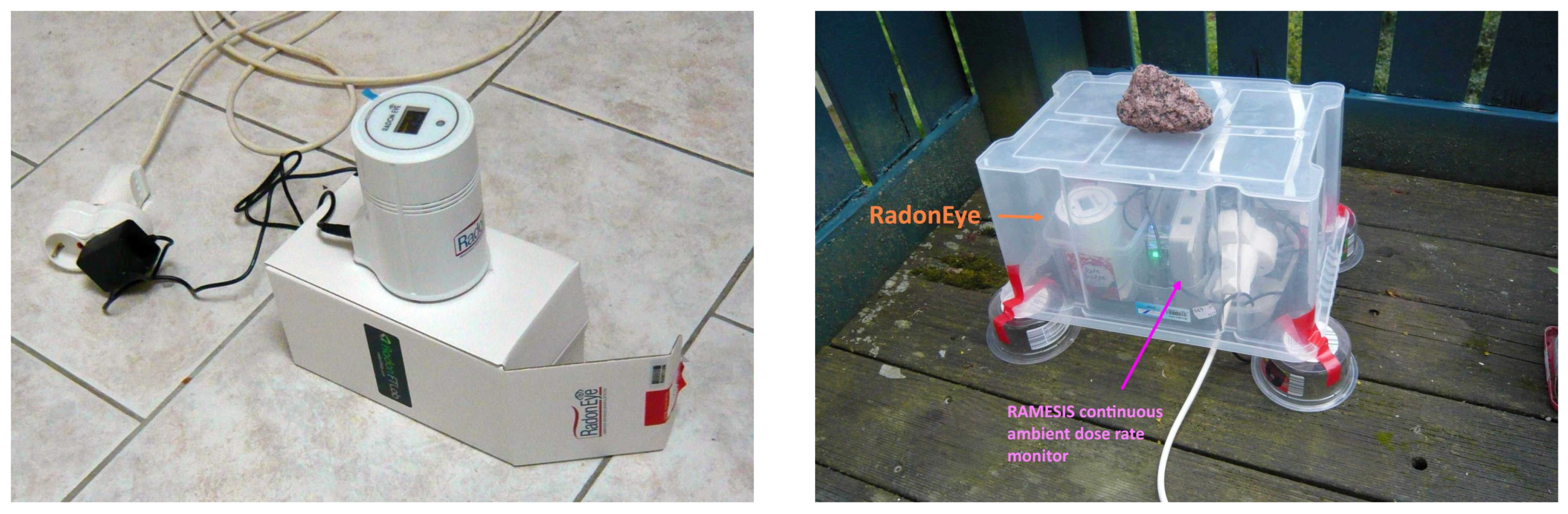
Figure 2.
Critical limits in dependence of instrument background;
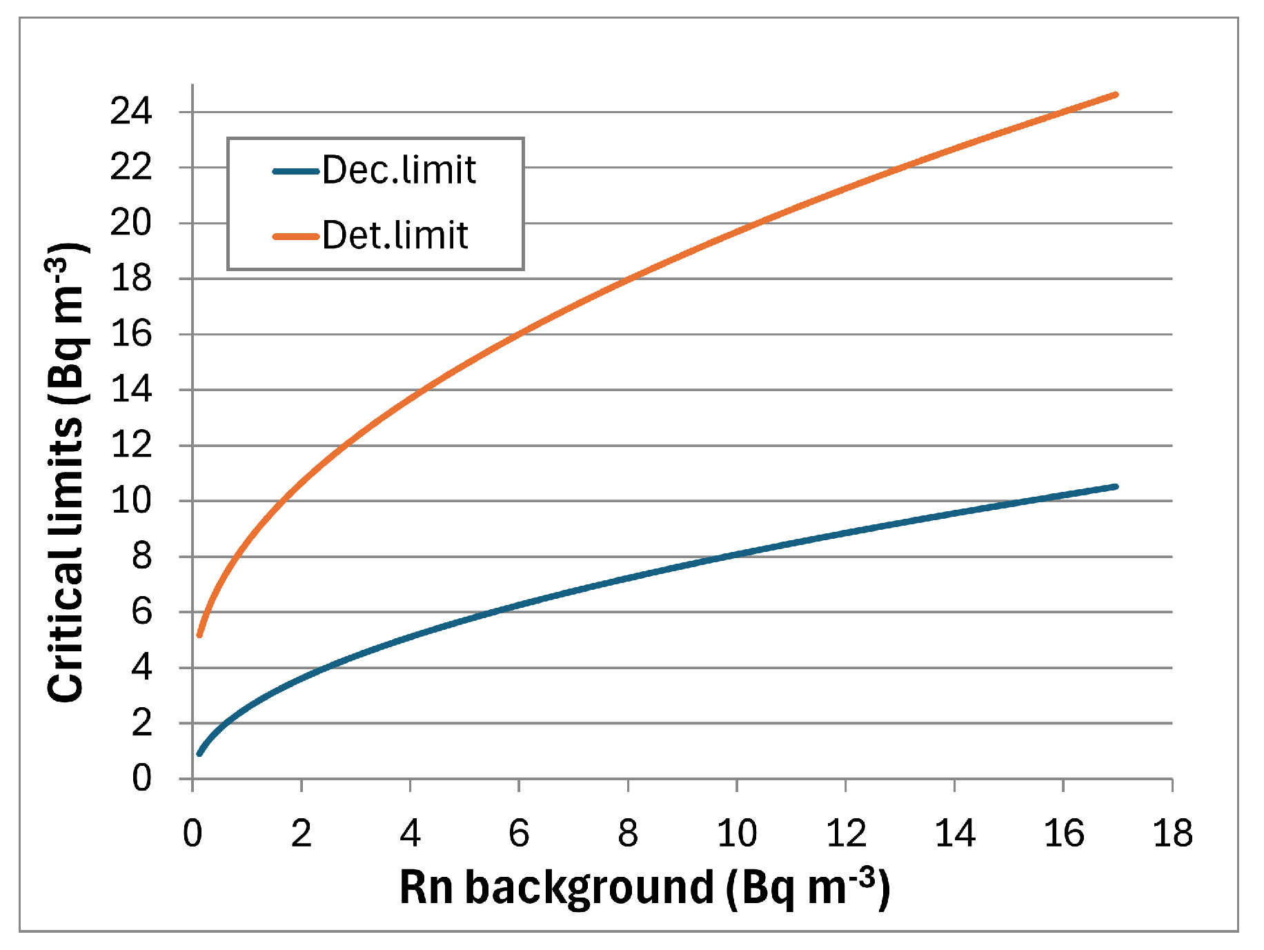
Figure 3.
(a) Relative uncertainty (1 ) of measurement results of the RadonEye; (b) Frequentist Poisson confidence limits of the Poisson mean for =0.05, midpoint of the confidence interval and Bayesian estimate of the mean. 1 count per hour (the reporting period) corresponds to about 1.2 Bq m.
Figure 3.
(a) Relative uncertainty (1 ) of measurement results of the RadonEye; (b) Frequentist Poisson confidence limits of the Poisson mean for =0.05, midpoint of the confidence interval and Bayesian estimate of the mean. 1 count per hour (the reporting period) corresponds to about 1.2 Bq m.
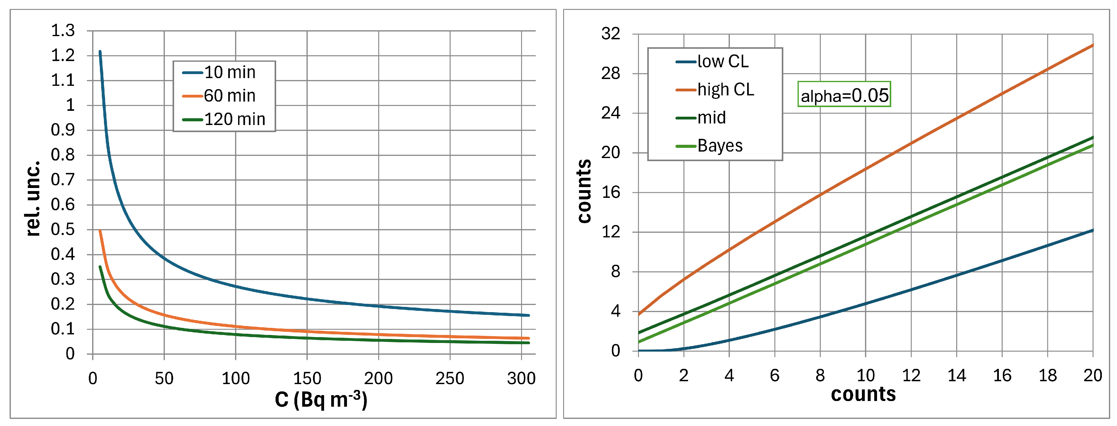
Figure 4.
Main graph: Expected and most probable true Rn concentration in dependence of the reported concentration. lower-right inset: Relative deviation of expected from reported concentration; upper-left inset: Relative deviation of corresponding expected from observed count number.
Figure 4.
Main graph: Expected and most probable true Rn concentration in dependence of the reported concentration. lower-right inset: Relative deviation of expected from reported concentration; upper-left inset: Relative deviation of corresponding expected from observed count number.
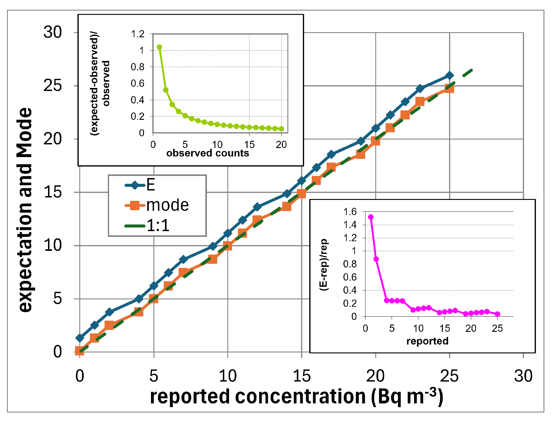
Figure 5.
Relation between reported concentration, Bq m rounded to integers, and count number k, for two values of cal given in the legend.
Figure 5.
Relation between reported concentration, Bq m rounded to integers, and count number k, for two values of cal given in the legend.
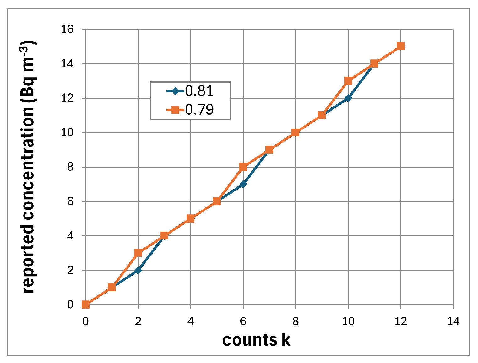
Figure 6.
: Radon concentration time series from Vienna and Berlin. Sampling periods 1 h.
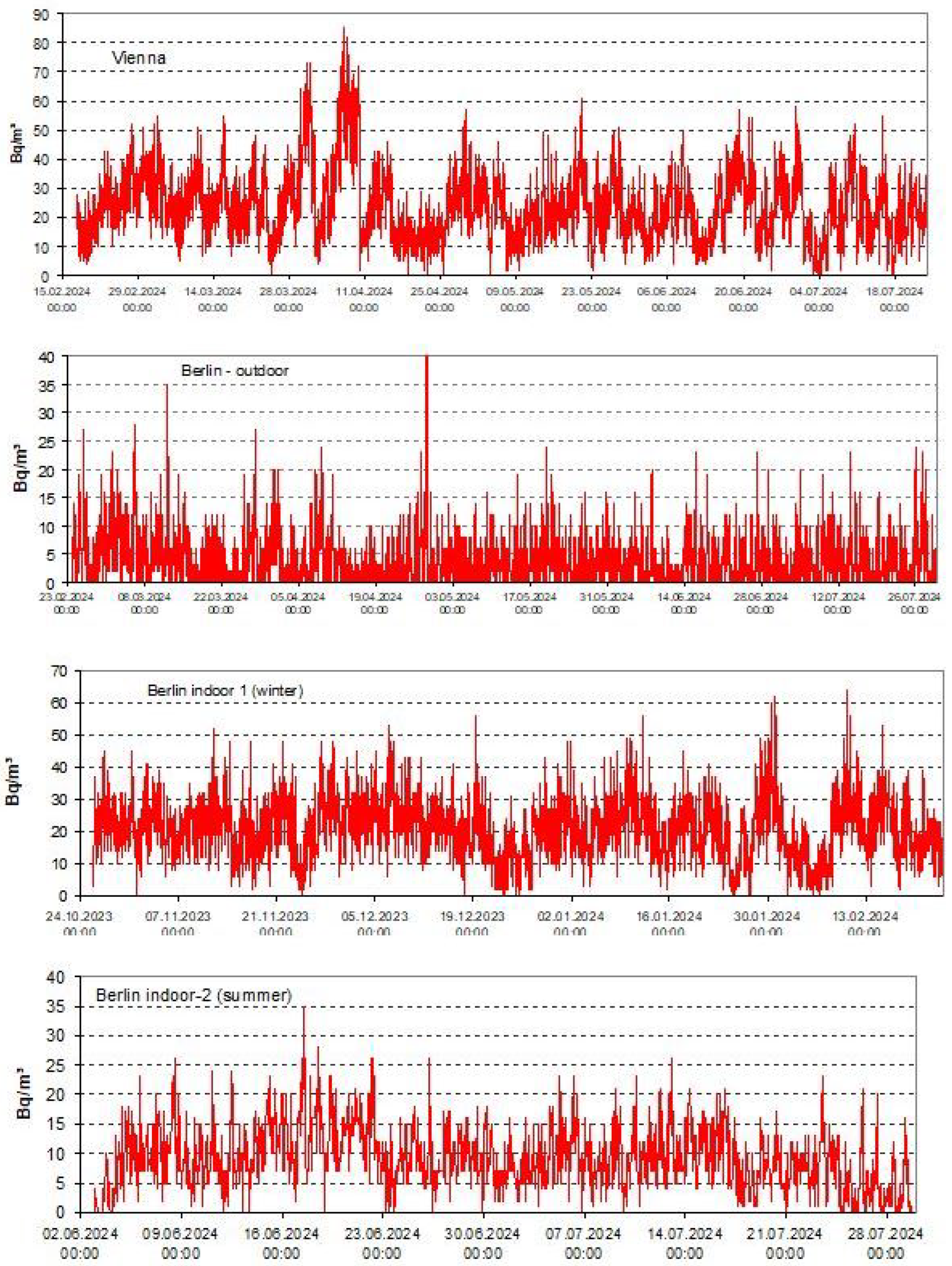
Figure 7.
Short-term variability of outdoor Rn concentration, Berlin, mid-August 2024
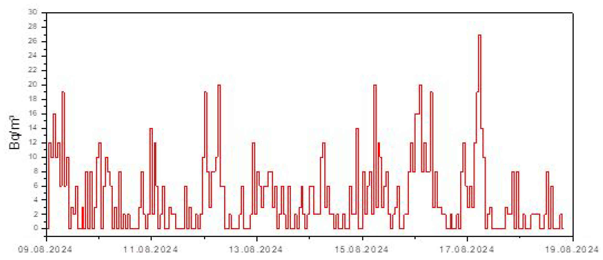
Figure 8.
Upper graph: Fourier plots of the three time series. Inset: log-log periodogram of the Viennese series; black lines drawn as guide to the eye. Lower graph: Autocorrelation plots of the four time series (raw data). 1/e: criterion to determine the correlation length.
Figure 8.
Upper graph: Fourier plots of the three time series. Inset: log-log periodogram of the Viennese series; black lines drawn as guide to the eye. Lower graph: Autocorrelation plots of the four time series (raw data). 1/e: criterion to determine the correlation length.
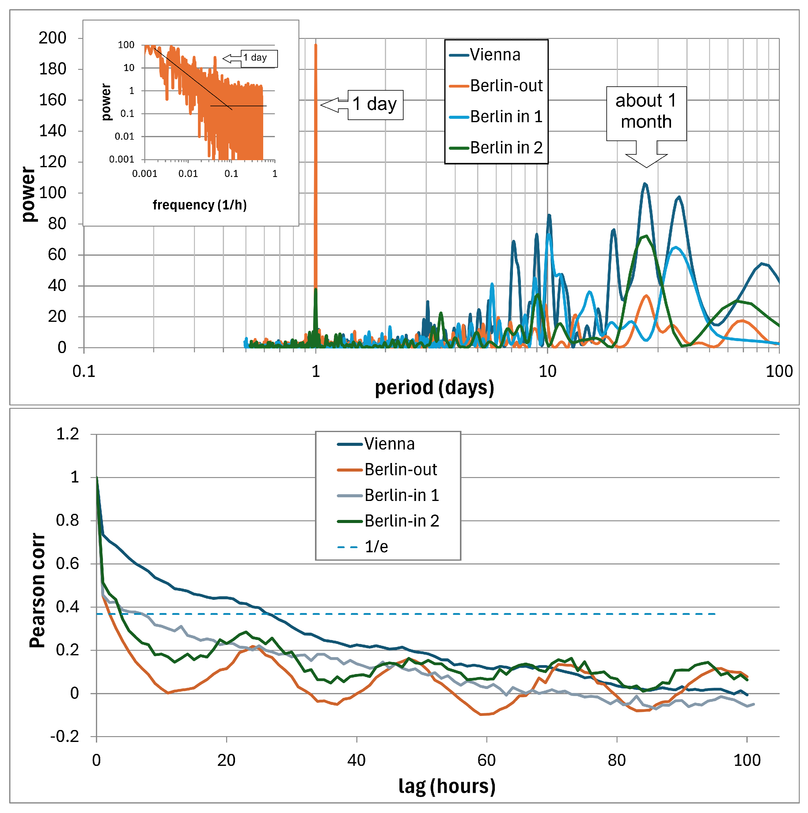
Figure 9.
Cross-correlation plot between outdoor and indoor Rn concentration, Berlin.
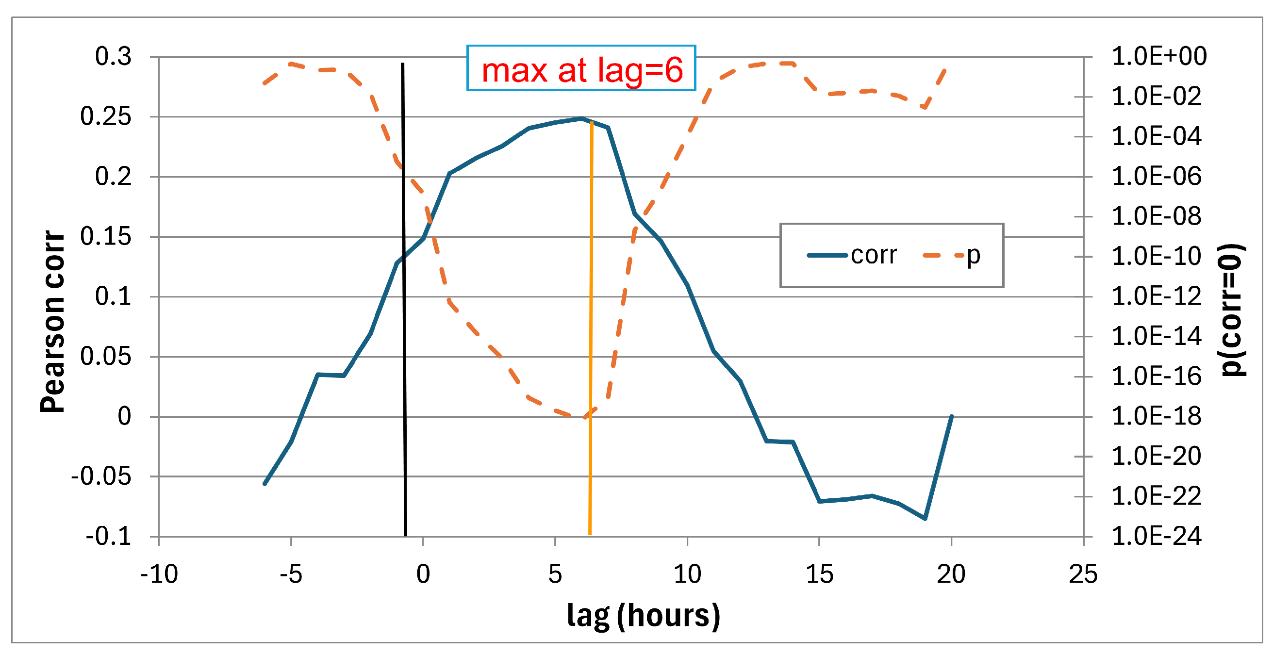
Figure 10.
Ratio outdoor / indoor concentrations, Berlin.
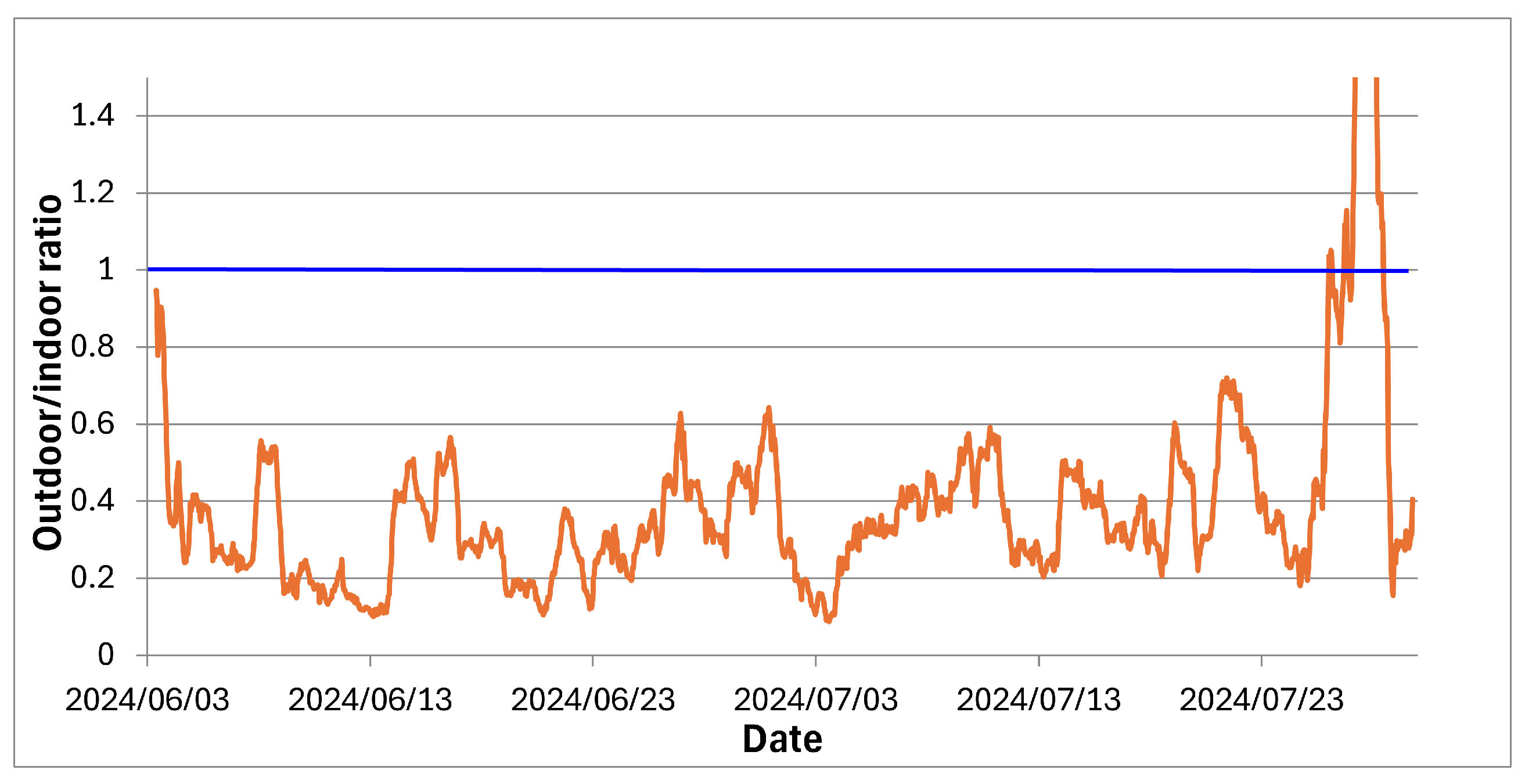
Figure 11.
Mean and quantiles of outdoor Rn concentration, Berlin, per hour of the day, for the entire measurement period.
Figure 11.
Mean and quantiles of outdoor Rn concentration, Berlin, per hour of the day, for the entire measurement period.
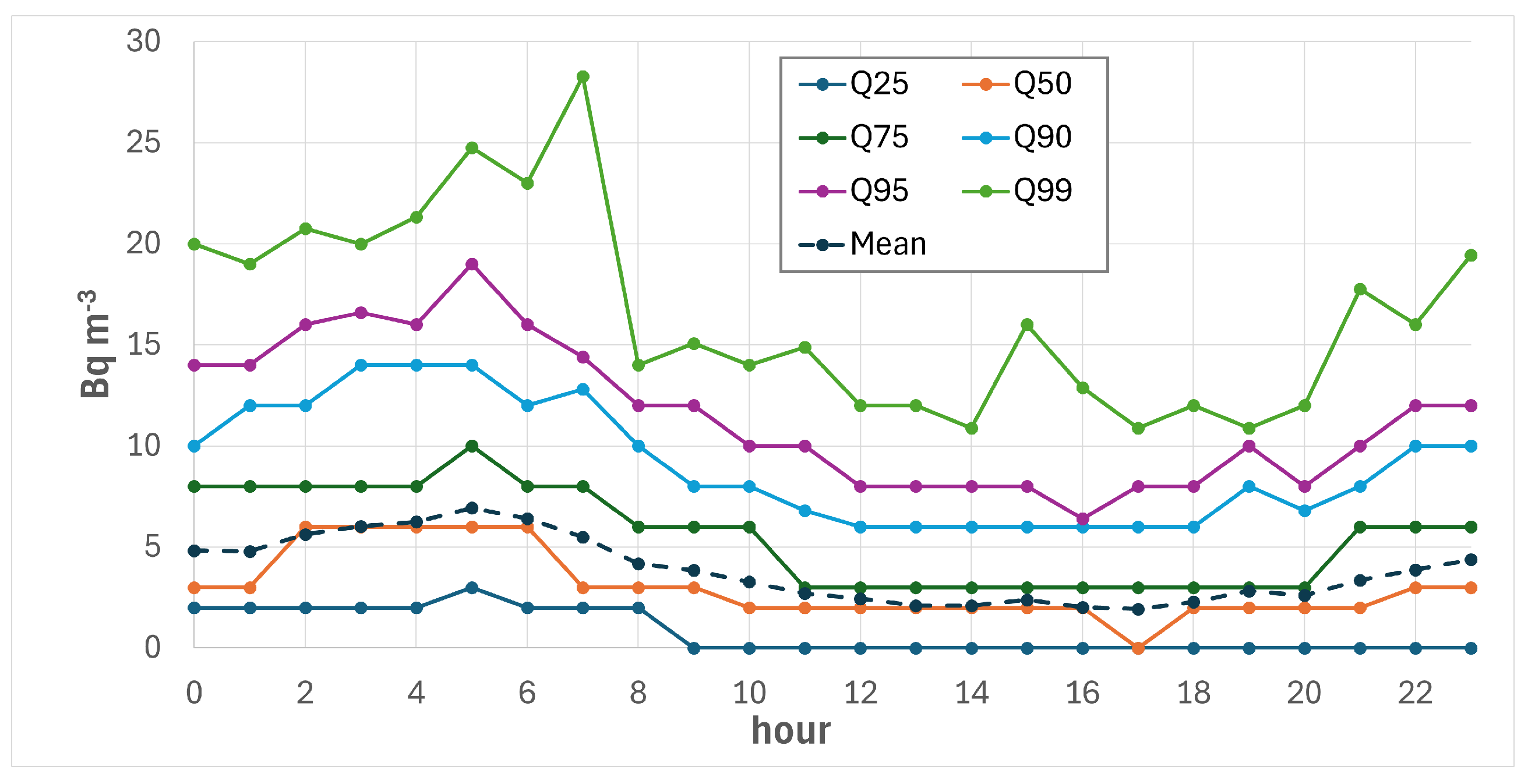
Figure 12.
Left: Mean outdoor Rn concentration, Berlin, per hour and month. Right: hour of the day when the highest Rn concentration occurs (aggregation period: 4 weeks sliding window)
Figure 12.
Left: Mean outdoor Rn concentration, Berlin, per hour and month. Right: hour of the day when the highest Rn concentration occurs (aggregation period: 4 weeks sliding window)
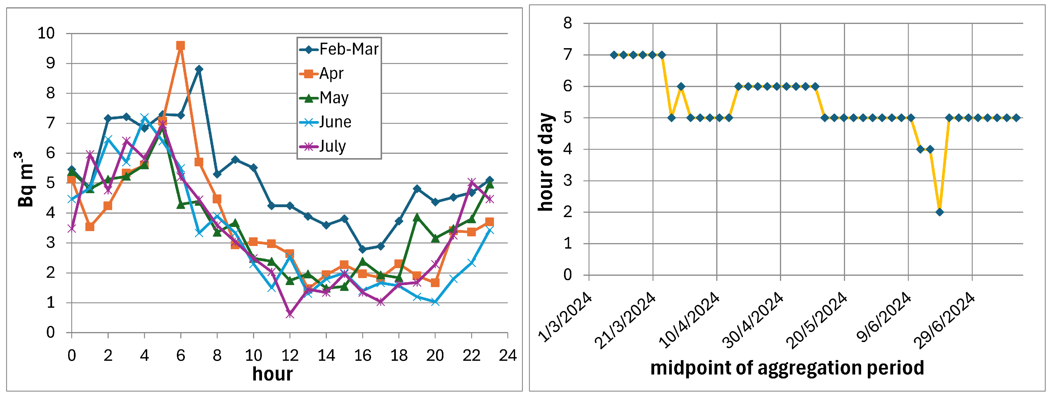
Figure 13.
Maxima of Rn concentration, Berlin outdoors.
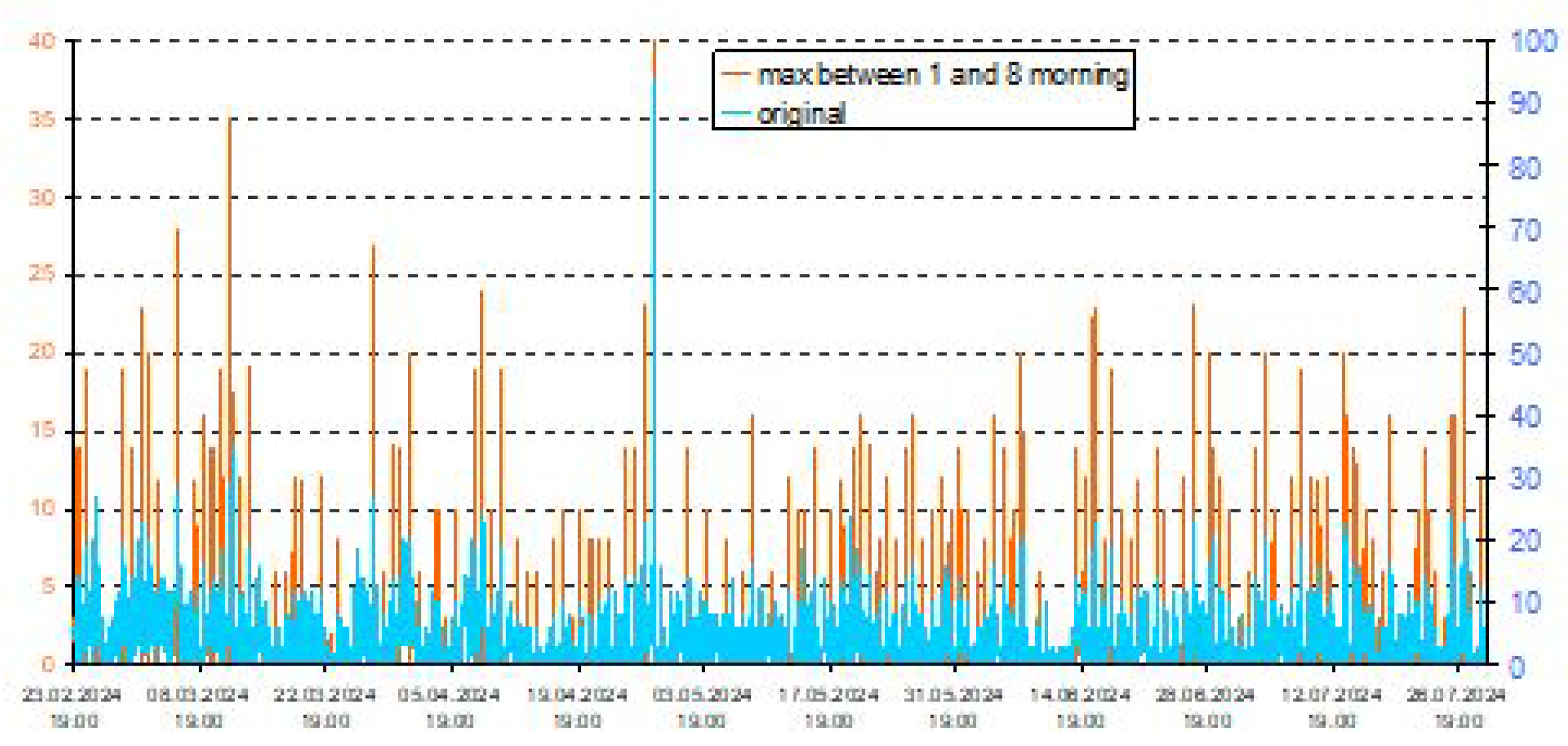
Figure 14.
ARMA(5,1) modelled Rn time series, Vienna.
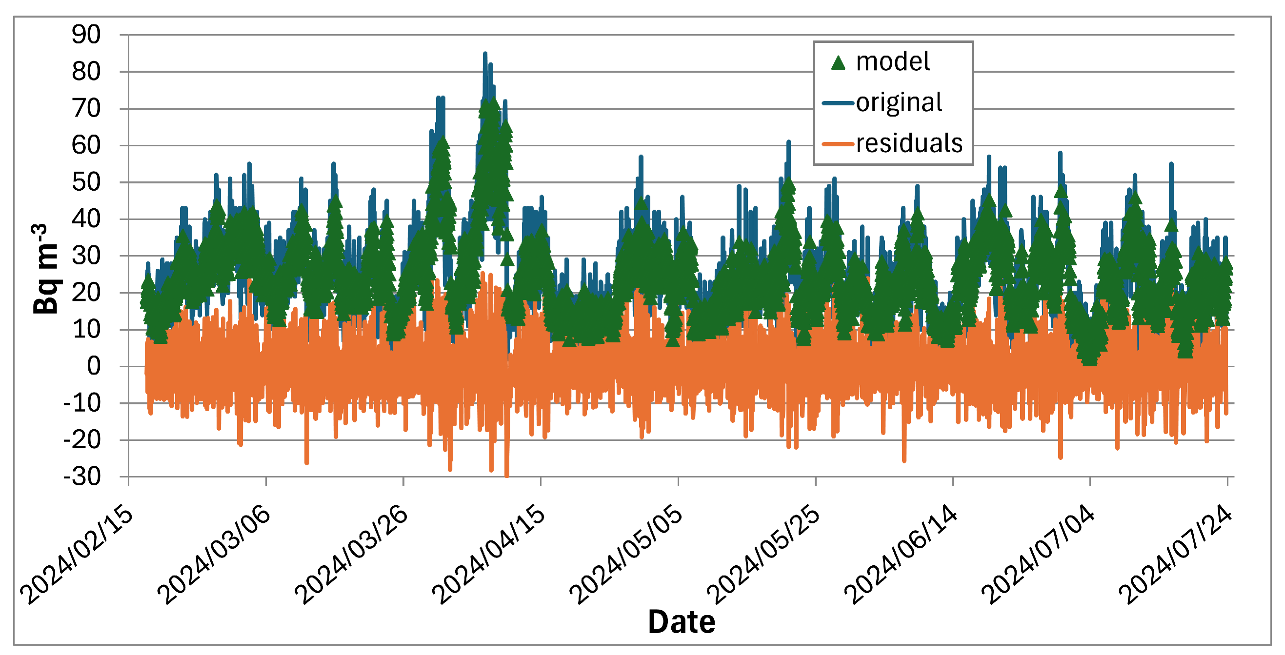
Figure 15.
ACF and PACF of the raw Viennese series. The PACF suggest 4 to 5 AR components.
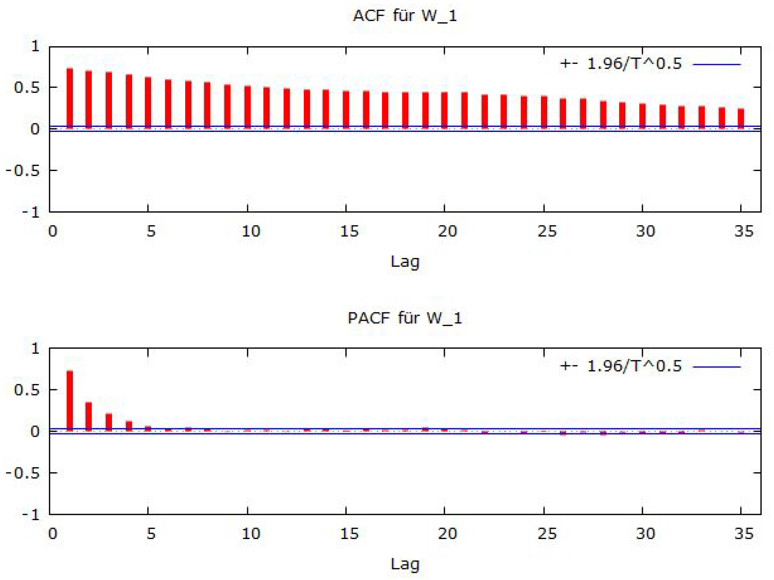
Figure 16.
Example for the determination of the Hurst exponent H (exponent of the power model) with in-house developed software. Orange graph: from the ensemble of 10 random tracks; blue: from the ensemble mean.
Figure 16.
Example for the determination of the Hurst exponent H (exponent of the power model) with in-house developed software. Orange graph: from the ensemble of 10 random tracks; blue: from the ensemble mean.
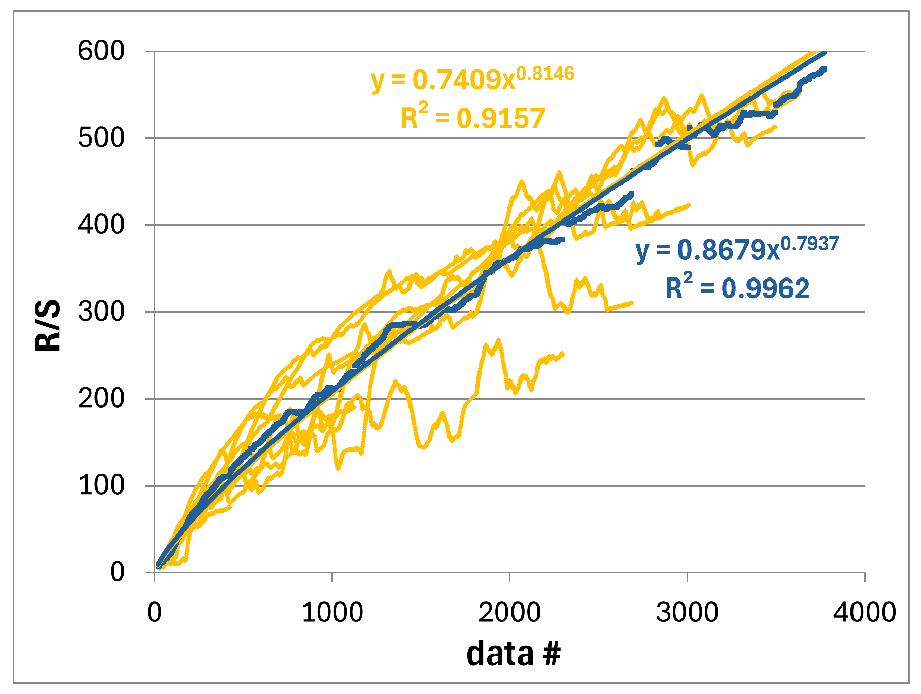
Figure 17.
spectra of the Rn time series. For the Berlin outdoor series uncertainties are added which represent 1 standard error of the slope estimated by linear regression. Only points with regression Pearson correlation >0.9 were used.
Figure 17.
spectra of the Rn time series. For the Berlin outdoor series uncertainties are added which represent 1 standard error of the slope estimated by linear regression. Only points with regression Pearson correlation >0.9 were used.
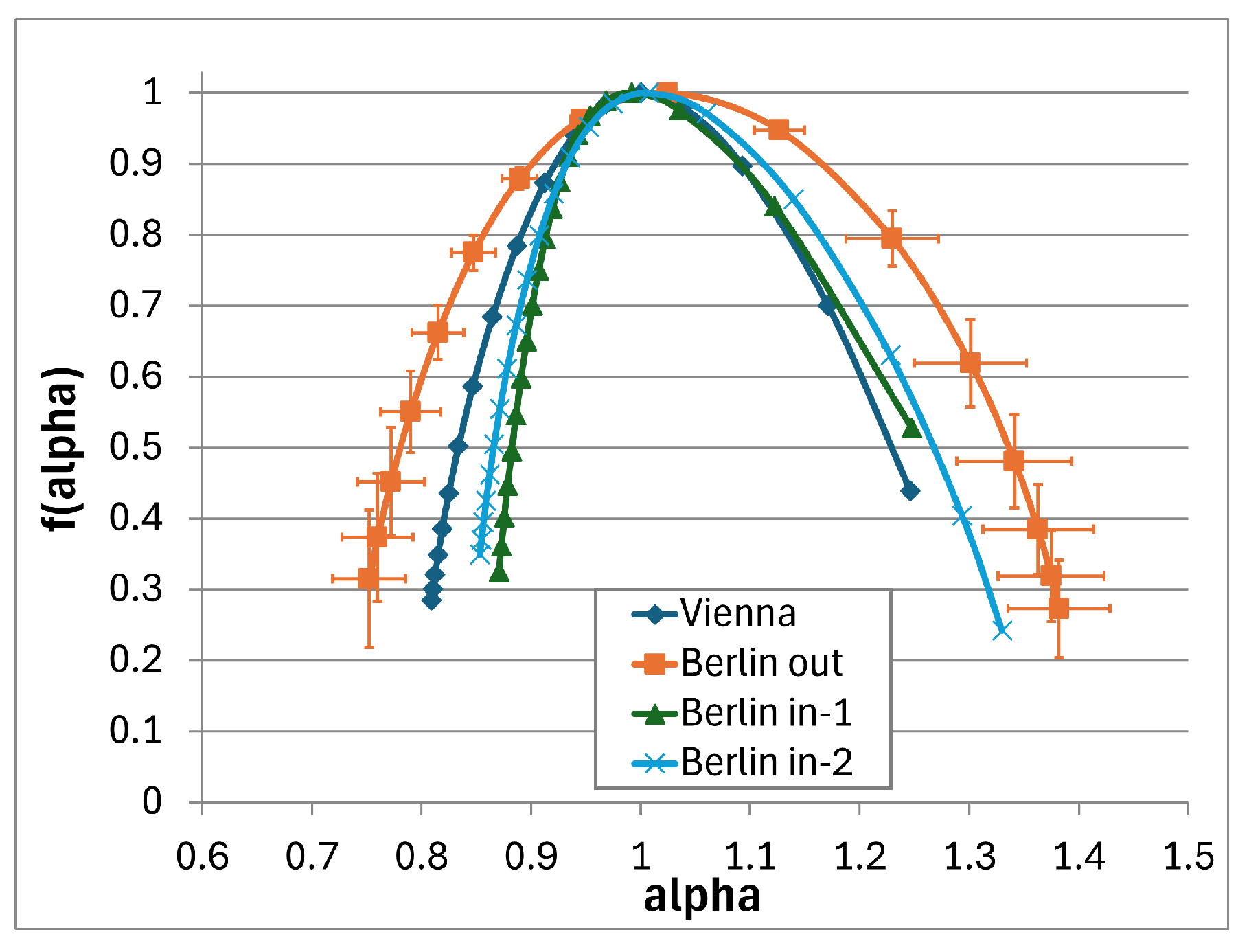
Figure 18.
Determination of the box dimension of the time series.
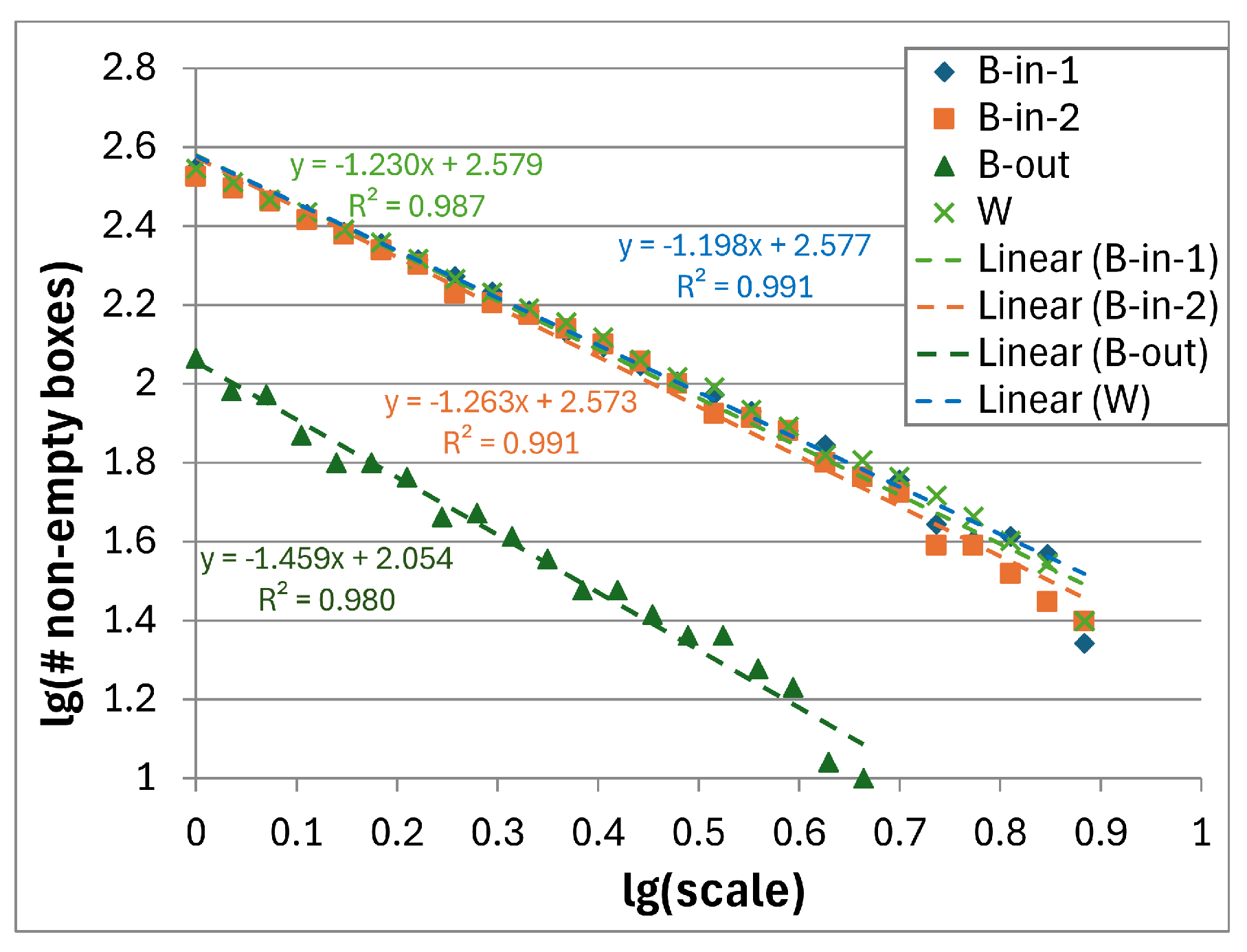
Figure 19.
Graph to determine the Garger exponent through linear regression.
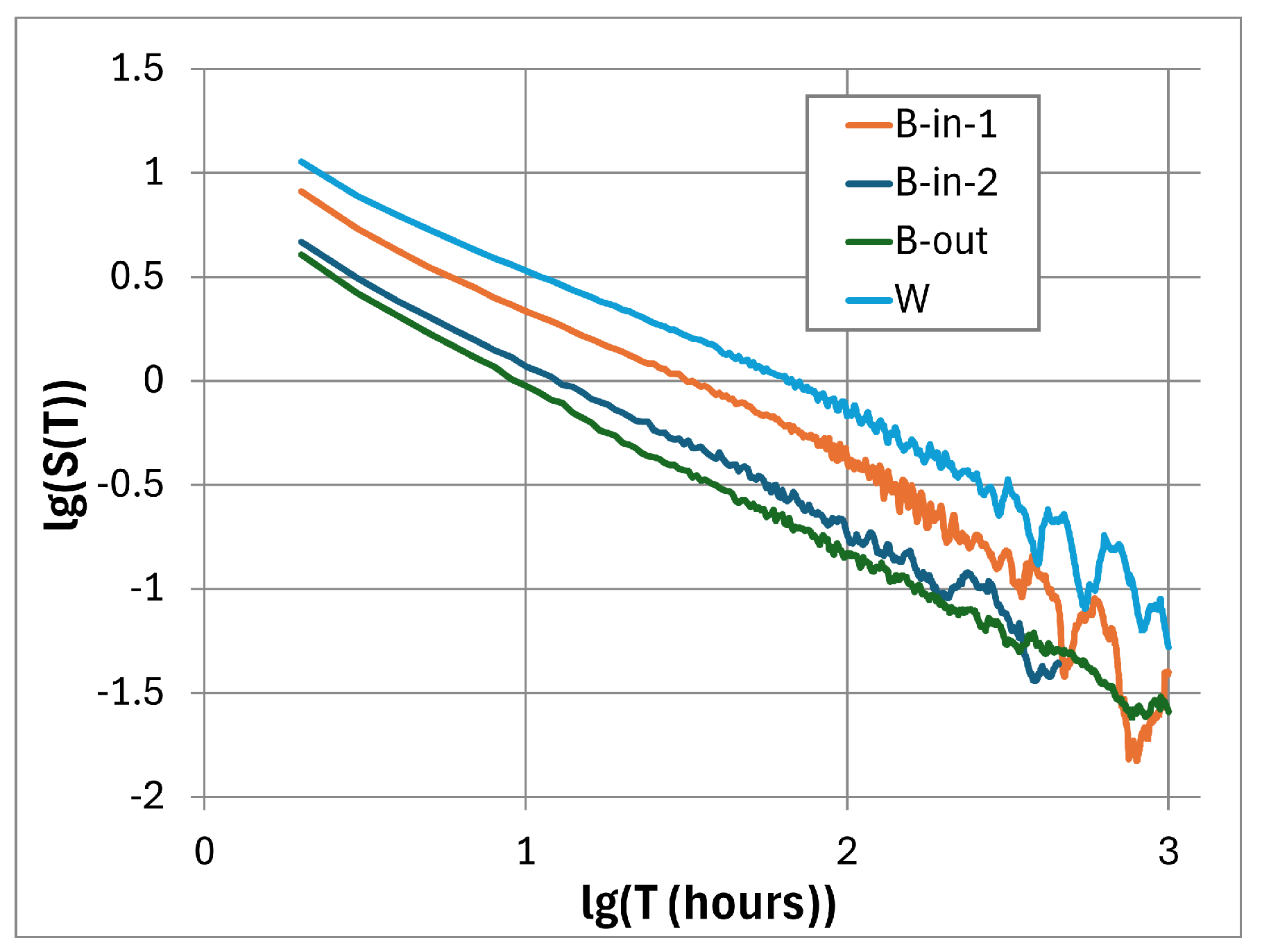
Figure 20.
Outputs of CDA 1.1 software to determine the embedding dimension E.
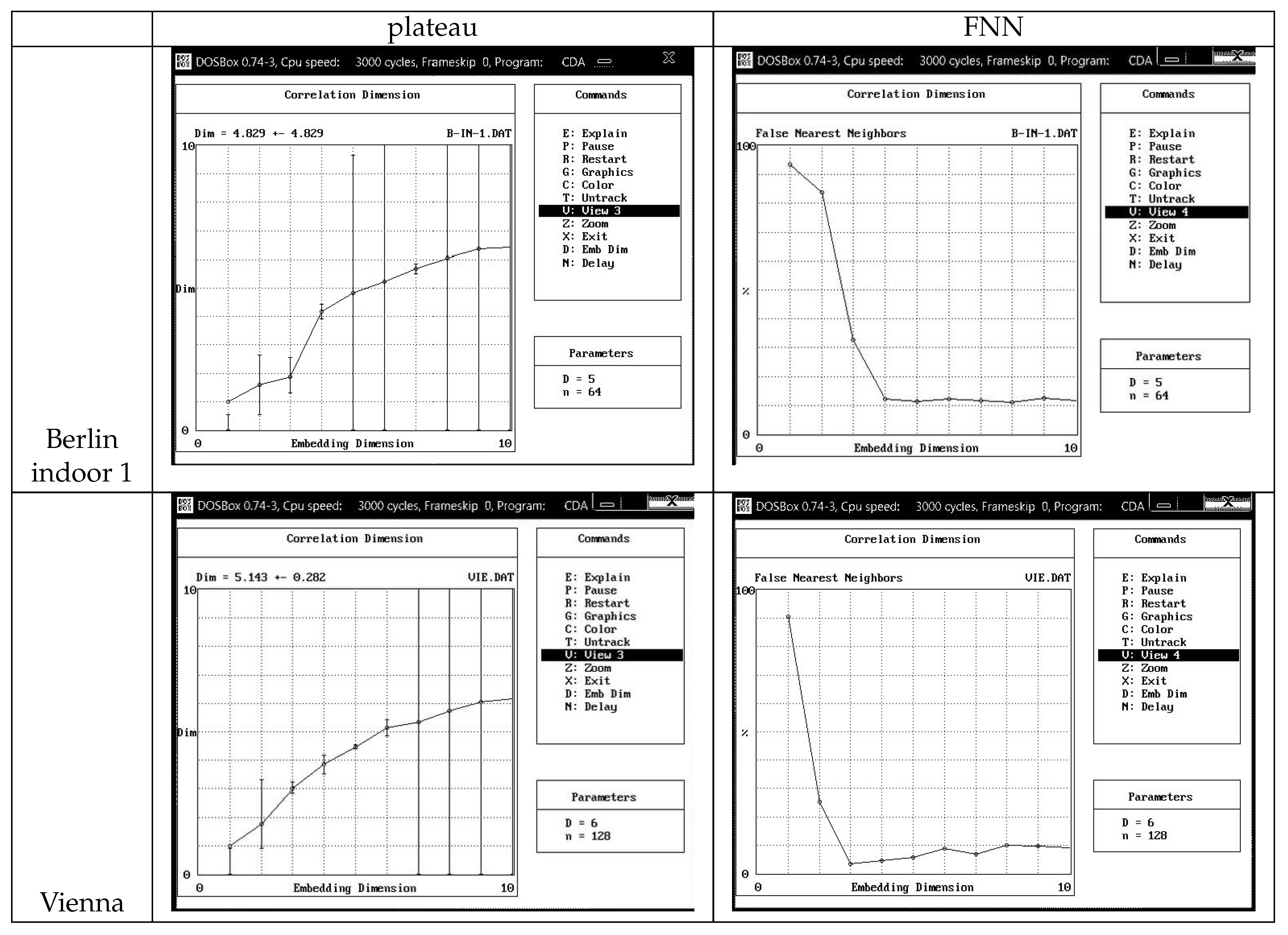
| plateau | FNN | |
| Berlin indoor 1 |
||
| Vienna |
| Berlin |
| indoor 1 |

Table 1.
Given true concentration C(true), the probability for a reported concentration C(rep), third column, is given in the table.
Table 1.
Given true concentration C(true), the probability for a reported concentration C(rep), third column, is given in the table.
| C(true)= → | 0.5 | 1 | 1.5 | 2 | 2.5 | 3 | 3.5 | 4 | 4.5 | ||
|---|---|---|---|---|---|---|---|---|---|---|---|
| = → | 0.405 | 0.81 | 1.215 | 1.62 | 2.025 | 2.43 | 2.835 | 3.24 | 3.645 | ||
| k= ↓ | C(reg)=↓ | C(rep)=↓ | p(k)= | ||||||||
| 0 | 0 | 0 | 0.667 | 0.445 | 0.297 | 0.198 | 0.132 | 0.088 | 0.059 | 0.039 | 0.026 |
| 1 | 1.234 | 1 | 0.27 | 0.36 | 0.361 | 0.321 | 0.267 | 0.214 | 0.166 | 0.127 | 0.095 |
| 2 | 2.469 | 2 | 0.055 | 0.146 | 0.219 | 0.26 | 0.271 | 0.26 | 0.236 | 0.206 | 0.174 |
| 3 | 3.704 | 4 | 0.007 | 0.039 | 0.089 | 0.14 | 0.183 | 0.211 | 0.223 | 0.222 | 0.211 |
| 4 | 4.938 | 5 | 7E-04 | 0.008 | 0.027 | 0.057 | 0.092 | 0.128 | 0.158 | 0.18 | 0.192 |
| 5 | 6.172 | 6 | 6E-05 | 0.001 | 0.007 | 0.018 | 0.037 | 0.062 | 0.09 | 0.117 | 0.14 |
| 6 | 7.407 | 7 | 4E-06 | 2E-04 | 0.001 | 0.005 | 0.013 | 0.025 | 0.042 | 0.063 | 0.085 |
| 7 | 8.642 | 9 | 2E-07 | 2E-05 | 2E-04 | 0.001 | 0.004 | 0.009 | 0.017 | 0.029 | 0.044 |
| 8 | 9.877 | 10 | 1E-08 | 2E-06 | 3E-05 | 2E-04 | 9E-04 | 0.003 | 0.006 | 0.012 | 0.02 |
| 9 | 11.11 | 11 | 5E-10 | 2E-07 | 5E-06 | 4E-05 | 2E-04 | 7E-04 | 0.002 | 0.004 | 0.008 |
| 10 | 12.35 | 12 | 2E-11 | 1E-08 | 6E-07 | 7E-06 | 4E-05 | 2E-04 | 5E-04 | 0.001 | 0.003 |
| 11 | 13.58 | 14 | 8E-13 | 1E-09 | 6E-08 | 1E-06 | 8E-06 | 4E-05 | 1E-04 | 4E-04 | 1E-03 |
| 12 | 14.82 | 15 | 3E-14 | 7E-11 | 6E-09 | 1E-07 | 1E-06 | 8E-06 | 3E-05 | 1E-04 | 3E-04 |
| 13 | 16.05 | 16 | 0 | 5E-12 | 6E-10 | 2E-08 | 2E-07 | 1E-06 | 7E-06 | 3E-05 | 8E-05 |
| 14 | 17.28 | 17 | 0 | 3E-13 | 5E-11 | 2E-09 | 3E-08 | 3E-07 | 1E-06 | 6E-06 | 2E-05 |
| 15 | 18.52 | 19 | 0 | 0 | 4E-12 | 2E-10 | 4E-09 | 4E-08 | 3E-07 | 1E-06 | 5E-06 |
Table 2.
Missing nominal concentration values of three RadonEye devices.
| device id. | missing concentration values (Bq m) |
|---|---|
| GJ17RE000076 | 3, 6, 9, 12, 15, 18, 21, 24,... |
| RE22207111958 | 1, 3, 4, 5, 9, 11, 13, 15, 17, 18,... |
| HG04RE000641 | 3, 6 ,8, 11, 13,... |
Table 3.
Exploratory statistics of the radon concentration time series. n - number of data = total measurement time (hours), AM - arithmetic mean, SD - standard deviation, CV - coefficient of variation, Med - median.
Table 3.
Exploratory statistics of the radon concentration time series. n - number of data = total measurement time (hours), AM - arithmetic mean, SD - standard deviation, CV - coefficient of variation, Med - median.
| Vienna | Berlin-outdoor | Berlin-indoor 1 (winter) | Berlin-indoor 2 (summer) | |
|---|---|---|---|---|
| n | 3773 | 3768 | 2904 | 1365 |
| AM (Bq m) | 24 | 3.9 | 20.9 | 9.2 |
| SD (Bq m) | 12 | 4.7 | 9.5 | 5.3 |
| CV (%) | 51 | 123 | 46 | 58 |
| Min (Bq m) | 0 | 0 | 0 | 0 |
| Max (Bq m) | 85 | 60 (94) | 64 | 35 |
| Med (Bq m) | 22 | 2 | 20 | 9 |
| device # | GJ17RE000076 | RE22207111958 | RE22207111958 | HG04RE000641 |
the peak Bq m seems to be an outlier, perhaps some electronic disturbance
Table 4.
Periodicities and autocorrelation.
| Vienna | Berlin outdoor | Berlin indoor 1 |
Berlin indoor 2 |
|
|---|---|---|---|---|
| Periods (d) | 1; 3.1; 26.2 | 1; 9.7; 13.2; 26.7 | 1; 5.8; 8.1; 10; 35.8 | 1; 3.5; 9.1; 26.7 |
| log-log slope | ≈ 0.9 | ≈ 0.4 | ≈ 0.7 | ≈ 0.6 |
| Autocorr ≥e-1=0.37 (h) | 26 | 2 | 6 | 4 |
| Autocorr ≥ p=0.05 (h) | 77 | 8 | 55 | 36 |
Table 5.
AR and AM coefficients (see text)
| coefficients | Berlin-out | Berlin-in 1 | Berlin-in 2 | Vienna |
|---|---|---|---|---|
| AR coefficients | ||||
| 1 | -1.32 | -0.997 | -1.28 | -1.29 |
| 2 | 0.165 | 0.119 | 0.128 | |
| 3 | 0.079 | 0.023 | 0.036 | |
| 4 | 0.035 | 0.137 | 0.058 | |
| 5 | 0.035 | 0.068 | ||
| AM coefficients | ||||
| 1 | -0.995 | -0.807 | -0.973 | -0.926 |
| AIC opt | 2.136e4 | 2.021e4 | 7874 | 2.586e4 |
| mean rel.res | 3.71 | 1.35 | 1.74 | 1.25 |
Table 6.
Hurst coefficients estimated by different software (for the graph dimension DB see Section 5.3.3)
Table 6.
Hurst coefficients estimated by different software (for the graph dimension DB see Section 5.3.3)
| statistic | Berlin out | Berlin in-1 | Berlin in-2 | Vienna |
|---|---|---|---|---|
| Custom | 0.64 | 0.76 | 0.84 | 0.82 |
| H=2-DB | 0.54 | 0.77 | 0.74 | 0.80 |
| Gretl | 0.73 | 0.81 | 0.86 | 0.87 |
| R, "corr. R/S" | 0.74 | 0.81 | 0.87 | 0.87 |
| R, "corr. empir" | 0.66 | 0.78 | 0.70 | 0.75 |
Table 7.
Various fractal statistics of the Rn time series. For the definitions of the statistics see the text. For details of E and L, see Section 5.3.3. In this table, E are summarized according to the detailed results. "low" Lyapunov means < 0.01, which is difficult to estimate with our means.
Table 7.
Various fractal statistics of the Rn time series. For the definitions of the statistics see the text. For details of E and L, see Section 5.3.3. In this table, E are summarized according to the detailed results. "low" Lyapunov means < 0.01, which is difficult to estimate with our means.
| statistic | Berlin out | Berlin in-1 | Berlin in-2 | Vienna |
|---|---|---|---|---|
| Garger g | 0.815 ± 0.005 | 0.698 ± 0.004 | 0.780 ± 0.005 | 0.658 ± 0.003 |
| Graph dim | 1.457 ± 0.049 | 1.230 ± 0.029 | 1.263 ± 0.026 | 1.198 ± 0.023 |
| Lyapunov L | low | low | low | low |
| Embed dim E | ∼6 | 4 - 6 | 5 | 3 - 5 |
Table 8.
Minimum embedding dimension E estimated with CDA software. - delay time, FNN - false nearest neighbour statistic, plateau - E for which the correlation dimension of the embedded time series approximately reaches a plateau. n - no conclusive result.
Table 8.
Minimum embedding dimension E estimated with CDA software. - delay time, FNN - false nearest neighbour statistic, plateau - E for which the correlation dimension of the embedded time series approximately reaches a plateau. n - no conclusive result.
| (h) | FNN | plateau | |
|---|---|---|---|
| Vienna | 128 | ∼ 3 | 6 ? |
| Berlin outdoor | 8 | n | 6 |
| Berlin indoor 1 | 64 | 5 | 5 ? |
| Berlin indoor 2 | 32 | 5 | 5 |
Table 9.
Embedding dimension E and maximal Lyapunov exponent estimated with R software. n.p. - no plausible result, n - no interpretable result
Table 9.
Embedding dimension E and maximal Lyapunov exponent estimated with R software. n.p. - no plausible result, n - no interpretable result
| (h) | E (tseriesChaos) |
E (nonlinearTseries) |
L (tseriesChaos) |
L (nonlinearTseries) |
|
|---|---|---|---|---|---|
| Vienna | 80 18 |
4 4 |
n.p. n.p. |
0.001 0.004 |
0.21 - 0.41 0.28 |
| Berlin outdoor | 8 30 |
6 7 |
n n.p. |
0.003 n |
0.055 - 0.35 0.28 - 0.52 |
| Berlin indoor 1 | 50 18 |
4 - 6 4 |
n.p. n.p. |
n 0.002 - 0.003 |
0.20 - 0.32 0.16 |
| Berlin indoor 2 | 36 18 |
5 - 6 5 |
n.p. n.p. |
0.002 0.001 |
0.19 0.37 |
Disclaimer/Publisher’s Note: The statements, opinions and data contained in all publications are solely those of the individual author(s) and contributor(s) and not of MDPI and/or the editor(s). MDPI and/or the editor(s) disclaim responsibility for any injury to people or property resulting from any ideas, methods, instructions or products referred to in the content. |
© 2024 by the authors. Licensee MDPI, Basel, Switzerland. This article is an open access article distributed under the terms and conditions of the Creative Commons Attribution (CC BY) license (http://creativecommons.org/licenses/by/4.0/).
Copyright: This open access article is published under a Creative Commons CC BY 4.0 license, which permit the free download, distribution, and reuse, provided that the author and preprint are cited in any reuse.


