
Submitted:
25 March 2025
Posted:
26 March 2025
You are already at the latest version
Abstract
Vortex-induced vibration (VIV) is a common fluid-structure interaction phenomenon in practical engineering with significant research value. Traditional methods to solve VIV issues include experimental studies and numerical simulations. However, experimental studies are costly and time-consuming, while numerical simulations are constrained by low Reynolds numbers and simplified models. Using large amount of training data, deep learning (DL) can successfully capture VIV patterns and generate accurate predictions. Physics Informed Neural Networks (PINNs), a subfield of DL, introduces physics equations into the loss function to reduce the need for large data. However, PINN loss functions often include multiple loss terms, which may interact with each other, causing imbalanced training speeds of the model and a potentially inferior overall performance. To address this issue, the study proposes an adaptive-weight physics-informed neural network (AW-PINN) algorithm built upon the gradient normalization method (GardNorm) from multi-task learning. AW-PINN regulates the weights of each loss term by computing the gradients norms on the network weights, ensuring the norms of the loss terms match predefined target values. This allows for the balance in the training speed for each loss term and improves both prediction precision and robustness of network model alike. In this study, a VIV dataset of a cylindrical body with different degrees of freedom was used to compare the performance of PINN and three PINN optimization algorithms. The findings suggest that, compared to standard PINN, AW-PINN lowers the mean squared error (MSE) on the test set by 50%, significantly improving prediction accuracy. AW-PINN also demonstrates better stability across different datasets compared to other optimization algorithms, which reveals AW-PINN is a robust and reliable algorithm for solving VIV problems.
Keywords:
Vortex-induced vibration
; Deep learning
; Physics-informed neural network
; Gradient normalization
; Adaptive weights
1. Introduction
Vortex-induced vibration (VIV) is a common phenomenon in various engineering structures, including the cables of long-span bridges [1,2,3], wind turbine towers [4,5], and risers of offshore platforms [6,7]. When a bluff body is placed in a flowing fluid, alternating vortex shedding occurs on both sides of the boundary layer. This vortex shedding causes periodic variations in the lift and drag forces acting on the body, which, in turn, induces vibrations in the structure. The interaction between the fluid and the structure is referred to as VIV [8]. When the vortex-shedding frequency approaches the structure’s natural frequency, the vibration amplitude may increase dramatically, potentially causing fatigue failure and posing a significant threat to the structural integrity, thereby reducing the structure's service life [9].
The investigation of VIV can be approached through various methods, including experimental research [10,11], semi-empirical models [12,13], and numerical simulation [14,15]. Experimental studies enable the observation of phenomena through physical models and the collection of data; however, this approach is costly and time-consuming due to the need for model fabrication. Based on experimental data and theoretical research, several semi-empirical models were proposed to predict the VIV characteristics [16]. With advancements in computational technology, numerical simulations have become a crucial tool for VIV research, including methods like Direct Numerical Simulation (DNS) [17,18], Large Eddy Simulation [19,20], as well as Reynolds-Averaged Navier-Stokes (RANS) models [21,22,23]. Numerical simulations offer a cost-effective means to address most VIV problems and can precisely predict both the flow field and structural motion. Nevertheless, numerical simulations require significant computational resources, making efficient predictions a challenge [24], when dealing with high Reynolds number turbulent flows and complex geometries. Therefore, accurately and efficiently solving VIV problems remains a highly demanding task.
Deep learning (DL), as one of the core research areas in AI, has been widely applied across various industries [25]. Compared to traditional machine learning, deep learning offers superior data processing capabilities. As the volume of data increases, the performance of deep learning models improves substantially, whereas traditional machine learning models tend to stabilize after a certain threshold, beyond which no further improvement occurs [26]. Deep learning is particularly effective at nonlinear fitting, allowing for the adjustment of network architectures through combinations of linear and nonlinear modules. In theory, it can map any function and solve complex problems in high-dimensional data [27]. In fluid dynamics, the application of deep learning has been growing, offering approximate solutions to a range of fluid dynamics problems [28]. Jin et al. [29] proposed a data-driven model integrating Convolutional Neural Networks (CNNs), using pressure data around a cylinder at different Reynolds numbers to predict the velocity field. Sekar et al. [30] built a data-driven method combining CNN and Multi-Layer Perceptron (MLP) for rapid flow field prediction. Kim et al. [31] utilized existing experimental data and deep neural networks to model VIVs of a cylinder, significantly reducing the need for experimental data. However, data-driven models require large amounts of training data to ensure predictive accuracy and are often not robust to noisy data [32]. Moreover, since these models do not incorporate physical prior knowledge, they lack interpretability and cannot provide guarantees of convergence [33].
To elevate the interpretability and robustness of data driven models and reduce their reliance on large datasets, Raissi et al. [33] introduced prior knowledge into the DL framework, proposing the Physics Informed Neural Network (PINN) to solve problems about partial differential equations. Through incorporating a physical information loss term into the loss function, PINN remarkably improves model performance in data-scarce scenarios. The implementation of this approach makes PINN capable of better capturing and simulating physical phenomena with fewer training data, improving the model’s predictive accuracy and reliability. Raissi et al. [34] incorporated the incompressible Navier-Stokes equations as physical constraints in PINN, utilizing spatiotemporal data of both velocity field and structural motion to reconstruct the fluid’s velocity and pressure fields, as well as to infer the lift and drag forces acting on the structures. Cheng et al. [35] integrated the RANS equations (with additional viscosity parameters) into the loss function to solve VIV and wake-induced vibrations (WIV) at various reduced velocities in turbulent flows. Tang et al. [36] proposed a Transfer Learning-Physics-Informed Neural Network to study VIVs of cylinders, leveraging transfer learning to reduce PINN's dependence on large datasets and thus lower training costs. Zhu et al. [37] applied PINN to learn VIV response data under varying stiffness conditions, enabling the prediction of VIV responses and the inference of structural stiffness. The PINN loss function combines data loss and various physical information losses with fixed weights. This approach enables PINN to simultaneously learn from data while embedding physical laws, improving both its predictive capability and generalization. However, during training, the gradients of the various loss terms in the PINN loss function can vary significantly during backpropagation, resulting in imbalanced training of each loss component. Wang et al. [38] identified this issue and explored potential solutions.
To elevate the performance and robustness of PINNs in solving complicated problems, many researchers have proposed different optimization algorithms. Xiang et al. [39] introduced an optimization algorithm for PINNs that automatically updates the weights in the training process. This method constructs a Gaussian probabilistic model, defines the loss function based on maximum likelihood estimation, and validates its effectiveness and robustness by solving classical partial differential problems. Chen et al. [40] delved into the impact of various weightings on PINN’s solution of the Richards-Richardson equation (RRE) and proposed a principled loss-function-based method that automatically adjusts the loss function weights without needing any hyperparameters, lowering PINN’s reliance on the initial weight settings. Tarbiyati et al. [41] trained and determined the initial weights of PINNs by solving partial differential equations with finite difference methods, and used the equation solutions to enhance the performance. In the application of PINNs to solve the Navier-Stokes equations, researchers have also proposed optimization algorithms. Li et al. [42] were inspired by the minmax algorithm and introduced a dynamic weighting strategy for solving both the forward and inverse issues of the Navier-Stokes equations. This strategy identifies the difficulty level of the training data and adjusts the weights of more difficult data to accelerate the training process, balancing the contributions of various data loss terms to the network. Hou et al. [43] proposed an adaptive loss balance PINN (LB-PINN) to reconstruct the propeller wake flow field. Through introducing adaptive weights, this method balances the different losses in the network, elevating the flow field reconstruction accuracy. Shi et al. [44] framed PINN as a multi task learning problem and introduced a method that automatically adjusts loss weights, balancing the training speed of different loss components and stabilizing the network’s training process.
In this study, we explore an Adaptive Weight Physics-Informed Neural Network (AW-PINN) incorporating the principles of multi-task learning. The neural network's training process is enhanced by AW-PINN's integration of the Gradient Normalization (GradNorm) algorithm to elevate the model's capacity to predict complicated phenomena in fluid dynamics. In AW-PINN, we use the gradient norm of the weight loss function with respect to the hidden layer weights of the network as the indicator for the training speed, and the average of the gradient norm of all weight loss terms as a common scale. AW-PINN adjusts the training speed of each loss term by the regulation of the weights of different loss components and adjusts their contribution to overall training. The network slows down its own training speed when the gradient norm of a certain loss term surpasses the target gradient norm, thereby reducing the weight of a particular loss term, so that all of the loss components can be trained at a comparable rate. We apply PINN, AW-PINN, and other optimization algorithms to different VIV datasets. Through comparisons of test errors across multiple datasets, we demonstrate that AW-PINN outperforms the other algorithms in performance and exhibits superior stability compared to other PINN optimization methods. The remainder of this research is organized as follows: Section 2 delivers a detailed description of the cylinder VIV problem, along with the principles behind PINN, GradNorm, and AW-PINN; Section 3 presents the training of various network models using datasets generated from numerical simulations, and verifies the stability of these models using additional datasets; Section 4 concludes the study.
2. Problem and Model
2.1. Research Problem
This study focuses on cylindrical structures, which are widely used in engineering, and investigates the application of the AW-PINN to solve the problem of VIV in cylinders. As illustrated in Figure 1, the study considers a two-dimensional elastically supported cylindrical structure and analyzes the two-dimensional VIV problem. The cylinder is simplified as a mass-spring-damping system that can move freely in both the streamwise direction (x-direction) and the transverse direction (y-direction).
In the rectangular coordinate system, the origin is set at the center of the cylinder, and a moving reference frame, which moves along with the cylinder, is established. The continuity equation for incompressible fluid as well as the momentum conservation equation (Navier-Stokes equations) [45] in the moving reference system are given by:

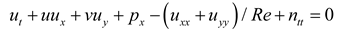
 where u and v represent the streamwise and transverse velocities of the flow field; p is the pressure in the flow field, and and are the streamwise as well as transverse displacements of the cylinder. Re is the dimensionless parameter, which characterizes the fluid flow behavior.
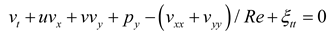
The structural dynamics governing equation for the motion of the cylinder is given by:
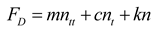
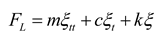 where FD and FL denote the drag and lift forces acting on the cylinder; m signifies the mass of the cylinder; c and k represent the damping and stiffness of the cylinder.
After reconstructing the velocity and pressure fields, the lift and drag forces acting on the cylinder can be inferred from the velocity gradients and the pressure field, as expressed in the following equation:
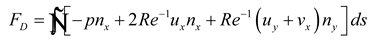
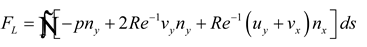 where nx and ny are the outward normal components of the cylinder's surface; ds is the arc length of the cylinder's surface.
2.2. Physics-Informed Neural Network (PINN)
A PINN is essentially a deep neural network (DNN) augmented with physical prior knowledge, enabling it to accurately approximate any continuous function. In the training of a PINN, partial differential equations (PDEs) residuals at specified points in the computational domain, along with the initial and boundary conditions are added to the loss function. This ensures that the predicted results align with the prior knowledge embedded in physical laws. The training of a PINN is not only data driven, but also constrained via physical principles, thereby enhancing the model's precision and reliability. Compared to traditional DNNs, PINNs reduce dependence on the training dataset, enhance the interpretability of the network model, and demonstrate superior generalization capabilities. Leveraging the widely-used automatic differentiation technique in DNNs, PINNs can accurately compute the derivatives of network outputs with respect to input variables, which facilitates the calculation of the PDE residuals to serve as physical constraints.
The objective of this research is to build the flow field of two-dimensional VIV, and predict the displacement of a cylindrical structure in the absence of flow field pressure data. The physical prior knowledge of PINN consists of the continuity equation and the momentum conservation equation (Navier-Stokes equations) for incompressible fluids, as shown in equations (1a), (1b), and (1c). Here, , , and represent the residuals of the three physical equations, as detailed below.


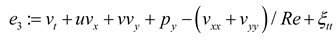 where, x and y are spatial variables; t is the time variable. The velocity and pressure of the flow field, with respect to spatial and temporal derivatives, are nonlinear differential operators, which are computed by the neural network through automatic differentiation techniques.
The structure of the PINN used for two-dimensional VIV of a cylindrical body is displayed in Figure 2, where the physical constraints of the continuity equation and the Navier-Stokes equations are incorporated into a fully connected network. The network architecture employed in this research is built upon the design proposed by Cheng et al. [35]. The PINN consists of a 14-layer neural network, encompassing an input layer, an output layer, as well as 12 hidden layers, with each hidden layer containing 64 neurons. The network weights are initialized via Xavier initialization, while the biases are initialized to 0. The activation function chosen is the sine function to introduce nonlinearity. The inputs to the network include spatial coordinates (x,y) and time t, and the outputs of the network are the downstream velocity u, lateral velocity v, pressure p of the flow field, and the downstream displacement and lateral displacement of the cylindrical body. The loss function is composed of two components: the data loss and the equation loss. The data loss is the error between the predicted values of the neural network and the data set, which includes four components: downstream velocity u, lateral velocity v, downstream displacement n, and lateral displacement r. By calculating the network outputs and various partial derivatives, we substitute these results into the governing equations, which allows us to compute the equation losses , , and of the partial differential equations. The PINN loss function is as follows:
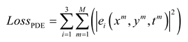
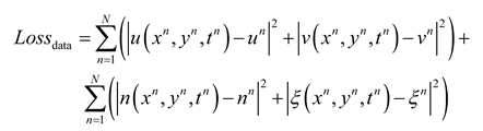 where N is the number of training data points in the dataset; M is the number of configuration points for the equation losses. represents the data loss, and represents the equation losses for the three physical equations.
2.3. GradNorm Algorithm
The loss function of the PINN encompasses both data loss and the residual losses of different physical equations. The gradients of these different losses during backpropagation can vary significantly, which may lead the model to focus disproportionately on certain losses while neglecting others. This can lead to poor convergence speed of the model as well as inadequate performance of the model in prediction. In order to elevate the model's learning capacity, we need to properly weight these different losses, which means we need to balance their gradients, and make the training more uniform. As a result, the multi task learning algorithms from computer vision can be utilized during the training of the PINN to increase the stability of the network model.
In multi-task learning, simply summing the losses of varying tasks to form the total loss does not account for the varying contributions of each task's backpropagation gradients to the network model. When there are significant discrepancies between the gradients of different tasks, those with smaller gradients may not receive sufficient learning, preventing a balance in the losses across tasks. Introducing fixed weights in the loss function can help balance these gradient differences, but assigning small weights to high gradient tasks will unnecessarily limit the learning of tasks, which ultimately impedes the effective learning of tasks with larger gradients. To solve this issue, in multi-task learning optimization, regarding the task weights as trainable parameters enables the model to automatically adjust the weights during training in response to variations in task gradients, ensuring a more balanced learning process for all tasks.
In this study, we propose a PINN with adaptive weights for solving the vortex-induced vibration problem, building on the GradNorm algorithm for multi-task optimization in computer vision [46]. The GradNorm algorithm adjusts the weight of each task dynamically in the process of training, so that the contributions of varying loss components in the overall loss function are balanced, making the model learn each task more evenly. In particular, the GradNorm algorithm compares the actual gradient norm of a task with the target gradient norm of each task, and accordingly scales the task weights. When the actual gradient norm of a task exceeds the target gradient norm, the algorithm reduces the weight of that task, allowing tasks with larger actual gradients to receive smaller weights, while tasks with smaller gradients are assigned larger weights. This approach allows the model to balance gradient norm across all tasks, so that all tasks learn at a similar rate. The implementation of the GradNorm algorithm’s loss function is as follows:
In the algorithm, the multi task loss function is a linear function of the single-task losses, and the loss function is as follows:
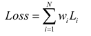 where N is the number of tasks, w and Li are the single-task weights and losses.
The gradient norm of the weighted loss for a single task is as follows:
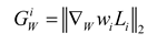 where signifies the gradient norm of the weighted loss with respect to the network weights , and is a subset of the neural network weights. To save computational resources, the weights of the last shared layer are selected.
The average gradient norm is the mean value of the gradient norms across all tasks, given by:
The loss ratio and relative inverse training rate for a single task at the t-th iteration are:
 Where is the loss of task i at the t-th iteration; is the initial loss of task i.
The average gradient norm serves as the scaling factor for the gradient norms of different tasks, allowing the relative size of the gradients to be determined. The relative inverse training rate of a task helps balance the task gradients. If is larger, the training speed of the task will be slower, so the weighted gradient of the task should be higher to accelerate the task's training speed. The loss function of GradNorm is the sum of the L1 norms of the differences between the actual gradient norms and the target gradient norms of all tasks, as shown in the following equation:
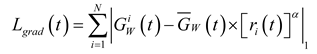 where is the target gradient norm for task i, and is a network hyperparameter representing the strength of the adjustment to align the tasks with the average training rate. The larger is, the stronger the constraint on the balance of the training rate.
After the loss function for the weights is obtained, is calculated, and the task weights are updated using backpropagation. After each weight update, the weights are re-normalized by setting .
2.4. Adaptive Weight Physics-Informed Neural Network (AW-PINN)
Building on the work presented in this study, we introduce an improved version of the GradNorm algorithm, which is applied as a multi-loss training method for PINNs. The proposed model, AW-PINN, automatically adjusts the weights of each task during training, ensuring that the learning rates are balanced across tasks without favoring any single one. By adopting this approach, we enhance the overall capability of the model to learn effectively. The implementation of AW-PINN is outlined as follows.
The task losses following the initialization of a PINN exhibit considerable uncertainty. Directly employing the initial task losses as for computing the relative inverse training rates may prevent the algorithm from accurately determining these rates, leading to significant uncertainty in the performance of AW-PINN. To address this, we perform pre-training with equal weights before applying the GradNorm algorithm, which makes the network achieve a stable initialization. Employing task losses after pretraining, represented as , effectively reduces the performance uncertainty caused by initialization. Moreover, appropriate pre-training can improve the model’s learning ability and enhance its predictive performance.
In the GradNorm algorithm, the task weights are updated by computing and then employing backpropagation to update the weight of task i. This weight update approach does not impose any constraints on the sign of the weights. However, in AW-PINN, the weights may become negative, resulting in negatively weighted task losses that adversely affect the model's training process. To ensure that the task weights remain positive throughout training, we define the weights as an exponential function, as follows:

 where is an intermediate value representing the task weight. By computing , and updating for task during backpropagation, the updated task weight can be obtained. The total sum of task weights is normalized to the number of tasks using Eq. (15), ensuring that the influence of individual tasks remains balanced during training and preventing any imbalance issues. The AW-PINN algorithm is summarized in Algorithm 1.
| Algorithm 1. Adaptive Weight Optimization Algorithm for PINN (AW-PINN) |
|
Step 1: Initialization Initialize network weights and biases Initialize task weights . Select the value of α and designate the shared layer (the last hidden layer). Step 2: Pre-training with Equal Weights For iteration from the first to the n-th iteration: Calculate . Train the network with equal weights. Step 3: Training with Adaptive Weighting Method At the n-th iteration, proceed as follows: Compute the total loss Calculate , ,, and . Compute Compute , and Update the loss weights with , and update the network weights using . Set ), and re-normalize . End. |
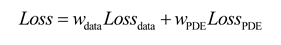
The AW-PINN model architecture is illustrated in Figure 3. After completing the PINN training, the data loss and equation loss are obtained. The hidden layers of the network serve as shared layers, with the last hidden layer selected to compute the gradient norm loss. This loss is then used to update the task weights for the subsequent iteration. The loss function of AW-PINN is as follows:
3. Results and Discussion
3.1. Obtaining the Training Dataset
To obtain a high-resolution dataset, a simulation analysis of the two-degree-of-freedom (2-DOF) VIV model of a cylinder was conducted. The simulated data were then selected as the training data for the neural network. As illustrated in Figure 4, the computational domain of the model is a rectangular region with a length of 40D and a width of 20D, where D is the diameter of the cylinder, and the initial position of the cylinder's center is at the origin of the coordinate system. The inlet boundary condition is a velocity inlet, located 10D from the cylinder's center. The outlet boundary condition is a pressure outlet, positioned 30D from the cylinder's center. The upper and lower side walls are treated as slip walls, each situated 10D from the cylinder's center, with a Reynolds number of Re=150, a fluid density of ρ=1.5kg/m3, and an inlet velocity of U=1m/s.
The flow field varies with changes in the cylinder's boundary. To simulate the motion of the cylinder boundary within the flow field, a nested grid technique[47] was employed. Based on the fluid simulation software and structural dynamics principles, a 2-DOF elastic-supported cylinder structure VIV numerical model was developed via User-Defined Functions (UDFs) and the nested grid technique. The nested grid around the cylinder was first divided into a foreground grid, which encloses the cylinder, and a background grid covering the flow field. Subsequently, the overlapping regions between the foreground grid boundary and the background grid were removed and interpolated. The foreground and background grids were then integrated into a coupled grid system, as depicted in Figure 5.
As presented in Table 1, to validate the reliability of the simulation results, we compared the simulation data with the findings from Bao et al. [48], including the transverse displacement , the downstream displacement , the root mean square value of the lift coefficient , and the average value of the drag coefficient . The errors between the two sets of results are minimal, confirming that the simulation results are suitable for use as the neural network dataset. The displacements in the x- and y-directions from the simulation results exhibit periodic variations, with the amplitude stabilizing after the fluctuations. Consequently, the simulation results are considered appropriate for training the neural network. For the 15-second simulation data, 150 snapshots of the flow field were selected, with a time interval of 0.1 seconds between consecutive snapshots. Flow field data within the coordinate range x∈[-2D,8D] and y∈[-4D,4D] were extracted, and 40,000 random samples were chosen from the flow field data as the training dataset.
3.2. Reconstructing the Flow Field Using Velocity Data
In the VIV problem of the cylinder, four models were employed to predict the flow field, as detailed in Table 2 These four models share the same network architecture and learning rate to compare their performance and stability. The PINN loss function is trained with equal weights. LB-PINN is a loss-balancing algorithm based on "uncertainty" that adjusts the weighting of losses. GNPINN leverages the backpropagated gradients of the weighted losses to balance the training speed of different weighted losses. By modifying the loss weights, it regulates the contributions of each loss to the overall loss function. AW-PINN optimizes the PINN using the GradNorm algorithm from multi-task learning, incorporating pre-training and improvements to limit negative weights.
The fixed weights for the PINN model were set to , while the initial weights for LB-PINN, GNPINN, and AW-PINN were also initialized to . All models were trained for 600 epochs, with 100 iterations per epoch. The initial learning rate of the network model was 0.002. For the first 200 epochs, the learning rate remained 0.002, after which it decayed to 0.1 times the previous value every 200 epochs.
Figure 6 illustrates the variations in the data loss weight and the equation loss weight throughout the training process. At the outset of training, the equation loss weight in LB-PINN rapidly increases to approximately 100, causing the loss function to be dominated by the data loss and impeding its convergence. In contrast, GNPINN and AW-PINN exhibit opposite trends in their weights. After 5000 iterations, GNPINN nearly disregards the data loss, with approaching 0. Conversely, AW-PINN tends to prioritize the training data loss, with both and converging to . Figure 7 depicts the changes in the training loss and test error for the four models during the training process. Throughout training, PINN and AW-PINN effectively reduce the training loss, demonstrating robust performance, with final training losses of 7.8×10⁻³ and 9.7×10⁻³, respectively. On the test set, AW-PINN achieves a 29% reduction in test error compared to PINN. However, both models exhibit signs of overfitting in the final 200 epochs, with the test error increasing abruptly upon learning rate adjustment. LB-PINN struggles to effectively train and minimize the loss function. GNPINN performs poorly, with a training loss of 1.8×10⁻² and a test error twice that of PINN.
Figure 8, Figure 9, Figure 10 and Figure 11 present the velocity and pressure fields predicted by the four network models, along with the errors between the numerical simulations and the model predictions. LB-PINN fails to accurately predict the flow field velocity and pressure, resulting in significant prediction errors. GNPINN provides relatively accurate predictions but still exhibits considerable errors. PINN and AW-PINN effectively infer the velocity and pressure fields across the entire flow field with reasonable accuracy, with AW-PINN providing the most precise predictions. Table 3 lists the mean squared errors (MSE) for various predictions of the four models on the validation set. PINN and AW-PINN achieve velocity field prediction accuracies on the order of 10-3, while LB-PINN and GNPINN converge only to the order of 10-2, with LB-PINN's downstream velocity MSE reaching 0.105. For the pressure field, PINN, AW-PINN, and GNPINN achieve prediction accuracies on the order of 10-3, whereas LB-PINN converges to 4.23×10⁻². All four models provide reasonably accurate predictions for the displacement of the cylindrical structure, with accuracies approximating 10-4. Figure 12 shows the predicted and simulated displacement values of the cylindrical structure. Compared to the simulation values, GNPINN's predicted peak displacement is approximately 7% higher, while the other three models exhibit relatively accurate prediction accuracy.
3.3. Stability Verification of AW-PINN
To assess the stability of the optimization algorithm, we trained the four models using the dataset from Raissi et al. [34]. This dataset consists of simulated data for a single-degree-of-freedom (1-DOF) cylinder undergoing VIV, analyzed via Direct Numerical Simulation (DNS). After the cylinder's vibration stabilized, flow field data from 280 time steps were recorded, with a time interval of 0.05 seconds between consecutive steps, spanning a total duration of 14 seconds.
Figure 13 presents the variations in the data loss weight and equation loss weight throughout the training process. Before 5000 iterations, LB-PINN tends to prioritize the equation loss in training; however, beyond this point, the data loss weight becomes slightly dominant. Both GNPINN and AW-PINN focus primarily on training the data loss, though during the first 1500 iterations, GNPINN tends to emphasize the equation loss. Figure 14 illustrates the loss function curves and test set error curves for the four models during the training process. In terms of training loss convergence performance, all four models exhibit similar trends, effectively reducing the loss values to the order of 10-4. Among the four network models, PINN exhibits the highest test error, while GNPINN and AW-PINN show comparable prediction errors, both lower than those of the other two models.
Figure 15, Figure 16, Figure 17 and Figure 18 depict the velocity and pressure fields predicted by the four network models, along with the errors between the numerical simulations and model predictions, using the 1-DOF dataset. In the velocity field prediction, PINN exhibits the largest maximum absolute error among the models, while the other three optimization algorithms demonstrate superior prediction performance. All models accurately predict the flow field pressure. Table 4 lists the mean squared errors for the four models on the validation set. The MSE for both the velocity field and structural displacement predictions across all models reaches the order of 10-5 Three of the optimization algorithms achieve an MSE for the flow field pressure on the order of 10-5, while PINN has an MSE of 1.35×10⁻⁴.
Figure 19 shows the structural displacement predictions and simulation values for the four models. All models accurately predict the cylindrical structure's displacement. Figure 20 compares the lift and drag inferred from the pressure field by the four models with the simulation results. In drag prediction, all four models exhibit high accuracy, with peak value error not exceeding 4%. Among them, AW-PINN performs best, with a maximum peak error of 1.4%. In lift prediction, PINN and LB-PINN exhibit larger prediction errors, with predicted lift deviating significantly at peak values, yielding maximum errors of 40.0% and 39.2%, respectively. GNPINN has a maximum peak prediction error of 22.7%, while AW-PINN demonstrates superior accuracy, with a maximum error of 8.2%. The network models in this study embed physical constraints into deep neural networks, regressing the training data while enforcing the corresponding partial differential equations. Due to the lack of training speed at and , the prediction accuracy for the start and end times in lift and drag predictions is relatively low, particularly for lift.
4. Conclusions
This study presents an Adaptive Weight Physics-Informed Neural Network (AW-PINN), designed to enhance the overall performance of the network model by adjusting the training speed of different loss terms, thereby balancing the model's learning process. The model optimizes the training speed of various loss terms by automatically adjusting the weight values, which in turn adapts the gradient magnitudes of the shared layers in the network. The study applies four models to different datasets and compares their results with numerical simulation data, leading to the following conclusions:
(1) The PINN model can utilize a limited amount of velocity data as the training set to accurately reconstruct the velocity and pressure fields of the VIV problem. Due to the absence of pressure data and the characteristics of the Navier-Stokes equations in the dataset, the pressure field reconstructed by PINN exhibits a constant difference in mean pressure compared to the numerical simulation results. However, it is capable of accurately predicting the distribution trend of the pressure. Additionally, the mean squared errors of the reconstructed velocity and pressure fields by PINN both converge to the order of 10-3.
(2) When addressing the single-degree-of-freedom vortex-induced vibration problem, both LB-PINN and GNPINN demonstrate strong performance. GNPINN achieves a mean squared error that is half of the PINN model in predicting the flow field velocity and structural displacement, and reduces the flow field pressure prediction error to one-third, significantly improving model performance. Although LB-PINN also enhances model performance, the improvement in flow field velocity prediction accuracy is limited. However, in the case of the two-degree-of-freedom VIV problem, both models tend to prioritize equation loss during training, resulting in larger prediction errors compared to PINN and failing to effectively address the two-degree-of-freedom VIV problem.
(3) Among all the models, AW-PINN exhibits the best performance in the single-degree-of-freedom VIV problem, significantly improving prediction accuracy. Compared to the other two optimization models, AW-PINN shows better stability in the two-degree-of-freedom VIV problem, as it tends to prioritize training data loss, significantly improving the prediction precision of flow field velocity and structural displacement, while also enhancing the prediction precision of the flow field pressure.
Although AW-PINN demonstrates superior performance compared to PINN, there are still some challenges to address. For example, AW-PINN requires the calculation of the loss gradient with respect to the network's shared layers, which increases the computational resources needed for training. Therefore, applying the network to large datasets and complex models using GPU parallel technology remains a challenge. Additionally, in practical applications, network models must balance multiple loss terms, necessitating further verification of the model’s performance and stability when managing multiple loss terms.
Author Contributions
Writing – review & editing, Validation, Supervision, Methodology, Investigation, Funding acquisition, Formal analysis, P.Z.; Writing - original draft, Visualization, Investigation, Formal analysis, Data curation, Conceptualization, Z.L. All authors have read and agreed to the published version of the manuscript.
Funding
This study was made possible with the support of Natural Science Foundation of Chongqing, China (CSTB2024NSCQ-MSX1206). The authors would like to express their gratitude for the financial supports.
Data Availability Statement
Data will be made available on request.
Conflicts of Interest
The authors declare that they have no known competing financial interests or personal relationships that could have appeared to influence the work reported in this paper.
References
- Matsumoto, M.; Yagi, T.; Shigemura, Y.; Tsushima, D. Vortex-induced cable vibration of cable-stayed bridges at high reduced wind velocity. Journal of Wind Engineering and Industrial Aerodynamics 2001, 89, 633–647. [Google Scholar] [CrossRef]
- Liu, Z.; Shen, J.; Li, S.; Chen, Z.; Ou, Q.; Xin, D. Experimental study on high-mode vortex-induced vibration of stay cable and its aerodynamic countermeasures. Journal of Fluids and Structures 2021, 100, 103195. [Google Scholar] [CrossRef]
- Kim, S.; Kim, S.; Kim, H.-K. High-mode vortex-induced vibration of stay cables: Monitoring, cause investigation, and mitigation. Journal of Sound and Vibration 2022, 524, 116758. [Google Scholar] [CrossRef]
- Chen, C.; Zhou, J.-w.; Li, F.; Gong, D. Nonlinear vortex-induced vibration of wind turbine towers: Theory and experimental validation. Mechanical Systems and Signal Processing 2023, 204, 110772. [Google Scholar] [CrossRef]
- Chizfahm, A.; Yazdi, E.A.; Eghtesad, M. Dynamic modeling of vortex induced vibration wind turbines. Renewable Energy 2018, 121, 632–643. [Google Scholar] [CrossRef]
- Han, X.; Lin, W.; Qiu, A.; Feng, Z.; Wu, J.; Tang, Y.; Zhao, C. Understanding vortex-induced vibration characteristics of a long flexible marine riser by a bidirectional fluid–structure coupling method. Journal of Marine Science and Technology 2020, 25, 620–639. [Google Scholar] [CrossRef]
- Hong, K.-S.; Shah, U.H. Vortex-induced vibrations and control of marine risers: A review. Ocean Engineering 2018, 152, 300–315. [Google Scholar] [CrossRef]
- Williamson, C.H.; Govardhan, R. Vortex-induced vibrations. Annu. Rev. Fluid Mech. 2004, 36, 413–455. [Google Scholar] [CrossRef]
- Kumar, N.; Kolahalam, V.K.V.; Kantharaj, M.; Manda, S. Suppression of vortex-induced vibrations using flexible shrouding—An experimental study. Journal of Fluids and Structures 2018, 81, 479–491. [Google Scholar] [CrossRef]
- Trim, A.; Braaten, H.; Lie, H.; Tognarelli, M. Experimental investigation of vortex-induced vibration of long marine risers. Journal of fluids and structures 2005, 21, 335–361. [Google Scholar] [CrossRef]
- Zhang, C.; Kang, Z.; Stoesser, T.; Xie, Z.; Massie, L. Experimental investigation on the VIV of a slender body under the combination of uniform flow and top-end surge. Ocean Engineering 2020, 216, 108094. [Google Scholar] [CrossRef]
- Wang, L.; Jiang, T.; Dai, H.; Ni, Q. Three-dimensional vortex-induced vibrations of supported pipes conveying fluid based on wake oscillator models. Journal of Sound and Vibration 2018, 422, 590–612. [Google Scholar] [CrossRef]
- Meng, S.; Chen, Y.; Che, C. Slug flow's intermittent feature affects VIV responses of flexible marine risers. Ocean Engineering 2020, 205, 106883. [Google Scholar] [CrossRef]
- Rahman, M.A.A.; Leggoe, J.; Thiagarajan, K.; Mohd, M.H.; Paik, J.K. Numerical simulations of vortex-induced vibrations on vertical cylindrical structure with different aspect ratios. Ships and Offshore Structures 2016, 11, 405–423. [Google Scholar] [CrossRef]
- Wu, W.; Wang, J. Numerical simulation of VIV for a circular cylinder with a downstream control rod at low Reynolds number. European Journal of Mechanics-B/Fluids 2018, 68, 153–166. [Google Scholar] [CrossRef]
- Gabbai, R.D.; Benaroya, H. An overview of modeling and experiments of vortex-induced vibration of circular cylinders. Journal of sound and vibration 2005, 282, 575–616. [Google Scholar] [CrossRef]
- Evangelinos, C.; Lucor, D.; Karniadakis, G. DNS-derived force distribution on flexible cylinders subject to vortex-induced vibration. Journal of fluids and structures 2000, 14, 429–440. [Google Scholar] [CrossRef]
- Chen, W.; Ji, C.; Xu, D.; Zhang, Z. Three-dimensional direct numerical simulations of vortex-induced vibrations of a circular cylinder in proximity to a stationary wall. Physical Review Fluids 2022, 7, 044607. [Google Scholar] [CrossRef]
- Wang, X.; Xu, F.; Zhang, Z.; Wang, Y. 3D LES numerical investigation of vertical vortex-induced vibrations of a 4: 1 rectangular cylinder. Advances in Wind Engineering 2024, 1, 100008. [Google Scholar] [CrossRef]
- Al-Jamal, H.; Dalton, C. Vortex induced vibrations using large eddy simulation at a moderate Reynolds number. Journal of fluids and structures 2004, 19, 73–92. [Google Scholar] [CrossRef]
- Pan, Z.; Cui, W.; Miao, Q. Numerical simulation of vortex-induced vibration of a circular cylinder at low mass-damping using RANS code. Journal of Fluids and Structures 2007, 23, 23–37. [Google Scholar] [CrossRef]
- Khan, N.B.; Ibrahim, Z.; Nguyen, L.T.T.; Javed, M.F.; Jameel, M. Numerical investigation of the vortex-induced vibration of an elastically mounted circular cylinder at high Reynolds number (Re= 104) and low mass ratio using the RANS code. PloS one 2017, 12, e0185832. [Google Scholar] [CrossRef] [PubMed]
- Dobrucali, E.; Kinaci, O. URANS-based prediction of vortex induced vibrations of circular cylinders. Journal of applied fluid mechanics 2017, 10, 957–970. [Google Scholar] [CrossRef]
- Liu, G.; Li, H.; Qiu, Z.; Leng, D.; Li, Z.; Li, W. A mini review of recent progress on vortex-induced vibrations of marine risers. Ocean Engineering 2020, 195, 106704. [Google Scholar] [CrossRef]
- Cuomo, S.; Di Cola, V.S.; Giampaolo, F.; Rozza, G.; Raissi, M.; Piccialli, F. Scientific machine learning through physics–informed neural networks: Where we are and what’s next. Journal of Scientific Computing 2022, 92, 88. [Google Scholar] [CrossRef]
- Mathew, A.; Amudha, P.; Sivakumari, S. Deep learning techniques: an overview. Advanced Machine Learning Technologies and Applications: Proceedings of AMLTA 2020 2021, 599–608. [Google Scholar]
- LeCun, Y.; Bengio, Y.; Hinton, G. Deep learning. nature 2015, 521, 436–444. [Google Scholar] [CrossRef]
- Lino, M.; Fotiadis, S.; Bharath, A.A.; Cantwell, C.D. Current and emerging deep-learning methods for the simulation of fluid dynamics. Proceedings of the Royal Society A 2023, 479, 20230058. [Google Scholar] [CrossRef]
- Jin, X.; Cheng, P.; Chen, W.-L.; Li, H. Prediction model of velocity field around circular cylinder over various Reynolds numbers by fusion convolutional neural networks based on pressure on the cylinder. Physics of Fluids 2018, 30. [Google Scholar] [CrossRef]
- Sekar, V.; Jiang, Q.; Shu, C.; Khoo, B.C. Fast flow field prediction over airfoils using deep learning approach. Physics of Fluids 2019, 31. [Google Scholar] [CrossRef]
- Kim, G.-y.; Lim, C.; Kim, E.S.; Shin, S.-c. Prediction of dynamic responses of flow-induced vibration using deep learning. Applied Sciences 2021, 11, 7163. [Google Scholar] [CrossRef]
- Xu, H.; Zhang, D.; Wang, N. Deep-learning based discovery of partial differential equations in integral form from sparse and noisy data. Journal of Computational Physics 2021, 445, 110592. [Google Scholar] [CrossRef]
- Raissi, M.; Perdikaris, P.; Karniadakis, G.E. Physics-informed neural networks: A deep learning framework for solving forward and inverse problems involving nonlinear partial differential equations. Journal of Computational physics 2019, 378, 686–707. [Google Scholar] [CrossRef]
- Raissi, M.; Wang, Z.; Triantafyllou, M.S.; Karniadakis, G.E. Deep learning of vortex-induced vibrations. Journal of Fluid Mechanics 2019, 861, 119–137. [Google Scholar] [CrossRef]
- Cheng, C.; Meng, H.; Li, Y.-Z.; Zhang, G.-T. Deep learning based on PINN for solving 2 DOF vortex induced vibration of cylinder. Ocean Engineering 2021, 240, 109932. [Google Scholar] [CrossRef]
- Tang, H.; Liao, Y.; Yang, H.; Xie, L. A transfer learning-physics informed neural network (TL-PINN) for vortex-induced vibration. Ocean Engineering 2022, 266, 113101. [Google Scholar] [CrossRef]
- Zhu, Y.; Yan, Y.; Zhang, Y.; Zhou, Y.; Zhao, Q.; Liu, T.; Xie, X.; Liang, Y. Application of Physics-Informed Neural Network (PINN) in the Experimental Study of Vortex-Induced Vibration with Tunable Stiffness. In Proceedings of the ISOPE International Ocean and Polar Engineering Conference, 2023; pp. ISOPE-I-23-305. [Google Scholar]
- Wang, S.; Teng, Y.; Perdikaris, P. Understanding and mitigating gradient pathologies in physics-informed neural networks. arXiv preprint, 2020; arXiv:2001.04536 2020. [Google Scholar]
- Xiang, Z.; Peng, W.; Liu, X.; Yao, W. Self-adaptive loss balanced physics-informed neural networks. Neurocomputing 2022, 496, 11–34. [Google Scholar] [CrossRef]
- Chen, Y.; Xu, Y.; Wang, L.; Li, T. Modeling water flow in unsaturated soils through physics-informed neural network with principled loss function. Computers and Geotechnics 2023, 161, 105546. [Google Scholar] [CrossRef]
- Tarbiyati, H.; Nemati Saray, B. Weight initialization algorithm for physics-informed neural networks using finite differences. Engineering with Computers 2024, 40, 1603–1619. [Google Scholar] [CrossRef]
- Li, S.; Feng, X. Dynamic weight strategy of physics-informed neural networks for the 2d navier–stokes equations. Entropy 2022, 24, 1254. [Google Scholar] [CrossRef]
- Hou, X.; Zhou, X.; Liu, Y. Reconstruction of ship propeller wake field based on self-adaptive loss balanced physics-informed neural networks. Ocean Engineering 2024, 309, 118341. [Google Scholar] [CrossRef]
- Shi, S.; Liu, D.; Huo, Z. Simulation of thermal-fluid coupling in silicon single crystal growth based on gradient normalized physics-informed neural network. Physics of Fluids 2024, 36. [Google Scholar] [CrossRef]
- Yin, G.; Janocha, M.J.; Ong, M.C. Physics-Informed Neural Networks for Prediction of a Flow-Induced Vibration Cylinder. Journal of Offshore Mechanics and Arctic Engineering 2024, 146. [Google Scholar] [CrossRef]
- Chen, Z.; Badrinarayanan, V.; Lee, C.-Y.; Rabinovich, A. Gradnorm: Gradient normalization for adaptive loss balancing in deep multitask networks. In Proceedings of the International conference on machine learning; 2018; pp. 794–803. [Google Scholar]
- Zhao, G.; Xu, J.; Duan, K.; Zhang, M.; Zhu, H.; Wang, J. Numerical analysis of hydroenergy harvesting from vortex-induced vibrations of a cylinder with groove structures. Ocean Engineering 2020, 218, 108219. [Google Scholar] [CrossRef]
- Bao, Y.; Huang, C.; Zhou, D.; Tu, J.; Han, Z. Two-degree-of-freedom flow-induced vibrations on isolated and tandem cylinders with varying natural frequency ratios. Journal of Fluids and Structures 2012, 35, 50–75. [Google Scholar] [CrossRef]
Figure 1.
Physical model of two-degree-of freedom (2-DOF) vortex-induced vibration
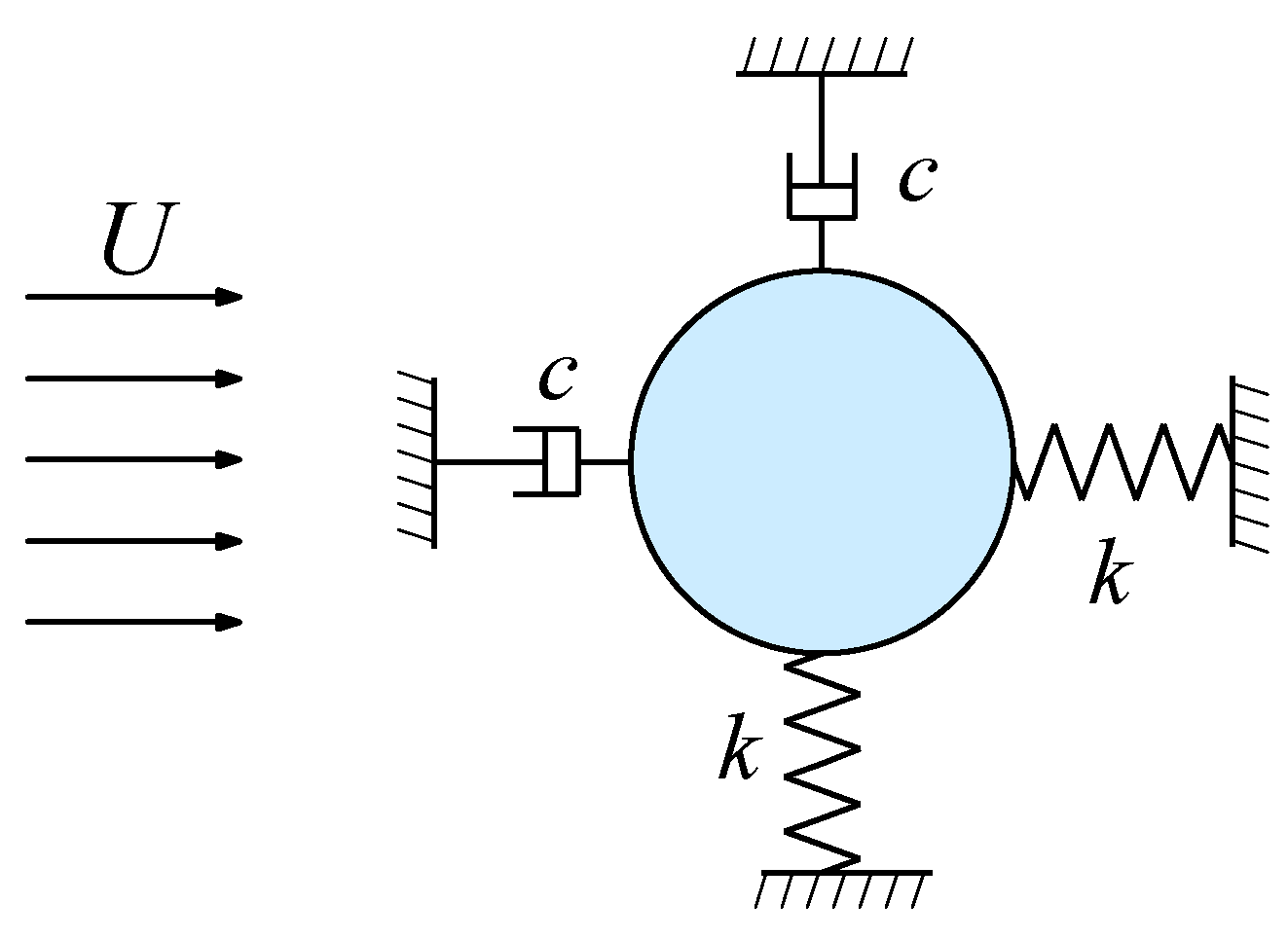
Figure 2.
Network architecture of PINN for solving vortex induced vibration problems
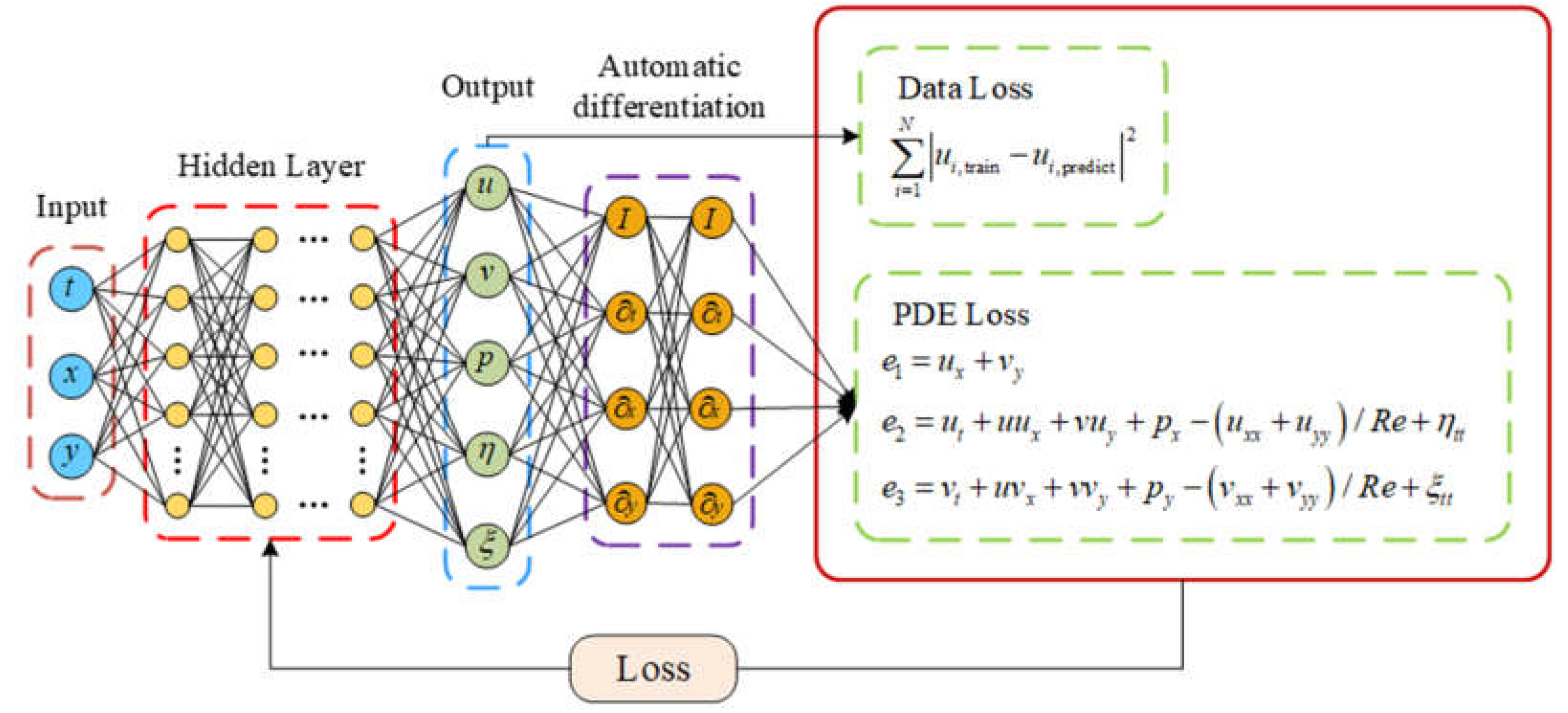
Figure 3.
Network architecture of AW-PINN for solving vortex-induced vibration problem
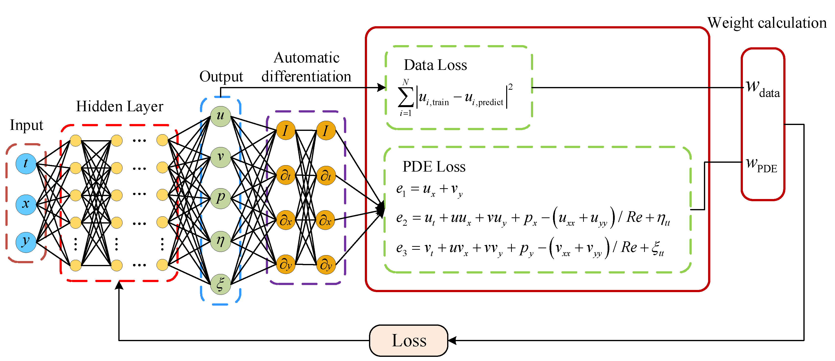
Figure 4.
Computational domain and boundary conditions of the flow field
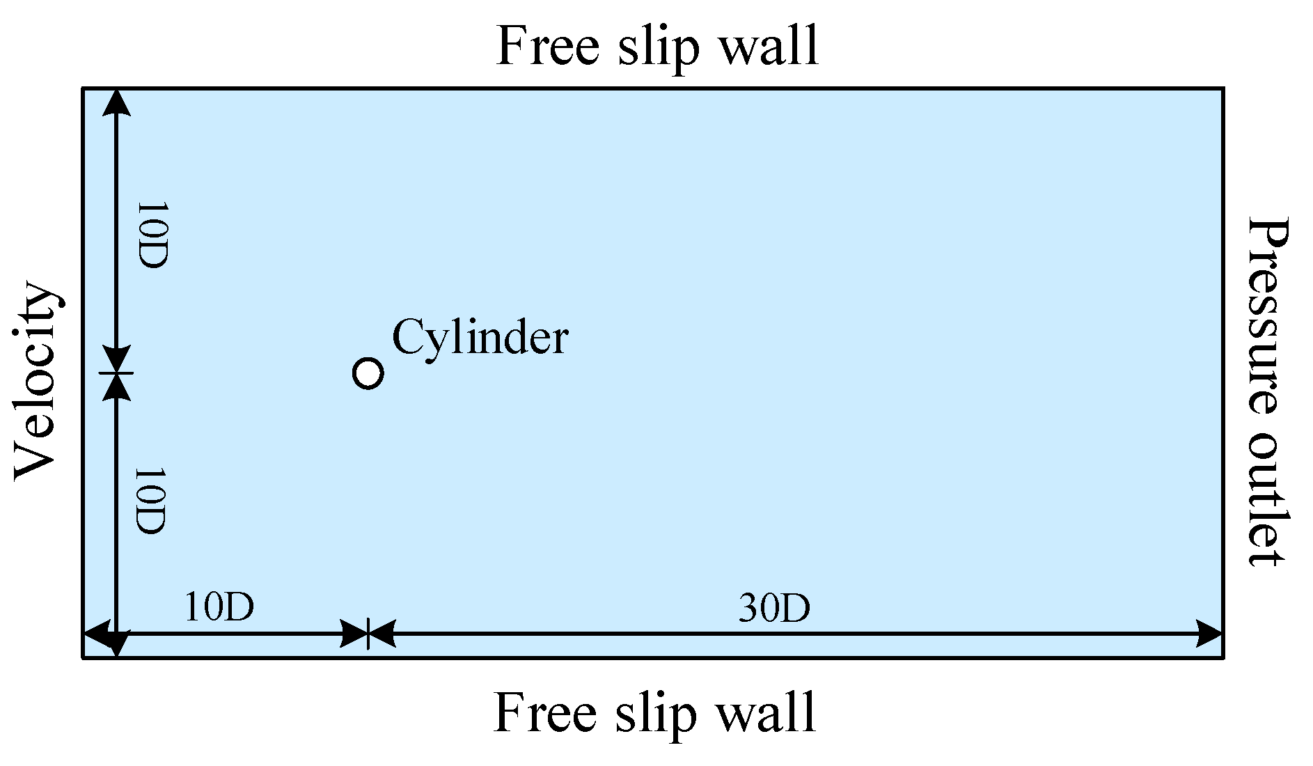
Figure 5.
Meshing for computational domains
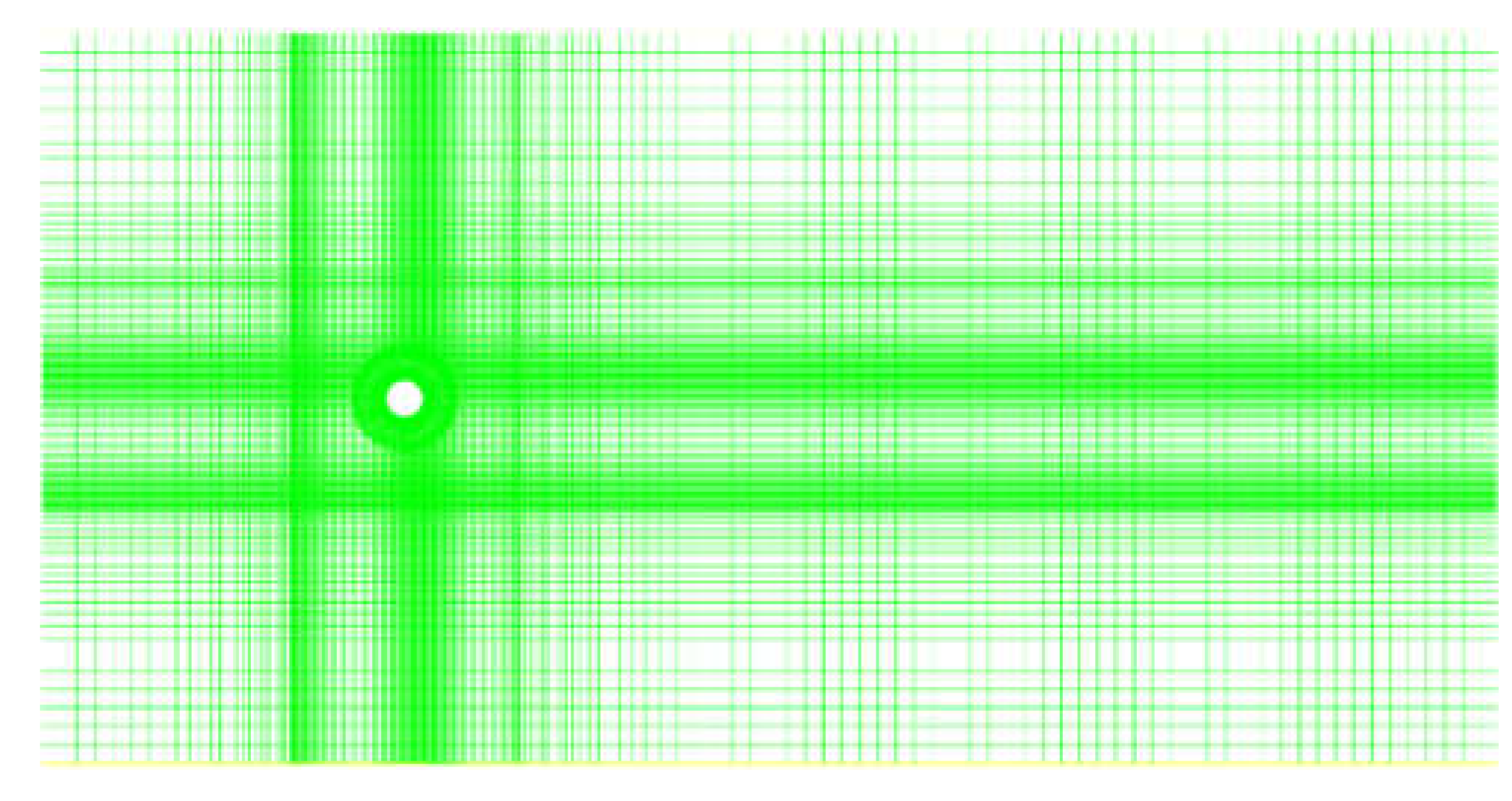
Figure 6.
Adaptive weight changes in the 2-DOF cylinder:(a) LB-PINN; (b) GNPINN; (c) AW-PINN
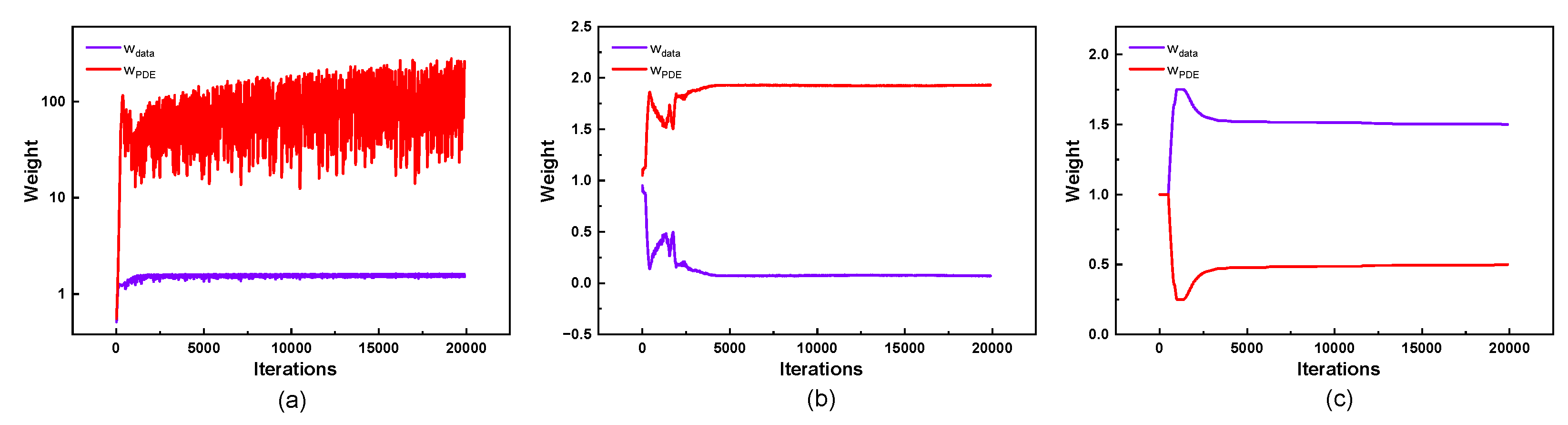
Figure 7.
Mean square error of four models in the 2-DOF cylinder:(a) Training loss curves; (b) Test error curves
Figure 7.
Mean square error of four models in the 2-DOF cylinder:(a) Training loss curves; (b) Test error curves
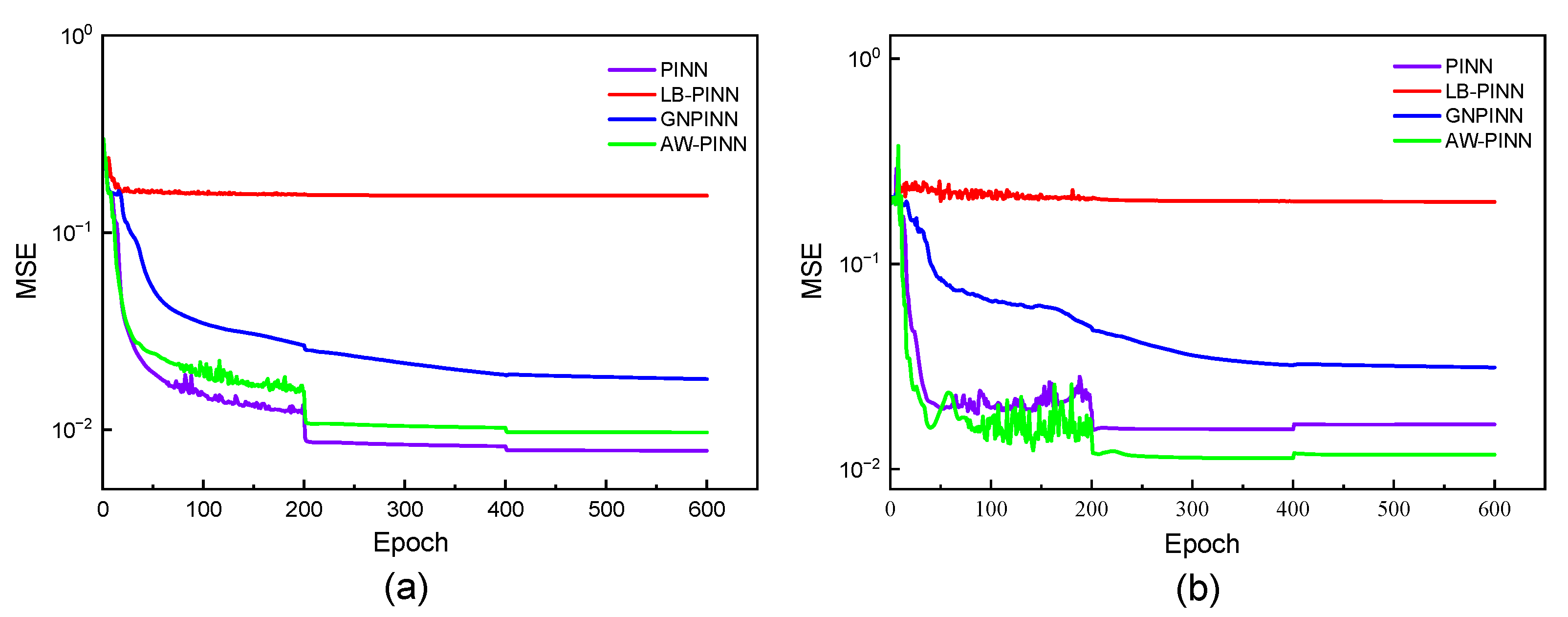
Figure 8.
Flow field prediction for PINN in the 2-DOF cylinder
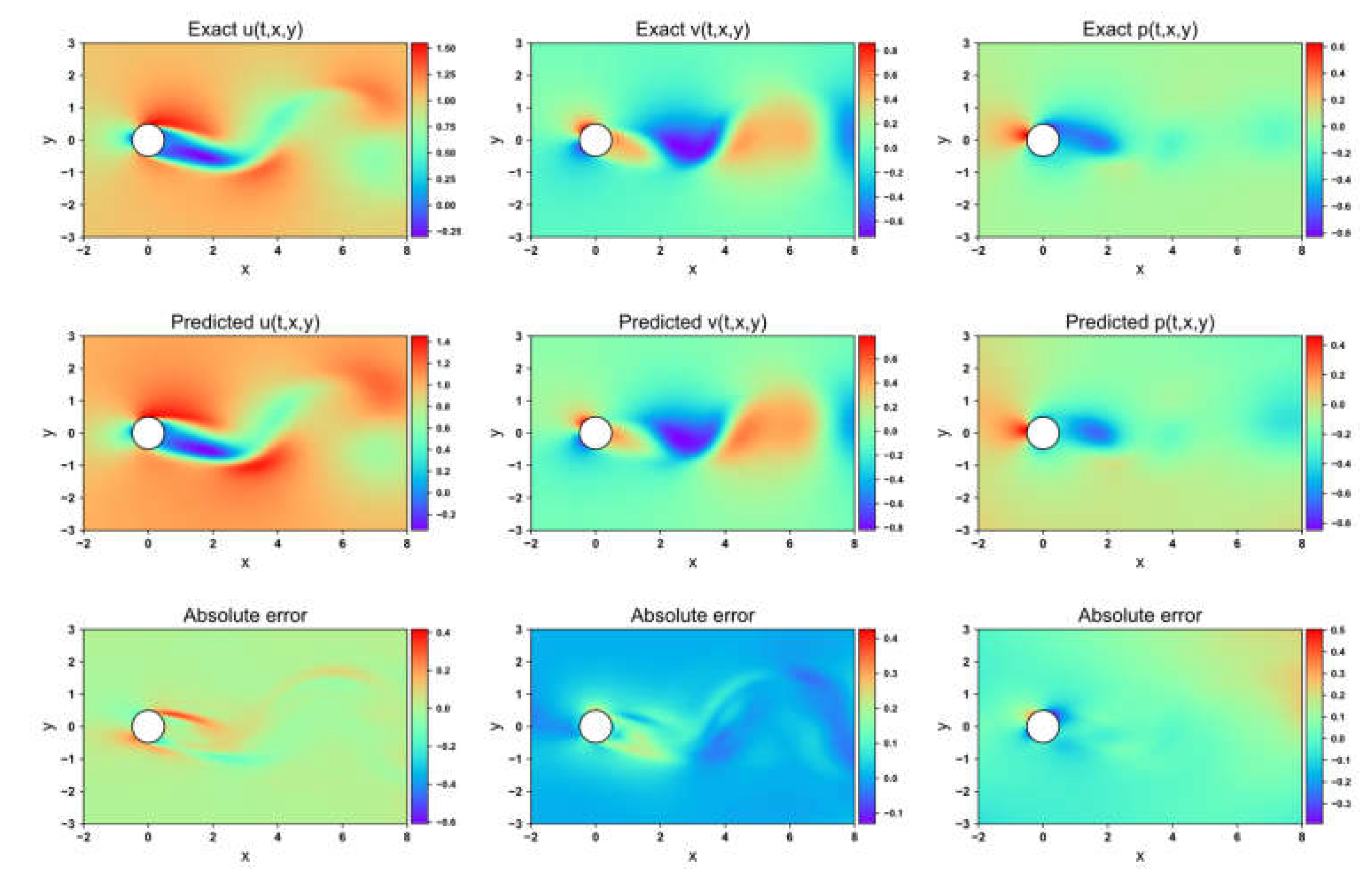
Figure 9.
Flow field prediction for LB-PINN in the 2-DOF cylinder
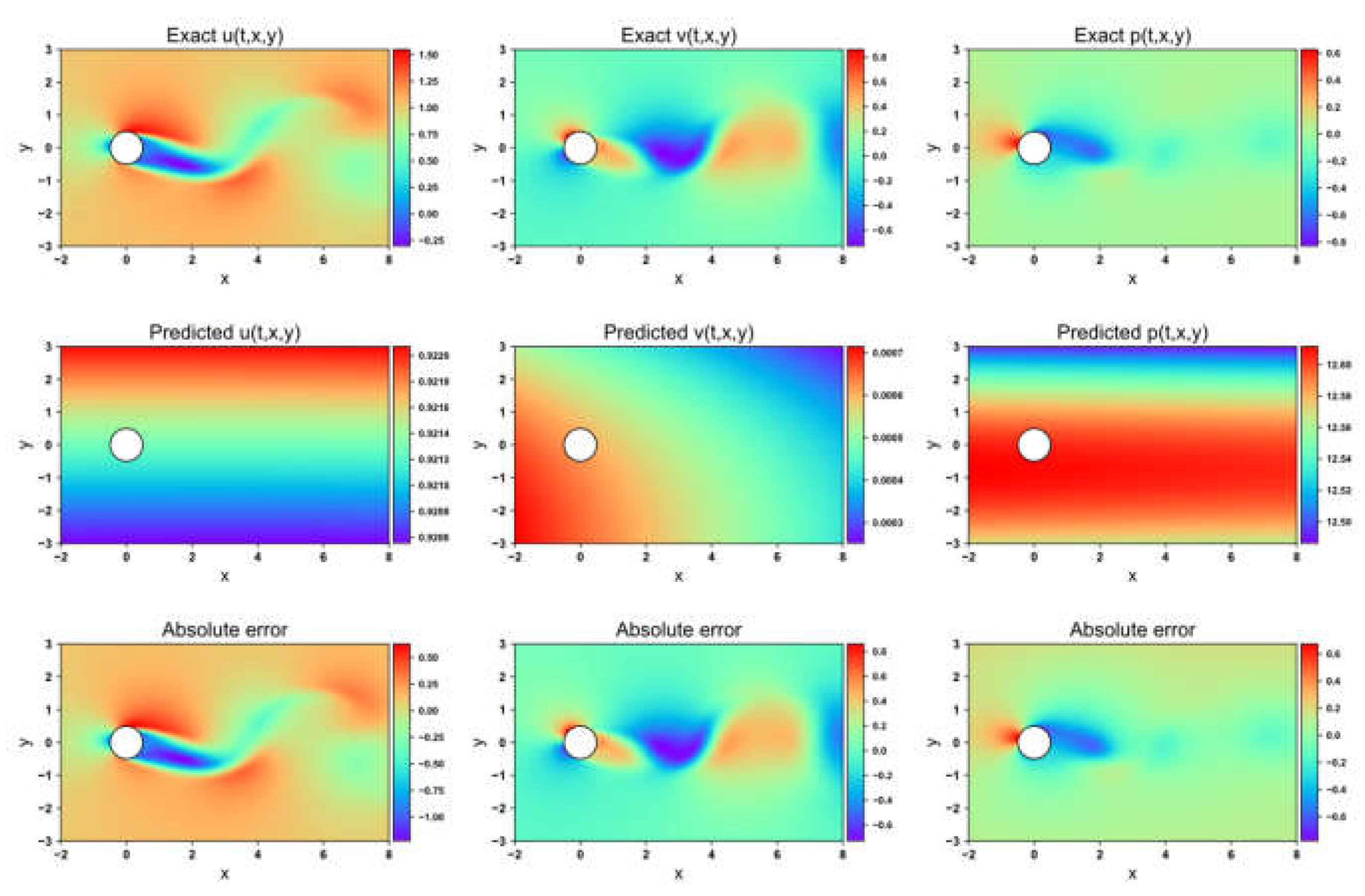
Figure 10.
Flow field prediction for GNPINN in 2-DOF cylinder
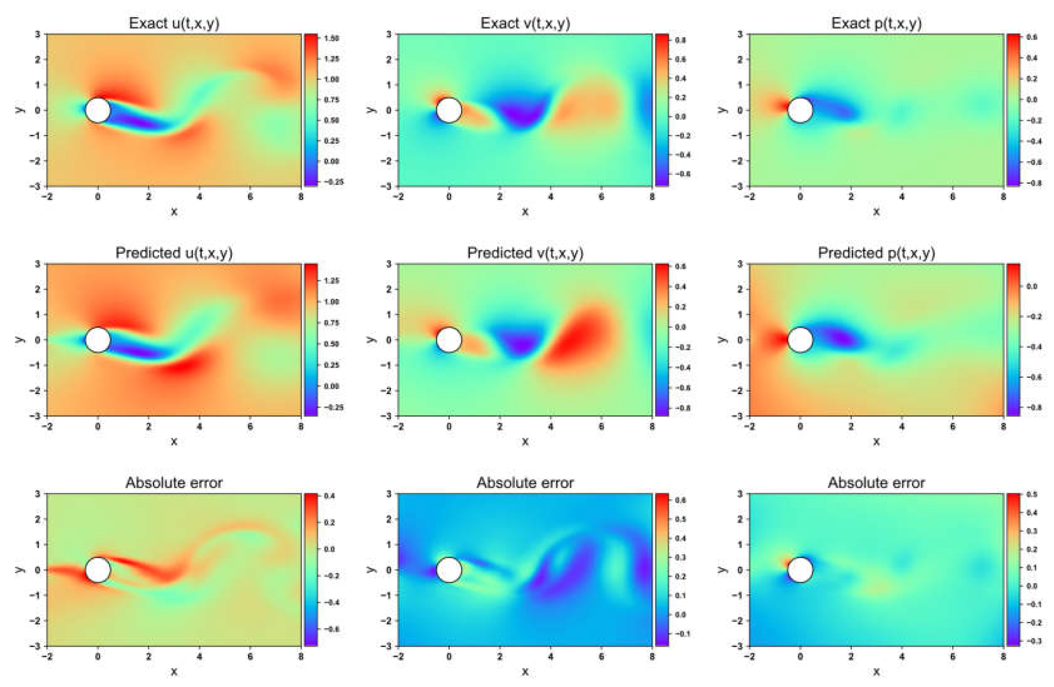
Figure 11.
Flow field prediction for AW-PINN in the 2-DOF cylinder
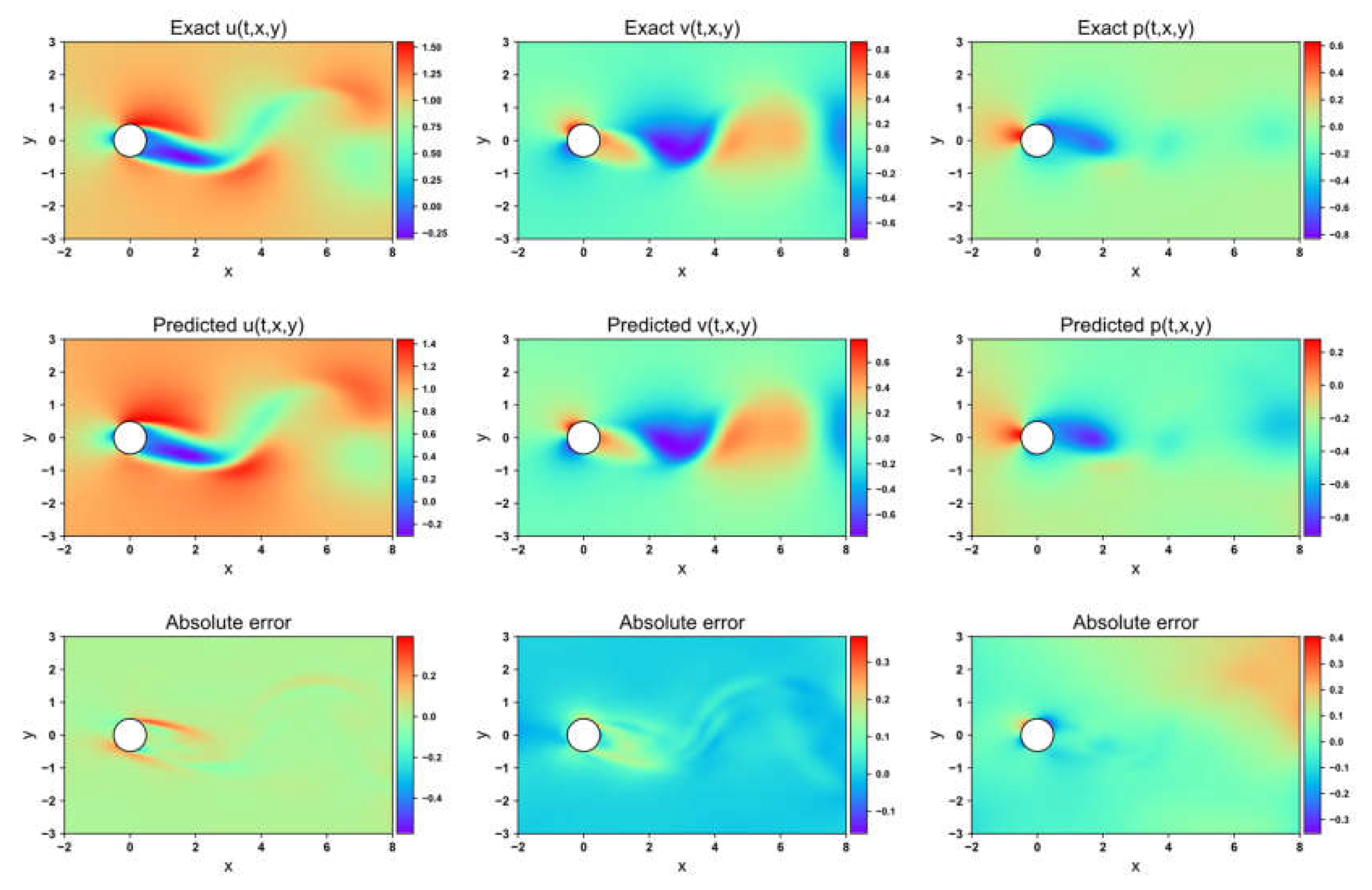
Figure 12.
Transverse structural displacement prediction in the 2-DOF cylinder
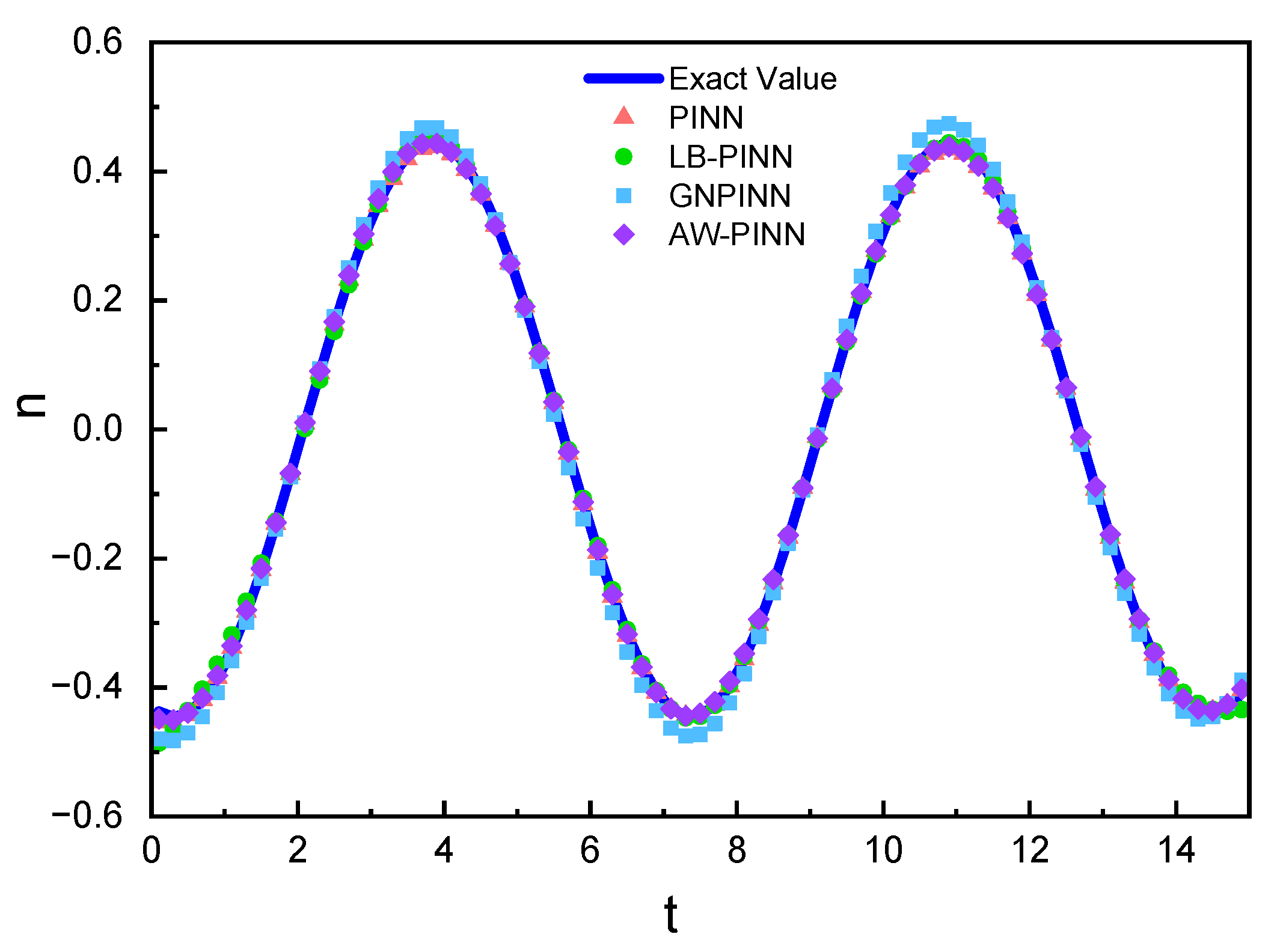
Figure 13.
Adaptive weight changes in the 1-DOF cylinder: (a) LB-PINN;(b) GNPINN;(c) AW-PINN
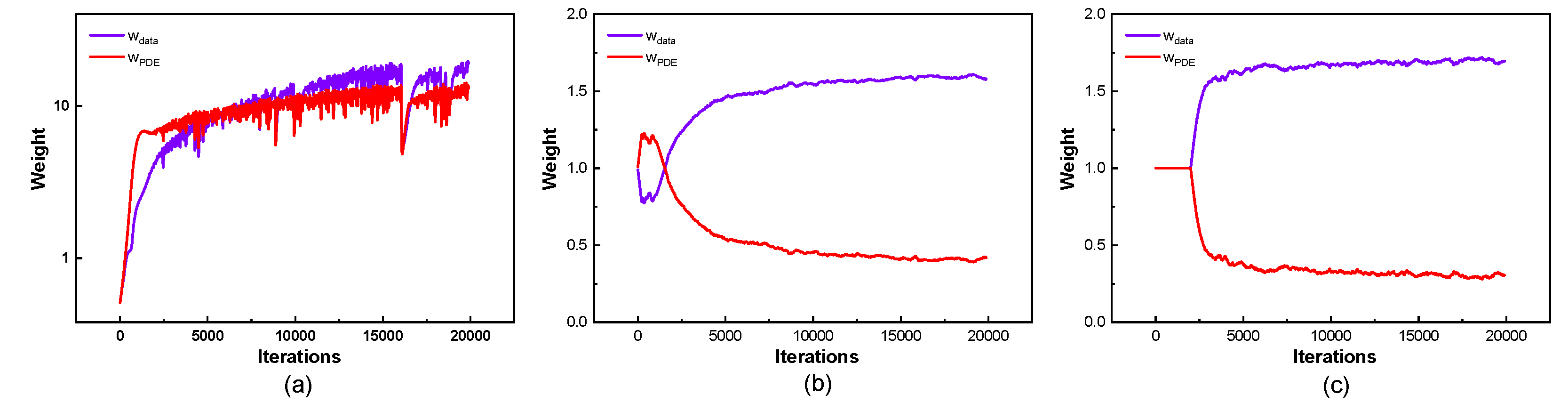
Figure 14.
Mean square error of four models in the 1-DOF cylinder:(a) training loss curves;(b) test error curves
Figure 14.
Mean square error of four models in the 1-DOF cylinder:(a) training loss curves;(b) test error curves
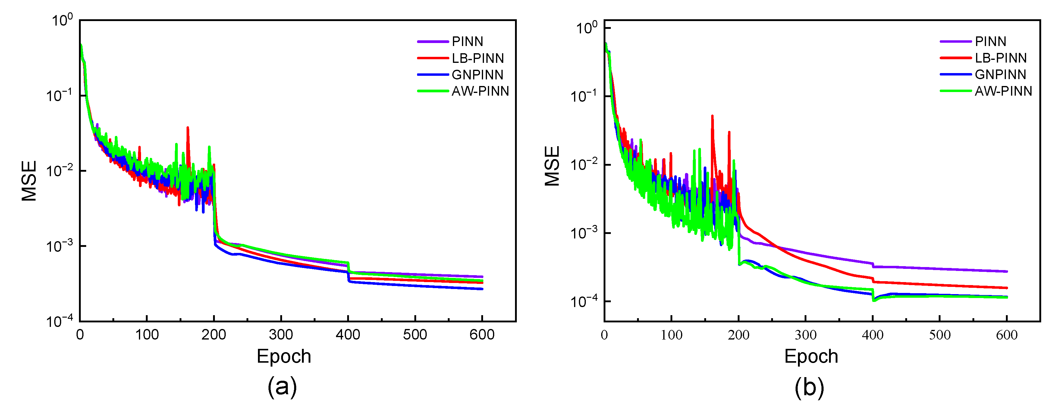
Figure 15.
Flow field prediction for PINN in the 1-DOF cylinder
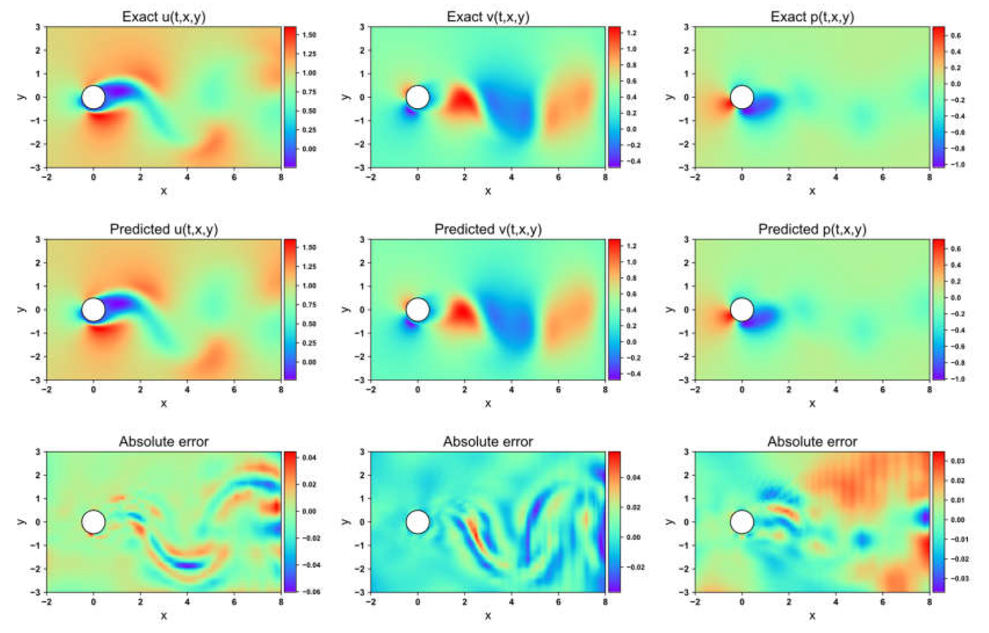
Figure 16.
Flow field prediction for LB-PINN in the 1-DOF cylinder
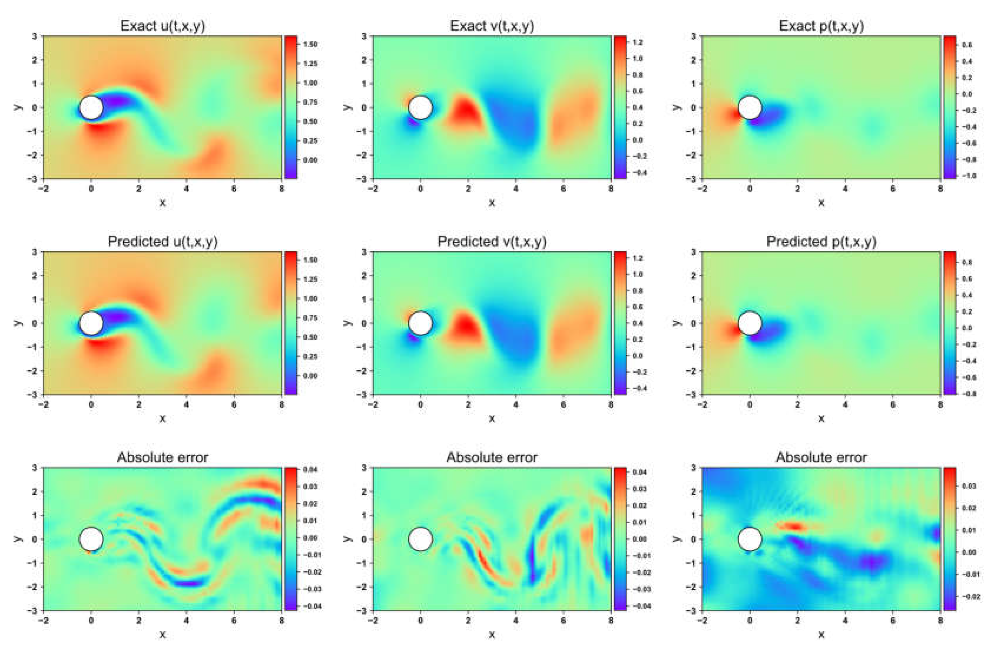
Figure 17.
Flow field prediction for GNPINN in 1-DOF cylinder
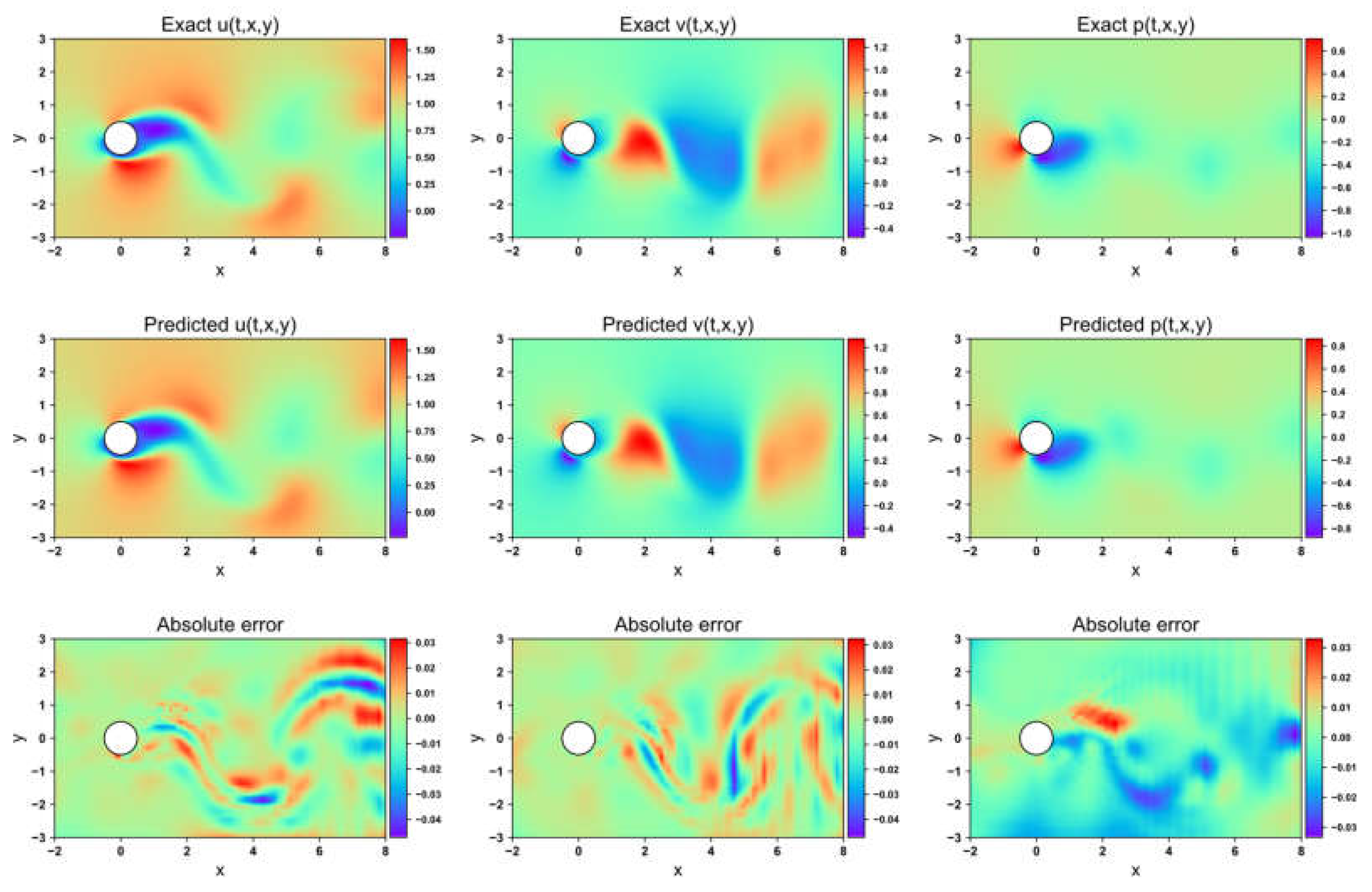
Figure 18.
Flow field prediction for AW-PINN in the 1-DOF cylinder
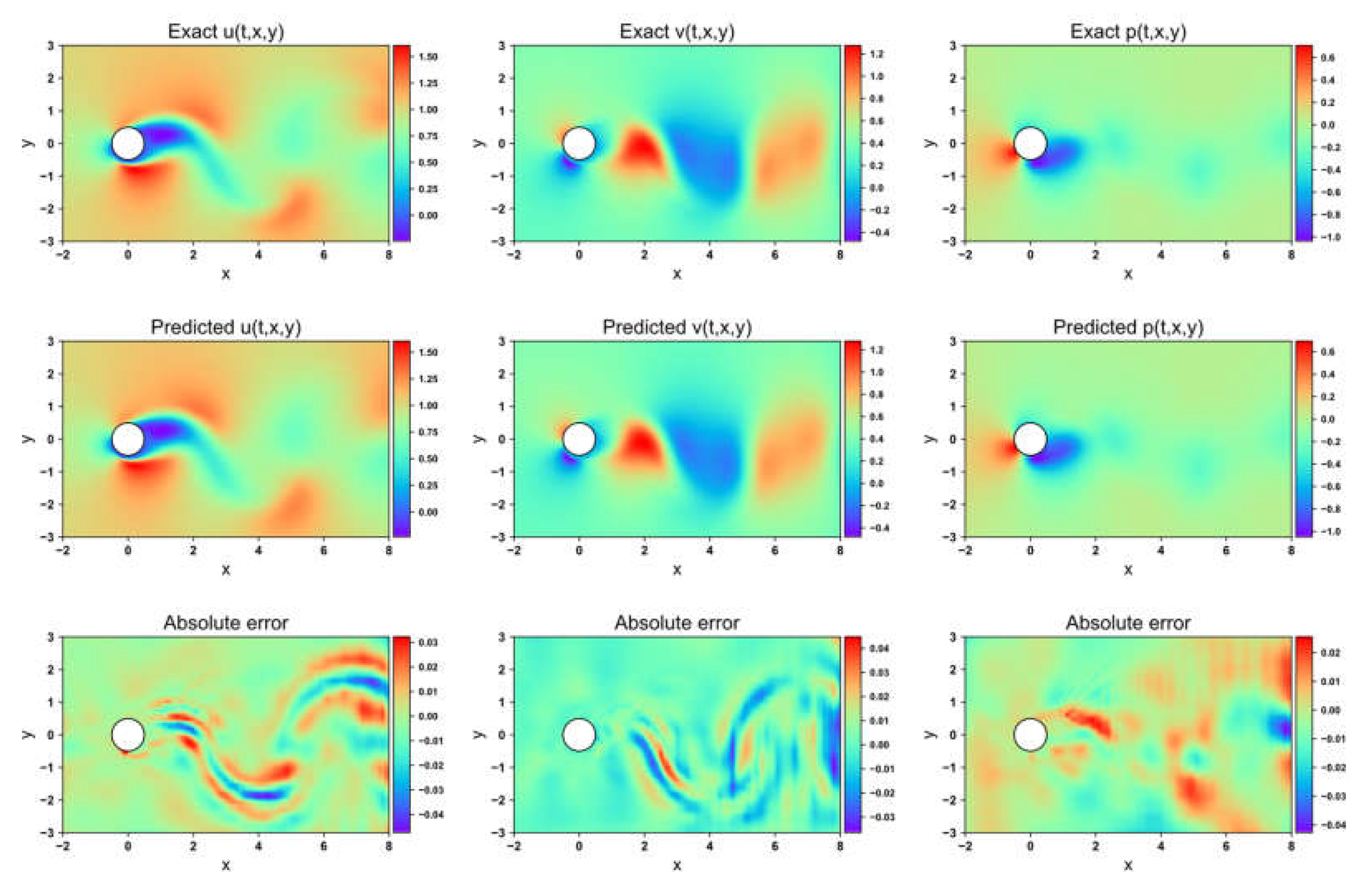
Figure 19.
Transverse structural displacement prediction in the 1-DOF cylinder.
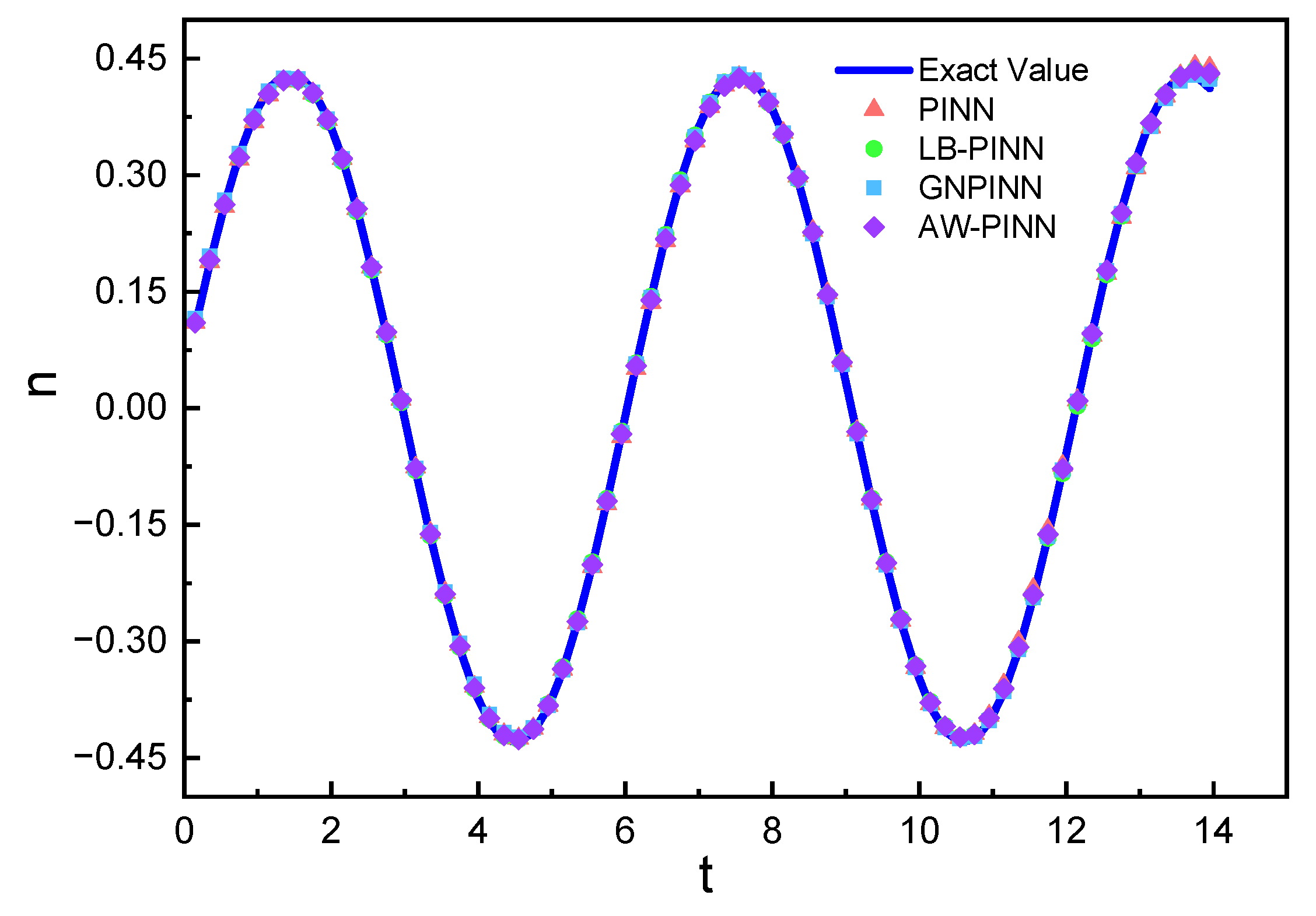
Figure 20.
Force prediction of cylinder:(a) drag of cylinder(b) lift of cylinder
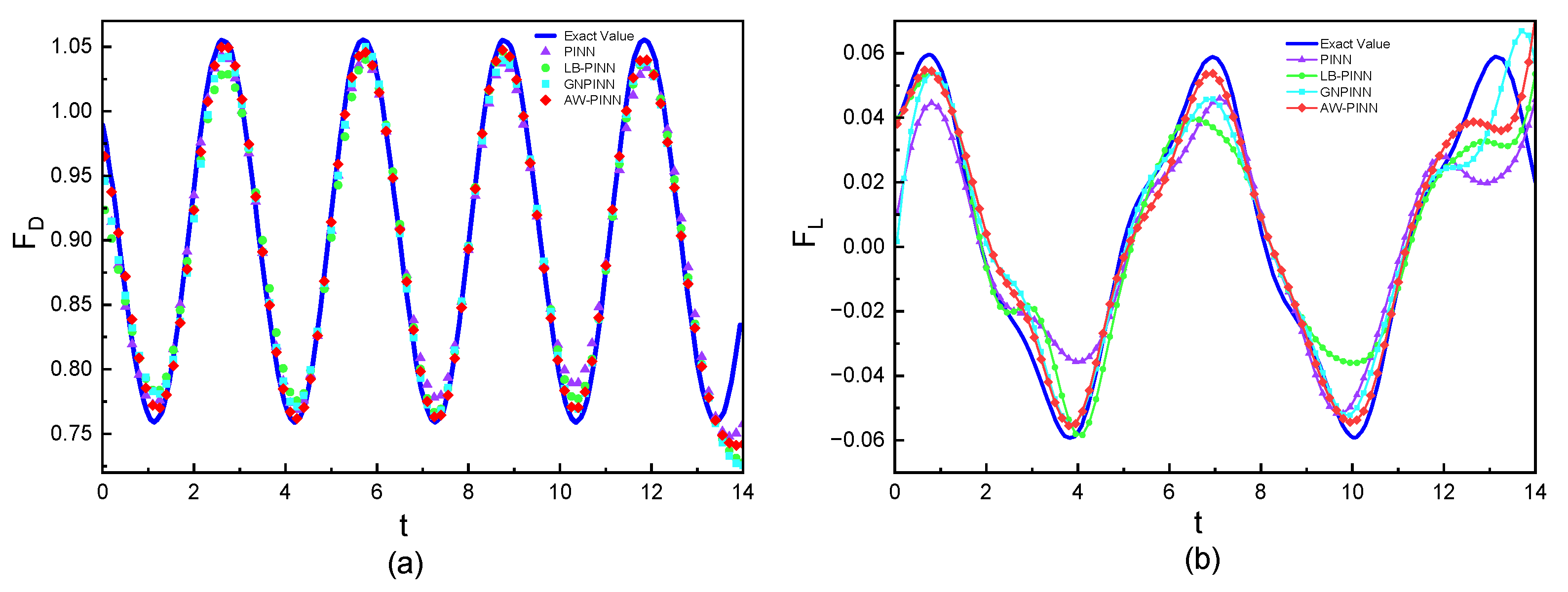

Table 1.
Comparison of numerical simulation results with other studies
| Numerical result | ||||
|---|---|---|---|---|
| Bao et al. | 0.030 | 0.61 | 0.29 | 2.03 |
| This study | 0.031 | 0.60 | 0.27 | 2.08 |
Table 2.
Overview of different models
| Model | Brief description of the model |
| PINN | The baseline PINN trained with an equal weight loss function.[34] |
| LB-PINN | The loss function is optimized using uncertainty to enhance PINN performance.[43] |
| GNPINN | Loss weights are adjusted based on gradient normalization to optimize PINN.[44] |
| AW-PINN | The PINN optimization method proposed in this study. |
Table 3.
Mean squared errors of predictions by different models
| Model | Mean Squared Error | ||||
|---|---|---|---|---|---|
| u | v | p | n | r | |
| PINN | 3.53×10⁻³ | 5.14×10⁻³ | 6.55×10⁻³ | 1.02×10⁻³ | 2.79×10⁻⁴ |
| LB-PINN | 1.05×10⁻¹ | 5.17×10⁻² | 4.23×10⁻² | 4.58×10⁻⁵ | 1.02×10⁻³ |
| GNPINN | 1.04×10⁻² | 1.12×10⁻² | 7.09×10⁻³ | 1.86×10⁻³ | 7.39×10⁻⁴ |
| AW-PINN | 2.30×10⁻³ | 3.29×10⁻³ | 5.47×10⁻³ | 5.69×10⁻⁴ | 1.46×10⁻⁴ |
Table 4.
Mean squared error using the validation dataset
| Model | Mean Squared Error | |||
|---|---|---|---|---|
| u | v | p | n | |
| PINN | 5.58×10⁻⁵ | 5.64×10⁻⁵ | 1.35×10⁻⁴ | 2.65×10⁻⁵ |
| LB-PINN | 4.26×10⁻⁵ | 4.14×10⁻⁵ | 5.66×10⁻⁵ | 1.70×10⁻⁵ |
| GNPINN | 3.25×10⁻⁵ | 3.00×10⁻⁵ | 4.14×10⁻⁵ | 1.24×10⁻⁵ |
| AW-PINN | 3.09×10⁻⁵ | 2.96×10⁻⁵ | 4.25×10⁻⁵ | 1.14×10⁻⁵ |
Disclaimer/Publisher’s Note: The statements, opinions and data contained in all publications are solely those of the individual author(s) and contributor(s) and not of MDPI and/or the editor(s). MDPI and/or the editor(s) disclaim responsibility for any injury to people or property resulting from any ideas, methods, instructions or products referred to in the content. |
© 2025 by the authors. Licensee MDPI, Basel, Switzerland. This article is an open access article distributed under the terms and conditions of the Creative Commons Attribution (CC BY) license (http://creativecommons.org/licenses/by/4.0/).
Copyright: This open access article is published under a Creative Commons CC BY 4.0 license, which permit the free download, distribution, and reuse, provided that the author and preprint are cited in any reuse.


