
Submitted:
10 July 2024
Posted:
11 July 2024
You are already at the latest version
Abstract
Physics-informed neural networks can be trained to serve as surrogate models by learning how spatial physical fields develop with change of parameters. This is an advantage over traditional numerical methods that can only be used to calculate a single solution field for a single discrete setting of a parameter. While many studies report accurate results of physics-informed deep learning of laminar flows, evaluations of surrogate modeling of high Reynolds number flows remain sparse. To contribute to this question, we here explore the capabilities and limits of physics-informed deep learning to solve the Reynolds-averaged Navier-Stokes equations for the flow around two airfoils under variable angles of attack. No labeled training data were provided and a single network was trained to simultaneously learn several solution fields in a single training run. The network captured essential flow features such as boundary layers and high and low pressure regions. Moreover, the qualitative correlations of lift and drag with the angle of attack and the higher drag of the thicker airfoil were captured. However, comparisons with reference simulations revealed an underestimation of the shear layer gradients as well as deviations of the fields' extrema. Thus, we also debate potential future improvements to increase the accuracy of the predicted flow. This work offers a prospect on the capabilities and current limitations of physics-informed neural networks for surrogate modeling of high Reynolds number flows. We argue that the method is promising and this work is aimed to encourage further research and development of the method when applied to Reynolds-averaged flows at high Reynolds numbers.
Keywords:
Physics-informed deep learning
; unsupervised learning
; Reynolds-averaged Navier-Stokes equations
; high Reynolds number flow
; variable geometry
; parameterized surrogate modeling
1. Introduction
Lagaris et al. [18] and Raissi et al. [24,25,26] were among the first to demonstrate the capability of deep learning to solve partial differential equations by training physics-informed neural networks (PINNs). In general, a PINN is trained using a composed loss function that corresponds with the disagreement of the predicted solution field with the governing equations. Hence, the network is trained to yield predictions that are in agreement with the underlying equations and boundary conditions and, thereby, to solve these equations. In the field of fluid dynamics, physics-informed deep learning was applied to solve the Navier-Stokes equations for laminar problems [1,3,13,19,21,27,28], to solve the Reynolds-averaged Navier-Stokes equations for elevated Reynolds number flows [8,10], or to reconstruct partial Reynolds-averaged flow fields [5,35] or turbulent structures from sparse experimental data [31], among others. Due to the complexity associated with high Reynolds number flows, many studies relied on labeled data for training [5,7,11,15,22,23,34,35]. These promising studies suggest that PINNs could be used to reduce or replace traditional numerical simulations or measurements in the process of surrogate modeling.
A surrogate model is a function that is shaped to capture the response of a system to the condition of affecting parameters. One example is the power output of a wind turbine depending on parameters such as wind speed and direction. Another example is the spatial flow field around a section of the blade of a wind turbine depending on the angle of attack or the velocity of the impinging fluid. Traditionally, several simulations or measurements would be carried out to obtain the response of the system at a number of discrete parameter settings. In a second step, a regression would be conducted to fit a surrogate model to the reference data points. Various methods could be used to obtain a surrogate model [6], with neural networks being a popular choice.
Motivated by the capability of PINNs to calculate solution fields, several studies were conducted to explore the application of PINNs as surrogate models of flow fields depending on different Reynolds numbers [9,28] or variable geometries such as boxes or cylinders [30], a heat sink [10], tubes [2], vessels [28], and airfoils [12,29]. These promising studies demonstrate that PINNs can model flow fields depending on additional parameters. However, successful application of PINN-based surrogate methods to flows at high Reynolds numbers without labeled training data is to the best knowledge of the authors an open question.
With our work, we contribute to this question by exploring a surrogate modeling technique for the flow field around two airfoils under variable angles of attack based on physics-informed deep learning. Recently, Sun et. al [29] investigated unsupervised PINN-based surrogate modeling for airfoils that showed accurate results for very low Reynolds numbers. Here, we aim to extend the unsupervised PINN method to airfoils at high Reynolds numbers and explore its predictive capabilities and limitations. Therefor, we applied a mixed-variable network that has shown a superiority over traditional PINNs [3,8] to solve the Reynolds-averaged Navier-Stokes (RANS) equations using Prandtl’s mixing length turbulence model. The model was trained in an unsupervised manner to predict the velocity and pressure fields depending on the spatial coordinates as well as the angle of attack. Hence, no simulated or measured training data were provided. Using this technique, the model was trained to solve the RANS equations for multiple angles of attack simultaneously in a single training run. Consequently, the trained network contained an estimation of the family of solution fields for arbitrary angles of attack between 5° and 15°. The scope of this study was to evaluate the capability of mixed-variable PINNs to represent the Reynolds-averaged flow field and to explore the capability to distinguish between the different airfoil geometries and angles of attack. Furthermore, this work is aimed to outline the potential of unsupervised physics-informed surrogate modeling for real world applications and to motivate further development and exploration of the method when applied to Reynolds-averaged flows at high Reynolds numbers.
In the following, the PINN-based surrogate method is explained, the predictions are compared to computational fluid dynamics (CFD) calculations, and potential applications as well as future improvements of the prediction accuracy are discussed.
2. Method
2.1. Variable Geometry Problem Definition
In the present work, we trained PINNs to predict the flow fields around the DU 99-W-350 and the DU 91-W2-250 airfoils of the NREL 5 MW wind turbine [14] under variable angles of attack (AoA) between 5° and 15°. The airfoils were selected to showcase potential applications of PINN-based surrogate modeling to aerodynamic engineering. As a numerical test case, the airfoils were positioned inside a channel with slip walls and an inlet velocity of 1 m/s was defined. For the fluid, a density of 1 kg/m³ and a dynamic viscosity of was defined, resulting in a Reynolds number of . The airfoil had a chord length c of 1 m and a span s of 2 m, resulting in a three-dimensional geometry and a 2.5-dimensional flow. Figure 1 exhibits a sketch of the DU 99-W-350 airfoil inside the channel.
2.2. Governing Euations
The temporal mean values of the corresponding incompressible flow fields are governed by the Reynolds-averaged continuity equation (1) as well as the three-dimensional Reynolds-averaged Navier-Stokes (RANS) equations (2):
where , , and are the Reynolds-averaged velocities and pressure, is the constant density, and is the constant kinematic viscosity of the fluid. The RANS equations contain the second order moments of the turbulent velocity fluctuations , and that are equivalent to the Reynolds stresses :
As no closed transport equation can be derived to govern the Reynolds stresses, they are traditionally modeled by using the Boussinesq hypothesis:
In equation (4), the turbulent viscosity is deployed to model the effect of turbulence on the mean flow and, hence, a turbulence model is required to estimate . In the present work, we used Prandtl’s mixing-length model as also applied in [8,10] to estimate the turbulent viscosity:
Here, is the mixing length, and is the strain tensor. is defined as follows:
with as the von Kármán constant, d as the distance from the wall, and as a characteristic maximal length scale, here calculated as with V as the volume of the channel. The stress tensor reads:
Consequently, a resulting viscosity can be calculated that replaces in equation (2) to remove the Reynolds stress term.
2.3. PINN-Based Surrogate Method
A mixed-variable network as presented by Rao et al. [3] and applied in [8] was used here to model the flow fields. Using this approach, the governing RANS equations (2) were rearranged to read as:
by deploying the stress tensor :
As described above, a PINN was trained to predict the spatial flow fields for variable angles of attack. Hence, the PINN took the three spatial coordinates as input as well as the corresponding wall distance that was required for the turbulence model. Furthermore, the AoA was passed as an input. The model reads:
where is the neural network, are the trainable weights and biases of the network, and and are the scaled wall distance and scaled AoA, respectively. The scaled wall distance was calculated as:
while the angle of attack was scaled to range between -1 and +1. In the training procedure of the PINN, a composed loss function was minimized:
with as the loss on the boundary conditions, and as the loss for the RANS equations. and were computed as the mean squared error over all training points:
Here, and are the total number of training points on that the boundary conditions and RANS equations were trained, represent the prescribed velocity and pressure values on the individual training point n positioned on the boundaries, and are the predicted output variables of the PINN, and is the residual of the k-th equation at point n.
For the PINN, a fully connected feed-forward network with tanh activation functions was utilized. The model featured 40 neurons per layer on 24 hidden layers and was trained in two steps. Firstly, the Adam optimizer was deployed for 100,000 iterations with a learning rate that started at 0.001 and decreased by a factor of 0.9 every 2,000 iterations. Secondly, the L-BFGS optimizer was deployed. The training was executed using the tensorflow-based library DeepXDE [20]. No simulated or measured labeled data were provided during the training, rendering it an unsupervised learning approach. The residuals were trained at 5°, 10°, and 15°. On each boundary, 2,000 points were randomly distributed for each of the three AoA. On the channel walls, a slip wall condition was defined and at the outlet, a pressure of zero was prescribed. Additionally, 30,000 points were randomly distributed inside the flow domain for each of the three AoA to train the governing equations (1),(8), and (9). The total number of training points represents the maximal problem size that could be processed on the 16 GB NVIDIA Quadro RTX 5000 that was used for the training.
2.4. Reference Data
The predictions of the trained PINN were compared to the results of incompressible steady RANS CFD calculations. For this purpose, the finite volume solver STAR-CCM+ was deployed. The low Reynolds k- model was selected and a second order upwind discretization scheme applied. The domain had a span with periodic lateral boundary conditions and was meshed using the trimmed cell mesher. The mesh featured 15 prism layers on the airfoil and values below unity. To assure the grid size independence of the solution, a sensitivity analysis was carried out using a grid refinement factor of 1.3.
3. Results
The mixed-variable network successfully qualitatively captured all essential features of the velocity field around the DU 99-W-350 airfoil. As displayed in Figure 2, the low velocities at the stagnation region, the high velocities on the suction and pressure sides as well as a wake developing on the trailing half of the airfoil were predicted. Moreover, the network recognized the increasing size of the wake for increasing AoA. Additionally, a progressing flow blockage below the airfoil and the consequently increasing velocity was captured. However, in comparison with the reference CFD simulations, the thicknesses of the shear layers were overestimated. This is especially visible for the shear layers of the wake. Consequently, the width of the wake was overestimated and region of increased velocity below the airfoil was superseded upstream. Furthermore, the velocity on the suction side was systematically underestimated by the PINN. This deviation was more pronounced for the larger AoA.
The boundary layer on the suction side of the DU 99-W-350 airfoil was qualitatively captured by the PINN, as visible in Figure 3. The PINN predicted the high gradient as well as the velocity overshoot of the developing boundary layer and converged to the same velocity at the channel walls as the reference CFD simulations. However, the magnitude of the velocity overshoot was underestimated. While the PINN recognized a velocity maximum slightly increasing with the AoA, the underestimation was more pronounced for an AoA of 15° than for 5°.
The PINN trained to predict the flow field around the DU 91-W2-250 airfoil featured similar predictions as the PINN trained on the DU 99-W-350 airfoil. The results are exhibited in Figure 4. As for the other airfoil, the stagnation region, the high velocities on the upper and lower surface as well as a wake were captured by the PINN. The PINN correctly predicted a less pronounced blockage effect of the thinner airfoil and also captured the lower velocity on the pressure side of the less thick DU 91-W2-250 airfoil. Additionally, a wake progressing with the AoA was predicted. However, for the DU 91-W2-250 airfoil, the shear layers were overestimated and the velocity maxima were underestimated as well.
On the suction side of the DU 91-W2-250 airfoil, the high gradient as well as the velocity overshoot of the boundary layer were qualitatively captured by the PINN, as visible in Figure 5. As for the other airfoil, the magnitude of the velocity peak was underestimated by the neural network.
Figure 6 and Figure 7 display the predicted pressure fields corresponding to the predictions shown in Figure 2 and Figure 4, respectively. For both airfoils, the PINN predicted the high pressure of the stagnation region at the leading edge and the low pressure regions on the suction and pressure sides of the airfoils. The PINN also correctly predicted a decrease of the low pressure region on the lower suface of the airfoil as well as a decrease of the pressure on the suction surface, progressing with AoA. However, when compared to the reference simulations, the pressure magnitudes where underestimated.
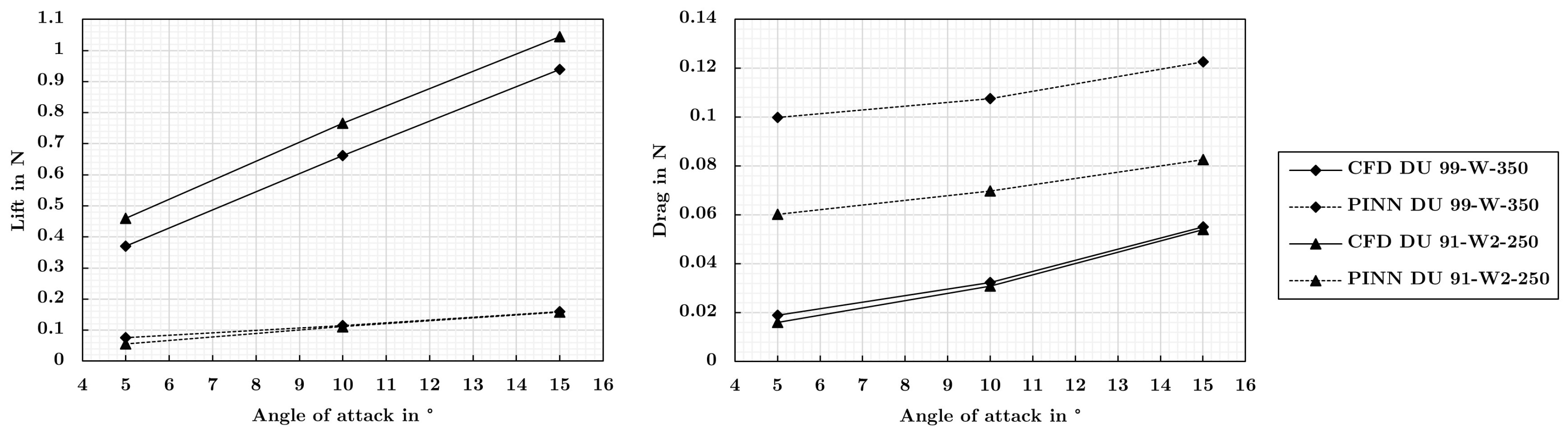
The prediction biases as well as the effects of the AoA where also visible for the lift and drag results. Figure 8 exhibits the lift and drag results of the PINNs in comparison with the reference data. As seen, the networks correctly captured an increase of lift and drag with the AoA. Moreover, the PINNs succesfully captured a higher drag induced by the thicker DU 99-W-350 airfoil. However, the lift was underestimated and the drag was systematically overestimated. The underestimation of the lift is in agreement with the underestimated pressure peaks on the suction surface of both airfoils, visible in Figure 6 and Figure 7.
4. Discussion
The results of this study showed that the mixed-variable networks were capable to serve as qualitative surrogate models to predict the Reynolds-averaged flow fields developing with the AoA. The networks captured the essential flow features, lift and drag values increasing with the AoA, and recognized a higher drag of the thicker airfoil. However, there were significant quantitative deviations from the reference CFD simulations as the extremes of the velocity and pressure fields were underestimated and the shear layer thicknesses were overestimated. At this precision, the results could not compete with traditional CFD calculations.
Sun et al. [29] conducted a similar study of a surrogate model also trained in an unsupervised manner on the flow around an airfoil under variable AoA and reported very good agreements with the reference solution. However, the Reynolds number of the problem was on the order of and, hence, very low. In our study, we investigated flows at a Reynolds number on the order of . This results in a more complicated optimization problem as the shear layers become much thinner and, consequently, the gradients of the solution field become much steeper, the nonlinear convection terms begin to dominate the RANS equations, and a turbulence model needs to be included that also adds to the complexity of the system of equations. As reported by Harmening et al. [12], a surrogate model of the DU 99 W-350 airfoil featuring very good agreement with the reference data could be obtained when incorporating labeled data into the training routine. In fact, a majority of studies concerning elevated Reynolds numbers applied PINNs while incorporating labeled data [5,7,11,12,15,22,23,34,35].
Rao et al. [3] reported a superior performance of a mixed-variable network trained in an unsupervised manner on a laminar flow when compared with a traditional PINN. This finding was confirmed by Harmening et al. [8], who reported a significantly increased performance for Reynolds-averaged flows around cylinders. However, as evident by the findings of the present study as well as of [8], there are further methodological improvements necessary when applying physics-informed deep learning to flows at high Reynolds numbers without training data.
The deviations between the predictions and the reference solutions were due to turbulence modeling deviations, training or optimization errors, and approximation errors. While the turbulence modeling differences could be eliminated by applying two equation turbulence models such as the k- model, these were reported to be subject to stability issues during the training when applied with or without labeled training data [8,12]. In fact, to the best knowledge of the authors, the only so far reported successful applications of turbulence models to unsupervised physics-informed deep learning were using the mixing length model [8,10]. Hence, development of a method to successfully apply two equation turbulence models to physics-informed deep learning is a question for future research. To reduce the training error, more sophisticated deep learning methods are required. Krishnapriyan et al. [17] investigated failure modes of PINNs and reported improved results by using curriculum learning. Other studies that focused improvements of PINN methods to tackle complex problems also applied adaptive loss weighting and Fourier feature networks [33]. Besides, convolutional or U-Net PINNs [16,21,30,32,36], and distributed PINNs [4], among others, could potentially yield improved predictions.
The investigated unsupervised physics-informed deep learning method showed to be capable to qualitatively capture the flow fields and the underlying physics. Hence, the remaining improvements are of quantitative nature. It is not clear if any of the above suggested enhanced methods or any other method would bridge the remaining gap. However, as only quantitative and no more fundamental changes to the predictions are required, to our eyes, further methodological work is worthwhile. Many PINN studies focused on laminar flows at low Reynolds numbers. In contrast, the present work is aimed to motivate methodological studies focused on Reynolds-averaged flows at elevated Reynolds numbers due to the technical significance of such flows and the usefulness of corresponding surrogate models which could make great use in the investigation and design of aerodynamic systems.
In fact, surrogate models based on physics-informed deep learning would feature several traits that make them favorable when compared to traditional simulations. Firstly, no computational grid needs to be constructed to train a PINN as the training points can be sampled randomly within the domain. Secondly, the solution field is not subject to errors caused by a discretization scheme as the deviations of the RANS equations can be obtained directly via backpropagation. Most importantly, as shown by [2,10,28,29,30,29] and also visible from the results of the present work, PINNs could be used to solve several solution fields, corresponding to several settings of a parameter, simultaneously in a single training instance. Furthermore, the trained PINNs can later be used to give a prediction for arbitrary settings of said parameter. This is a fundamental advantage over traditional simulations that can only be used to solve a single solution field in a single computational process. To obtain a solution for a parameter setting not solved yet, a model would need to be fitted in a second step to several independent solutions. However, as discussed above, further improvements of the physics-informed deep learning method are necessary to obtain high fidelity PINN-based surrogate models.
5. Summary and Conclusions
In the present work, we explored the capabilities and limitations of mixed-variable networks to serve as surrogate models of 2.5-dimensional flow fields around two airfoils under variable angles of attack. The models were trained to solve the Reynolds-averaged Navier-Stokes equations incorporating Prandtl’s mixing length model depending on the angle of attack. The main findings are summarized as follows:
- Using the investigated method, it was possible to train a single network to learn the family of flow fields corresponding to variable angles of attack between 5° and 15° without generation of a computational grid. This is a substantial advantage over traditional solvers that could only by used to calculate a single solution field for a single angle of attack at a time. After successful improvement of the method, this trait would make physics-informed deep learning a powerful tool for surrogate modeling.
- The models captured qualitative features of the high Reynolds number flow fields such as high gradient boundary layers, stagnation regions, and wakes. Furthermore, the models recognized lift and drag values increasing with the angle of attack and the higher drag of the thicker airfoil. It is remarkable that all of these features were predicted without incorporating labeled reference data into the training routine.
- However, compared to the reference simulations, the extremes of the velocity and pressure fields were underestimated and the thicknesses of the shear layers were overestimated by the PINNs. Consequently, the lift was underestimated and the drag was overestimated for both airfoils. With the observed performance, PINNs can not currently compete with traditional computations in terms of accuracy. The difficulty of the deep learning problem and the resulting limited accuracy of the predictions is a consequence of the elevated Reynolds number of the problem. More work is necessary to further develop the PINN-based surrogate method.
- Future studies should focus on successfully implementing two equation turbulence models and reducing the training error by applying more advanced training methods. The present study is aimed to outline the potential capabilities of simultaneous unsupervised physics-informed deep learning and to encourage further research and methodological developments of the technique under application to high Reynolds number flows.
Author Contributions
J.H.H.: Conceptualization; Investigation; Methodology; Software; Project administration; Writing – original draft. F.J.P.: Resources; Supervision; Writing – review and editing. O.el M.: Supervision; Writing – review and editing.
Data Availability Statement
The data that support the findings of this study are available from the corresponding authors upon request.
Conflicts of Interest
The authors have no conflicts to disclose.
References
- E. H. W. Ang, G. Wang, and B. F. Ng. Physics-informed neural networks for low reynolds number flows over cylinder. Energies, 16(12), 2023. [CrossRef]
- C. J. Arthurs and A. P. King. Active training of physics-informed neural networks to aggregate and interpolate parametric solutions to the navier-stokes equations. Journal of Computational Physics, 438:None, 2021. [CrossRef]
- C. Rao, H. Sun, and Y. Liu. Physics-informed deep learning for incompressible laminar flows. Theoretical and Applied Mechanics Letters, 10(3):207–212, 2020. [CrossRef]
- V. Dwivedi, N. Parashar, and B. Srinivasan. Distributed physics informed neural network for data-efficient solution to partial differential equations, 2019. Preprint at http://arxiv.org/pdf/1907.08967v1.
- H. Eivazi, M. Tahani, P. Schlatter, and R. Vinuesa. Physics-informed neural networks for solving reynolds-averaged navier–stokes equations. Physics of Fluids, 34(7):075117, 2022. [CrossRef]
- M. Fernández-Delgado, M. S. Sirsat, E. Cernadas, S. Alawadi, S. Barro, and M. Febrero-Bande. An extensive experimental survey of regression methods. Neural networks : the official journal of the International Neural Network Society, 111:11–34, 2019. [CrossRef]
- S. Ghosh, A. Chakraborty, G. O. Brikis, and B. Dey. Rans-pinn based simulation surrogates for predicting turbulent flows. 2023. Preprint at https://arxiv.org/pdf/2306.06034.pdf.
- J. H. Harmening, F.-J. Peitzmann, and O. el Moctar. Effect of network architecture on physics-informed deep learning of the reynolds-averaged turbulent flow field around cylinders without training data. Frontiers in Physics, 12, 2024. [CrossRef]
- J. H. Harmening, F. Pioch, and D. Schramm. Physics informed neural networks as multidimensional surrogate models of cfd simulations. In Machine Learning und Artificial Intelligence in Strömungsmechanik und Strukturanalyse, Wiesbaden, Germany, 16.–17. may, pages 71–80. NAFEMS, may 2022.
- O. Hennigh, S. Narasimhan, M. A. Nabian, A. Subramaniam, K. Tangsali, Z. Fang, M. Rietmann, W. Byeon, and S. Choudhry. Nvidia simnet™: An ai-accelerated multi-physics simulation framework. In M. Paszynski, D. Kranzlmüller, V. V. Krzhizhanovskaya, J. J. Dongarra, and P. M. Sloot, editors, Computational Science – ICCS 2021, volume 12746 of Lecture Notes in Computer Science, pages 447–461. Springer International Publishing, Cham, 2021.
- W. Huang, X. Zhang, W. Zhou, and Y. Liu. Learning time-averaged turbulent flow field of jet in crossflow from limited observations using physics-informed neural networks. Physics of Fluids, 35(2), 2023. [CrossRef]
- J. H. Harmening, F. Pioch, L. Fuhrig, F.-J. Peitzmann, D. Schramm, and O. el Moctar. Data-assisted training of a physics-informed neural network to predict the reynolds-averaged turbulent flow field around a stalled airfoil under variable angles of attack. 2023. Preprint at https://www.preprints.org/manuscript/202304.1244/v1.
- X. Jin, S. Cai, H. Li, and G. E. Karniadakis. Nsfnets (navier-stokes flow nets): Physics-informed neural networks for the incompressible navier-stokes equations. Journal of Computational Physics, 426:109951, 2021. [CrossRef]
- J. Jonkman, S. Butterfield, W. Musial, and G. Scott. Definition of a 5-mw reference wind turbine for offshore system development, 2009.
- V. Kag, K. Seshasayanan, and V. Gopinath. Physics-informed data based neural networks for two-dimensional turbulence. Physics of Fluids, 34(5), 2022. [CrossRef]
- Y. Kim, Y. Choi, D. Widemann, and T. Zohdi. A fast and accurate physics-informed neural network reduced order model with shallow masked autoencoder. Journal of Computational Physics, 451:110841, 2022. [CrossRef]
- A. Krishnapriyan, A. Gholami, S. Zhe, R. Kirby, and M. W. Mahoney. Characterizing possible failure modes in physics-informed neural networks. In M. Ranzato, A. Beygelzimer, Y. Dauphin, P.S. Liang, and J. Wortman Vaughan, editors, Advances in Neural Information Processing Systems, volume 34, pages 26548–26560. Curran Associates, Inc, 2021.
- I. E. Lagaris, A. Likas, and D. I. Fotiadis. Artificial neural networks for solving ordinary and partial differential equations. IEEE transactions on neural networks, 9(5):987–1000, 1998. [CrossRef]
- R. Laubscher and P. Rousseau. Application of a mixed variable physics-informed neural network to solve the incompressible steady-state and transient mass, momentum, and energy conservation equations for flow over in-line heated tubes. Applied Soft Computing, 114:108050, 2022. [CrossRef]
- L. Lu, X. Meng, Z. Mao, and G. E. Karniadakis. Deepxde: A deep learning library for solving differential equations. SIAM Review, 63(1):208–228, 2021. [CrossRef]
- H. Ma, Y. Zhang, N. Thuerey, X. H. null, and O. J. Haidn. Physics-driven learning of the steady navier-stokes equations using deep convolutional neural networks. Communications in Computational Physics, 32(3):715–736, June 2022. [CrossRef]
- Y. Patel, V. Mons, O. Marquet, and G. Rigas. Turbulence model augmented physics informed neural networks for mean flow reconstruction, 2023. Preprint at http://arxiv.org/pdf/2306.01065v1.
- F. Pioch, J. H. Harmening, A. M. Müller, F.-J. Peitzmann, D. Schramm, and O. el Moctar. Turbulence modeling for physics-informed neural networks: Comparison of different rans models for the backward-facing step flow. Fluids, 8(2):43, 2023. [CrossRef]
- M. Raissi, P. Perdikaris, and G. E. Karniadakis. Physics informed deep learning (part i): Data-driven solutions of nonlinear partial differential equations, 2017. Preprint at http://arxiv.org/pdf/1711.10561v1.
- M. Raissi, P. Perdikaris, and G. E. Karniadakis. Physics informed deep learning (part ii): Data-driven discovery of nonlinear partial differential equations, 2017. Preprint at http://arxiv.org/pdf/1711.10566v1.
- M. Raissi, P. Perdikaris, and G. E. Karniadakis. Physics-informed neural networks: A deep learning framework for solving forward and inverse problems involving nonlinear partial differential equations. Journal of Computational Physics, 378:686–707, 2019. [CrossRef]
- M. Raissi, A. Yazdani, and G. E. Karniadakis. Hidden fluid mechanics: Learning velocity and pressure fields from flow visualizations. Science (New York, N.Y.), 367(6481):1026–1030, 2020. [CrossRef]
- L. Sun, H. Gao, S. Pan, and J.-X. Wang. Surrogate modeling for fluid flows based on physics-constrained deep learning without simulation data. Computer Methods in Applied Mechanics and Engineering, 361:112732, 2020. [CrossRef]
- Y. Sun, U. Sengupta, and M. Juniper. Physics-informed deep learning for simultaneous surrogate modeling and pde-constrained optimization of an airfoil geometry. Computer Methods in Applied Mechanics and Engineering, 411:116042, 2023. [CrossRef]
- N. Wandel, M. Weinmann, and R. Klein. Teaching the incompressible navier-stokes equations to fast neural surrogate models in 3d. Physics of Fluids, 33(4):047117, 2021. [CrossRef]
- H. Wang, Y. Liu, and S. Wang. Dense velocity reconstruction from particle image velocimetry/particle tracking velocimetry using a physics-informed neural network. Physics of Fluids, 34(1):017116, 2022. [CrossRef]
- R. Wang, K. Kashinath, M. Mustafa, A. Albert, and R. Yu. Towards physics-informed deep learning for turbulent flow prediction. In R. Gupta, Y. Liu, M. Shah, S. Rajan, J. Tang, and B. A. Prakash, editors, Proceedings of the 26th ACM SIGKDD International Conference on Knowledge Discovery & Data Mining, pages 1457–1466, New York, NY, USA, 08232020. ACM.
- S. Wang, S. Sankaran, H. Wang, and P. Perdikaris. An expert’s guide to training physics-informed neural networks, 2023. Preprint at https://arxiv.org/pdf/2308.08468.pdf.
- M.-J. Xiao, T.-C. Yu, Y.-S. Zhang, and H. Yong. Physics-informed neural networks for the reynolds-averaged navier–stokes modeling of rayleigh–taylor turbulent mixing. Computers & Fluids, 266:106025, 2023.
- H. Xu, W. Zhang, and Y. Wang. Explore missing flow dynamics by physics-informed deep learning: The parameterized governing systems. Physics of Fluids, 33(9):095116, 2021. [CrossRef]
- Y. Zhu, N. Zabaras, P.-S. Koutsourelakis, and P. Perdikaris. Physics-constrained deep learning for high-dimensional surrogate modeling and uncertainty quantification without labeled data. Journal of Computational Physics, 394(1):56–81, 2019. [CrossRef]
Figure 1.
Geometry of the DU 99-W-350 airfoil featuring variable angles of attack inside the channel.
Figure 1.
Geometry of the DU 99-W-350 airfoil featuring variable angles of attack inside the channel.
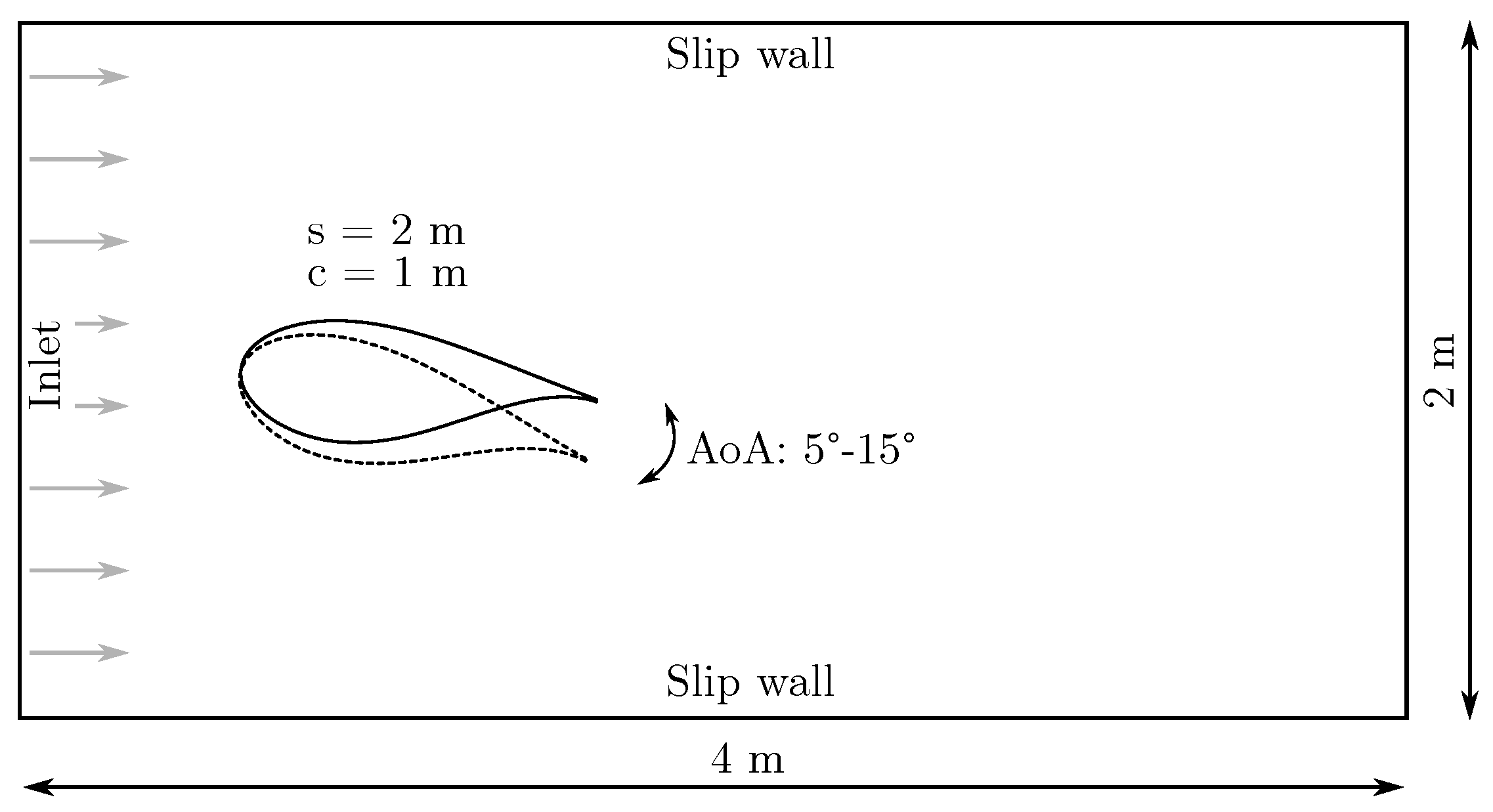
Figure 2.
Velocity fields around the DU 99-W-350 airfoil for different angles of attack as predicted by the PINN in comparison with the reference simulations.
Figure 2.
Velocity fields around the DU 99-W-350 airfoil for different angles of attack as predicted by the PINN in comparison with the reference simulations.
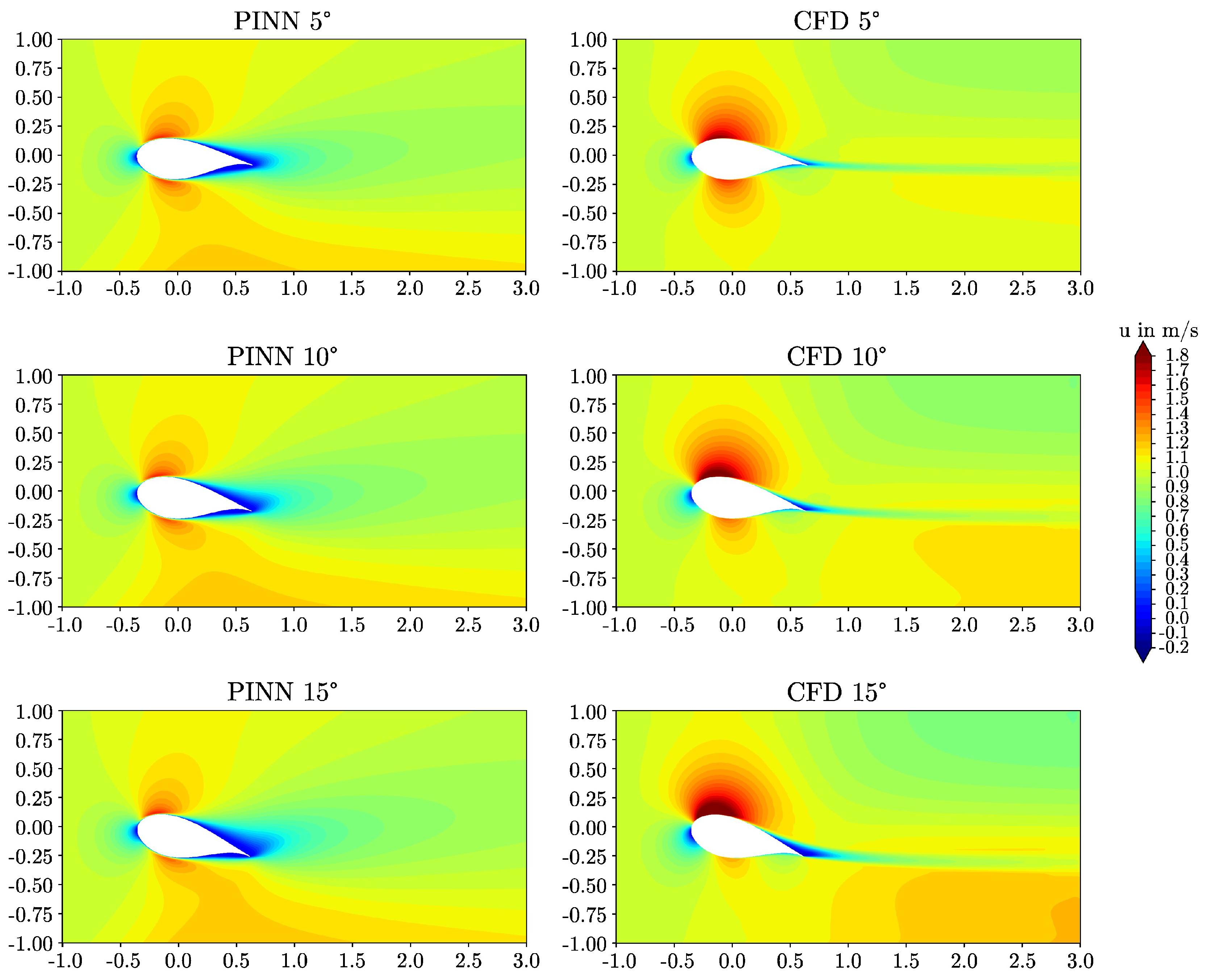
Figure 3.
Boundary layer on the suction surface of the DU 99-W-350 airfoil as predicted by the PINN in comparison with the reference simulation. Left: Boundary layer at an angle of attack of 5° at . Right: Boundary layer at an angle of attack of 15° at .
Figure 3.
Boundary layer on the suction surface of the DU 99-W-350 airfoil as predicted by the PINN in comparison with the reference simulation. Left: Boundary layer at an angle of attack of 5° at . Right: Boundary layer at an angle of attack of 15° at .
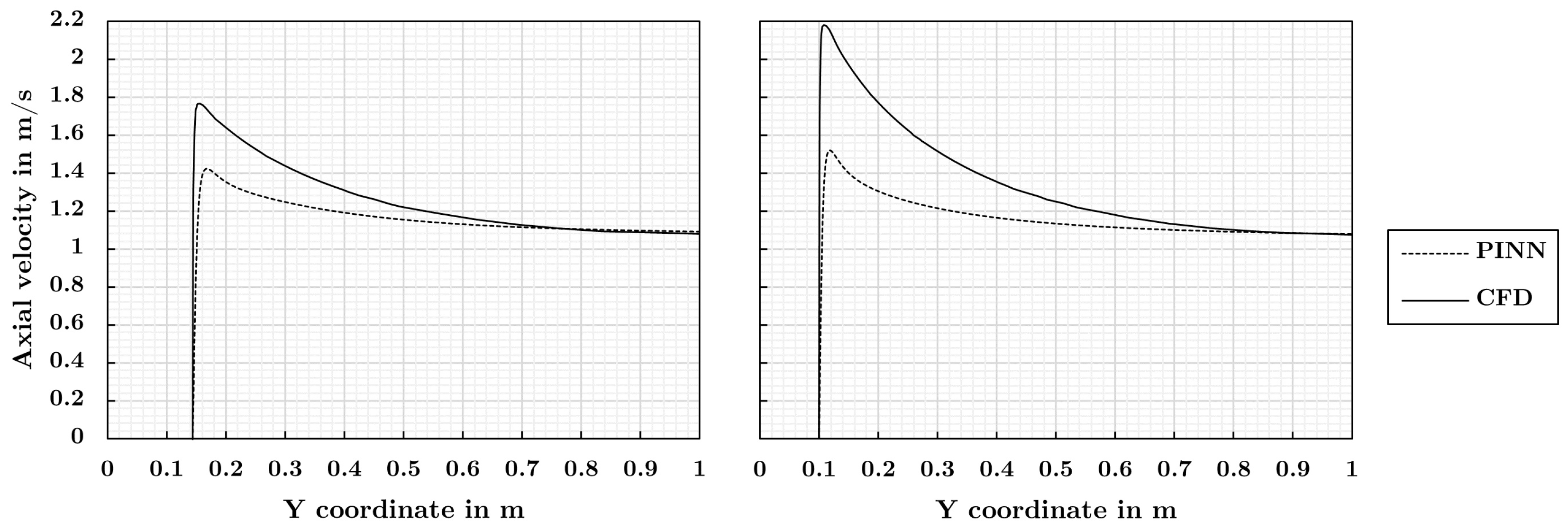
Figure 4.
Velocity fields around the DU 91-W2-250 airfoil for different angles of attack as predicted by the PINN in comparison with the reference simulations.
Figure 4.
Velocity fields around the DU 91-W2-250 airfoil for different angles of attack as predicted by the PINN in comparison with the reference simulations.
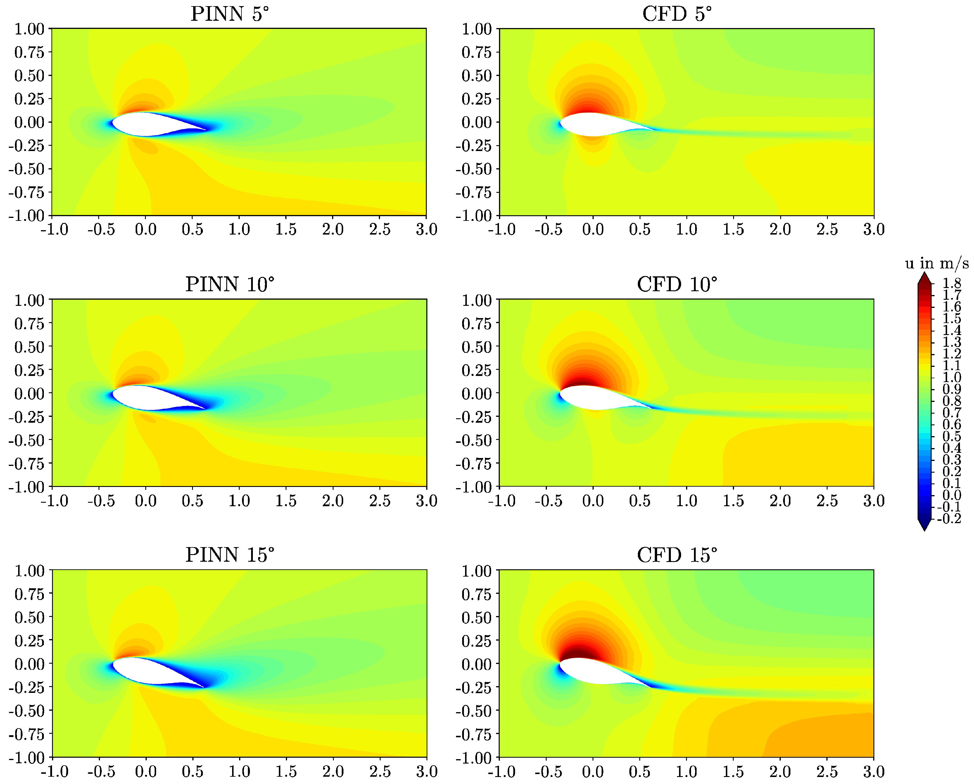
Figure 5.
Boundary layer on the suction surface of the DU 91-W2-250 airfoil as predicted by the PINN in comparison with the reference simulation. Left: Boundary layer at an angle of attack of 5° at . Right: Boundary layer at an angle of attack of 15° at .
Figure 5.
Boundary layer on the suction surface of the DU 91-W2-250 airfoil as predicted by the PINN in comparison with the reference simulation. Left: Boundary layer at an angle of attack of 5° at . Right: Boundary layer at an angle of attack of 15° at .
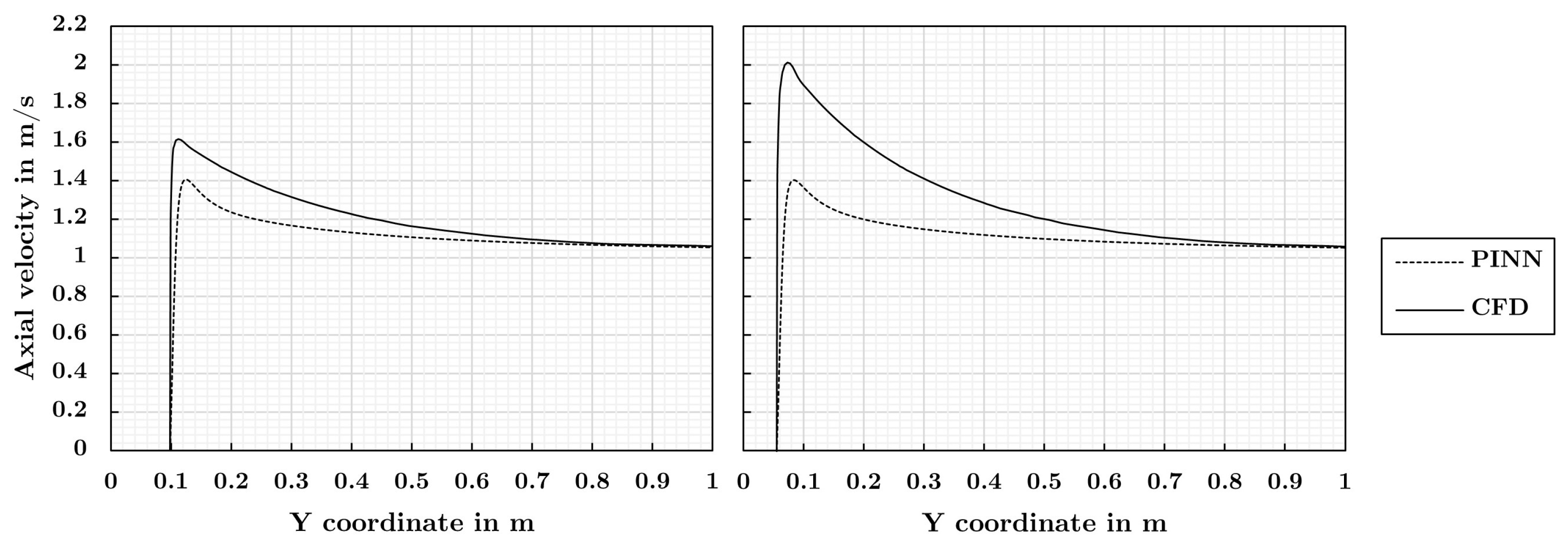
Figure 6.
Pressure fields around the DU 99-W-350 airfoil for different angles of attack as predicted by the PINN in comparison with the reference simulations.
Figure 6.
Pressure fields around the DU 99-W-350 airfoil for different angles of attack as predicted by the PINN in comparison with the reference simulations.
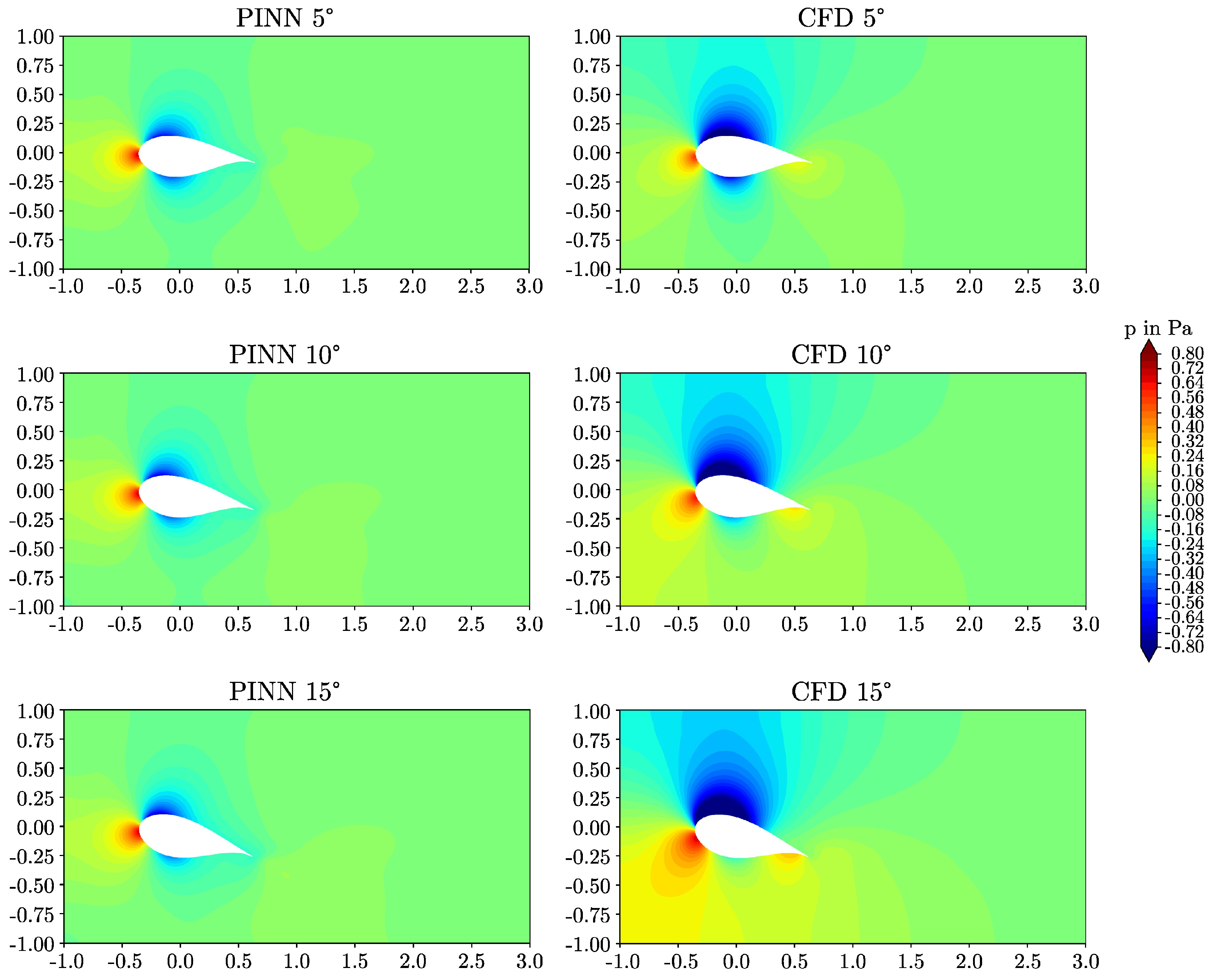
Figure 7.
Pressure fields around the DU 91-W2-250 airfoil for different angles of attack as predicted by the PINN in comparison with the reference simulations.
Figure 7.
Pressure fields around the DU 91-W2-250 airfoil for different angles of attack as predicted by the PINN in comparison with the reference simulations.
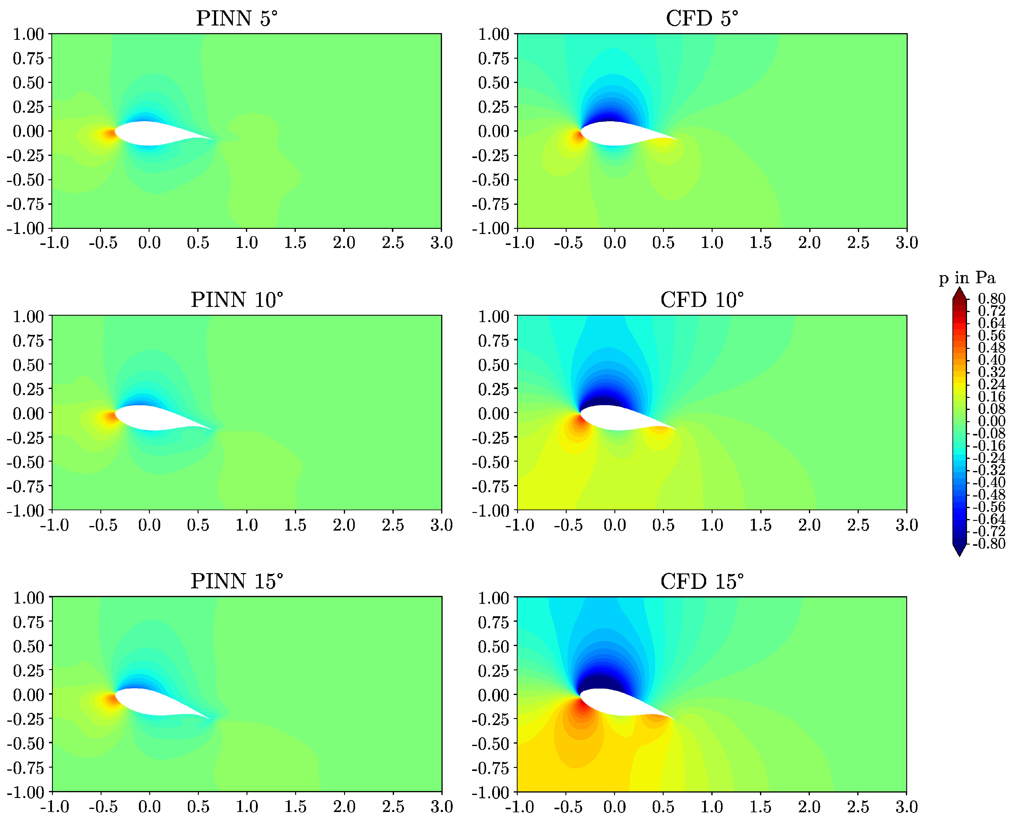
Figure 8.
Lift and drag results for both airfoils as predicted by the PINNs in comparison with the reference data. Left: Lift. Right: Drag.
Figure 8.
Lift and drag results for both airfoils as predicted by the PINNs in comparison with the reference data. Left: Lift. Right: Drag.
Disclaimer/Publisher’s Note: The statements, opinions and data contained in all publications are solely those of the individual author(s) and contributor(s) and not of MDPI and/or the editor(s). MDPI and/or the editor(s) disclaim responsibility for any injury to people or property resulting from any ideas, methods, instructions or products referred to in the content. |
© 2024 by the authors. Licensee MDPI, Basel, Switzerland. This article is an open access article distributed under the terms and conditions of the Creative Commons Attribution (CC BY) license (http://creativecommons.org/licenses/by/4.0/).
Copyright: This open access article is published under a Creative Commons CC BY 4.0 license, which permit the free download, distribution, and reuse, provided that the author and preprint are cited in any reuse.


