
Submitted:
16 June 2025
Posted:
17 June 2025
You are already at the latest version
Abstract
Designing gas turbine combustors that operate effectively with turbomachinery components over a wide range of operating conditions is a challenging task, requiring detailed 3D computational fluid dynamics (CFD) analysis, which is computationally intensive. To alleviate this, surrogate models of the different sub-components like the pre-diffuser, combustion zone, dilution zone and transition ducting can be employed. These component-level models can then be integrated with surrogate models of turbomachinery components to enable comprehensive whole-engine multi-point optimization. This paper presents the development of a data-driven surrogate model for conical air pre-diffusers that can be utilized to perform design optimization, what-if analysis, and be integrated within larger system-level simulation models. The surrogate model is developed within the spectral graph convolution neural network (GCN) framework to predict the 2D symmetry plane velocity, temperature and pressure distributions. The model is trained on CFD simulation data encompassing diffusers with diverse geometric parameters, including a wide range of aspect ratios, diffuser lengths, and inlet diameters, as well as various combinations of boundary conditions. As input, the surrogate model receives graphs representing the symmetry plane meshes, along with vectorized boundary condition values for each training sample. Different layer architectures are investigated to share information between the GCN and fully connected layers that process the graph and boundary condition data respectively. The best-performing surrogate model achieves high predictive accuracy, with normalized mean absolute percentage errors below 1% for pressure and temperature, and below 3.9% for velocity.
Keywords:
deep learning
; graph convolutional networks
; conical diffusers
; computational fluid dynamics
1. Introduction
Optimization of combustors is one of the more challenging aspects of gas turbine design [1]. Successful combustor designs should ensure high combustion efficiency, low pollutant emissions and adequate lean blowout and extinction margins. These design requirements often conflict with one another, making development and optimization of combustors operating over a wide range particularly difficult [2]. Moreover, the high computational expense of 3D combustion computational fluid dynamics (CFD) simulations further prohibits effective design and optimization across multiple operating conditions. Multi-fidelity surrogate modelling of gas turbine combustor components has been demonstrated to be an effective approach to enable timely optimization of combustors [3]. These data-driven surrogate models can be trained on CFD simulation results, experimental data [2], reactor network simulation results [1] or analytical model results. A particularly exciting strategy involves developing separate surrogate models of varying complexities for individual combustor components such as the pre-diffuser, combustion zone, dilution zone and transition ducting. These component-level models can then be integrated with surrogate models of turbomachinery components [4], enabling truly comprehensive whole-engine multi-point optimization across a wide range of operating conditions.
Within gas turbine combustors, pre-diffusers play an essential role in combustion performance by efficiently decelerating compressor discharge flow to appropriate velocities without incurring any unnecessary entropy generation. As compressor discharge velocities increase and combustor design requirements grow more challenging, the performance of the pre-diffuser becomes increasingly critical to overall system efficiency [5]. The present work presents a data-driven surrogate modelling approach for conical pre-diffusers, which can be utilized to perform design optimization, what-if analysis, and be integrated within larger system-level simulation models. The spectral graph convolution neural network framework [6], which processes graph data, is utilized along with CFD simulation results to develop the surrogate model. This geometric deep learning framework maps input graph node features, such as spatial coordinates, along with non-graph data, such as boundary conditions, to corresponding flow field variables at the graph nodes. Furthermore, this geometric deep learning framework can train on multiple graphs (which represents different diffuser geometries), allowing it to process and learn the effects of both geometric variations and varying boundary conditions on resultant flow field variables [7]. This capability enables accurate prediction of detailed flow fields within unparameterized diffuser geometries, as opposed to traditional deep learning surrogate models which are limited to predicting flow fields only for specific geometric representations on which they were trained [8,9].
Over recent years many researchers have investigated the use of deep learning to develop surrogate models of expensive 2D and 3D CFD simulations with a range of applications such as virtual sensors [10], control system optimization [11], design space exploration for computationally efficient design optimization [12], and as part of multi-fidelity simulations (e.g., turbulence closure surrogate model within larger simulations [13]). These CFD-based surrogate models can be applied to a range of tasks, from basic predictions of global 0D post-processed results, such as area-weighted temperatures, to more complex reconstructions of 2D or 3D flow and temperature fields. Models with higher target dimensionality are computationally more expensive to train, require greater network capacity, and face increased risk of overfitting, thereby demanding substantially larger training datasets. For these reasons, many researchers have adopted sophisticated deep learning architectures, such as convolutional neural networks, when developing these CFD-based surrogate models. Herewith follows a short overview of selected recent publications.
Wu et al. [9] developed surrogate models capable of predicting the flow fields around 2D aerofoils. The authors developed an integrated architecture combining a convolutional neural network with a generative adversarial network (GAN), establishing an accurate one-to-one mapping between aerodynamic parameters defining the geometry and the corresponding two-dimensional pressure distribution around the aerofoil. To circumvent the need for large amounts of CFD simulation data to train these deep learning models, Wang et al. [14] proposed a semi-supervised learning approach called discriminative regression fitters (DRF). The proposed approach reduces dataset size requirements by 70% while maintaining prediction accuracy comparable to fully supervised methods. The DRF utilizes the memory property of neural networks and employs a Gaussian mixture model (GMM) to dynamically classify pseudo-labelled data and then minimize the loss by updating the easy and difficult-to-train labelled entries. The approach was successfully demonstrated for 2D aerofoil predictions.
Vandewiel et al. [15] developed a specialized spatial attention UNet-based surrogate model to predict 2D CFD simulated velocity data for flow around a small building based on wind direction, speed and building opening size. The researchers generated approximately 1000 training samples using 3D RANS simulations. Once trained the spatial attention UNet surrogate model achieved a mean absolute percentage error (MAPE) of 4.7% for the velocity predictions, which is a 10% increase in performance compared to the standard attention UNet architecture. To address the challenge of varying geometries, the authors fed 2D pixelated signed distance function representations of the building fluid volumes into the surrogate as inputs along with the boundary conditions. Wu et al. [16], develop a high-fidelity transient surrogate model of turbulent hydrogen combustion in a fixed geometry combustor. The surrogate model employs an encoder-decoder architecture with convolutional layers and noise injection, enabling it to forecast the evolution of combustion reactants, products, and gas temperatures throughout the simulated 2D domain. The researchers compared the accuracy of their proposed deep learning architecture against both UNet and Fourier neural operator models. The results indicated that the proposed model substantially outperforms the standard models.
The work discussed above, like most CFD-based surrogate modelling research, was limited in two ways: it either developed models for fixed geometries or required geometry-aware parametric approaches (such as polynomial representations of aerofoil pressure and suction side profiles). To overcome these geometric constraints when developing surrogate models capable of outputting 2D or 3D flow fields, geometric deep learning can be utilized. It directly processes the spatial structure of the domain as graphs, which enable these models to be geometry agnostic [7]. Recent studies have highlighted the advantages of applying geometric deep learning to the development of CFD-based surrogate models. Gouttiere et al. [7], developed a surrogate model capable of predicting the flow and pressure field through the NASA rotor 37 axial compressor stage using CFD simulation data and geodesic convolutional neural networks (GCNNs). The surrogate model uses graphs created from STL file data of the blade, hub, shroud and circumferential pitch average surfaces as inputs along with the scalar valued boundary conditions such as velocity inlet and pressure outlet values. Each graph node contains specific spatial coordinates, and the surrogate model generates predictions for flow field and pressure values at these precise nodal locations along with global performance values such as total-to-total pressure ratio across the compressor stage. Once trained the GCNN model could predict various global performance values such as isentropic efficiency and pressure ratio within 1% accuracy compared to the ground truth CFD simulation data. Leveraging the shape-independent nature of their GCNN modelling approach, the researchers applied the surrogate model to perform local geometric shape optimizations. Through these optimizations, they demonstrated a significant 3.25% increase in isentropic efficiency by modifying the three-dimensional blade geometry.
Mallya et al. [17], similar to the previous study of Gouttiere et al., developed a GCNN surrogate model using CFD simulation data. The surrogate model was developed to predict the 3D velocity, pressure and temperature fields for the flow through structured and unstructured porous volumes of different shapes. As inputs the surrogate model receives the graphs representing the volumetric and surface meshes along with global parameters such as total surface area and porosity of the porous volume. The surrogate model consisted of parallel GCNN and fully connected (FC) layers with residual skip connections. The initial layers of the architecture shared information by using mean pooling as a mechanism to combine the GCNN layer outputs with the FC layer outputs. The authors, similar to Gouttiere et al. [7], did not specify exactly how the sharing of data signals is achieved between the GCNN and FC layers, and therefore this sharing of data signals will be investigated in the current work. The Mallya et al. model achieved high prediction accuracies for temperature and heat flux fields (90% and 70% respectively). However, the velocity field predictions were considerably less accurate, with average accuracy values as low as 14% for the various cases analysed. The model demonstrated superior accuracy in predicting global performance metrics, such as overall pressure drop and melt time, when compared to a conventional multilayer perceptron (MLP) network. This performance advantage highlights the GCNN’s capacity to effectively disentangle complex spatial relationships in the data.
Feng et al. [18], used graph convolutional networks (GCNs) to develop a surrogate model capable of predicting the 2D temperature field for the natural convection flow around heated cylinders in a cylindrical container. The simulation data was generated for 400 different heated cylinder arrangements and surface temperature combinations using the opensource CFD package OpenFOAM. The researchers compared the trained GCN surrogate model accuracy with that of MLP- and convolutional network-based surrogate models. The GCN surrogate model produced results with MAPEs in the order of 0.1% and showed approximately 85% improvements compared to the predictions by the MLP and convolutional network surrogate models.
In the present work, a GCN surrogate model is developed capable of predicting the 2D symmetry plane velocity, temperature and pressure distributions for flows within conical air diffusers. The model is trained on CFD simulation data encompassing diffusers with diverse geometric parameters, including a wide range of aspect ratios, diffuser lengths, and inlet diameters. Additionally, the training incorporates various boundary condition combinations. As input the surrogate model receives the graphs representing the symmetry plane meshes (coordinates and corresponding cell volumes) along with vectorized boundary condition values for a given training sample. This work investigates different layer architectures used to share information between the GCN and fully connected (FC) layers processing the graph and boundary condition data respectively. Additionally, the study examines the effects of hyperparameters such as batch sizes, number of layers, number of neurons per layer and spatial graph densities on prediction accuracy. Graph densities are varied by increasing edge connectivity, allowing nodes to connect with a greater number of surrounding nodes. To the best of the authors’ knowledge, this is the first research that sets out to develop a geometric deep learning surrogate model for air flow within a conical diffuser. Furthermore, the work investigates unique layer architectures which will be shown to produce sufficiently accurate velocity, temperature and pressure predictions for a wide range of diffuser geometries and boundary conditions. The computer models developed in the present work used Python 3.12.7, PyTorch 2.7.0, PyTorch Geometric 2.7.0, scikit-learn 1.6 and SciPy 1.15.2.
2. Materials and Methods
Figure 1 shows the overview of the proposed GCN-based surrogate model used to predict the velocity, pressure and temperature fields within the conical air diffusers. The inputs to the surrogate model are batches of graphs and boundary conditions, where the boundary values are assumed to be uniform across the relevant inlet or outlet boundary plane. The graph batches consist of multiple graphs where each graph is a representation of a specific diffuser geometry. A graph consists of node features and edges. The node features are the x- and y-coordinates and cell volumes, and the edges are connections between the nodes. Cell volumes are included as input node features to help the model distinguish between small boundary layer cells and larger free stream cells. In this work, CFD mesh coordinates and volumes serve as node features, with connectivity determined using the K-Nearest Neighbour (KNN) algorithm, which identifies the K nearest cells and establishes connections accordingly. While Delaunay triangulation represents a more direct adjacency matrix construction method, the KNN approach is employed for its ability to regulate graph density via the neighbourhood parameter selection. Boundary condition batches consist of vectors of boundary condition values, forming matrices where rows correspond to batch samples and columns represent boundary condition features. These two datasets (graph batches and boundary condition batches) are processed through shared network layers, utilizing both FC and GCN layers that allow data to flow between boundary conditions and graph representations. The graph signal then proceeds through GCN layers before producing the final predicted velocity, pressure, and temperature distributions. Both input and output datasets undergo pre-processing and normalization, as discussed later in this section. For instance, the predicted outputs are scaled by subtracting boundary condition values and then normalized using a min-max scaler, thus, creating more appropriately scaled outputs that facilitate efficient training.
This section details the CFD-based data generation methodology, including the simulation parameters, data preprocessing techniques, and theoretical foundations of GCN and FC layers. Finally, the various shared layer architectures evaluated in the surrogate modelling framework will be discussed.
2.1. Parameterised Diffuser Geometry and CFD Model Setup
The air diffuser CFD simulations are performed using the ANSYS Fluent 2024 R2 software. A pipeline that automates geometry generation, grid generation and subsequent simulation is configured using the ANSYS Workbench interface. Figure 2 below shows the geometry with dimensions along with the mesh with boundary conditions indicated. In the figure (left), [m] is the inlet radius of the diffuser, [m] the outlet radius, [m] the inlet length, [m] the outlet length and [m] the diffuser length. The diffuser aspect ratio is defined as and by varying and an entire envelope of diffuser geometries can be defined within the ranges specified for the three geometrical parameters. These three parameters are parameterized in ANSYS and systematically varied to create multiple geometries, which are then used to generate a simulation database for surrogate model training. In the present work, only a ¼ of the diffuser geometry is simulated in 3D, to reduce computational costs across multiple simulations. The diffuser geometry consists of an inlet, outlet, wall and two symmetry patches. The surrogate model, which will be discussed in subsequent sections, predicts velocity, temperature, and pressure distributions along one symmetry patch. While this approach effectively generates results for a 2D axially symmetric plane, 3D CFD simulations were conducted to lay the groundwork for future research where the surrogate model will be expanded to predict complete 3D domain results.
Figure 2 (right) below also shows an example of a generated mesh. To ensure the boundary layer region is properly resolved, five inflation layers with the smooth transition approach is applied to each of the generated meshes. Additionally, to ensure consistent mesh scaling across all geometries, body sizing with element dimensions set at is implemented to ensure a qualitatively well-structured mesh. The present study specifically examines the capability of GCN model architectures to predict CFD-simulated fields, not to develop highly accurate mesh and simulation solutions. Consequently, mesh generation is simplified relative to real-world simulation practices.
To simulate the steady-state turbulent flows within the diffuser geometries the Reynolds-averaged Navier-Stokes formulations of the relevant transport equations are utilized. As some of the generated simulation samples could have Mach numbers exceeding a value of 0.3, compressible effects had to be considered. Therefore, the Coupled pressure-based solver is utilized and the density of the fluid is resolved using the ideal gas equation of state. The steady-state mass, momentum and energy balance equations solved by the CFD code are shown in equations (1), (2) and (3) respectively.
In the above equations, is the spatial dimension in direction , [m/s] the directional velocity, [Pa] the fluid static pressure, [J/kg] total energy, [kg/m3] fluid density, [K] fluid temperature, [kg/ms] fluid viscosity and [W/mK] effective fluid conductivity. The fluctuating Reynold stresses are approximated using the Boussinesq equation [19] as shown in equation (4) where the turbulent viscosity is in turn calculated as . The turbulent viscosity is also used to calculated the effective thermal conductivity where [W/mK] is the fluid thermal conductivity and [J/kgK] the fluid specific heat. The fluid properties such as and are calculated using the built-in values within Fluent 2024 R2.
To close the Boussinesq equation, the turbulent kinetic energy [m2/s2] and turbulent kinetic energy dissipation rate [m2/s3] are solved using the realizable turbulence model which is often used for combustor CFD simulations [20]. To account for the wall effects on the turbulent flow the standard wall function is applied in the near-wall regions. For the simulations, the pressure term is discretized using the PRESTO! scheme and the momentum and energy equations are discretized using the second-order upwind scheme. The turbulent kinetic energy and dissipation rate are discretized using the first-order upwind scheme. Simulation convergence is determined based on reduction of scaled residual values below 1e-3 for continuity, 1e-4 for the velocity equations and 1e-6 for the energy equation. Simulations that do not meet these criteria during the database generation phase are automatically rejected and excluded from the final simulation database.
The inlet of the diffuser (see Figure 2) is set as a uniform velocity inlet type boundary condition with the uniform inlet temperature specified. The outlet of the domain is set to a uniform pressure outlet condition with the backflow temperature set to the temperature inlet value. The walls are specified as standard no-slip walls and the symmetry planes as symmetry boundary conditions. The inlet velocity [m/s], outlet pressure [Pa] and inlet temperature [K] are parameterised and also varied along with the geometrical parameters in Figure 2 to create the simulation database for surrogate model training.
2.2. Data Generation and Preparation
As previously mentioned, the objective of the current work is to develop a surrogate model using geometric deep learning which predicts the 2D velocity, static pressure and static temperature fields on the symmetry plane of a conical diffuser. The inputs to the surrogate model are: a graph representing the diffuser symmetry plane topology and the accompanying boundary conditions. To train and test the surrogate model, a dataset of CFD simulation meshes and results are generated. These meshes, which were converted into graphs, and the associated flow field results are generated using the CFD methodology combined with a design of experiments (DOE) approach. The DOE approach systematically varied both geometrical parameters and boundary conditions to create a structured simulation matrix. The ranges for each parameter ( and ) are specified and the DOE matrix populated using optimal-space filling with a min-max distance design type. A total of converged simulation points are created and a CFD simulation is performed for each one. Simulations were conducted on an 8-core PC with 32GB of RAM, requiring approximately 48 hours of computation time. The ranges for each input parameter are found in Table 1 below and are typical ranges for combustor pre-diffusers taken from [21]. Upon completion of all the simulations, the boundary conditions input dataset (see Figure 1) used for training and testing the surrogate model has dimensions of where the three features are the boundary condition values for and for the individual samples of the DOE matrix. The remaining surrogate model input data extracted from the simulation dataset are the x-, y-coordinates and cell volumes of the symmetry plane for each mesh generated. Therefore, the dimensions of each sample are where the subscript indicates the simulation index, the mesh size of the simulation and the three features the two coordinates and cell volume. The complete mesh input dataset would then be a tensor of where is the graph input dataset tensor consisting of entries with each entry being a matrix of mesh coordinates and volumes. Similarly, the output dataset for the simulation case has a shape of with the output features being the magnitudes of static temperature, static pressure and fluid velocity for each cell. The complete output graph dataset tensor would have the dimensions .
There are large disparities in scale between the output field variables. For example, static pressure values are in the order of Pa, while static temperatures are in the order of K, and fluid velocity magnitudes in the order of m/s. Therefore, scaling is applied to assist the surrogate model during training. This entailed calculating the difference between the predicted field variable and its corresponding boundary condition value for each simulation case. Therefore, for each entry in the dataset the following scaling is applied to the 1000 entries.
Note in equation (5), , and are the three column vectors of the matrix for the simulation case.
To enable the GCN layers to process the dataset, additional edge connectivity matrices had to be defined for each simulation case. Figure 3 below shows how the CFD mesh and graphs are related in the current work. For the example diagram shown below, the graph is constructed by connecting the graph nodes corresponding to mesh cells to the nearest four nodes. The Pytorch Geometric library [22] requires the edge connectivity for a graph to be provided in a compact format as shown in the figure below with two edges used between two graph nodes. The compact connectivity format has a shape of where is the edge connectivity matrix for the simulation case and is the total number of edges for the specific simulation case. The matrices for the different simulation cases are constructed by first generating an adjacency matrix for each case using the KNN algorithm. This algorithm processes the cell x- and y-coordinates while setting a specified number of connections. Next the adjacency matrices are converted to the compact edge connectivity format using the coordinate matrix conversion in SciPy [23].
With the graph input, boundary condition input and output datasets specified, the final pre-processing step implemented is the normalization of the data. In the present work min-max scalers [24] are utilized for all the input and output datasets and across all the simulation cases.
2.3. Fully Connected and Graph Convolutional Neural Networks
The surrogate model uses shared layers consisting of GCN and FC layers as well as standard GCN layers. For a FC layer the output signal is calculated using equation (6) [25].
In equation (6), is the summed signal from the layer, is the output signal from the previous FC layer, is the weight matrix for the layer and the bias vector. For the initial FC layer, with being the minibatch size for the training of the surrogate model. Several of the architectures investigated in this study incorporate residual connections. In these cases, the summed signal can either be directly passed to an activation function, or first combined with the skip connection signal before activation. ReLu [26] activation functions are used throughout the surrogate network models.
GCN models perform convolutions by updating node values and aggregating information from nearby nodes thereby inducing relational inductive bias [25]. Therefore, GCN layers have the capability to process graph data that can represent a number of structures such as non-Euclidean CFD mesh data [27]. The calculated output signal for node in GCN layer is calculated as shown in equation (7) where is the node output signal vector before activation, is a bias term vector, the weight matrix and the aggregation operation for the specific node. Note the capitals used the following equations, indicates the use in the GCN layers, where in equation (6), lower case symbols for weight and biases matrices and vectors indicate use in FC layers.
In the current work the GCN layer configuration by Kipf and Welling [28] is used. For this type of GCN layer the aggregation operation is performed using equation (8). In this equation, denotes a set containing the indices of the neighbours of the node and the set for the node.
In vectorized form for the entire graph, the Kipf and Welling GCN layer output (before activation) is calculated using equation (9). In the equation below, is the summed signal output for all the nodes in layer , is the previous GCN layer output for all the nodes, is the adjacency matrix for the specific graph and is the diagonal degree matrix. For the GCN layers used in the present work, self-loops were not included.
Similar to the FC layers, GCN layers are implemented both with and without residual connections in the tested architectures. In configurations with skip connections, the summed output signal from a GCN layer is combined with the residual connection signal before being passed through the ReLU activation function creating the layer output signal . When residual connections are absent, the summed signal proceeds directly to the ReLU activation. Equation (9) is formulated for an single graph (corresponding to a single CFD simulation case in this work). However, as with FC layer calculations, mini-batching is desirable to reduce the computational burden during surrogate model training. To achieve this, PyTorch Geometric employs a solution wherein adjacency matrices are stacked diagonally (constructing a comprehensive graph containing multiple disconnected subgraphs), while node and target features are concatenated along the nodal dimension. Therefore, no changes were made to the GCN layers to enable mini-batching in the present work.
At the final GCN layer of the surrogate model, numbered , the calculated output matrix is set equal to the target matrix for the simulation case, in other words . To ensure that the surrogate model correctly maps the input graph and boundary condition data to the correct output target data, the network parameters for the FC and GCN layers namely , , and for each layer should be optimized to minimize the selected cost function . The selected cost function is the mean squared error (MSE) loss, which is calculated for the simulation case as shown in equation (10).
In equation (10), is the node target vector dimension (columns corresponding to velocity, pressure and temperature predictions), is the predicted node target feature at node and feature and is the actual node target values. The previous equation represents the loss function for a single graph. The overall loss function is the average of these individual losses across all training and testing cases as shown in equation (11).
To adjust the network weights and biases to minimize the selected cost function, the Adam optimization algorithm [29] is used. The Adam algorithm is shown below in equation (12) for the trainable network parameter . At the start of the training phase, the scaling () and momentum () matrices are initialized to 0. The parameter tracks iteration count, while (set to 0.9) controls momentum decay and (set to 0.999) governs scaling decay. The learning rate parameter is initially set to 0.001. An exponential learning rate decay is implemented, which adjusts the learning rate value ten times throughout the training process using the relation where is the decay rate parameter which is set to a value of 0.9.
2.4. Network Architecture Designs and Training
Multiple deep learning architectures were evaluated to determine the optimal configuration for the surrogate model. These architectures incorporate upsampling, residual connections, concatenation of layer signals, layer normalization and pooling. Most of these operations are only implemented for the shared layers where the FC and GCN layer outputs share information. Figure 4 illustrates the various shared and GCN layer architectures implemented. In the following discussion the signals propagating from boundary condition inputs into FC layers are designated as scalar data signals, while those traversing into GCN layers are classified as graph input data signals.
For architecture 1 (A1) the GCN and FC layers have the same amount of neurons, therefore, for a single graph the output dimensions for the two layers would be (signal G) and respectively, where is the number of neurons for layer . After passing the layer outputs through ReLu activation functions they are combined by applying node-based mean pooling to the GCN output resulting in signal P which has the same dimensions as the FC layer output. These two signal are then summed together creating signal S. After summation the signal S is then upsampled by mapping the summed features to each node in the graph (creating signal U) and adding this to the original GCN layer output (signal G) creating the input for the next GCN layer. The summed vector signal S is the input for the next FC layer. For architecture 2 (A2), rather than pooling the signal G down to the FC layer output dimensionality, the latter is upsampled and added to signal G. Signal S is then pooled down to the original FC layer output dimensionality. Architecture 3 (A3) is similar to A1, but rather than adding signal U to signal G, a concatenation operation is performed, thereby maintaining the original signal G more rigorously compared to previous architectures. This operation generates signal C in the shared layer. Architecture 4 (A4) has the same structure as A2 with the summation of signal G and U being replaced by a concatenation operation. The difference between architectures 5 & 7 (A5 & A7) is that for A5 there is no layer normalization applied. A5 is similar to A3 with the addition of skip connection signals Z and Q being added to the GCN and FC layer outputs respectively. As demonstrated in the subsequent results, the summation variant was not evaluated since the concatenation operation consistently yielded superior performance. Architectures 6 & 8 (A6 & A8) are similar to the A2 with the addition of residual connections. Again, the difference between A6 and A8 is that A6 does not have layer normalization applied the FC and GCN layer outputs. For the A1-A4 standard GCN layers are used with ReLu activation functions. For A5-A8 residual connections are used throughout the GCN layers.
The considered architectures for the shared layer blocks are described below, with reference to Figure 4. For all architectures, the GCN and FC layers have the number of neurons. Therefore, for a single graph, the output dimensions for the two layers would be and respectively, where is the number of neurons for layer
The developed geometric deep learning surrogate model has various hyperparameters such as layer architecture (Figure 4), number of layers, number of neurons per layer, mini-batch size and graph densities. In this study, a sequential tuning methodology is implemented, beginning with coarse grid search evaluations for each parameter setting. The best-performing configuration from each stage is then retained when tuning subsequent parameters, creating a sequential tuning process. For all steps in the sequential tuning process, the train-test data split is set to 90% training data and 10% testing data.
The first part of the hyperparameter tuning process evaluates the various architectures previously discussed using 256 neurons per hidden layer, 2 shared layers, 3 GCN layers, number of node connections set to 4, and mini-batch size of 8. These models are all trained for 1000 epochs. The best-performing architecture from this initial phase is subsequently retrained with varying network configurations, including different quantities of shared and GCN layers, and different hidden layer dimensions of 64, 128, 256, and 512 neurons. In these subsequent investigations, the training epochs were extended to 2000.
The two models demonstrating the lowest testing errors were then selected to investigate mini-batch size effects. Mini-batch sizes of 1, 4, 8, 16 and 32 were considered. Finally, using the optimal model from the mini-batch investigation, graph density effects were evaluated by varying the number of connections per node in the mesh data graph construction. This evaluation tested nodal connection values of 4, 8, and 16.
In addition to the MSE metric, the normalized mean absolute percentage errors (NMAPE) are used to evaluate surrogate model performance for the velocity magnitude, static pressure and static temperature field predictions. The NMAPE is essentially the mean absolute error between the actual and predicted values normalized using the specific boundary condition for the case. Therefore, the NMAPE for field variable (which can be velocity, pressure or temperature) for case can be estimated using equation (13). In the below equation, is the predicted field variable at the specified node and specific case and the actual value.
3. Results and Discussion
3.1. Performance of Different Network Architectures
Table 2 presents the training and testing MSE and NMAPE values obtained during the first phase of architecture evaluation. It is seen that for all evaluated architectures, the pressure and temperature training and testing NMAPEs are below 1%, indicating good predictive performance by the surrogate models. The highest NMAPEs are observed for the velocity predictions; therefore, the current discussions will pertain to the velocity NMAPEs and the MSE values only.
Comparing architectures A1 and A2, the results demonstrate that A2 achieved a 51% lower relative MSE value on the training dataset compared to A1. However, A1 exhibited superior generalization, with a testing MSE 21% lower than A2. Interesting changes in error metrics are observed when substituting the summation operation with concatenation (viz. A3 and A4). For A3 the relative training and testing MSEs are 56% and 31% lower compared to A1, whereas for A4 it is increased by 16% and 6% respectively compared to A2. For these architectures, the models (A1 and A3) that maintain a dedicated processing pathway for scalar data signals (originating from FC layers) tend to perform better during testing compared to models where scalar outputs are derived from pooling operations on mixed graph and boundary signals only (A2 and A4). The architectures with dedicated pathways for the scalar data appear to better preserve the boundary condition features leading to improved generalization.
Next, residual skip connections are added to A3 and A2 resulting in A5 and A6 respectively. The results show that both the training and testing MSEs are reduced further with the addition of skip connections for both architectures. This highlights the importance of improved information flow through the network. Comparing A5 with A3 shows reductions of 13% and 7% for the training and testing errors respectively. Comparing A6 with A2 yields an increase of 4% in the training MSE, whereas the testing MSE shows a decrease of 24%. Interestingly, the addition of layer normalization to these architectures (A7 and A8) leads to considerable increases in both training and testing MSEs. This is most likely due to standardisation of the output layer feature distributions which attenuates important information content, thus diluting the signal importance.
Figure 5 shows the training and testing MSE histories across epochs. Most noticeable is the erratic MSE signals of A7 and A8, showing the slowest decline in errors. During the initial 200 epochs, A3 has the fastest decline in MSEs of all the models and ultimately achieves the 2nd best performance on testing error. At approximately 200 epochs and beyond, the best performing model on testing MSE is A5. The results thus demonstrate that the addition of skip connections yields favourable reductions in both training and testing MSE metrics (although the magnitude of improvement is marginal for the considered case). This phenomenon likely indicates that the signal preservation benefits obtained by the concatenation process in A3 yields the residual connections of A5 partially redundant. Such findings suggest that the primary constraints on predictive performance may not reside in the signal propagation mechanics addressed by skip connections, but rather in alternative aspects of the model configuration, such as the inherent target function complexity. Nonetheless, the architecture selected for subsequent hyperparameter tuning is the best-performing A5 model.
3.2. Hyperparameter Tuning of Selected Networks
3.2.1. Layer Depth and Neuron Count
Using the selected A5 architecture, various combinations of layer depths and number of neurons per hidden layer are tested, with the results summarised in Table 3. As mentioned, these models are trained for 2000 epochs with the exponential learning rate decay applied every 200 epochs. Generally, the results show that the lowest training and testing MSEs are found for the larger (deeper and wider networks), as indicated by the shading of the table cells. The relative percentage increase going from a combined 5-layer deep 64 neurons per hidden layer model to a 9-layer deep 512 neurons per hidden layer model decreases the training and testing MSEs by 58% and 26% respectively. Analysis reveals a 3.2% relative difference in performance metrics between the model variant with 4 shared layers coupled with 3 GCN layers (512 neurons) and the 4 shared layers with 5 GCN layers (512 neurons) model. Given this marginal discrepancy, both architectures warrant further investigation to determine the relationship between mini-batch sizes during the training process on the MSEs.
3.2.2. Mini-Batch Sizes
Figure 6 shows the training and testing MSE values along with the velocity field prediction NMAPEs for the 7- and 9-layer models trained with the different mini-batch sizes. Training MSE values initially decrease as mini-batch size increases from 1 to 4, then increases again at larger batch sizes. For the 7- and 9-layer models, testing MSEs are progressively reduced as batch sizes decrease from 32 to 1. However, the error reduction becomes minimal when reducing batch sizes from 8 to 1, with no substantial changes observed in this range. For the training velocity prediction NMPAEs the general trend shows that smaller batch sizes are preferable. Similarly, the lowest testing velocity prediction NMAPEs are observed for batch sizes of 1.
Overall, for the 9-layer model, the relative reductions in testing MSE and velocity NMAPE from a mini-batch size of 32 to 1 are 54% and 48% respectively. The fact that the surrogate model prefers online learning over batch learning could be attributed to noise induced high variance gradient updates that help the model escape local minima. Alternatively, it could be that the smaller batch sizes enable the learning of subtle patterns more prominently in the testing dataset. Based on these findings, the best-performing model selected for the next hyperparameter tuning step is the 9-layer model with online learning.
3.2.3. Nodal Connectivity
Table 4 contains the MSE and velocity NMAPE values for the 9-layer model with online learning for different numbers of nodal connections. To generate graphs with increased nodal connections, the connectivity parameter in the KNN algorithm is adjusted to the required value. The results indicate that the increase in more connections based on Euclidean distance does not significantly improve network performance. The best-performing model remains the one with nodal connections set to 4. Future work could look at the potential benefits that could be achieved by using graph attention networks to weight the various connections, thus eliminating unnecessary connections.
One final check that is performed, is to investigate the dependency of the surrogate model accuracy on training dataset size. The best-performing model defined above is retrained using the same testing dataset, but with training dataset sizes of 300, 600 and 900 (used in previous tuning steps). For the training errors, no significant decrease is observed (0.5% going from 300 to 900 training samples). Conversely, a substantial decrease in testing error is found. Increasing the training dataset size from 300 to 600 decreases the MSE value by 39% and increasing the dataset size from 600 to 900 reduces the error by a further 15%. It is, therefore, the opinion of the authors, that further gains can be achieved by increasing the training dataset size for the given problem and DOE ranges used, and by training the model for more epochs.
3.3. Evaluation of Best-Performing Graph Convolutional Networks
Figure 7 shows the actual velocity values for every node in each simulation case against the predicted velocity values for the training (approximately 2.2 million points) and testing data (approximately 250 000 points). Both the training and testing results are shaded by the AR.
The training results reveal that several data points fall outside the 10% error band, specifically those corresponding to high ARs and low velocities. These conditions are interconnected, as high AR geometries typically generate flow separation in the diffuser, creating recirculation regions with low velocities in the diffuser channel. Therefore, the surrogate model appears to generate predictions with higher errors in cases where substantial velocity gradients are present due to flow separation. Similarly for the testing data, the largest errors are observed for low velocities and for cases with high ARs. The plots indicate that while the surrogate model exhibits some prediction limitations, the velocity relative percentage error distribution in Figure 7 (bot) demonstrates good overall performance. For the training dataset, 74% of nodal velocity predictions achieve accuracies exceeding 90%, while for the testing dataset, 69% of the predicted nodal velocities achieve accuracies above 90%.
Figure 8 displays the training and testing error distributions for the nodal pressure and temperature predictions. It is clear from the results that the surrogate model predicts these fields with good accuracy, with nearly all the nodal predictions having predictions accuracies above 99%.
To further demonstrate the surrogate model performance, the actual and predicted contours for velocity magnitude, static pressure and static temperature are plotted in Figure 9. In Figure 9, three cases are selected from the training dataset namely, a) case with the largest AR and shortest diffuser length (DL) combination, b) case closest to the mean AR and DL of the training dataset, and c) case with the smallest AR and longest DL combination.
For case a) the predicted velocity contours accurately reproduce the actual velocity contours. The general distribution of the pressure predictions also aligns well with the actual pressure contours, but minor pressure artefacts are predicted near the diffuser inlet and along the wall of the exit straight section which are not present in the actual data. Similar artefacts are observed for the temperature predictions. These artefacts could potentially be removed using physics-based regularization [27] or adding a smoothness promoting loss function [30].
For case b), which features a geometry closely approximating the mean configuration, the surrogate model can predict the velocity, pressure and temperature fields with good accuracy, as expected. Similarly, for case c), the surrogate model exhibits accurate predictive capabilities. Interestingly, the high frequency spatial artefacts observed in case a) are not present in cases b) and c). Based on these three training dataset cases, the surrogate model delivers both qualitatively and quantitatively accurate predictions of the flow and property fields.
Figure 10, like the previous results, shows the actual and predicted velocity, pressure and temperature fields for three cases taken from the testing dataset. These three cases are selected similarly to the previous results (for example, case a) is selected having the geometry with the largest AR and shortest DL combination in the testing dataset). Like the training dataset results, the surrogate model shows good predictive capabilities and can replicate the actual contours relatively accurately. In case a), velocity measurements showed a 3.62% NMAPE with a maximum error of 24.2%, while temperature and pressure fields demonstrated higher precision (0.052% and 0.042% NMAPEs, with maximum errors of 0.59% and 0.43%, respectively). For case b) the NMAPEs for velocity, temperature and pressure fields are 2.51%, 0.07% and 0.03% respectively, with the maximum normalized percentage errors being 21%, 1.01% and 0.3%. The most accurate predictions appeared in case c), with velocity NMAPE dropping to 1.56% (10.5% maximum error) and exceptionally low temperature and pressure field errors (0.046% and 0.017% NMAPEs; maximum errors of 0.256% and 0.166%). These findings for case c) align with expectations, as the surrogate model demonstrates higher accuracy at lower AR values due to the presence of smaller separation regions, which introduce prediction errors.
4. Conclusions
This study details the development of a geometric deep learning-based surrogate model for predicting flow, pressure and temperature contours within a family of conical diffuser geometries using a combination of GCN and FC layers. The surrogate model can make accurate predictions across a wide range of inlet radii, aspect ratios, lengths, and boundary conditions for velocity, pressure, and temperature. Various shared layer architectures, used to process both graph and scalar data signals, are evaluated. It is found that architectures that enforce dedicated processing pathways for the scalar data signals perform better compared to models that rely solely on pooling operations to create the scalar inputs for subsequent layers. Moreover, the concatenation of scalar and graph data signals improves predictive performance due to the enhanced signal preservation compared to architectures using summation operations.
Sequential hyperparameter tuning is performed using the best-performing surrogate model configuration, which features a combination of residual connections and concatenation operations. The selected surrogate model produced reasonable predictions of the velocity magnitude, static pressure and static temperatures fields along the symmetry planes of the diffusers. The pressure and temperature predictions have NMAPEs below 1%, indicating high accuracy, with velocity predictions showing lower but still acceptable NMAPEs of 3.9%. Studying the individual nodal predictions of the entire testing dataset reveals that the main source of velocity prediction errors occurs for cases with large ARs in regions of low velocities. This most likely indicates the model fails to accurately predict the velocities in the regions of flow separation where abrupt velocity changes occur in the radial direction. Future work will investigate the effect of physics-based regularization to enhance velocity predictions in these regions. Furthermore, examination of the predicted results reveals that the surrogate model occasionally generates minor non-physical artefacts in the pressure and temperature fields. While these artefacts do not significantly impact the overall prediction accuracy, they represent physically unrealistic features in the solution. Therefore, future work will investigate the implementation of smoothness-promoting loss functions, such as Graph Laplacian regularization. Additionally, future work should also investigate the performance benefits when using more advanced graph-based network layers such as GMMs (which includes geodesic edge distances between nodes).
References
- Saboohi, Z.F. Ommi, and M. Akbari, Multi-objective optimization approach toward conceptual design of gas turbine combustor. Applied Thermal Engineering, 2019. 148: p. 1210-1223. [CrossRef]
- Reumschüssel, J.M. J.G.R. von Saldern, B. Ćosić, and C.O. Paschereit, Multi-Objective Experimental Combustor Development Using Surrogate Model-Based Optimization. Journal of Engineering for Gas Turbines and Power, 2023. 146(3). [CrossRef]
- Toal, D.J.J. X. Zhang, A.J. Keane, C.Y. Lee, and M. Zedda, The Potential of a Multifidelity Approach to Gas Turbine Combustor Design Optimization. Journal of Engineering for Gas Turbines and Power, 2021. 143(5). [CrossRef]
- Aulich, M. G. Goinis, and C. Voß Data-Driven AI Model for Turbomachinery Compressor Aerodynamics Enabling Rapid Approximation of 3D Flow Solutions. Aerospace, 2024. 11. [CrossRef]
- Klein, A. , Characteristics of combustor diffusers. Progress in Aerospace Sciences, 1995. 31(3): p. 171-271. [CrossRef]
- Bronstein, M.M. J. Bruna, Y. LeCun, A. Szlam, and P. Vandergheynst, Geometric Deep Learning: Going beyond Euclidean data. IEEE Signal Processing Magazine, 2017. 34(4): p. 18-42. [CrossRef]
- Gouttiere, A. G. Alessi, D. Wunsch, L. Zampieri, and C. Hirsch, Realtime CFD Based Shape Optimization Using Geometric Deep Learning for Families of Turbomachinery Applications. 2023.
- Laubscher, R. and P. Rousseau, An integrated approach to predict scalar fields of a simulated turbulent jet diffusion flame using multiple fully connected variational autoencoders and MLP networks. Applied Soft Computing, 2021. 101: p. 107074. [CrossRef]
- Wu, H. X. Liu, W. An, S. Chen, and H. Lyu, A deep learning approach for efficiently and accurately evaluating the flow field of supercritical airfoils. Computers & Fluids, 2020. 198: p. 104393. [CrossRef]
- Guzmán, C.H. , et al. Implementation of Virtual Sensors for Monitoring Temperature in Greenhouses Using CFD and Control. Sensors, 2019; 19. [Google Scholar] [CrossRef]
- Shi, Y. W. Zhong, X. Chen, A.B. Yu, and J. Li, Combustion optimization of ultra supercritical boiler based on artificial intelligence. Energy, 2019. 170: p. 804-817. [CrossRef]
- Vardhan, H. D. Hyde, U. Timalsina, P. Volgyesi, and J. Sztipanovits, Sample-efficient and surrogate-based design optimization of underwater vehicle hulls. Ocean Engineering, 2024. 311: p. 118777. [CrossRef]
- Kontou, M.G. V.G. Asouti, and K.C. Giannakoglou, DNN surrogates for turbulence closure in CFD-based shape optimization. Applied Soft Computing, 2023. 134: p. 110013. [CrossRef]
- Wang, X. Y. Dong, S. Zou, L. Zhang, and X. Deng, A semi-supervised framework for computational fluid dynamics prediction. Applied Soft Computing, 2024. 154: p. 111422. [CrossRef]
- Vandewiel, M.R. D.D. Eneyew, A.D. Awol, M.A.M. Capretz, and G.T. Bitsuamlak, Approximating CFD simulations of natural ventilation: A deep surrogate model with spatial attention mechanism. Journal of Building Engineering, 2025. 105: p. 112425. [CrossRef]
- Wu, S. H. Wang, and K.H. Luo, A robust autoregressive long-term spatiotemporal forecasting framework for surrogate-based turbulent combustion modeling via deep learning. Energy and AI, 2024. 15: p. 100333. [CrossRef]
- Mallya, N. P. Baqué, P. Yvernay, A. Pozzetti, P. Fua, and S. Haussener, Geodesic Convolutional Neural Network Characterization of Macro-Porous Latent Thermal Energy Storage. ASME Journal of Heat and Mass Transfer, 2023. 145(5). [CrossRef]
- Feng, F. Y.-B. Li, Z.-H. Chen, W.-T. Wu, J.-Z. Peng, and M. Mei, Graph convolution network-based surrogate model for natural convection in annuli. Case Studies in Thermal Engineering, 2024. 57: p. 104330. [CrossRef]
- Versteeg, H.K. , An introduction to computational fluid dynamics the finite volume method, 2/E. 2007: Pearson Education India.
- Fatehi, M. and M. Renzi, Modelling and development of ammonia-air non-premixed low NOX combustor in a micro gas turbine: A CFD analysis. International Journal of Hydrogen Energy, 2024. 88: p. 1-10. [CrossRef]
- Lefebvre, A.H. , Gas turbine combustion. 1 ed. 1983: Hemisphere Publishing Corp.
- Fey, M. and J.E. Lenssen, Fast Graph Representation Learning with PyTorch Geometric. arXiv, 2019.
- Virtanen, P. , et al., SciPy 1.0: fundamental algorithms for scientific computing in Python. Nature Methods, 2020. 17(3): p. 261-272.
- Pedregosa, F. , et al., Scikit-learn: Machine Learning in Python. J. Mach. Learn. Res., 2011. 12(null): p. 2825–2830.
- Prince, S. , Understanding Deep Learning. 2023: MIT Press.
- Nair, V. and G.E. Hinton, Rectified linear units improve restricted boltzmann machines, in Proceedings of the 27th International Conference on International Conference on Machine Learning. 2010, Omnipress: Haifa, Israel. pp. 807–814.
- Peng, J.-Z. N. Aubry, Y.-B. Li, M. Mei, Z.-H. Chen, and W.-T. Wu, Physics-informed graph convolutional neural network for modeling geometry-adaptive steady-state natural convection. International Journal of Heat and Mass Transfer, 2023. 216: p. 124593. [CrossRef]
- Kipf, T.N. and M. Welling, Semi-Supervised Classification with Graph Convolutional Networks. International Conference on Learning Representations (ICLR), 2017.
- Kingma, D.P. and J. Ba, Adam: A Method for Stochastic Optimization. arXiv:1412.6980, 2014.
- Jiang, B. and D. Lin, Graph Laplacian Regularized Graph Convolutional Networks for Semi-supervised Learning. arXiv:1809.09839, 2018.
Figure 1.
Overview of GCN-based surrogate model.
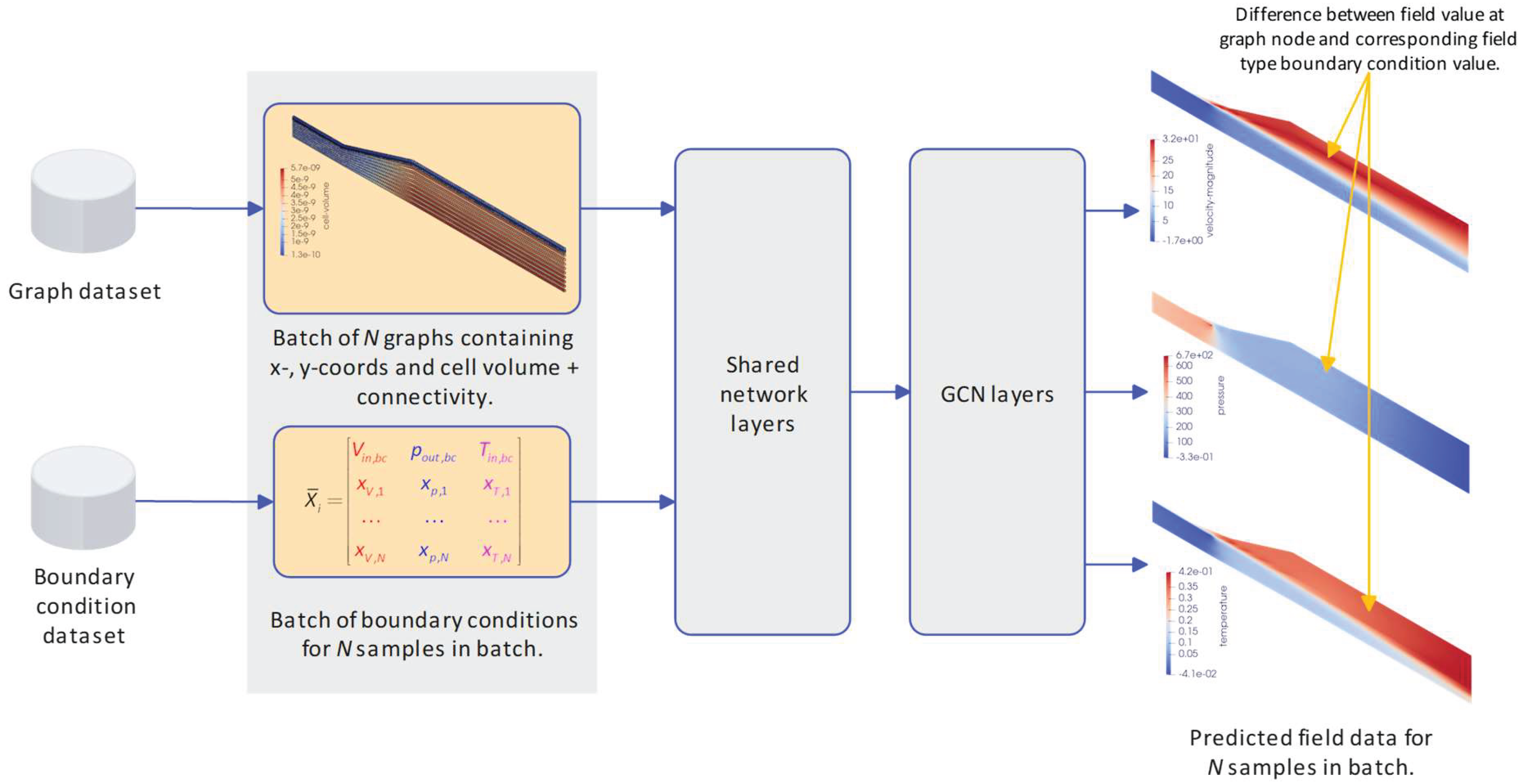
Figure 2.
Geometry and mesh of 1/4 conical diffuser.
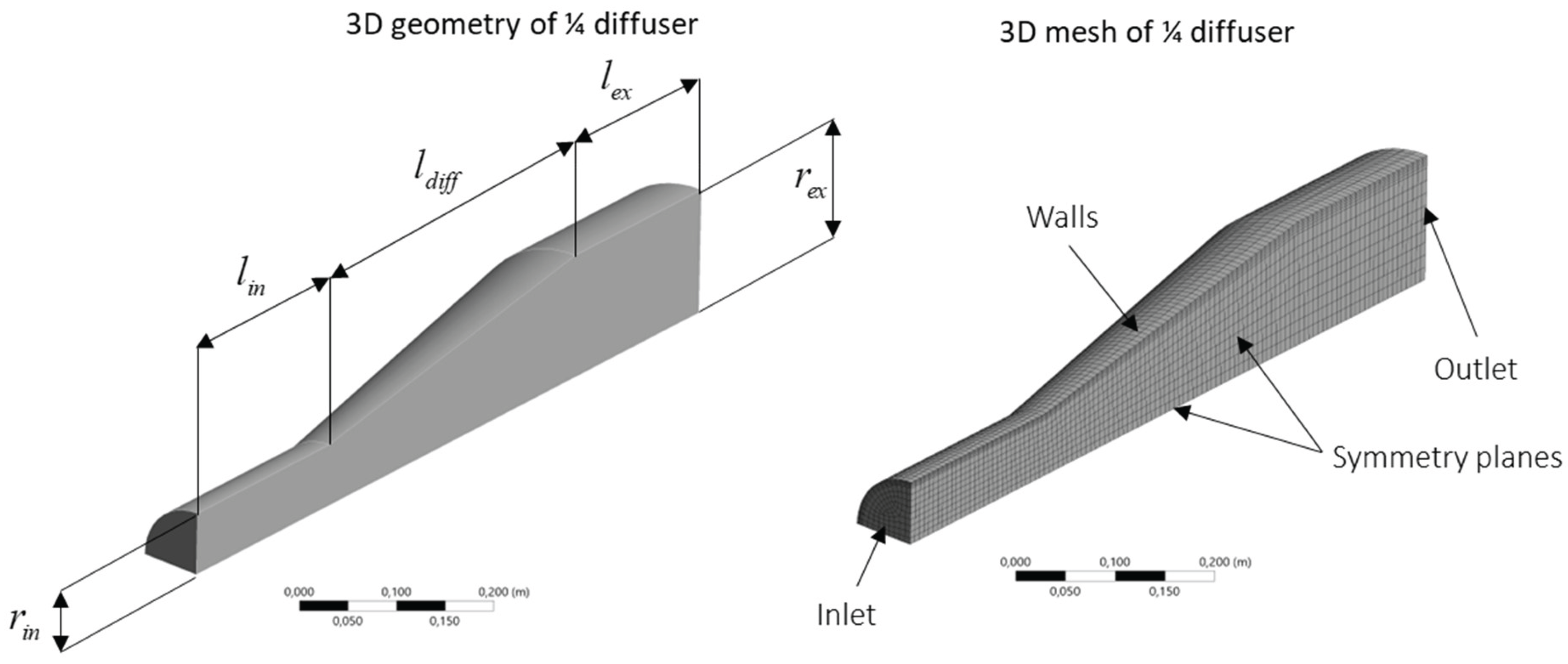
Figure 3.
Mesh to graph conversion.
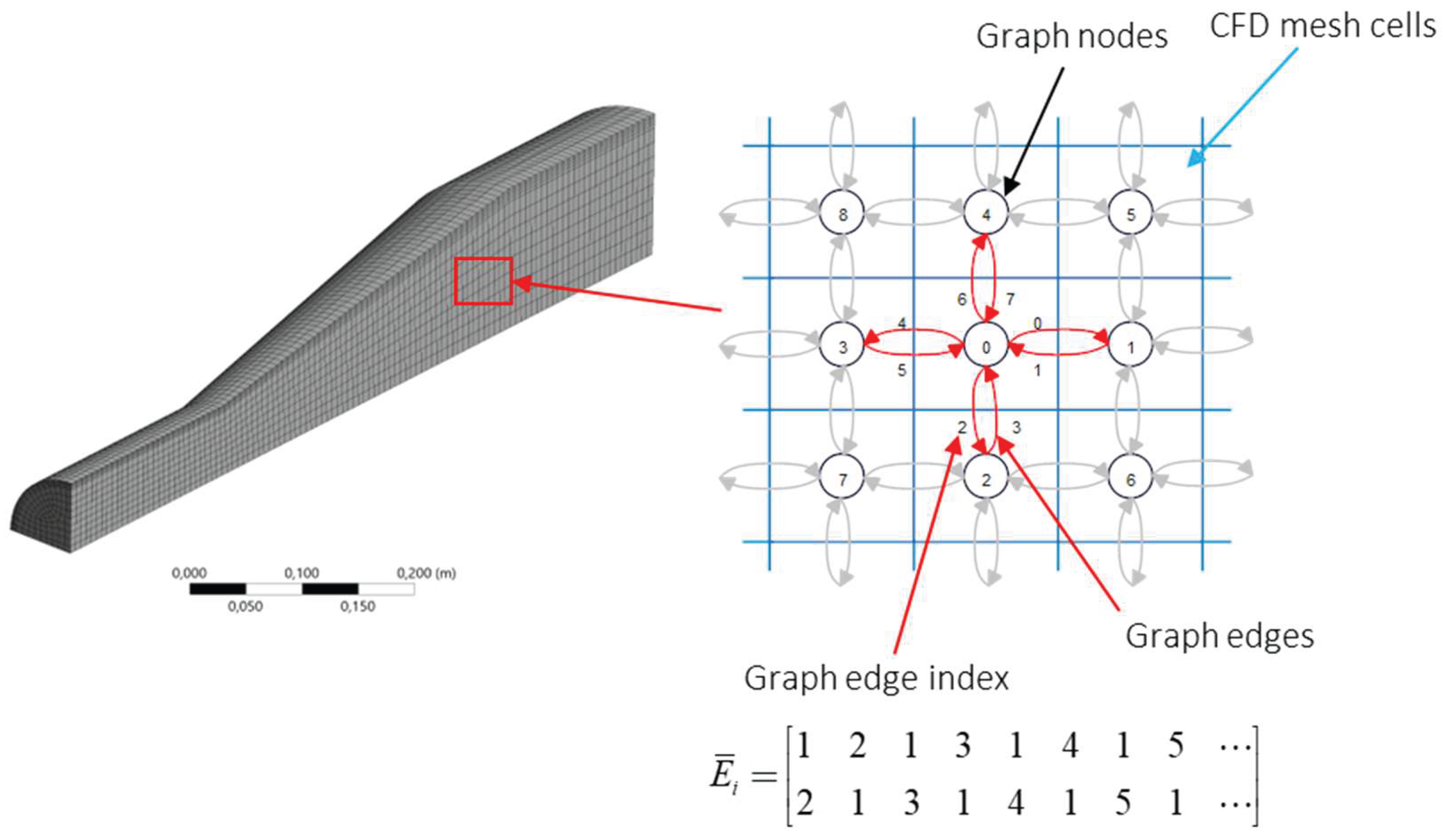
Figure 4.
Tested layer architectures for the surrogate model.
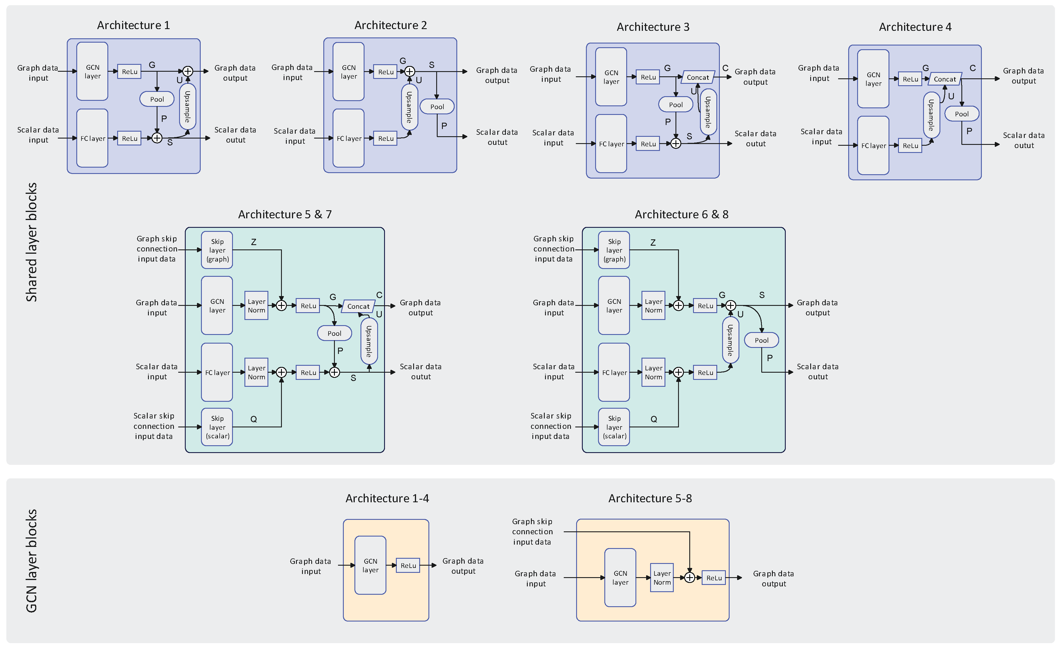
Figure 5.
Training and testing histories as a function of epochs for different architectures.
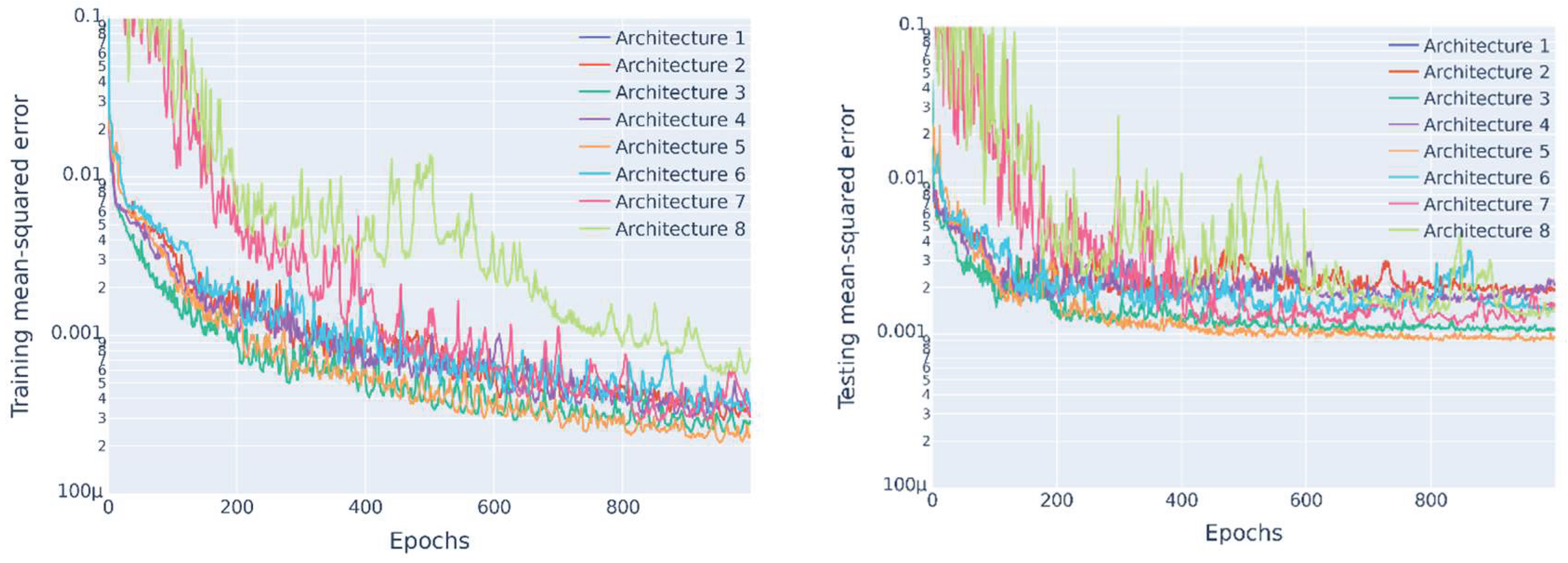
Figure 6.
Training and testing MSEs and NMAPEs obtained for different mini-batch sizes using A5.
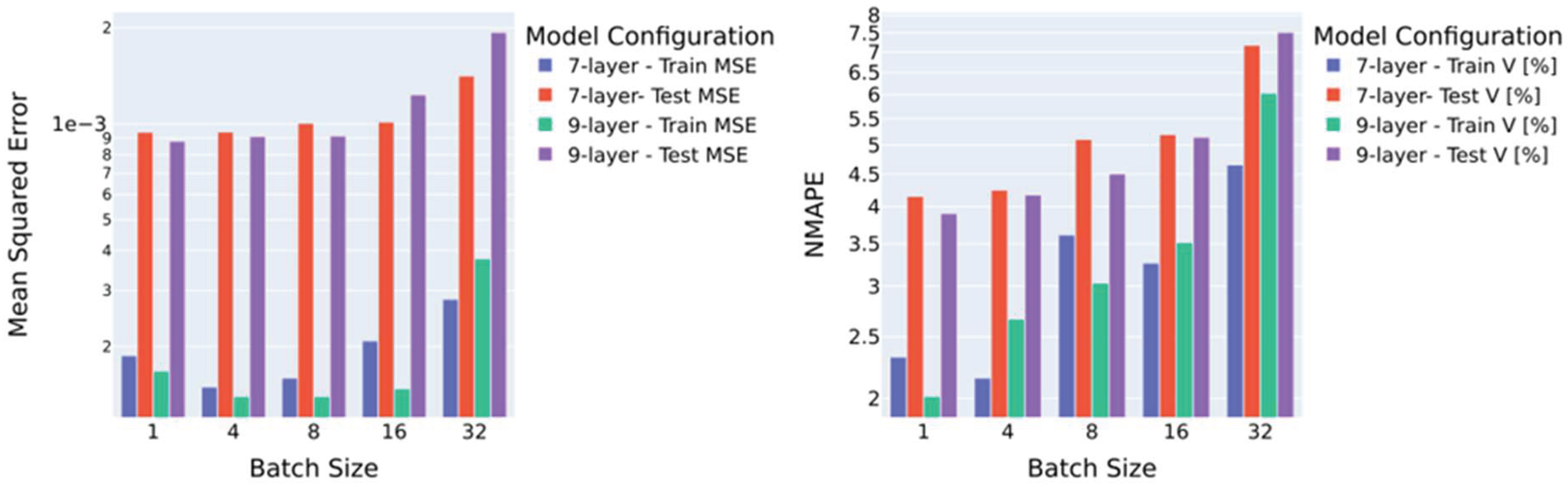
Figure 7.
Actual vs. predicted velocities (training and testing) and velocity prediction error distribution (orange colour in figure is the overlapping region).
Figure 7.
Actual vs. predicted velocities (training and testing) and velocity prediction error distribution (orange colour in figure is the overlapping region).
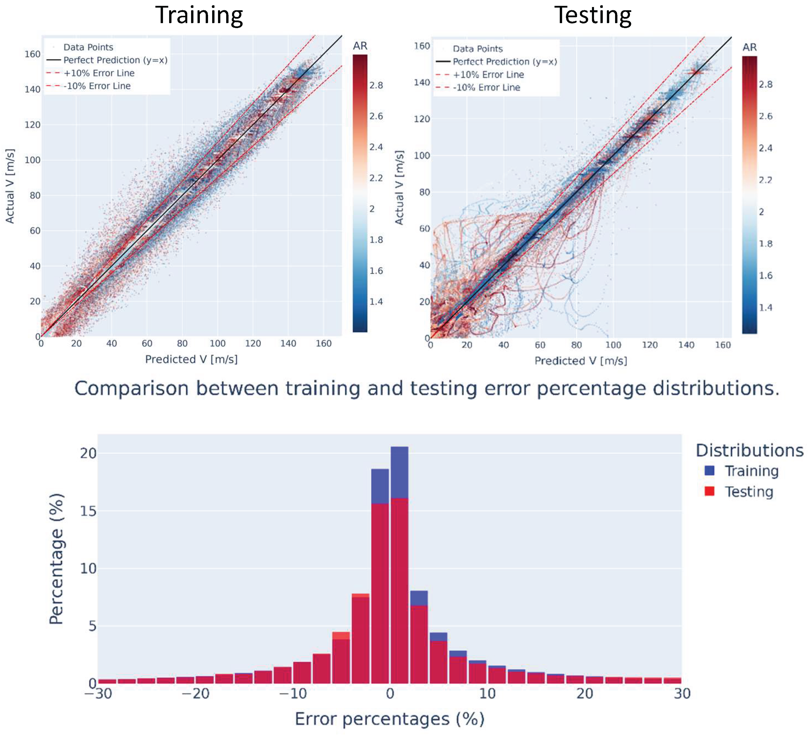
Figure 8.
Training and testing pressure and temperature prediction error distributions.
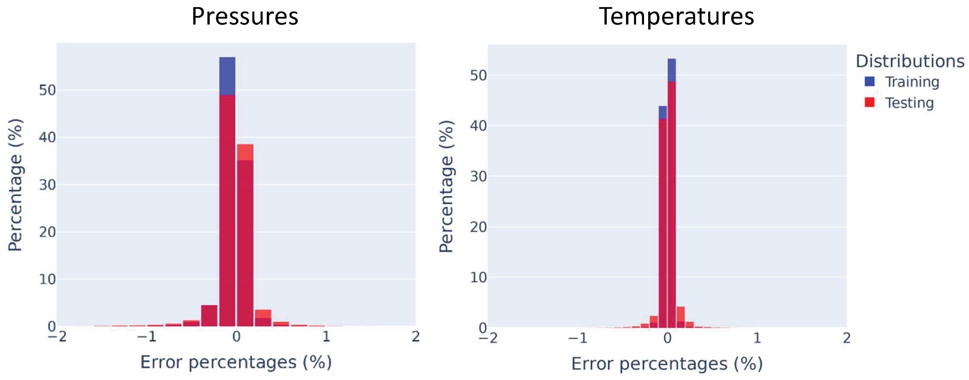
Figure 9.
Actual and predicted contours for training dataset. a) Largest AR with shortest DL case, b) closest to the mean AR and DL of the dataset case and c) smallest AR and largest DL case.
Figure 9.
Actual and predicted contours for training dataset. a) Largest AR with shortest DL case, b) closest to the mean AR and DL of the dataset case and c) smallest AR and largest DL case.
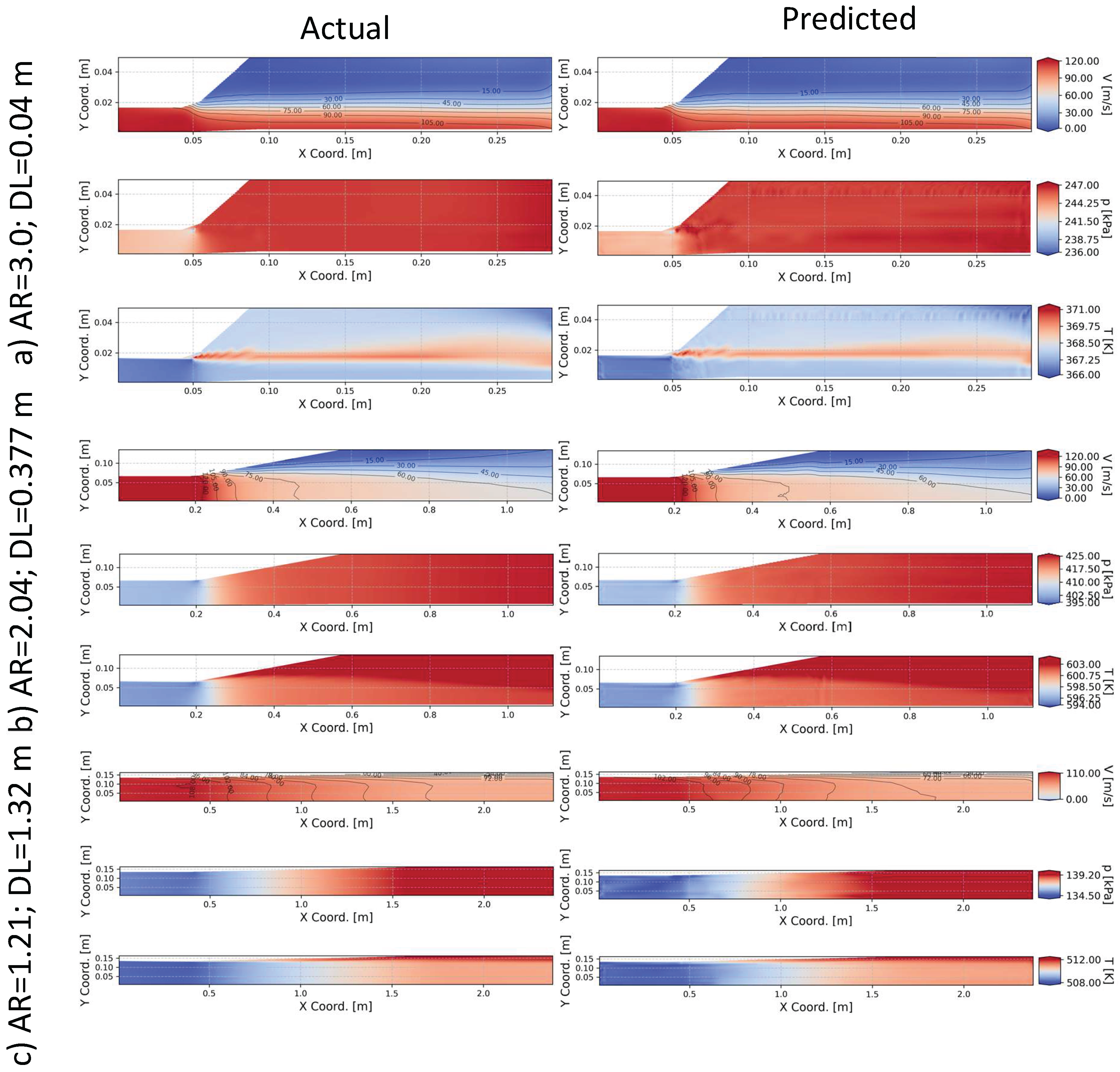
Figure 10.
Actual and predicted contours for testing dataset. a) Largest AR with shortest DL case, b) closest to the mean AR and DL of the dataset case and c) smallest AR and largest DL case.
Figure 10.
Actual and predicted contours for testing dataset. a) Largest AR with shortest DL case, b) closest to the mean AR and DL of the dataset case and c) smallest AR and largest DL case.
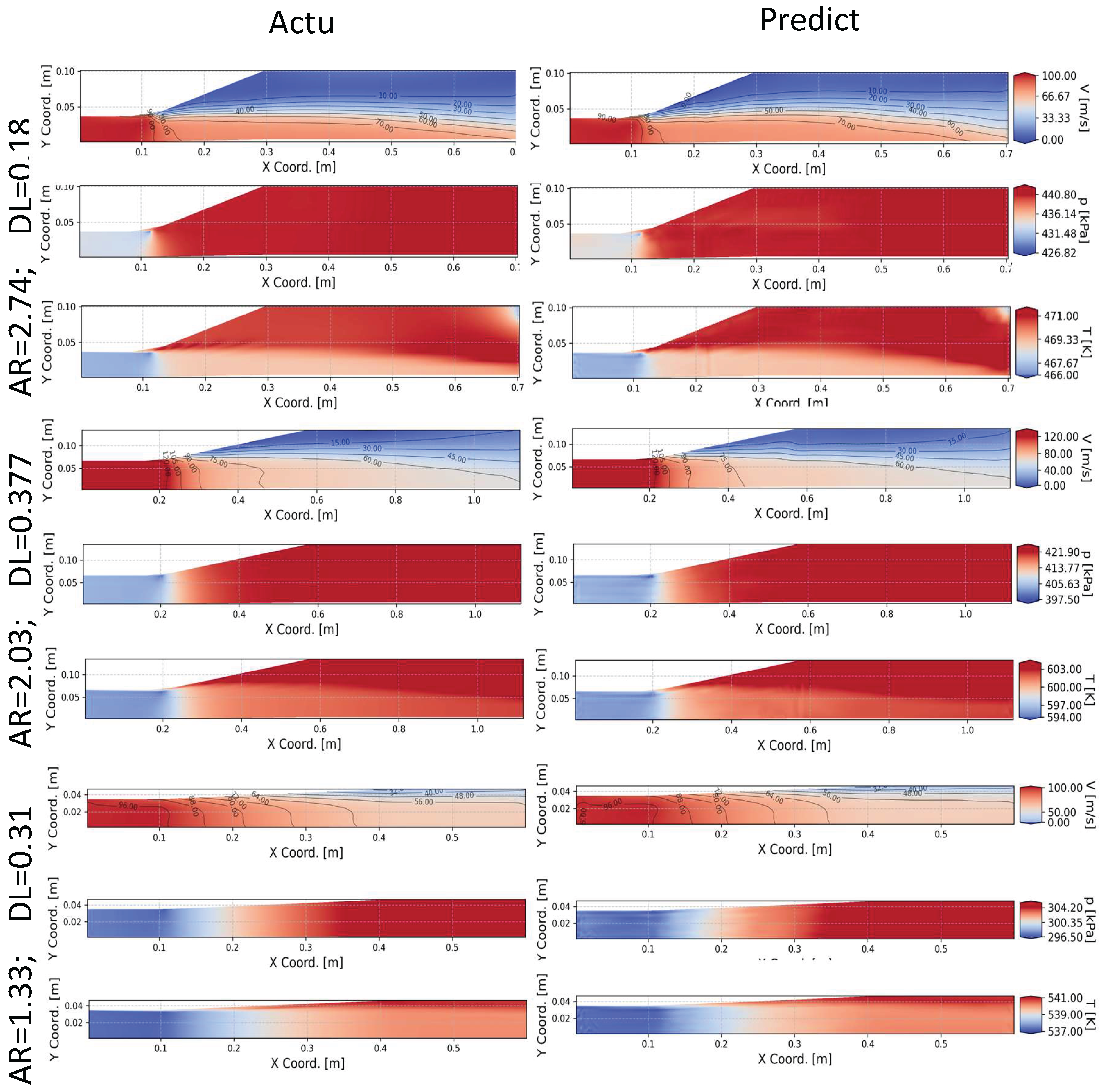

Table 1.
Design of experiment ranges for input parameters.
| Input parameter | Min | Max | Units |
|---|---|---|---|
| Inlet radius, | 0.01 | 0.15 | m |
| Aspect ratio, | 1.2 | 3 | - |
| Diffuser length, | 0.02 | 1.4 | m |
| Inlet velocity, | 30 | 150 | m/s |
| Outlet static pressure, | 100 | 500 | kPa |
| Inlet static temperature, | 298 | 600 | K |
Table 2.
Training and testing error metrics for evaluated architectures (cell contours formatted per column).
Table 2.
Training and testing error metrics for evaluated architectures (cell contours formatted per column).
| Training | Testing | ||||||||
|---|---|---|---|---|---|---|---|---|---|
| Index | Architecture short description | MSE | V-NMAPE | p-NMAPE | T-NMAPE | MSE | V-NMAPE | p-NMAPE | T-NMAPE |
| 1 | Pooling of GCN layer output and summing with FC layer output. Upscaling summed signal for next GCN layer. | 6,31E-04 | 4,960% | 0,172% | 0,049% | 1,50E-03 | 6,250% | 0,214% | 0,063% |
| 2 | Upscaling of FC output and summing with GCN layer output. Pooling summed signal for next FC layer. | 3,08E-04 | 3,400% | 0,110% | 0,037% | 1,90E-03 | 7,500% | 0,185% | 0,082% |
| 3 | Index 1 + concatenation of FC and GCN signals rather than summing. | 2,75E-04 | 3,370% | 0,099% | 0,037% | 1,04E-03 | 5,100% | 0,130% | 0,057% |
| 4 | Index 2 + concatenation of FC and GCN signals rather than summing. | 3,57E-04 | 4,840% | 0,138% | 0,050% | 2,01E-03 | 7,790% | 0,193% | 0,079% |
| 5 | Index 3 + residual connections. | 2,38E-04 | 3,020% | 0,100% | 0,037% | 9,65E-04 | 4,710% | 0,120% | 0,052% |
| 6 | Index 2 + residual connections. | 3,21E-04 | 3,59% | 0,12% | 0,04% | 1,44E-03 | 6,05% | 0,19% | 0,07% |
| 7 | Index 5 + layer normalization. | 3,09E-04 | 6,48% | 0,22% | 0,07% | 1,49E-03 | 7,21% | 0,23% | 0,08% |
| 8 | Index 6 + layer normalization. | 7,21E-04 | 11,32% | 0,28% | 0,10% | 1,49E-03 | 10,56% | 0,27% | 0,09% |
Table 3.
Training and testing MSEs for different numbers of network layers and hidden neurons using A5.
Table 3.
Training and testing MSEs for different numbers of network layers and hidden neurons using A5.
| Number of neurons per layer | 64 | 128 | 256 | 512 | 64 | 128 | 256 | 512 |
|---|---|---|---|---|---|---|---|---|
| Number of shared and GCN layers | Train MSE | Test MSE | ||||||
| x2 shared x3 GCN | 3,18E-04 | 2,11E-04 | 1,94E-04 | 2,03E-04 | 1,22E-03 | 9,60E-04 | 9,66E-04 | 1,03E-03 |
| x2 shared x5 GCN | 2,26E-04 | 1,72E-04 | 1,81E-04 | 1,36E-04 | 1,01E-03 | 1,17E-03 | 1,08E-03 | 1,08E-03 |
| x4 shared x3 GCN | 2,50E-04 | 1,91E-04 | 1,94E-04 | 1,49E-04 | 9,77E-04 | 9,80E-04 | 1,03E-03 | 9,40E-04 |
| x4 shared x5 GCN | 2,32E-04 | 1,67E-04 | 1,54E-04 | 1,33E-04 | 9,75E-04 | 1,01E-03 | 1,00E-03 | 9,10E-04 |
Table 4.
Training and testing MSEs and NMAPEs obtained for different number of nodal connections using A5.
Table 4.
Training and testing MSEs and NMAPEs obtained for different number of nodal connections using A5.
| Number of neighbours (graph density) | Training | Testing | ||
|---|---|---|---|---|
| MSE | V-NMAPE | MSE | V-NMAPE | |
| 4 | 1,67E-04 | 2,01% | 8,80E-04 | 3,90% |
| 8 | 1,05E-04 | 1,93% | 9,88E-04 | 4,07% |
| 16 | 1,84E-04 | 2,43% | 9,06E-04 | 4,39% |
Disclaimer/Publisher’s Note: The statements, opinions and data contained in all publications are solely those of the individual author(s) and contributor(s) and not of MDPI and/or the editor(s). MDPI and/or the editor(s) disclaim responsibility for any injury to people or property resulting from any ideas, methods, instructions or products referred to in the content. |
© 2025 by the authors. Licensee MDPI, Basel, Switzerland. This article is an open access article distributed under the terms and conditions of the Creative Commons Attribution (CC BY) license (http://creativecommons.org/licenses/by/4.0/).
Copyright: This open access article is published under a Creative Commons CC BY 4.0 license, which permit the free download, distribution, and reuse, provided that the author and preprint are cited in any reuse.


