
Submitted:
16 October 2025
Posted:
16 October 2025
You are already at the latest version
Abstract
The development of stable, accurate, and generalizable numerical simulation methods remains a critical challenge in computational fluid dynamics (CFD). Recently, physics-informed neural networks (PINNs) have emerged as a promising approach by embedding physical laws directly into the loss function of neural networks, enabling mesh-free solutions of governing equations. PINNs offer a new perspective on CFD and open a significant pathway for AI for science. However, existing PINN models often face trade-offs between generality, stability, and accuracy. To address these trade-offs, this paper proposes a novel hybrid architecture, PINN-MRT, which integrates the multi-relaxation-time lattice Boltzmann method (MRT-LBM) with PINNs. For the first time, the MRT-LBM evolution equation is embedded as the physics-informed residual within the loss function. Due to the mesoscopic kinetic nature of the MRT-LBM equations, the proposed PINN-MRT inherently possesses the potential for fluid solution generality. The PINN-MRT adopts a dual-network architecture, which separately predicts macroscopic conserved variables and
non-equilibrium distribution functions. A composite loss function is then constructed to incorporate physical residuals, boundary conditions, and data-driven terms, enabling the PINN-MRT architecture to simultaneously address both forward and inverse problems. Numerical validation on both forward and inverse problems confirms the superior stability and predictive accuracy of the proposed PINN-MRT model, demonstrating significant improvements over the standard PINN and existing PINN-LBM hybrid architectures. This study provides a novel stable, accurate, and generalizable PINN architecture for CFD research.
Keywords:
physics-informed neural networks
; multi-relaxation-time lattice Boltzmann method
; computational fluid dynamics
; deep learning
1. Introduction
Developing stable, accurate, and generalizable numerical simulation methods has long been one of the core challenges in computational fluid dynamics (CFD) [1,2,3]. Traditional numerical methods, such as the finite difference method (FDM), finite volume method (FVM), and spectral method (SM), have established the basic framework of modern CFD through discretization theory, mesh partitioning, and algebraic equation solving [1,4]. These methods have become benchmark tools for simulating physical phenomena such as fluid dynamics and heat transfer. However, when dealing with strong nonlinearity, discontinuous solutions, and complicated geometries, these traditional methods face significant limitations, including heavy reliance on refined meshes, numerical instability, and severe accuracy degradation or even failure [5,6,7].
In recent years, physics-informed neural networks (PINNs) have emerged as a novel computational method that combines the advantages of physical laws and data-driven learning [8]. Leveraging the mesh-free computation, PINNs demonstrate great potential in addressing diverse fluid problems, gradually becoming a key new paradigm to break through the bottlenecks of traditional numerical methods [9]. Specifically, PINNs embed physical laws directly into the loss function of neural networks and utilize parameter optimization to implicitly solve the governing equations, thus largely eliminating mesh dependence and enhancing adaptability to complex physical problems [10,11,12]. For instance, this approach has demonstrated excellent performance in shock capturing, turbulence modeling, and unsteady flow simulations [13]. Nonetheless, PINNs also suffer from challenges including the emergence of spurious solutions, convergence difficulties, and limited capability for dynamic system modeling [10,14,15]. As a result, introducing hybrid model architectures to improve robustness has become a promising research direction. Among these approaches, the integration of PINNs with the lattice Boltzmann method (LBM) represents a recently developed research direction.
The LBM, owing to its clear evolution mechanism, highly parallel computational structure, and flexibility in handling intricate boundaries and multi-physics coupling problems, has been widely adopted for numerical simulation in CFD [16]. Its fundamental governing equation, the lattice Boltzmann equation (LBE), originates from the underlying kinetic equation, i.e., the continuous Boltzmann equation. This intrinsic physical nature rooted in kinetic theory enables the LBE to systematically preserve the essential coupling between microscopic particle dynamics and macroscopic conservation law evolution in physical modeling, thus endowing it with inherent physical consistency, theoretical closure, and high generality for fluid flow solutions [17,18]. The LBE models the mesoscopic evolution of particle distributions through collision and streaming processes, and offers a solid theoretical basis for complex flow simulations.
Based on this, some researchers have proposed combining LBM with PINNs, replacing conventional partial differential equations, such as Navier-Stokes (N-S) equations, with the LBE as the underlying governing equations, thereby constructing hybrid models that integrate mesoscopic physical constraints [19]. For example, Lou et al. proposed a PINN architecture incorporating the Boltzmann-Bhatnagar-Gross-Krook (BGK) equation, substantially enhancing the model physical accuracy, and alleviating issues such as slow convergence and difficulties in modeling highly nonlinear scenarios [20]. However, due to coupling the relaxation of all hydrodynamic and non-hydrodynamic moments to a single parameter, the BGK model exhibits severe parameter coupling and numerical instability in flow simulations, thus limiting its applicability in complex scenarios [16,17].
To address these challenges, this paper proposes a PINN architecture incorporating the multi-relaxation-time lattice Boltzmann method (MRT-LBM). The MRT collision mechanism effectively decouples the relaxation processes of different order momentum components by assigning independent relaxation time to each physical mode [21,22]. This approach retains the advantages of mesoscale modeling while markedly improving the accuracy, numerical stability, and generalizability for diverse fluid structures. The remainder of this paper is organized as follows: Section 2 presents the theoretical foundation, along with the design of the proposed PINN-MRT architecture that integrates dual-network and physics-informed loss functions. Section 3 introduces the benchmark problem setup and model configurations. Section 4 demonstrates the applications of PINN-MRT to forward and inverse problems, including predictive accuracy and parameter identification at different Reynolds numbers (Re). Finally, Section 5 summarizes the main findings and outlines future research directions.
2. Method
2.1. MRT-LBM
The LBM is an efficient numerical simulation approach at the mesoscopic scale, describing the statistical evolution of particle distribution functions through discretization in both space and time, as well as along specific discrete velocity directions. The fundamental dynamical model of LBM originates from the continuous Boltzmann equation [23]
where f denotes the particle distribution function in continuous velocity space, represents the microscopic particle velocity, and is the collision operator, characterizing the relaxation process toward local equilibrium. A classical simplification is the single-relaxation-time (SRT) or BGK approximation, which linearizes the collision operator to model the relaxation process toward a local equilibrium distribution function [24]
In Eq.2, denotes the single relaxation factor, which directly determines the fluid kinematic viscosity, and represents the equilibrium distribution function. However, the SRT model employs a unified relaxation parameter across all dynamical moments, which inherently leads to strong coupling among different physical processes and restricts the flexibility in independently controlling individual transport phenomena [24]. Fortunately, the MRT model introduces a transformation into moment space assigning independent relaxation parameters to distinct physical modes (mass, momentum, stress, etc.). The corresponding equation is shown as [25,26]
where denotes an orthogonal transformation matrix that maps f from velocity space to moment space, and is a diagonal matrix whose elements correspond to the relaxation times associated with individual moments. The D2Q9 discrete velocity model is adopted, and the resulting discretized evolution equation is given by
where is the particle distribution function. is the equilibrium discrete distribution function, and for the D2Q9 discrete velocity model can be expressed as
where is weight coefficients in the ith direction, which is given by
The macroscopic fluid density and macroscopic fluid velocity are shown as [27]
where discrete velocity along the ith direction. In this study, is given by
The orthogonal transformation matrix is expressed as [27]
The diagonal relaxation matrix is shown as
where , , , , , and represent the relaxation factors associated with density, energy, square root of energy, momentum flux component, energy flux component, and pressure tensor, respectively. In this study, the relaxation factors are set as follows, , , and . In the MRT model, the kinematic viscosity is related to the relaxation factor by
where denotes the lattice sound speed, with in the D2Q9 model. is the time step.
2.2. PINN-MRT
A novel architecture (PINN-MRT) is developed in this study by integrating MRT-LBM into the PINNs architecture. As shown in Figure 1, the PINN-MRT architecture comprises two main components, i.e. the neural network architecture and the loss function design.
2.2.1. Neural Network Architecture
The neural network architecture has two sub-networks. The first sub-network, denoted as , takes the spatial coordinates as input and outputs the macroscopic density and velocity components , then calculates the equilibrium distribution function using Eq.6. The second sub-network, , shares the same input as but predicts the nine components of the non-equilibrium distribution function . This physically motivated separation leverages the smoothness of and the complexity of , allowing each network to focus on distinct features and thereby improving stability and accuracy [28].
Based on the predicted outputs, the total distribution function at each spatial location is composed as
2.2.2. Loss Function Design
For effective training of the PINN-MRT model, a loss function is formulated incorporating the physical residuals, boundary conditions, initial conditions, and data-driven terms, as shown in Eq.14 [29].
where denote the weight coefficients corresponding to the respective loss components. To ensure consistency in comparisons with other models, this study does not implement weight optimization and instead adopts unit weight coefficients (i.e., ) for active loss terms, while setting for unused components.
The physics residual loss ensures that the neural network predictions satisfy the governing dynamics derived from the MRT-LBM equations. The specific equation can be expressed as [30]
where denotes the residual of the MRT-LBM evolution in the i-th discrete velocity direction, Q refers to the total number of discrete velocity directions, and and specify the numbers of temporal and internal sampling points, respectively. The spatial coordinate for the j-th sampling point is given by , with representing its corresponding temporal coordinate.
The boundary condition loss is introduced to enforce that the predicted solutions strictly satisfy the prescribed boundary conditions, thereby ensuring physical consistency at the domain boundaries. In the LBM kinetic framework, it is further divided into three components
- Macroscopic boundary loss : Constrains the predicted macroscopic variables on the boundaries to match the prescribed physical values.
- Distribution function consistency loss : Constrains the predicted equilibrium and non-equilibrium distribution functions to match the theoretically defined boundary distributions.
- Boundary PDE residual loss : Imposes constraints on the neural network outputs by penalizing the residuals of the governing equations at the boundaries.
The equations for the three components are given by
Thus, the formula for is
In Eq.17, where denotes the predicted macroscopic physical quantities (e.g., velocity or density), represents the ground truth boundary condition, is the number of boundary sampling points, and and denote the spatial and temporal coordinates, respectively, of the j-th boundary point. In Eq.18, represents the non-equilibrium distribution function in the i-th discrete velocity direction predicted by the neural network, is the theoretical reference value at the boundary, and indicates that only outgoing velocity directions are considered (from the interior to the boundary). Eq.19 indicates that the evolution equation in the incident direction remains enforced at the boundary.
The initial condition loss ensures that the predicted initial state strictly conforms to the known reference solution. The equation is given by
with representing the number of sampling points.
The data-driven loss minimizes the discrepancy between the predicted values and the experimentally measured or observed data. It is defined as
where denotes the total number of data points, represents the observed velocity data, thereby guiding the neural network to better approximate the actual physical data.
3. Benchmark Modeling
The classical lid-driven cavity flow is selected as the benchmark case to evaluate the model performance. As shown in Figure 2, the computational domain is a unit square with spatial coordinates . A constant velocity of , is prescribed on the top boundary, and the remaining walls are subjected to no-slip conditions (i.e., stationary). This setup induces a characteristic steady-state vortex structure that varies with Re, making it a widely adopted benchmark for assessing the predictive capability of both forward and inverse modeling approaches. The specific governing equations are written as [31]
where denote the velocity components in the x and y directions, respectively, p is the pressure, and represents the kinematic viscosity, which can be expressed in terms of the Re as
here, U represents the lid velocity, and L denotes the characteristic length (i.e., the cavity length).
These governing equations are formulated from the general N-S equations under steady-state, incompressible, and two-dimensional assumptions.
To rigorously evaluate the performance of the proposed PINN-MRT architecture, two benchmark models are established for comparative analysis. All models share the same network architecture and training configuration, differing solely in the formulation of the residual term ,which encodes the respective physical constraints [32]. The standard PINN adopts Eq.23 as its macroscopic residual constraints. Meanwhile, PINN-SRT introduces mesoscopic physical constraints based on SRT equation, which can be regarded as a special case of the MRT model when all the diagonal elements of the relaxation matrix are set to unity [32].
The detailed configurations for each model in inverse problem are listed in Table 1. The training data are obtained by solving Eq.23 using the traditional FDM, which also provides the reference numerical solutions for comparison in Section.Section 4.
Table 2 summarizes the corresponding configurations for forward problem. In this context, all physical parameters are known, and no additional data are introduced. A deeper network architecture (7-layers) is adopted to handle this more challenging data-free prediction task. Meanwhile, the sub-network for the non-equilibrium part uses more neurons (100 vs. 60) to better capture complex local features [10,14,33,34].
4. Results
4.1. Inverse Problem
The subsequent analysis of the inverse problem is divided into two parts: Flow Field Analysis, focusing on the reconstruction of physical fields, and Parameter Inversion, addressing the identification of underlying model parameters.
4.1.1. Flow Field Analysis
The comprehensive performance comparison among the standard PINN, PINN-SRT and PINN-MRT models is conducted up to Re = 1000, since the standard PINN and PINN-SRT models become numerically unstable and fail to produce reliable results when the Re exceeds 1000. In this range, all models are systematically analyzed in terms of vortex structure reconstruction, error distribution, and velocity profile consistency. To further verify the robustness of the PINN-MRT model under more challenging flow conditions, additional evaluations at Re = 2000 and 5000 are conducted exclusively for the PINN-MRT model.
(A) Vortex Structure Reconstruction and Error Distribution
Figure 3 illustrates the predicted u and v velocity fields at Re = 100, showing small differences among three models. The absolute error (Abs) distributions in Figure 4 further confirm this observation. While the errors of all three models remain comparably low, PINN-MRT achieves the smallest and most localized errors. These results motivate further exploration at higher Re.
Figure 5 presents the flow field results at Re = 1000, where more complex structures appear compared to low Re. The primary vortex is mainly identified in the u velocity field as a large central rotational structure, whereas the secondary vortices are clearly observed in the v velocity field near the bottom corners. Among the models, the PINN-MRT accurately reconstructs both primary and secondary flow structures features, capturing their rotational directions and spatial distributions. By comparison, the PINN-SRT partially recovers the primary vortex but fails to resolve the secondary features. The standard PINN exhibits a complete breakdown in prediction. As shown in Figure 6, the PINN-MRT maintains low error levels, with peaks errors below 0.10 for u and 0.15 for v. Meanwhile, the PINN-SRT reaches peak errors of 0.30 with wider distributions, and the standard PINN yields errors exceeding 0.40, indicating clear failure.
(B) Velocity Profile
Centerline velocity profiles are analyzed to evaluate the accuracy of flow reconstruction along key directions. Table 3 summarizes the absolute error ranges of the horizontal and vertical velocity components for Re = 100 and 1000. The PINN-MRT model achieves the narrowest error bounds in both directions, confirming its superior predictive accuracy.
(C) High-Re Error Evaluation of PINN-MRT
The summarized relative errors of the PINN-MRT model across all tested Re are presented in Table 4. Here, and represent the horizontal and vertical velocity component errors, respectively, and denotes the total velocity magnitude error. As the Re increases from 100 to 5000, the errors naturally rise, with increasing from 9.067% to 15.281%, from 11.942% to 21.262%, and from 4.549% to 14.121%. Nevertheless, the error levels remain well controlled, demonstrating the robustness and practical applicability of the PINN-MRT model.
4.1.2. Parameter Inversion
Building on the successful flow field reconstruction, the proposed PINN-MRT model is further assessed for its capability in parameter inversion, focusing on both the kinematic viscosity coefficient and the lid velocity . The inversion accuracy is systematically compared among the standard PINN, PINN-SRT, and PINN-MRT models across Reynolds numbers ranging from to 5000, as well as under noise-contaminated conditions.
As shown in Figure 7, the left panels present the relative errors of the inferred and for different models, while the right panels illustrate the corresponding robustness tests with noisy data, where the shaded regions denote a uncertainty band.
For the noiseless cases (left column), both PINN and PINN-SRT exhibit a rapid degradation of accuracy as Re increases, with relative errors exceeding and , respectively, at . In contrast, the PINN-MRT maintains errors below for both parameters across the entire Reynolds number range, demonstrating remarkable stability and resistance to ill-conditioning at high Reynolds numbers.
Under noisy inputs (right column), the PINN-MRT results remain within the confidence interval, showing only marginal increases in error. This confirms that the MRT-based regularization effectively suppresses the amplification of noise during inverse inference, thereby ensuring both robustness and consistency of the reconstructed physical parameters.
4.2. Forward Problem
4.2.1. Flow Field Analysis
The forward problem focuses on evaluating the capability of each model to predict steady-state flow fields given known physical parameters. In this scenario, no additional data-driven constraints are introduced. Comparative evaluations are conducted at Re = 100 and 400 for all models (PINN, PINN-SRT, and PINN-MRT). For higher Re (Re > 400), only the PINN-MRT model is considered, as the other two models fail to produce reliable predictions under these more challenging conditions.
(A) Vortex Structure Reconstruction and Error Distribution
As shown in Figure 9, at Re = 100, the absolute error distributions demonstrate that the PINN-MRT model achieves the lowest error levels, highlighting its superior accuracy under low Re conditions.
At Re = 400 (Figure 11), the absolute error distributions clearly illustrate significant performance differences among the models. Compared to Re = 100, the errors of the PINN-MRT model show a slight increase. In contrast, both the standard PINN and PINN-SRT models have completely failed.
(B) Velocity Profile
As summarized in Table 5, at Re = 100, both the standard PINN and PINN-SRT models exhibit error ranges in and approximately twice as large as those of PINN-MRT. When Re increases to 400, the of PINN reaches nearly three times, and that of PINN-SRT about five times, compared to PINN-MRT. For , the errors are even more pronounced, with PINN and PINN-SRT reaching approximately seven and six times larger than PINN-MRT, respectively.
(C) High Re Error Evaluation of PINN-MRT
As presented in Table 6, the PINN-MRT model performs robustly across all tested conditions. Notably, the increase in the vertical velocity component error is minimal, only 1.801% across the entire Re range. The horizontal velocity and total velocity component errors exhibit increases of approximately 5.000%. These restrained error increments underscore the model’s robust stability and accuracy, even under high Re conditions.
4.2.2. Viscosity Sensitivity
To further evaluate the stability of the model with respect to parameter perturbations, a sensitivity study was conducted by introducing controlled variations in the kinematic viscosity coefficient . Figure 12 presents the relative errors of the reconstructed velocity fields (u, v, and total) under viscosity perturbations ranging from to for different Reynolds numbers. The shaded regions represent uncertainty bands.
Across all cases, the PINN-MRT model maintains stable error levels, with total relative errors remaining within the range, indicating low sensitivity to variations in . The v-component shows relatively higher errors than u, particularly at higher Reynolds numbers. This behavior is attributed to the weak vertical velocity magnitude and the strong secondary vortex effects in the lid-driven cavity flow, which amplify relative deviations when minor physical perturbations occur. Overall, the results confirm that the proposed PINN-MRT framework achieves consistent flow reconstruction accuracy and robustness against viscosity perturbations in the forward modeling task.
5. Conclusions
In this study, the proposed PINN-MRT model is systematically applied to both forward and inverse problems, covering Re ranging from 100 to 5000. For inverse problems, it achieves high-fidelity parameter identification and flow field reconstruction, with remarkable robustness. For forward problems, the architecture exhibits outstanding predictive accuracy, precisely capturing intricate flow structures and velocity profiles. In addition, a sensitivity analysis on the kinematic viscosity demonstrates that the model maintains stable convergence under perturbations, confirming its insensitivity to small variations in physical parameters. These results highlight the robustness and predictive accuracy of the PINN-MRT framework across a broad range of flow conditions, including challenging high Re scenarios.
The primary contribution of this study is the introduction of the MRT collision mechanism into the PINN architecture. By assigning independent relaxation factors to different moment components, this approach effectively mitigates the critical trade-offs between stability, accuracy, and generalization that often constrains conventional PINN methods. This leads to a significant enhancement in the overall robustness and convergence of the training process.
It is worth noting that the current implementation employs basic fully connected networks, simple optimization strategies, and the fundamental MRT formulation.
In future work, this framework can be further improved by leveraging advanced neural architectures and more efficient training strategies to enhance convergence and scalability. For example, adaptive weighting mechanisms and dynamic optimization schemes will be introduced to better balance multiple loss components and improve numerical stability. Exploring advanced PINN variants, such as XPINNs [35], PDPINNs [36], and GPINNs [37], will also extend the applicability of the framework to high-dimensional and noisy flow systems. Furthermore, the PINN-MRT architecture can be extended through integrating specialized physics modules, such as pseudopotential models for multiphase and multicomponent flows, thermal formulations for heat transfer problems, and advanced boundary schemes for complex geometries. These extensions are expected to improve the capability of the framework to resolve complex interactions such as multiphase interfaces, thermal effects, and multiscale dynamics, while the pursuit of higher generalizability remains a key objective. In summary, the PINN-MRT model can be viewed as a bridge between LBM and deep learning, offering a promising foundation upon which more sophisticated and robust hybrid models can be built in future research.
Data Availability Statement
The data that support the findings of this study are available from the corresponding author upon reasonable request.
Acknowledgments
The authors are grateful for the valuable comments and suggestions from the respected reviewers, which have greatly enhanced the quality and significance of this work. Financial support from the National Natural Science Foundation of China (Grant Nos. 12474453, 12174085, and 12404530) is also gratefully acknowledged.
Conflicts of Interest
The authors have no conflicts to disclose.
References
- Runchal, A.K. Evolution of CFD as an engineering science. A personal perspective with emphasis on the finite volume method. Comptes Rendus. Mécanique 2022, 350, 233–258. [Google Scholar] [CrossRef]
- Ranganathan, P.; Pandey, A.K.; Sirohi, R.; Hoang, A.T.; Kim, S.H. Recent advances in computational fluid dynamics (CFD) modelling of photobioreactors: Design and applications. Bioresource technology 2022, 350, 126920. [Google Scholar] [CrossRef]
- Lee, S.; Zhao, Y.; Luo, J.; Zou, J.; Zhang, J.; Zheng, Y.; Zhang, Y. A review of flow control strategies for supersonic/hypersonic fluid dynamics. Aerospace Research Communications 2024, 2, 13149. [Google Scholar] [CrossRef]
- Tu, J.; Yeoh, G.H.; Liu, C.; Tao, Y. Computational fluid dynamics: a practical approach; Elsevier, 2023.
- Hafeez, M.B.; Krawczuk, M. A Review: Applications of the Spectral Finite Element Method: MB Hafeez and M. Krawczuk. Archives of Computational Methods in Engineering 2023, 30, 3453–3465. [Google Scholar] [CrossRef]
- Xu, H.; Cantwell, C.D.; Monteserin, C.; Eskilsson, C.; Engsig-Karup, A.P.; Sherwin, S.J. Spectral/hp element methods: Recent developments, applications, and perspectives. Journal of Hydrodynamics 2018, 30, 1–22. [Google Scholar] [CrossRef]
- Droniou, J. Finite volume schemes for diffusion equations: introduction to and review of modern methods. Mathematical Models and Methods in Applied Sciences 2014, 24, 1575–1619. [Google Scholar] [CrossRef]
- Raissi, M.; Perdikaris, P.; Karniadakis, G.E. Physics-informed neural networks: A deep learning framework for solving forward and inverse problems involving nonlinear partial differential equations. Journal of Computational physics 2019, 378, 686–707. [Google Scholar] [CrossRef]
- Rui, E.Z.; Zeng, G.Z.; Ni, Y.Q.; Chen, Z.W.; Hao, S. Time-averaged flow field reconstruction based on a multifidelity model using physics-informed neural network (PINN) and nonlinear information fusion. International Journal of Numerical Methods for Heat & Fluid Flow 2024, 34, 131–149. [Google Scholar]
- Karniadakis, G.E.; Kevrekidis, I.G.; Lu, L.; Perdikaris, P.; Wang, S.; Yang, L. Physics-informed machine learning. Nature Reviews Physics 2021, 3, 422–440. [Google Scholar] [CrossRef]
- Liu, B.; Wei, J.; Kang, L.; Liu, Y.; Rao, X. Physics-informed neural network (PINNs) for convection equations in polymer flooding reservoirs. Physics of Fluids 2025, 37. [Google Scholar] [CrossRef]
- Wong, J.C.; Gupta, A.; Ong, Y.S. Can transfer neuroevolution tractably solve your differential equations? IEEE Computational Intelligence Magazine 2021, 16, 14–30. [Google Scholar] [CrossRef]
- Willard, J.; Jia, X.; Xu, S.; Steinbach, M.; Kumar, V. Integrating scientific knowledge with machine learning for engineering and environmental systems. ACM Computing Surveys 2022, 55, 1–37. [Google Scholar] [CrossRef]
- Lu, L.; Meng, X.; Mao, Z.; Karniadakis, G.E. DeepXDE: A deep learning library for solving differential equations. SIAM review 2021, 63, 208–228. [Google Scholar] [CrossRef]
- Lee, J.; Shin, S.; Kim, T.; Park, B.; Choi, H.; Lee, A.; Choi, M.; Lee, S. Physics informed neural networks for fluid flow analysis with repetitive parameter initialization. Scientific Reports 2025, 15, 16740. [Google Scholar] [CrossRef]
- d’Humieres, D. Generalized lattice-Boltzmann equations. Rarefied gas dynamics 1992. [Google Scholar]
- Guo, Z.; Shi, B.; Wang, N. Lattice BGK model for incompressible Navier–Stokes equation. Journal of Computational Physics 2000, 165, 288–306. [Google Scholar] [CrossRef]
- Chen, S.; Doolen, G.D. Lattice Boltzmann method for fluid flows. Annual review of fluid mechanics 1998, 30, 329–364. [Google Scholar] [CrossRef]
- Chen, Z.; Liu, Y.; Sun, H. Physics-informed learning of governing equations from scarce data. Nature communications 2021, 12, 6136. [Google Scholar] [CrossRef]
- Lou, Q.; Meng, X.; Karniadakis, G.E. Physics-informed neural networks for solving forward and inverse flow problems via the Boltzmann-BGK formulation. Journal of Computational Physics 2021, 447, 110676. [Google Scholar] [CrossRef]
- Shi, X.; Huang, X.; Zheng, Y.; Ji, T. A hybrid algorithm of lattice Boltzmann method and finite difference–based lattice Boltzmann method for viscous flows. International Journal for Numerical Methods in Fluids 2017, 85, 641–661. [Google Scholar] [CrossRef]
- Cheng, X.; Su, R.; Shen, X.; Deng, T.; Zhang, D.; Chang, D.; Zhang, B.; Qiu, S. Modeling of indoor airflow around thermal manikins by multiple-relaxation-time lattice Boltzmann method with LES approaches. Numerical Heat Transfer, Part A: Applications 2020, 77, 215–231. [Google Scholar] [CrossRef]
- Zheng, J.; Zha, Y.; Feng, M.; Shan, M.; Yang, Y.; Yin, C.; Han, Q. Numerical investigation on jet-enhancement effect and interaction of out-of-phase cavitation bubbles excited by thermal nucleation. Ultrasonics Sonochemistry, 1073. [Google Scholar]
- Chai, Z.; Shi, B.; Guo, Z. A multiple-relaxation-time lattice Boltzmann model for general nonlinear anisotropic convection–diffusion equations. Journal of Scientific Computing 2016, 69, 355–390. [Google Scholar] [CrossRef]
- Krüger, T.; Kusumaatmaja, H.; Kuzmin, A.; Shardt, O.; Silva, G.; Viggen, E.M. The lattice Boltzmann method; Vol. 10, Springer, 2017.
- Yang, Y.; Tu, J.; Shan, M.; Zhang, Z.; Chen, C.; Li, H. Acoustic cavitation dynamics of bubble clusters near solid wall: A multiphase lattice Boltzmann approach. Ultrasonics Sonochemistry 2025, 114, 107261. [Google Scholar] [CrossRef] [PubMed]
- Shan, M.; Zha, Y.; Yang, Y.; Yang, C.; Yin, C.; Han, Q. Morphological characteristics and cleaning effects of collapsing cavitation bubble in fractal cracks. Physics of Fluids 2024, 36. [Google Scholar] [CrossRef]
- Zhao, B.; Sun, D.; Wu, H.; Qin, C.; Fei, Q. Physics-informed neural networks for solcing inverse problems in phase field models. Neural Networks, 1076. [Google Scholar]
- Jagtap, A.D.; Mao, Z.; Adams, N.; Karniadakis, G.E. Physics-informed neural networks for inverse problems in supersonic flows. Journal of Computational Physics 2022, 466, 111402. [Google Scholar] [CrossRef]
- Lu, L.; Pestourie, R.; Yao, W.; Wang, Z.; Verdugo, F.; Johnson, S.G. Physics-informed neural networks with hard constraints for inverse design. SIAM Journal on Scientific Computing 2021, 43, B1105–B1132. [Google Scholar] [CrossRef]
- Jin, X.; Cai, S.; Li, H.; Karniadakis, G.E. NSFnets (Navier-Stokes flow nets): Physics-informed neural networks for the incompressible Navier-Stokes equations. Journal of Computational Physics 2021, 426, 109951. [Google Scholar] [CrossRef]
- Lallemand, P.; Luo, L.S. Theory of the lattice Boltzmann method: Dispersion, dissipation, isotropy, Galilean invariance, and stability. Phys. Rev. E 2000, 61, 6546–6562. [Google Scholar] [CrossRef]
- Markidis, S. The Old and the New: Can Physics-Informed Deep-Learning Replace Traditional Linear Solvers? 2021; arXiv:math.NA/2103.09655]. [Google Scholar]
- Hao, Z.; Yao, J.; Su, C.; Su, H.; Wang, Z.; Lu, F.; Xia, Z.; Zhang, Y.; Liu, S.; Lu, L.; et al. 2023; arXiv:cs.LG/2306.08827].
- Jagtap, A.D.; Karniadakis, G.E. Extended physics-informed neural networks (XPINNs): A generalized space-time domain decomposition based deep learning framework for nonlinear partial differential equations. Communications in Computational Physics 2020, 28. [Google Scholar] [CrossRef]
- Peng, W.; Zhou, W.; Zhang, J.; Yao, W. Accelerating physics-informed neural network training with prior dictionaries. arXiv preprint arXiv:2004.08151, arXiv:2004.08151 2020.
- Yu, J.; Lu, L.; Meng, X.; Karniadakis, G.E. Gradient-enhanced physics-informed neural networks for forward and inverse PDE problems. Computer Methods in Applied Mechanics and Engineering 2022, 393, 114823. [Google Scholar] [CrossRef]
Figure 1.
The presented PINN-MRT architecture with MRT-LBM physics constraints.
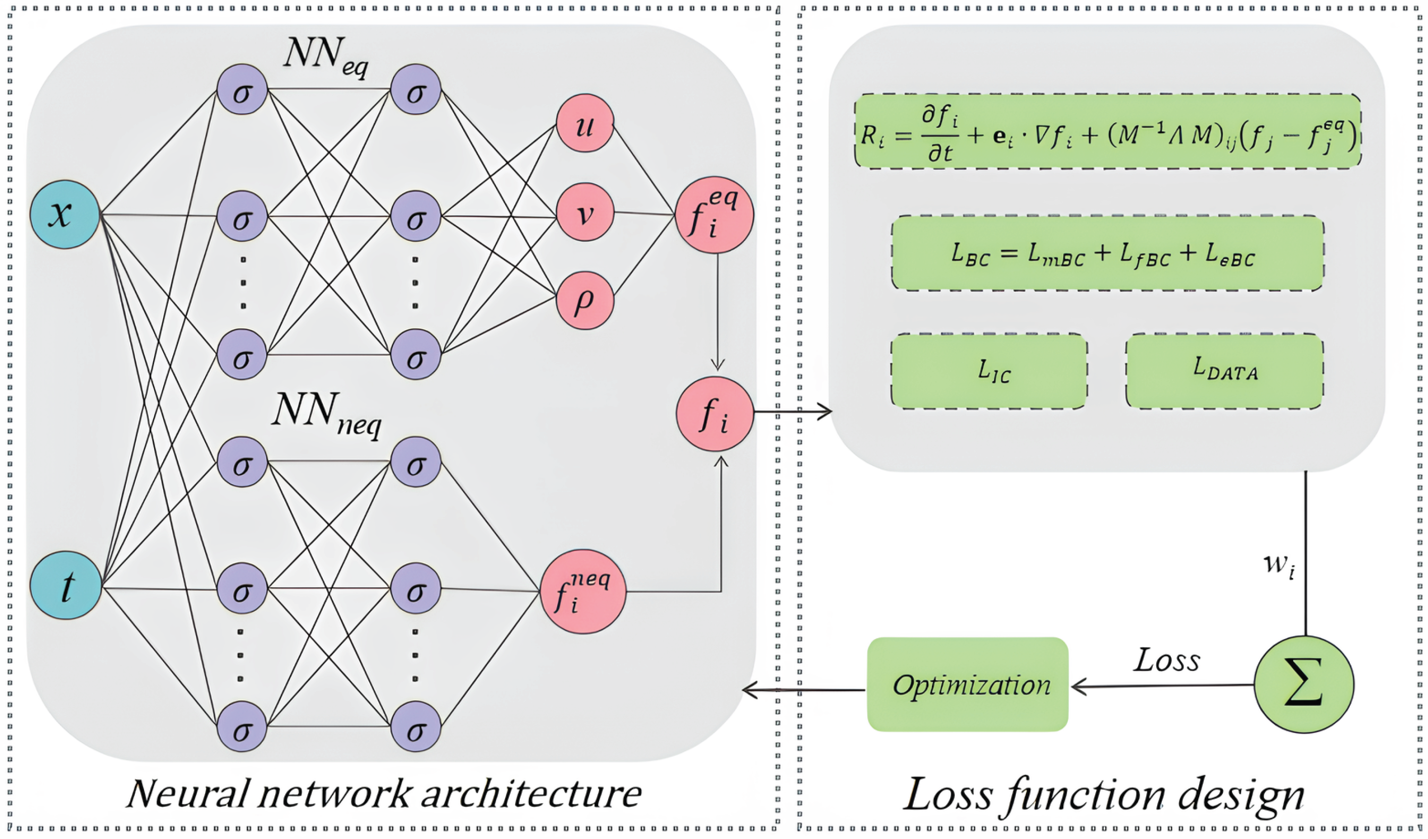
Figure 2.
2D computational domain and boundary conditions for the lid-driven cavity flow.
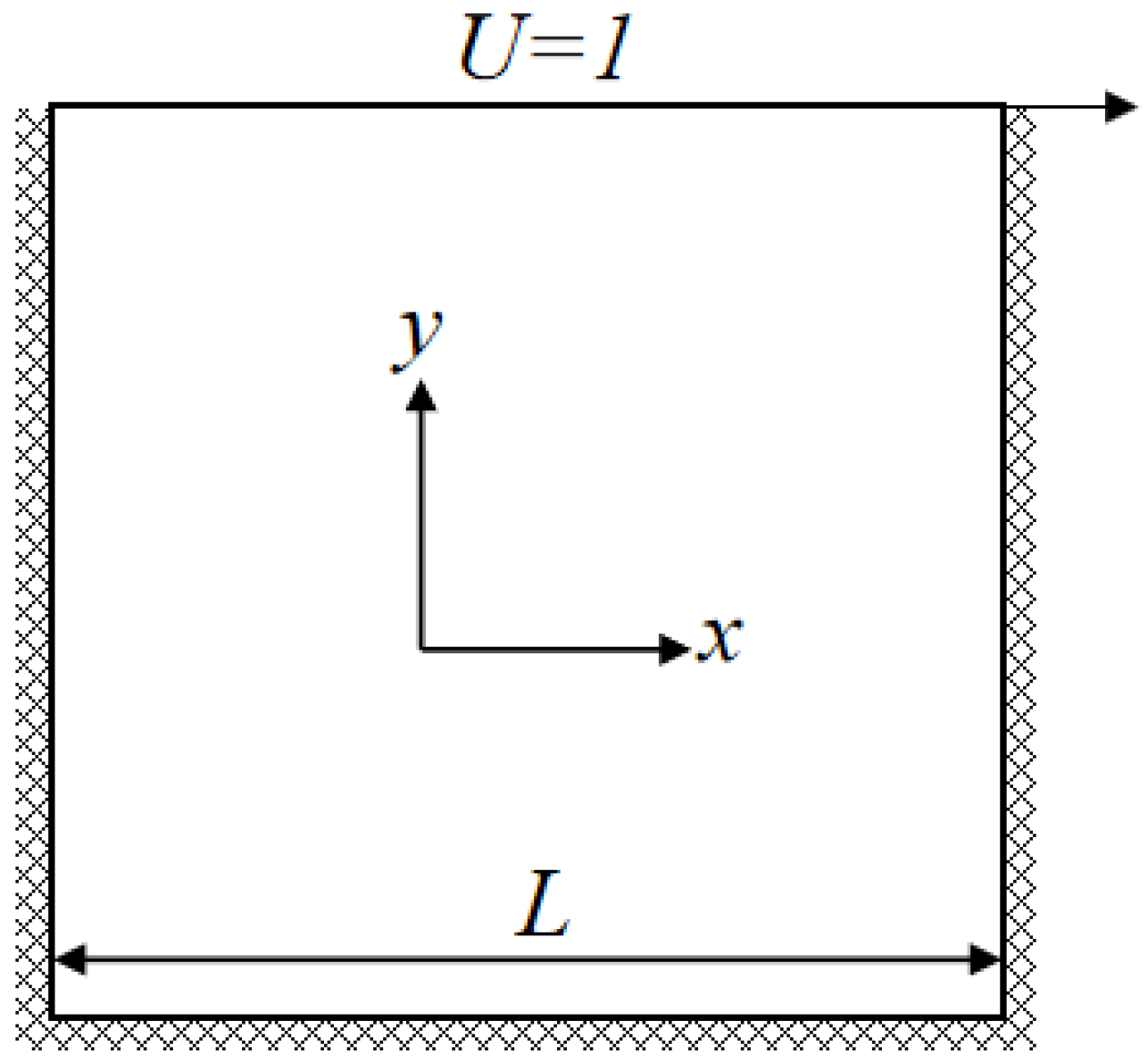
Figure 3.
Inverse problem solution comparison of velocity field at Re = 100.
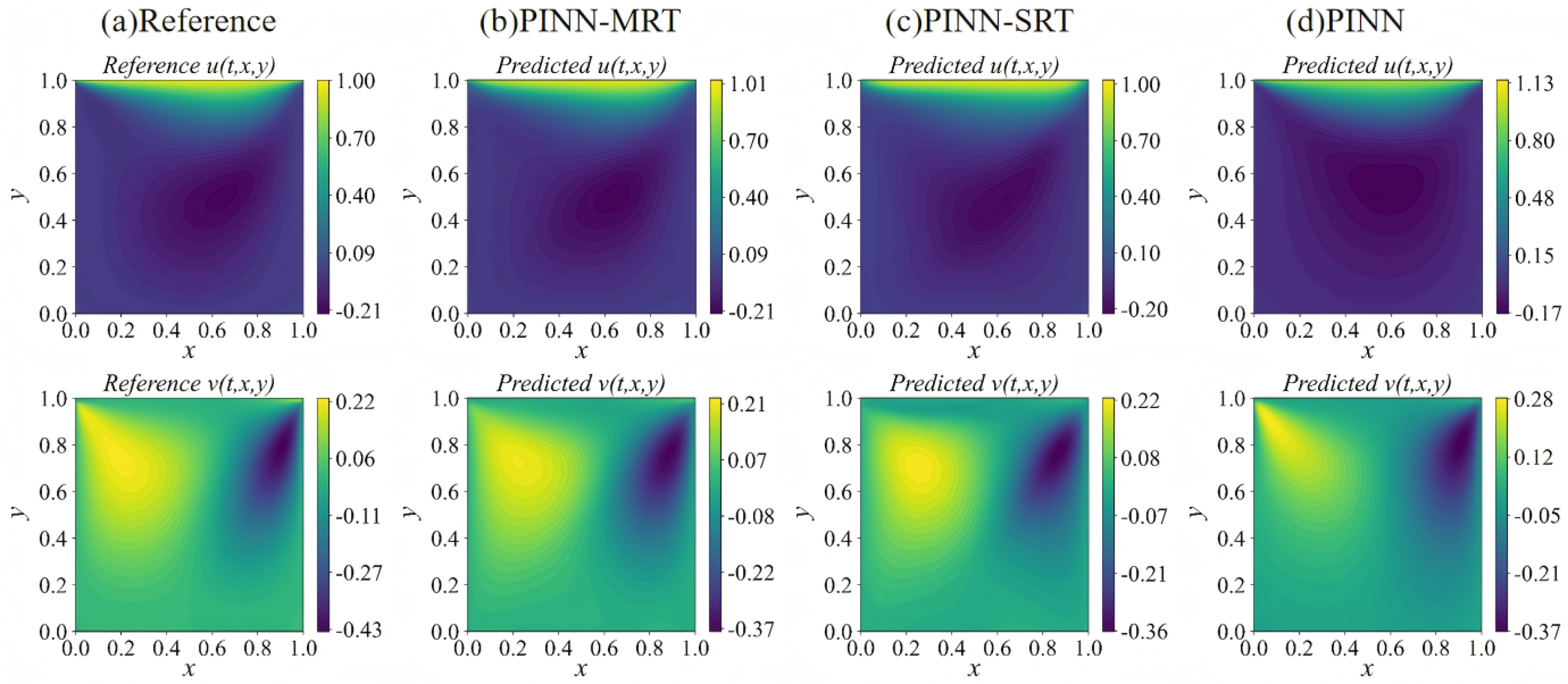
Figure 4.
Absolute error distributions of the velocity components u and v at Re = 100.
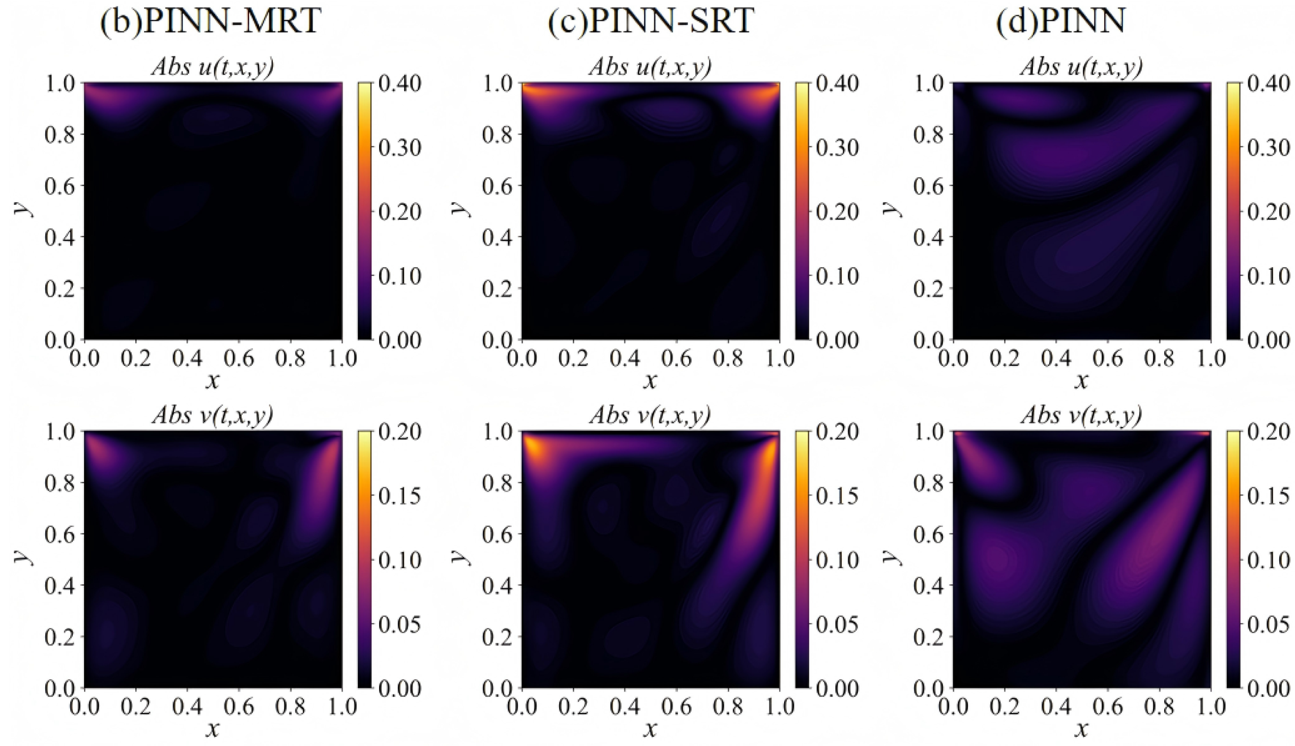
Figure 5.
Inverse problem solution comparison of velocity field at Re = 1000.
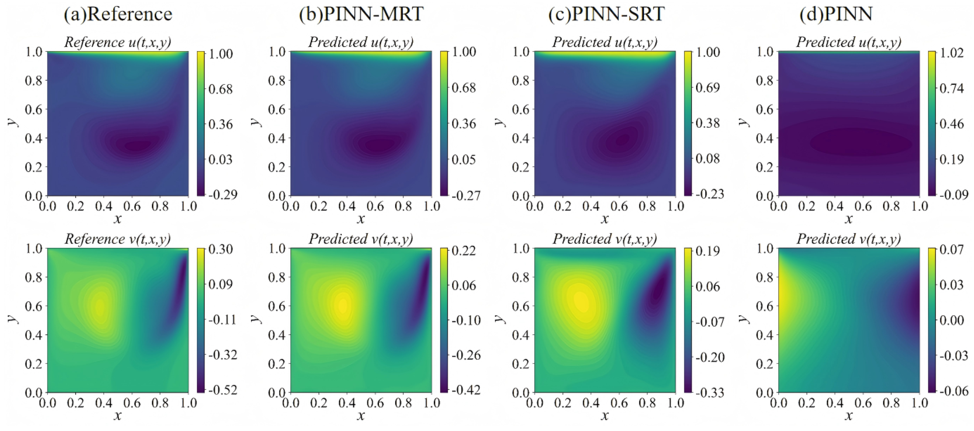
Figure 6.
Absolute error distributions of the velocity components u and v at Re = 1000.
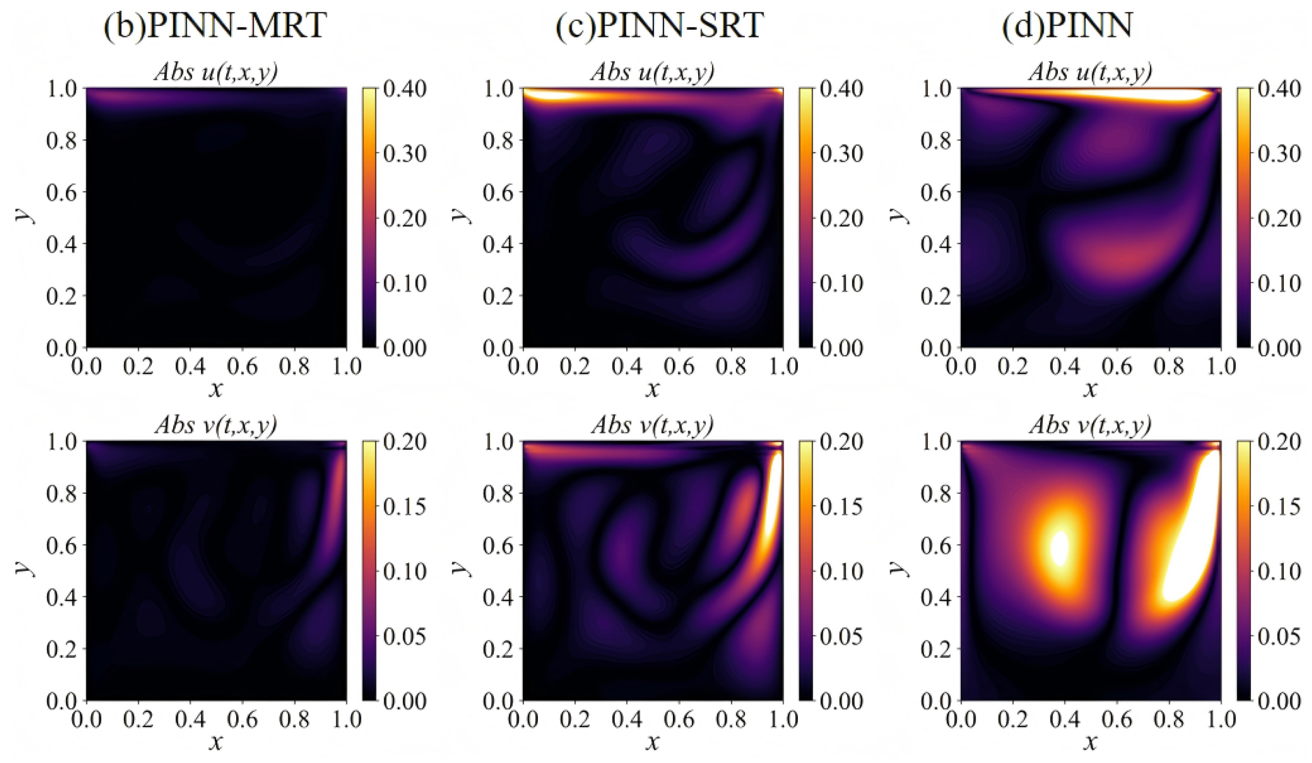
Figure 7.
Relative errors of the inferred parameters (top) and (bottom) under different Reynolds numbers. The left column compares the inversion accuracy of PINN, PINN-SRT, and PINN-MRT models, while the right column shows the robustness of PINN-MRT under noisy data. The shaded areas indicate uncertainty bands.
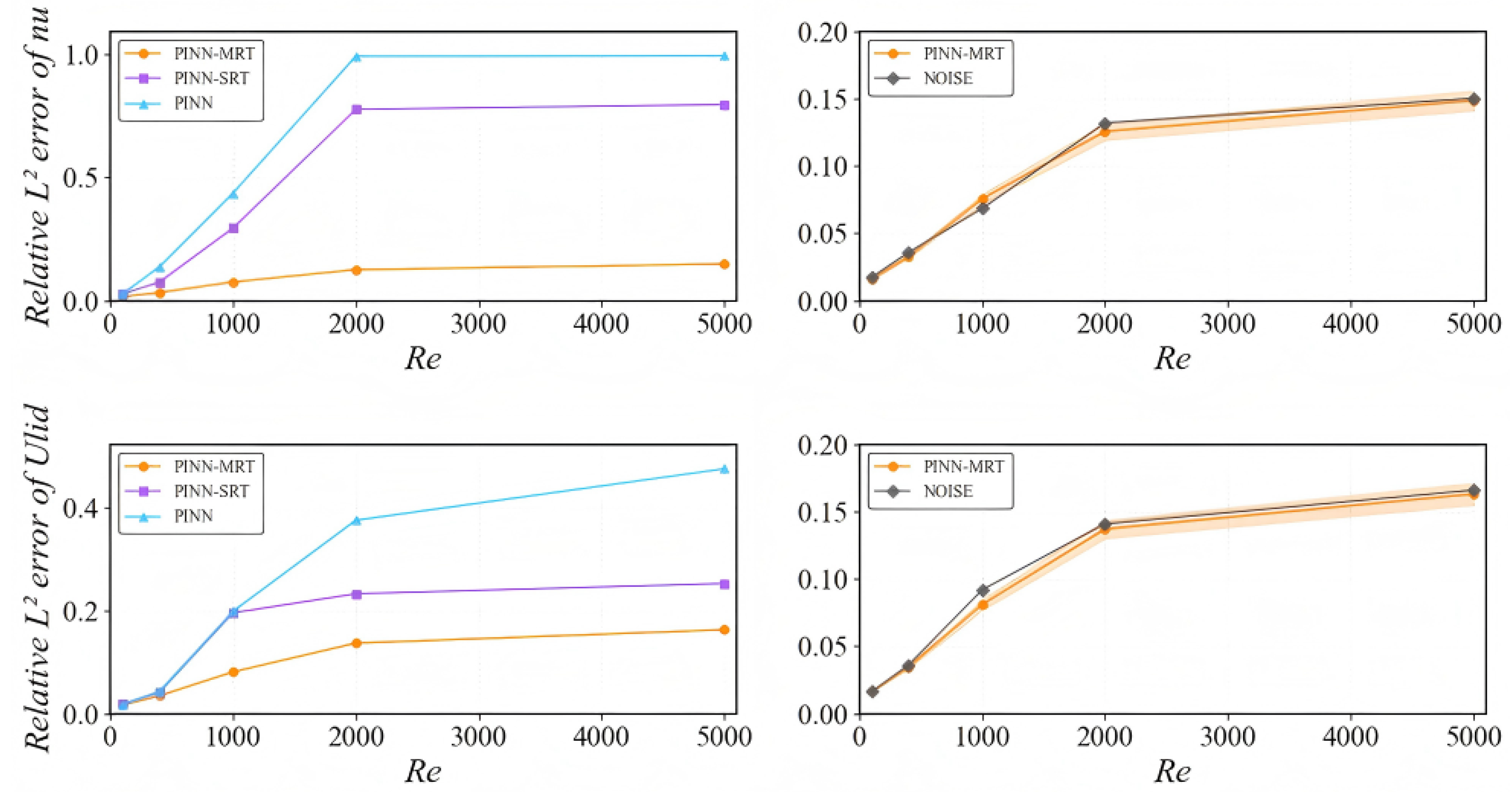
Figure 8.
Forward problem solution comparison of velocity field at Re = 100.
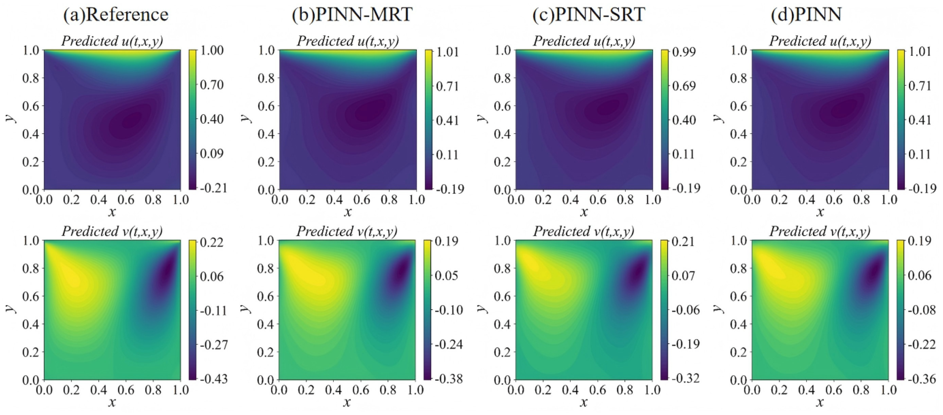
Figure 9.
Absolute error distributions of the velocity components u and v at Re = 100.
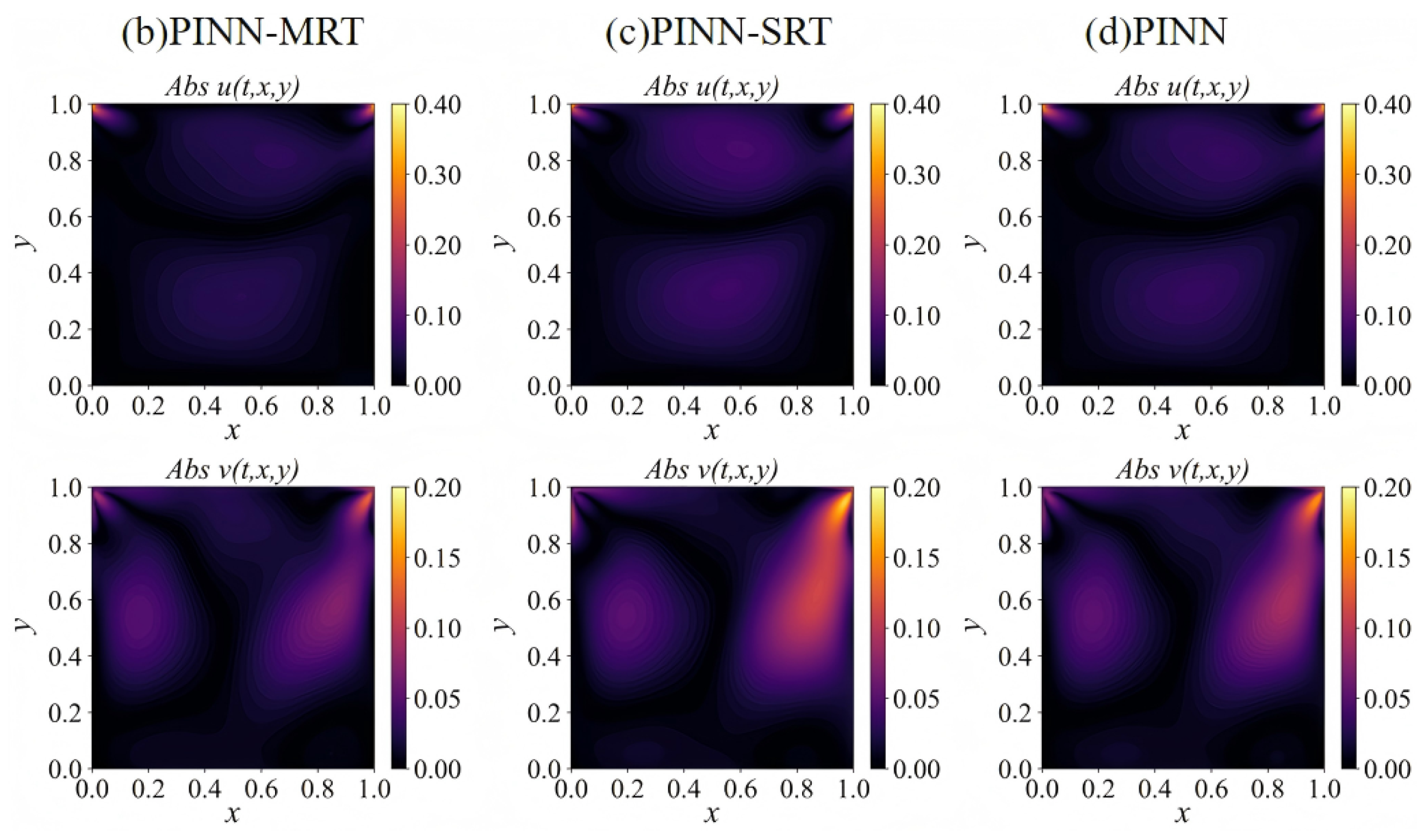
Figure 10.
Forward problem solution comparison of velocity field at Re = 400.
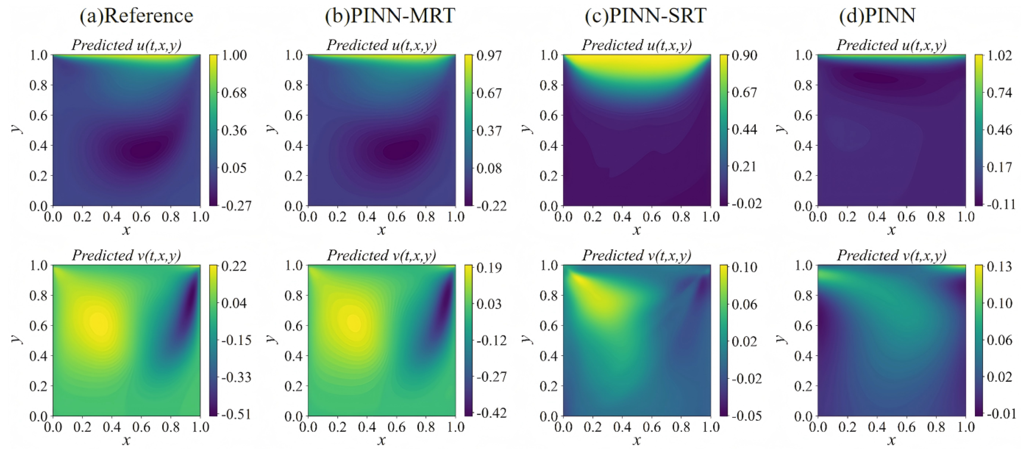
Figure 11.
Absolute error distributions of the velocity components u and v at Re = 400.
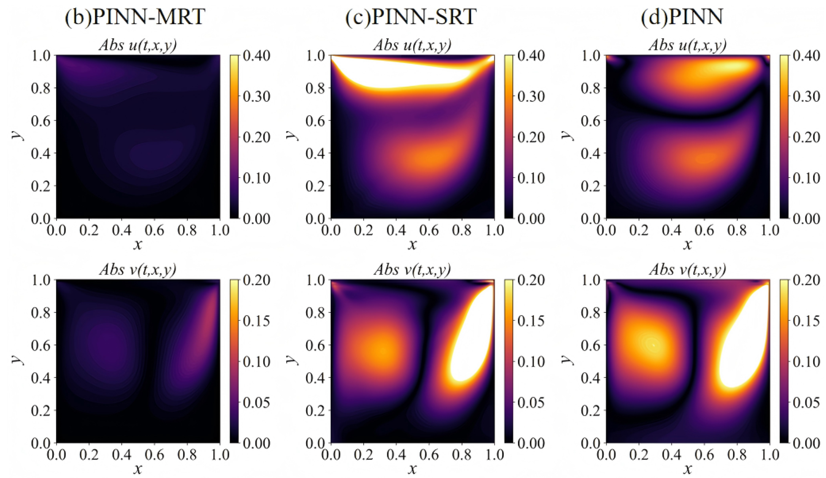
Figure 12.
Relative errors of reconstructed velocity components under kinematic viscosity perturbations from to for different Reynolds numbers. The shaded regions denote uncertainty bands, representing the error tolerance range of the PINN-MRT model.
Figure 12.
Relative errors of reconstructed velocity components under kinematic viscosity perturbations from to for different Reynolds numbers. The shaded regions denote uncertainty bands, representing the error tolerance range of the PINN-MRT model.
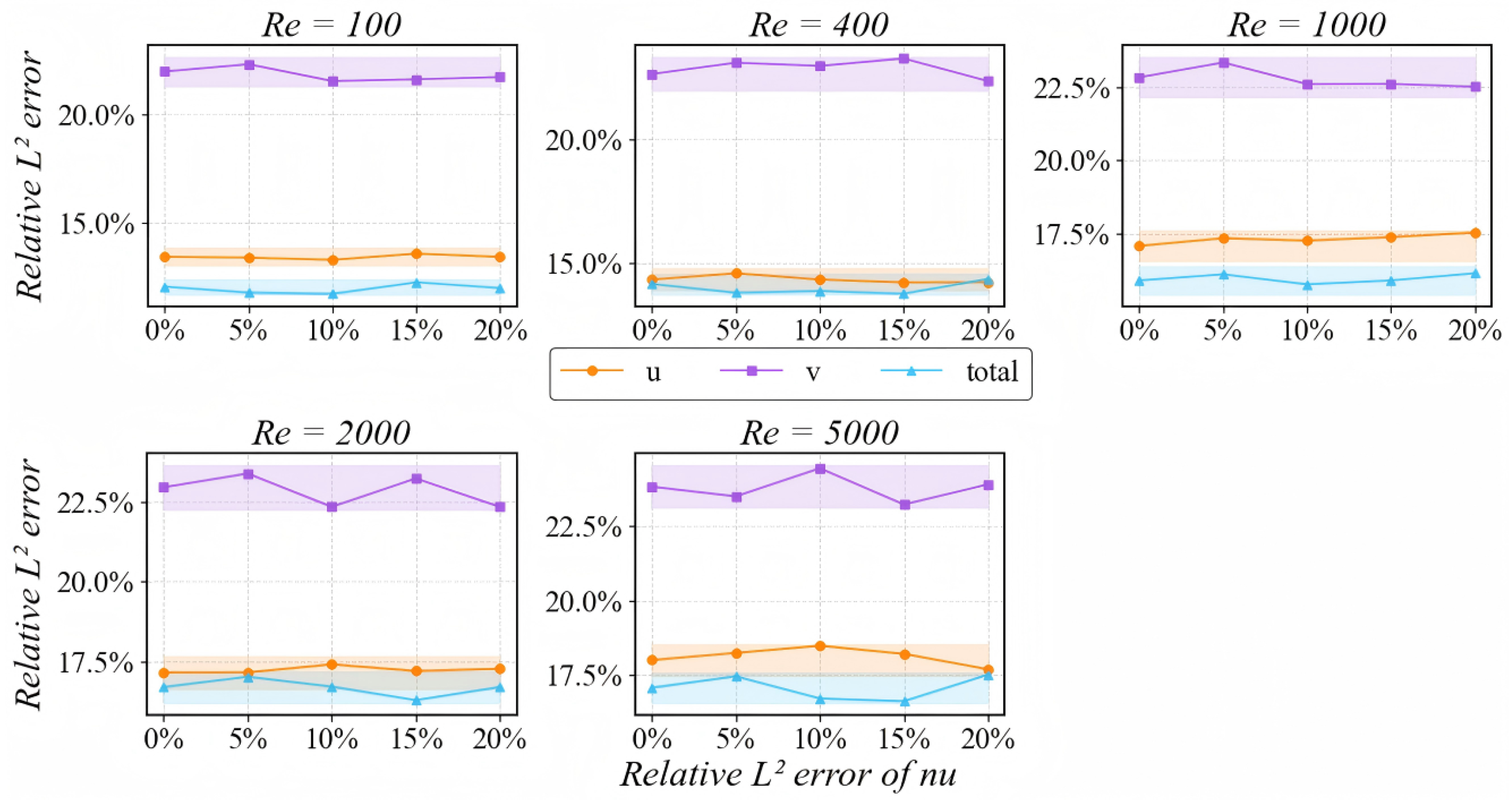

Table 1.
Configurations and training settings for inverse problem.
| Category | Description |
|---|---|
| Network structure | 5-layer fully connected network (1 input, 3 hidden, 1 output) |
| Hidden neurons | 60 neurons per hidden layer |
| Activation function | Tanh |
| Trainable parameter | Both and are randomly initialized in |
| Loss function | |
| Data source | FDM |
| Data location | Random sampling |
| Sampling distribution | 20,000 collocation pts; 5,000 boundary pts; 1,000 data pts |
| Optimizer | Adam (80,000 iterations, initial LR , exponential decay) |
Table 2.
Configurations and training settings for forward problem.
| Category | Description |
|---|---|
| Network structure | 7-layer fully connected network (1 input, 5 hidden, 1 output) |
| Hidden neurons | 60 neurons per hidden layer in ; 100 in |
| Activation function | Tanh |
| Trainable parameter | None |
| Loss function | |
| Data source | None |
| Data location | None |
| Sampling distribution | 20,000 collocation pts; 5,000 boundary pts |
| Optimizer | Adam (80,000 iterations, initial LR , exponential decay) |
Table 3.
Absolute error ranges of horizontal () and vertical () velocity components for all three models in inverse problem at Re = 100 and 1000.
Table 3.
Absolute error ranges of horizontal () and vertical () velocity components for all three models in inverse problem at Re = 100 and 1000.
| Model | ||
|---|---|---|
| Re = 100 | ||
| PINN | [0.0005, 0.0763] | [0.0005, 0.0654] |
| PINN-SRT | [0.0002, 0.0531] | [0.0003, 0.0526] |
| PINN-MRT | [0.0003, 0.0447] | [0.0004, 0.0310] |
| Re = 1000 | ||
| PINN | – | – |
| PINN-SRT | [0.0005, 0.2195] | [0.0001, 0.1318] |
| PINN-MRT | [0.0005, 0.0573] | [0.0001, 0.0635] |
Table 4.
Relative errors (%) of PINN-MRT in inverse problem.
| PINN-MRT | (%) | (%) | (%) |
|---|---|---|---|
| Re = 100 | 9.067 | 11.942 | 4.549 |
| Re = 1000 | 12.179 | 17.048 | 9.894 |
| Re = 2000 | 14.088 | 20.369 | 13.845 |
| Re = 5000 | 15.281 | 21.262 | 14.121 |
Table 5.
Absolute error ranges of horizontal () and vertical () velocity components for all three models in forward problem at Re = 100 and 400.
Table 5.
Absolute error ranges of horizontal () and vertical () velocity components for all three models in forward problem at Re = 100 and 400.
| Model | ||
|---|---|---|
| Re = 100 | ||
| PINN | [0.0001, 0.0765] | [0.0000, 0.0248] |
| PINN-SRT | [0.0004, 0.0851] | [0.0005, 0.1050] |
| PINN-MRT | [0.0003, 0.0447] | [0.0004, 0.0310] |
| Re = 400 | ||
| PINN | [0.0002, 0.3099] | [0.0059, 0.3688] |
| PINN-SRT | [0.0041, 0.5389] | [0.0003, 0.3197] |
| PINN-MRT | [0.0003, 0.1114] | [0.0004, 0.0508] |
Table 6.
Relative errors (%) of PINN-MRT in forward problems.
| PINN-MRT | (%) | (%) | (%) |
|---|---|---|---|
| Re = 100 | 13.436 | 22.014 | 12.058 |
| Re = 400 | 14.328 | 22.669 | 14.145 |
| Re = 1000 | 17.086 | 22.834 | 15.910 |
| Re = 2000 | 17.152 | 22.962 | 16.691 |
| Re = 5000 | 18.003 | 23.815 | 17.076 |
Disclaimer/Publisher’s Note: The statements, opinions and data contained in all publications are solely those of the individual author(s) and contributor(s) and not of MDPI and/or the editor(s). MDPI and/or the editor(s) disclaim responsibility for any injury to people or property resulting from any ideas, methods, instructions or products referred to in the content. |
© 2025 by the authors. Licensee MDPI, Basel, Switzerland. This article is an open access article distributed under the terms and conditions of the Creative Commons Attribution (CC BY) license (http://creativecommons.org/licenses/by/4.0/).
Copyright: This open access article is published under a Creative Commons CC BY 4.0 license, which permit the free download, distribution, and reuse, provided that the author and preprint are cited in any reuse.


