
Submitted:
24 March 2025
Posted:
25 March 2025
You are already at the latest version
Abstract
We used an optomechanical microphone to measure the acoustic signals emitted by compressed-air jets emanating from apertures as small as ~ 5 um. In keeping with the predictions of aeroacoustic theory, spectra extending into the high-frequency (MHz) ultrasound region were observed. Most of this acoustic energy lies well above the range of a conventional ultrasonic microphone. Conversely, the broadband response of the optomechanical sensor offers the potential to localize and quantify leaks based on a more complete knowledge of the acoustic spectrum. We show that the minimum detectable flow rate, set by the onset of turbulence, scales with the hole size and was as low as ~ 10^-3 Pa·m^3·s^-1 for the smallest holes studied here. The results demonstrate that a sufficiently broadband and sensitive microphone might enhance the utility of ‘acoustic sniffer’ tools for quantitative gas leak detection.
Keywords:
micro-scale gas leak detection
; aeroacoustics
; turbulent jet noise
; optomechanical ultrasound sensor
; air-coupled ultrasound
; broadband acoustic sensing
; leak localization
; ultrasonic leak detection
; compressed air diagnostics
; acoustic emissions
I. Introduction and Background
The detection of gas leaks [1,2,3] is a widely studied problem in energy distribution, refrigeration, compressed-air, and vacuum systems [4,5,6,7,8,9,10], and in the certification of sealed structures for the packaging, automotive, and aerospace industries [11,12,13,14,15,16,17,18]. In many cases, reliable identification of leaks, either during manufacture or after deployment, is critically important to both the safety and efficiency of these systems [1,6,7,8,17].
At the highest level, detection methods can be classified [2,3] according to whether their primary utility is for pinpointing the location or quantifying the size of a given leak. These are sometimes delineated as ‘point source’ versus ‘systemic’ methods [10]. Both types have important use-cases, and in fact some techniques are capable of determining, within certain limits, both the location and the size of a leak.
The size of a leak is characterized by its ‘leak rate’, qL = Δ(P·V)/Δt (e.g., with S.I. units of Pa m3 s-1) [1], which essentially predicts the loss (or gain) of pressure per unit time in a fixed volume. Quantitative methods are often compared on the basis of their minimum detectable leak rate, qL,min. Systemic tracer-gas (typically helium) techniques that use mass spectrometry are the gold standard, and can detect leak rates as small as ~10-12 Pa m3 s-1 when referenced to vacuum [4]. However, these systems are relatively complex and costly. Much simpler pressure-change techniques can achieve sensitivities approaching ~ 10-6 Pa m3 s-1 under optimal conditions [17].
To locate a leak, visual ‘bubble inspection’ tests are commonly employed. While these are somewhat laborious and time-consuming, a skilled technician can locate leaks as small as ~10-4 Pa m3 s-1 [17]. An alternative option is provided by ‘sniffers’ [1], which are variously based on thermal conductivity, electrochemical, or mass-spectrometry sensors, and are able to detect and locate leaks in the ~10-6 - 10-2 Pa m3 s-1 range [4]. However, these devices are often gas-specific and can be challenging to use in closed areas where the target gas accumulates, or in open, windy areas where the target gas is not efficiently collected.
Ultrasonic [2,3] (i.e., aero-acoustic [19,20]) leak detection relies on the airborne acoustic signals emitted by a turbulent gas jet. Its attributes include a passive and non-invasive nature and an ability to sense a leak for any type of gas. However, it is traditionally viewed as a low-sensitivity tool, useful mainly for rapid but strictly qualitative identification and localization of a leak [2,4]. In spite of this, the commercial and industrial use of ultrasonic leak detectors is on the rise, driven in part by advances in the on-board computing and signal processing capabilities of low-cost portable instruments. For example, ‘ultrasonic sniffers’ [21] are sometimes preferred over traditional chemical sniffers for locating leaks in HVAC and refrigeration systems [9].
In order to generate detectable sound, a gas leak must lie in a turbulent flow regime [22], which places a fundamental lower limit (e.g., qL,min ~ 10-4 to 10-3 Pa m3 s-1 [1,4]) on the detectable leak rate. However, the practical limit is often significantly higher (e.g., qL,min ~ 10-1 Pa m3 s-1 [17]), due to the impact of interfering signals in the environment and electrical noise in the ultrasonic microphone. Thus, airborne ultrasound techniques have traditionally been restricted to locating relatively large leaks (i.e., large holes, and at relatively large pressures). This is illustrated by several recent studies [5,6,7,9,13,16,19,20], all of which involved hole sizes in the ~0.1 – 1 mm range and leak rates in the ~ 1 - 10 Pa m3 s-1 range.
Aside from noise, another reason that conventional (i.e., electrical) ultrasonic microphones have low sensitivity is that they capture only a small portion (i.e., the low-frequency ‘tail’) of the acoustic power spectrum emitted by a turbulent gas jet, especially for very small holes. In this study, we used a broadband, optomechanical ultrasound sensor to capture the full-range acoustic emissions and show that this offers potential to extend the use of aeroacoustic methods to the detection of smaller holes and lower leak rates than has traditionally been possible, in addition to providing enhanced quantitative information about the leak.
II. Experimental Overview
The leak artefacts used in our study are nominally circular, laser-machined holes (Lenox Laser, Inc.) with diameters of ~ 5, 10, 20, 50, and 75 μm, formed at the end of ‘barb’-style gas fittings. In the manufacture of these holes, a steel endplate of the fitting, with thickness of ~ 200 μm, is subjected to high-power laser pulses until a hole of desired size is formed at the bottom of a much larger crater. The approximate size and circular shape of the holes was verified using an optical microscope, as shown for example in Figure 1(a) for the ~50 μm hole. Additional images are provided in the Supplementary Material (SM) document. The manufacturer specifies a tolerance of +/- 20% for the 5 μm hole and +/- 10% for the others, as indicated by error bars in several plots below.
The barbs were attached to high-pressure tubing and pressurized using either a conventional air compressor for pressures up to ~ 100 psi, or using an air-rifle compressor (Vevor) for pressures up to ~3000 psi. As shown in Figure 1b,c, the microphone was positioned near the micromachined hole to capture acoustic emissions from the gas jets emanating through the hole.
The optomechanical sensor used to detect air-coupled ultrasound in this work is similar to those we have described in great detail elsewhere [23]. These sensors are monolithic, curved mirror Fabry-Perot resonators with their flexible upper mirror acting as the mechanical resonator (i.e., essentially as a tiny ‘eardrum’), and separated from a bottom mirror by a partially evacuated cavity. As in our recent work [24], the sensor chip used here was mounted in a microphone assembly attached to an optical fiber for laser-based readout of the mechanical motion. The particular sensor used to obtain the results below has its first mechanical resonance at ~ 3.7 MHz, and provides a nearly frequency independent noise-equivalent-pressure (NEP) of ~ 50 μPa Hz-1/2 over the entire ~ 20 kHz to 6 MHz range of interest here. Additional details on the experimental setup, the laser-machined barbs, and the sensor (including its calibration for ultrasound measurement) are provided in the SM document.
III. Theory
A. Flow Predictions
In our experiments, the barb fittings are pressurized to some initial value and air escapes through the machined hole into the external, atmospheric-pressure, lab environment. The choice of an appropriate flow model [18] depends on the exact shape (i.e., cylindrical versus tapered, etc.), depth (i.e., length-to-diameter aspect ratio, L/D), and sidewall roughness of the orifice, and some of these details are not completely known here. Nevertheless, the experimental results below are in good agreement with theoretical predictions based on a few reasonable approximations, as follows. First, we assume that the barbs can be modeled as circular holes in ‘thin’ plates (i.e., having small L/D). Second, we assume that the gas flow lies in a continuum regime, characterized by a low value of the Knudsen number (i.e., Kn = λ/d < 0.01, where λ is the mean free path of a gas molecule [10]). These assumptions, which correspond to a ‘compressible flow’ regime [18], are only approximately correct for the smallest holes studied. In fact, those holes are likely to exhibit ‘pipe-like’ flow characteristics (i.e., since L > D is likely) and also lie in a regime intermediate between continuum and molecular flow [10,18]. A compressible flow model is expected to slightly overestimate the flow rates for these small holes [18]. Additional discussion is provided in the SM file.
The compressible flow model is further simplified by assuming isentropic and ‘choked flow’ conditions [11,12]. For air, choked flow requires P1 > 1.89·P0, where P1 is the pressure inside the leaking part and P0 is the external atmospheric pressure; i.e., P0 ~ 101 kPa ~ 14.7 psi. Thus, choked flow conditions correspond to absolute pressures greater than P1min ~ 192 kPa ~ 27.8. psi, or equivalently gauge pressures greater than P1min,G ~ 91 kPa ~ 13.2 psi, well-satisfied by our experimental conditions below. Accordingly, the mass-flow rate (kg/s) can be estimated as [18,19]:
where A is the (effective) orifice area, ψ0 ~ 0.685 for air (see the SM file), Cd is a discharge coefficient which depends on factors such as the shape and roughness of the orifice (but typically Cd ~ 0.8 [10,18,25]), R ~ 287.05 J kg-1 K-1 is the specific gas constant for air, and T ~ 293 K is the temperature, assumed to be the same inside and outside the pressurized object. The leak rate is defined as qL = Δ(P·V)/Δt = Δm(R·T)/Δt, and thus qL = mF·R·T [1,16].
The mass-flow rate can also be expressed as mF = ρ·qV = ρ·v·A, where qV = v·A is the volume flow rate (m3/s) and v is flow velocity, assumed to be the local speed of sound (i.e., v = c) under choked flow conditions. Furthermore, if A is assumed to be the physical area of the orifice then ρ is an effective gas density. From these relationships and using Eq. (1), it follows that ρ ~ P1. In other words, the effective gas density in the orifice scales with the upstream pressure as would also be expected from the ideal gas law. Furthermore, the Reynold’s number in this situation can be expressed as Re = ρ·v·D/μ, where D is the diameter of the orifice and μ is the dynamic viscosity of the gas. For dry air at T ~ 293 K, c = 343 m·s-1, and μ = 1.825×10⁻⁵ kg·m-1·s-1. Using these in the relationships from above, and assuming for simplicity Cd = 1, yields:
where P1 is in kPa and D is in μm. The onset of turbulence typically occurs for some minimum value of Re. For example, ‘fully turbulent’ conditions are often defined by Re > 4000 [11,19]. For thin-orifice plates and pipes, however, the earliest onset of turbulence (i.e., vortex generation) occurs for Re ~ 500-1000 [26]. In any case, Eq. (2) predicts an inverse relationship between the orifice diameter and the pressure required to generate turbulent flow and thus acoustic energy; i.e., P1,min ~ Remin/D. For the choked flow assumptions above, it follows that mF,min ~ Remin·D. This interesting result is well supported by the experimental results below, and implies that the flow rate required to produce turbulent flow conditions (and thus acoustic energy) scales downwards with decreasing hole size.
B. Aeroacoustic Predictions
We next consider the nature of the acoustic power spectrum emitted by the turbulent gas jets described above. It is generally understood that the sources of acoustical energy are vortices and eddies within the turbulent flow. Starting from this point of view, Lighthill [27] derived expressions predicting that the total emitted acoustic power scales as W ~ D2·v8, which is sometimes called the ‘eight-power-velocity’ law [20]. Dah-You reformulated this law in terms of pressure differential, and generalized it to encompass both non-choked and choked flow conditions [28]:
where K ≈ 3×10⁻⁵ is the so-called Lighthill constant. When P1 >> P0, as is typically the case here, Eq. (3) predicts that the acoustic power scales approximately with the square of the aperture diameter and with the square of the internal pressure.
This acoustic power is distributed over a wide frequency range; i.e., it has the form of a ‘turbulent noise’ spectrum, with spectral power increasing as ~ f 2 at low frequencies, reaching a broad peak, and then decreasing as ~ f -2 at higher frequencies [29]. This approximate behavior is captured by a simplified empirical model [28,29]: SW(f) = 4·SW(fp)/(x+1/x)2, where x = f/fp and fp is the frequency of the peak power spectral density (SW). However, it is also known that the shape of the spectrum depends on the observation point relative to the axis of the jet [29]. This has recently [30,31] been attributed to the existence of turbulent structures at two different spatial scales, each having a unique acoustic radiation pattern. For observation points which are normal to or upstream from the gas jet orifice, the so-called fine-scale-structure (FSS or ‘G’) spectrum is typically observed. For observation points in the downstream direction and within a certain cone of angles relative to jet axis, the so-called large-scale-structure (LSS or ‘F’) spectrum is typically observed. In our experiments, the micromachined hole (i.e., the location of the dominant noise sources) is recessed within the barb, and the optomechanical microphone was in all cases located in the downstream direction and at a relatively low angle with the jet axis. Consistent with this, our observed spectra below fit well to the F spectral shape [31]. Additional discussion is provided in the SM file.
Finally, the peak frequency is expected to scale according to a Strouhal relationship [26], fP ~ St·v/D, where St is the Strouhal number, which is approximately fixed over a wide range of Re numbers in a typical system. While St ~ 0.25 is commonly reported for large-scale turbulent jets, a smaller value of St ~ 0.2 was observed for mm-scale jets [28]. We recently observed still smaller values, St ~ 0.1, for air jets emanating from sub-mm needles [32]. Of course, this scaling relationship depends on the ‘critical dimension’ used, and the apparent reduction in St for smaller orifice diameters might be related to boundary effects on the flowing gas [8,10,25,26].
IV. Experimental Results
We first studied the acoustic spectra for each of 5 available hole sizes (~ 5, 10, 20, 50, and 75 μm hole diameters), with the internal pressure set to ~ 1000 psi and a hole-to-microphone distance on the order of ~ 1 cm. For each experiment, this spacing was measured with ~ 1 mm precision and was subsequently used to produce an ‘attenuation-corrected’ plot as explained below. As mentioned above, the manufacturer specifies tolerances on the hole diameter, and this uncertainty is indicated through the inclusion of error bars on several of the plots below. Figure 2(a) shows results for the ~ 75 μm hole, where the red dotted curve is the raw (but calibrated, as explained in the SM document) data reported by the optomechanical microphone. The blue curve is the same measurement, but with the data adjusted on a point-by-point basis to remove the frequency-dependent attenuation of ultrasound by absorption or scattering in air. To estimate this attenuation, we used the simple empirical formula [33] α = 1.6 × 10⁻¹² f [2], where f is the acoustic frequency and α is in units of dB/cm. For example, at 1 cm source-microphone spacing this implies an attenuation of acoustic pressure by a factor of ~ 2× at 2 MHz, ~ 5× at 3 MHz, ~20× at 4 MHz, and ~ 100× at 5 MHz. At MHz frequencies, air-absorption clearly dominates over other sources of attenuation, such as that due to diffraction of spherical waves. Moreover, this rapid scaling of the attenuation is the reason that most air-coupled ultrasound applications are traditionally restricted to frequencies below ~ 2 MHz.
With the frequency-dependent attenuation removed, the adjusted experimental data could be fit very well to the LSS/F spectrum expected for downstream observation points [30,31]. This was true for all 5 hole sizes studied. The analogous case for the~ 10 μm hole is shown in Figure 2(b), and typical fits for the 5, 20, and 50 μm holes can be found in the SM document. From these fits, the peak of each frequency spectrum was estimated and this data was compared against a Strouhal-relationship scaling curve as shown in Figure 2(c). For the two largest holes, it was possible to extract the peak frequency with relatively high confidence, and these data points suggested a value of St ~ 0.14. For the 3 smaller holes, much of the spectrum lies above the practical range (i.e., considering air absorption) of the optomechanical sensor, making the estimation of the peak frequency more prone to fitting error. Nevertheless, these fits suggested St ~ 0.1, which is also reasonable given the discussion in Section III.B and elsewhere [11,16].
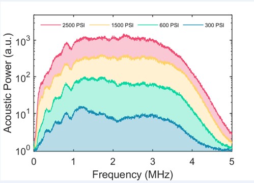
We next consider the variation of the acoustic spectrum and power with internal static pressure for the ~ 5 μm diameter hole. Raw spectra are plotted for various internal pressures (P1) in Figure 3(a), and the acoustic power (~ square of acoustic pressure) at an arbitrarily chosen frequency of 2 MHz is plotted versus internal pressure of the barb fitting in Figure 3(b). This data was collected with ~ 1 cm hole-to-microphone spacing and with the microphone oriented in the downstream direction (i.e., nearly head-on, see Figure 1). As above, acoustic power spanning the entire ~ 0 – 5 MHz range is measured at close spacing. In keeping with the discussion in Section III.B and assuming choked flow conditions at all internal pressures, Figure 3(b) verifies that the acoustic power scales approximately with the square of internal pressure for fixed hole diameter. Small deviations from this scaling are likely attributable in part to a large uncertainty in the internal pressure, which was estimated from the analog gauge built into the compressor.
Given the significant impact of air absorption above ~ 2 MHz, it is interesting to consider the dependence of the received aeroacosutical signals on the hole-to-microphone spacing. For this experiment, the ~ 5 μm diameter hole was pressurized to ~ 1000 psi, the optomechanical sensor and a commercial ultrasonic microphone (Dodotronic Ultramic 384KBLE [34]) were sequentially oriented head-on to the hole, and spectra were collected at various distances. The impact of air absorption is clearly seen in the spectra recorded by the optomechanical sensor shown in Figure 4(a). As distance is increased, the portion of the aeroacoustic spectrum lying above the sensor’s noise floor (~ 50 μPa/Hz1/2) shifts progressively downwards. Nevertheless, even at ~ 10 cm distance there is content extending beyond ~ 1 MHz and the peak received energy is above ~ 0.5 MHz.
The commercial microphone has a bandwidth in the ~ 0 – 192 kHz range, and is constructed around a MEMS sensor (Knowles FG-23629 [35]). Since the microphone manufacturer provides limited specifications regarding noise and sensitivity, we used the self-noise specified by Knowles (NEP ~ 5 μPa/Hz1/2 [35]) to scale the spectra in this case, and also made an assumption that the microphone is operating near the mechanical-thermal noise limit [36]. Regardless of the accuracy of this calibration, the data in Figure 4(b) illustrate a few interesting points. First, the commercial microphone is also able to detect the sound emitted by this small leak, which is not surprising given that its noise floor is likely somewhat lower than that of the optomechanical sensor used. However, the SNR is limited by the low spectral content of the aeroacoustic spectrum in the range of the electrical microphone. Moreover, the bandwidth of the electrical microphone greatly limits the amount of information that can be extracted from the shape of the received spectrum, in contrast with the optomechanical sensor results shown in Figure 4(a). Consistent with this, most commercial ultrasonic leak detectors simply rely on sound pressure level in a narrow frequency range (often near ~ 40 kHz) to identify a leak. Proposals for characterizing a leak based on such narrowband measurements exist, but require prior knowledge about the location of the hole [20] or an ability to vary the internal static pressure of the system [11]. The more complete picture provided by the optomechanical sensor invokes the possibility of an intelligent ‘sniffer’, which could be guided towards a leak by either a human operator or a robot, and might enable a characterization of the leak rate and hole size and shape based on fusing the data collected at various distances.
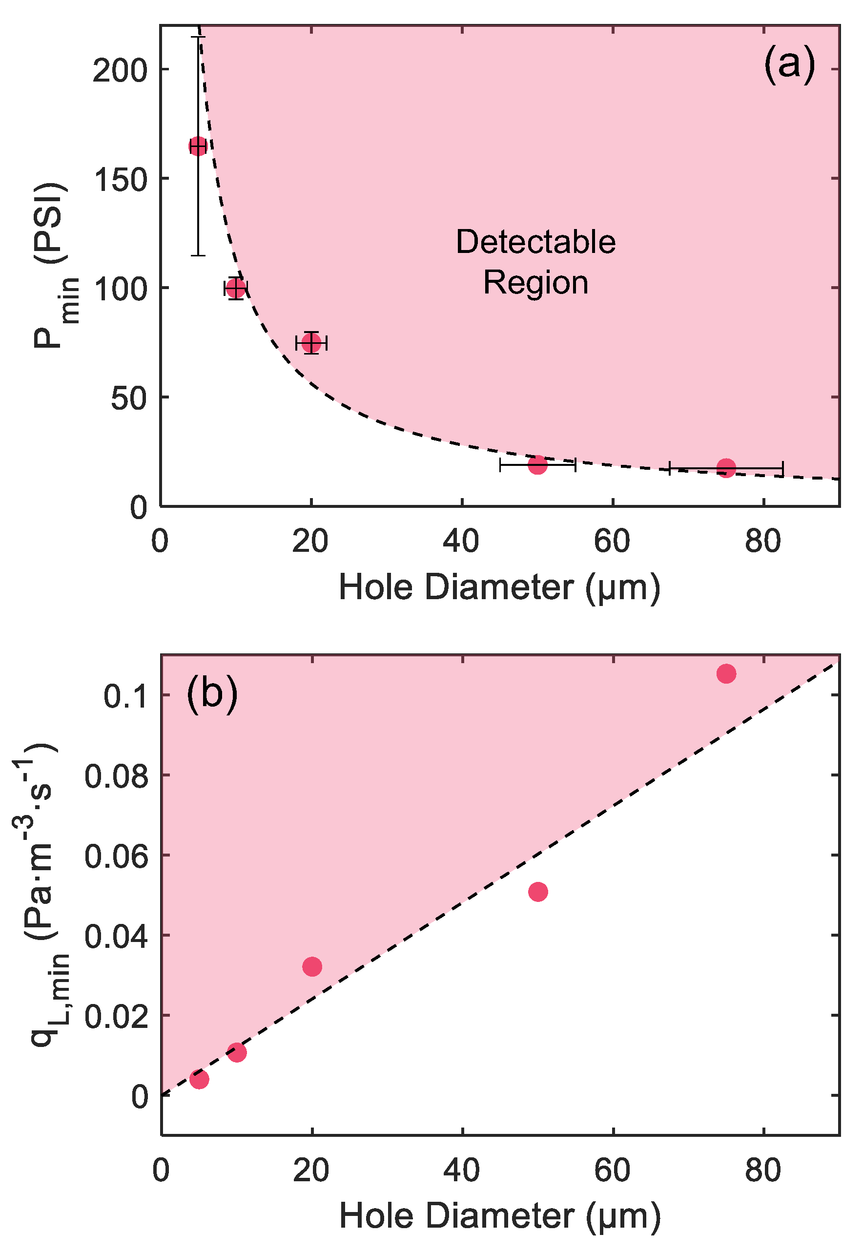
Finally, we considered the minimum internal pressure required to produce measurable acoustic signals for each of the 5 hole sizes studied. For this experiment, the microphone was placed in a nearly head-on orientation and at ~ 1 cm hole-to-microphone spacing. As shown in Figure 5(a), the experimental results are in good agreement with the predictions of the basic flow model outlined in Section III.A, and furthermore assuming a minimum Reynolds number Remin = 1000 for the onset of turbulent flow. While the results shown are for the optomechanical sensor, similar results were obtained using the commercial microphone described above. This supports the conclusion that it is the onset of turbulence, rather than other details such as the microphone self-noise, which determines the minimum detectable flow.
These same results are re-plotted in Figure 5(b), but in this case in terms of the estimated minimum leak rate to produce measurable sound. The predicted minimum leak rate for the largest hole (> 0.1 Pa m3 s-1) is entirely consistent with experimental results for similar and larger hole sizes in the literature [5,6,7,9,13,16,19,20]. In keeping with the discussion in Section III.B, this minimum leak rate scales downwards in proportion to hole size and approaches ~ 10-3 Pa m3 s-1 for the smallest hole. This is consistent with the minimum (i.e., ‘in principle’) detectable leak rate for aeroacoustic detection that have been stated in some sources [3,4,17], but typically without a complete theoretical justification. The wide bandwidth of the optomechanical sensor used here enables a more complete understanding of these limits.
Some caveats should be added with respect to these estimated minimum leak rates. First, our estimates are based on conservative assumptions regarding the appropriate flow model as discussed in Section III.A and also in the SM document. Second, the results shown were obtained using relatively smooth, round holes, which are likely not the most efficient types of orifices for generating turbulence and thus sound. Real leaks are often shaped more like cracks [8] or slits [10] with rough and sharp edges, and it is possible that those orifices would generate turbulence at lower flow rates. Finally, methods for creating sound from laminar jets are known, such as by combining the bubble technique with aeroacoustic detection 6, or by arranging the jetting gas to be incident on some sort of ‘flow mixer’. In light of this, it seems likely that the minimum leak rates estimated from the inherent onset of turbulent flow do not represent an ultimate limit. Using a combined approach, it seems possible that a sufficiently broadband and sensitive microphone might be capable of detecting leak rates well below 103 Pa m3 s-1, which would be competitive with chemical and mass spectrometry sniffers. These admittedly speculative points are left for future study.
V. Summary and Conclusions
Using an optomechanical microphone, we have reported on the acoustic emissions of gas jets emanating from orifices as small as ~ 5 μm. To our knowledge, this is the first report of the aeroacoustic, turbulent jet noise spectra for such small orifices. The results were enabled by the high sensitivity and bandwidth of the optomechanical sensor used. The experimental results, such as the dependence of the acoustic intensity and spectrum on the hole size and static pressure differential, show good agreement with predictions for compressible flow and aeroacoustic sound generation from the literature.
Regarding the aeroacoustic detection of gas leaks, our results help to clarify the minimum leak rates that can be feasibly detected. Importantly, we showed that the minimum leak rate, as determined by the onset of turbulence, scales downward in proportion to hole size. This minimum rate was conservatively estimated to be on the order of ~ 10-3 Pa m3 s-1 for the smallest holes studied here. Moreover, as hole size is reduced, the spectral energy shifts increasingly towards higher frequencies and well beyond the range of conventional (electrical) ultrasonic microphones. However, air absorption at MHz frequencies implies that the detection of such high frequencies is only possible for relatively small hole-to-microphone spacing. In the present study, this distance was on the order of < 10 cm.
Nevertheless, the optomechanical sensor exhibits great potential for use as an ‘acoustic sniffer’ with capabilities beyond that of conventional ultrasonic detectors. Notably, electrical microphones capture only a small portion (the low frequency ‘tail’) of the aeroacoustic spectrum emitted by small leaks, and are thus typically limited to reporting only the relative sound intensity levels. Moreover, the portion of the spectrum that they detect is often polluted by other ultrasonic noise sources in a typical industrial environment. The more complete picture provided by the optomechanical microphone, perhaps combined with machine learning techniques, could enable the detection of smaller leaks, and possibly the quantification of details such as hole size and shape and leak rate, based on the spatial-spectral dependence of the aeroacoustic noise spectrum. We hope to explore these possibilities in future work.
Supplementary Material
The following supporting information can be downloaded at the website of this paper posted on Preprints.org, See supplementary material at [URL will be inserted by AIP] for an extended description of the experimental setup, the optomechanical sensors, and the leak artefacts. This material also provides additional discussion of the flow and aeroacoustic models, as well as supplementary experimental data to support the conclusions in the main text.
Data Availability
The data that support the findings of this study are available from the corresponding author upon reasonable request.
Acknowledgments
This work was supported by NSERC (Discovery Grants Program), The Government of Alberta (Innovation Catalyst Grant), and Emissions Reduction Alberta (Emerging Innovators Challenge).
Conflict of Interest
K.G.S. is an employee at Ultracoustics Technologies Ltd. (I,P), A.C., is an employee at Ultracoustics Technologies Ltd. (I,E). R.G.D. is an employee at North Road Photonics Corp. (I,P) and Ultracoustics Technologies Ltd. (I). G.T. declares no competing interests.
References
- M. Bergoglio and D. Mari, “Leak rate metrology for the society and industry,” Measurement 45, 2434-2440 (2012).
- ASTM E432-91 Standard guide for selection of a leak testing method; American Society for Testing and Materials (2022).
- ASTM E1002-11 Standard practice for leaks using ultrasonics; American Society for Testing and Materials (2022).
- H. Rottlander, W. Umrath, and G. Voss, “Fundamentals of leak detection,” Leybold GmbH White Paper, Cat. No. 199 79 VA_.02, (2016).
- P. Eret and C. Meskell, “Microphone arrays as a leakage detection tool in industrial compressed air systems,” Adv. Acoust. Vibr. 2012, 689379 (2012).
- J. Li, Y. Li, X. Huang, J. Ren, H. Feng, Y. Zhang, and X. Yang, “High-sensitivity gas leak detection sensor based on a compact microphone array,” Measurement 174, 109017 (2021).
- J. C. Lee, Y. R. Choi, and J. W. Cho, “Pipe leakage detection using ultrasonic acoustic signals,” Sens. Actuat: A. Phys. 349, 114061 (2023).
- S. Zhang, G. Chen, Z. Li, and J. Fang, “Computational fluid dynamics analysis of flammable refrigerant leakage through a microcrack,” Int. J. Refrig. 134, 35-44 (2022).
- D. Colbourne and A. L. Vonsild, “Detection of R290 leaks in RACHP equipment using ultrasonic sensors,” Int. J. Refrig. 151, 342-353 (2023).
- I. D. Lee, O. I. Smith, and A. R. Karagozian, “Hydrogen and helium leak rates from micromachined orifices,” AIAA Journal 41(3), 457-464 (2003).
- D. Wang, F. Zhao, and T. Wang, “The ultrasonic characteristics study of weak gas leakage,” 2015 International Conference on Fluid Power and Mechatronics (FPM), Harbin, China, 2015, pp. 681-685. [CrossRef]
- T. Wang, X. Wang, and M. Hong, “Gas leak detection based on data fusion with time difference of arrival and energy decay using an ultrasonic sensor array,” Sensors 18, 2985 (2018).
- P. Holstein, M. Barth, and C. Probst, “Acoustic methods for leak detection and tightness testing,” in 19th World Conference on Non-Destructive Testing, (2016).
- F. Gao, J. Lin, Y. Ge, S. Lu, and Y. Zhang, “A mechanism and method of leak detection for pressure vessel: whether, when, and how,” IEEE Trans. Instrum. Meas. 69(9), 6004-6015 (2020).
- Y. Lyu, M. Jamil, P. Ma, N. He, M. K. Gupta, A. M. Khan, and D. Y. Pimenov, “An ultrasonic-based detection of air-leakage for the unclosed components of aircraft,” Aerospace 8, 55 (2021).
- G. R. Piazzetta, R. C. C. Flesch, and A. L. S. Pacheco, “Leak detection in pressure vessels using ultrasonic techniques,” Proceedings of the ASME 2017 Pressure Vessels and Piping Conference. Waikoloa, Hawaii, USA. July 16–20, 2017. [CrossRef]
- E. Schlick-Hasper, M. Neitsch, and T. Goedecke, “Industrial leak testing of dangerous goods packaging,” Packag. Technol. Sci. 33, 273-286 (2020).
- H. Yoshida, M. Hirata, T. Hara, and Y. Higuchi, “Comparison of measured leak rates and calculation values for sealing packages,” Packag. Technol. Sci. 34, 557-566 (2021).
- E. Naranjo and S. Baliga, “Expanding the use of ultrasonic gas leak detectors: a review of gas release characteristics for adequate detection,” Gases Instrum. 7, 24-29 (2009).
- S. Wang and X. Yao, “Aeroacoustics measurement of the gas leakage rate for single hole,” Rev. Sci. Instrum. 91, 045102 (2020).
- See for example: https://www.uesystems.com/ultrasound-leak-detection/, accessed Feb. 22, 2025.
- A. Powell, “Why do vortices generate sound?,” Transactions of the ASME 117, 252-260 (1995).
- G. J. Hornig, K. G. Scheuer, E. B. Dew, R. Zemp, and R. G. DeCorby, “Ultrasound sensing at thermomechanical limits with optomechanical buckled-dome microcavities,” Opt. Express 30(18), 33083-33096 (2022).
- K. G. Scheuer and R. G. DeCorby, “Air-coupled ultrasound using broadband shock waves from piezoelectric spark igniters,” Appl. Phys. Lett. 125, 082202 (2024).
- R. A. Jackson, “The compressible discharge of air through small thick plate orifices,” Appl. Sci. Res. 13, 241-248 (1964).
- W.K. Blake and A. Powell, “The development of contemporary views of flow-tone generation,” in: Krothapalli A and Smith CA (eds) Recent advances in aeroacoustics. Berlin: Springer, 1986, pp.247–325.
- J. Lighthill, “Some aspects of the aeroacoustics of high-speed jets,” Theoret. Comput. Fluid Dynamics 6, 261-280 (1994).
- M. A. A. Dah-You, “General laws and reduction of aerodynamic noise,” in L. Peizi (Ed.), Proceedings of Inter-noise 87, (1 pp. 21-34). Beijing, China.
- H. S. Ribner, “On spectra and directivity of jet noise,” J. Acoust. Soc. Am. 35, 614-616 (1963).
- C. K. W. Tam, K. Viswanathan, K. K. Ahuja, and J. Panda, “The sources of jet noise: experimental evidence,” J. Fluid Mech. 615, 253-292 (2008).
- T. B. Neilsen, K. L. Gee, A. T. Wall, and M. M. James, “Similarity spectra analysis of high-performance jet aircraft noise,” J. Acoust. Soc. Am. 133, 2116-2125 (2013).
- K. G. Scheuer and R. G. DeCorby, “All-optical, air-coupled ultrasonic detection of low-pressure gas leaks and observation of jet tones in the MHz range,” Sensors 23, 5665 (2023).
- S. Takahashi, “Properties and characteristics of P(VDF/TrFE) transducers manufactured by a solution casting method for use in the MHz-range ultrasound in air,” Ultrasonics 52, 422-426 (2012).
- https://www.dodotronic.com/product/ultramic-384k-ble/, accessed Feb. 22, 2025.
- https://www.knowles.com/series/dpt-hearing-aid-components-accessories/subdpt-hearing-instruments-microphones/series-fg-bfg, accessed Feb. 22, 2025.
- T. B. Gabrielson, “Mechanical-thermal noise in micromachined acoustic and vibration sensors,” IEEE Trans. Electron Dev. 40(5), 903-909 (1993).
Figure 1.
(a) A microscope image (captured with a 2.5× objective lens) of the nominally 50 μm hole, with the hole illuminated from the backside. (b) A schematic showing the experimental setup, with the microphone oriented at 90° relative to a laser machined hole. (c) Alternate configuration used to capture some data, with the microphone oriented at 0° (i.e., ‘head-on’) to the hole.
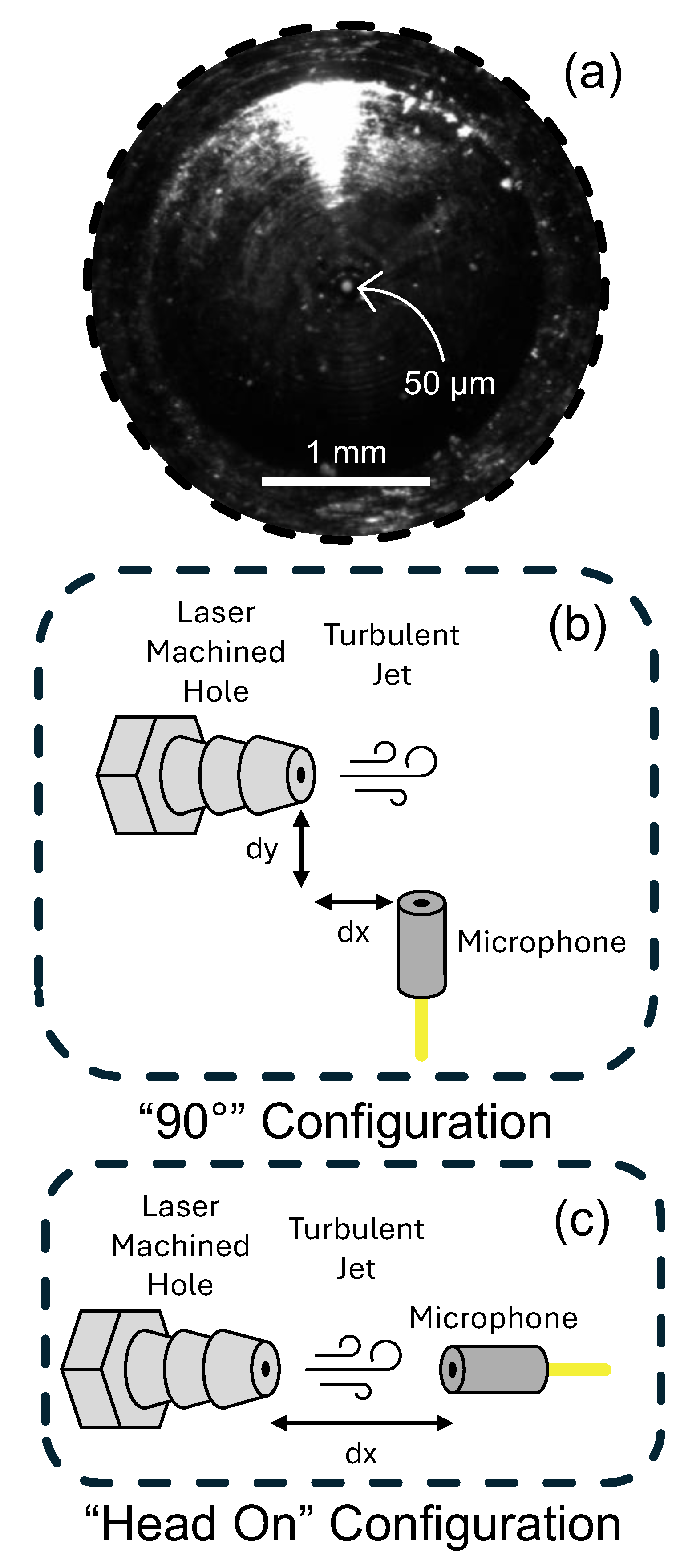
Figure 2.
(a) Typical acoustic frequency spectrum for the ~75 μm diameter hole. The blue-solid curve is the raw spectrum, the red-dotted curve is the experimental data corrected for air attenuation between the hole and the microphone, and the black-dashed curve is a semi-empirical fit using the LSS-spectrum (see main text). (b) As in part a, but for the ~10 μm diameter hole. (c) Typical peak frequencies for each hole diameter (red symbols), estimated from fits of the type shown in parts a and b. The black-dashed and black-dash/dot curves are Strouhal scaling functions for St = 0.14 and 0.1, respectively.
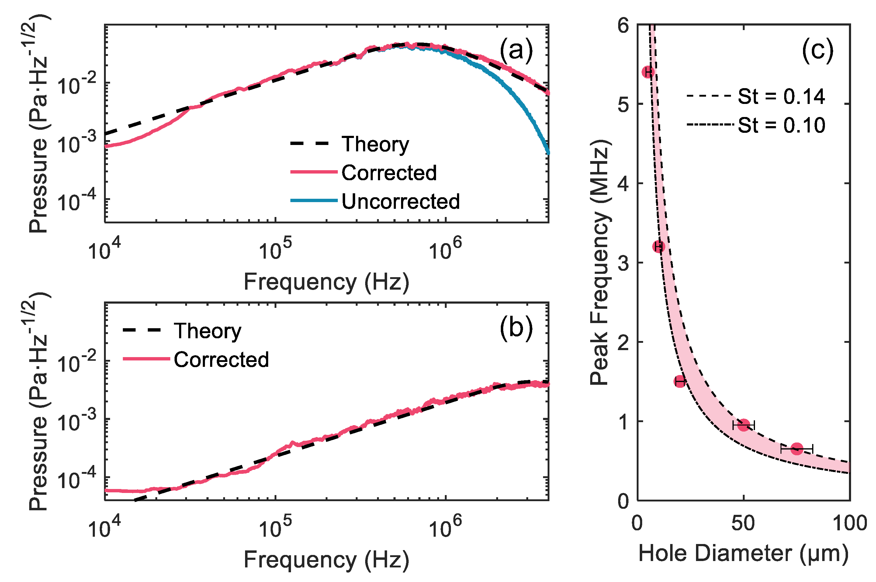
Figure 3.
Acoustic spectra for the ~ 5 μm diameter hole as internal pressure is varied. (a) The raw frequency spectrum (i.e., not corrected for air attenuation) is plotted for various gauge pressures as indicated by the legend. (b) The acoustic power (i.e., ~ P2) at 2 MHz is plotted versus internal absolute pressure. Experimental data points are indicated by the red symbols, while the black dashed line represents a ~ P12 scaling curve as predicted by the Lighthill analogy and assuming choked flow conditions with P1 >> P0.
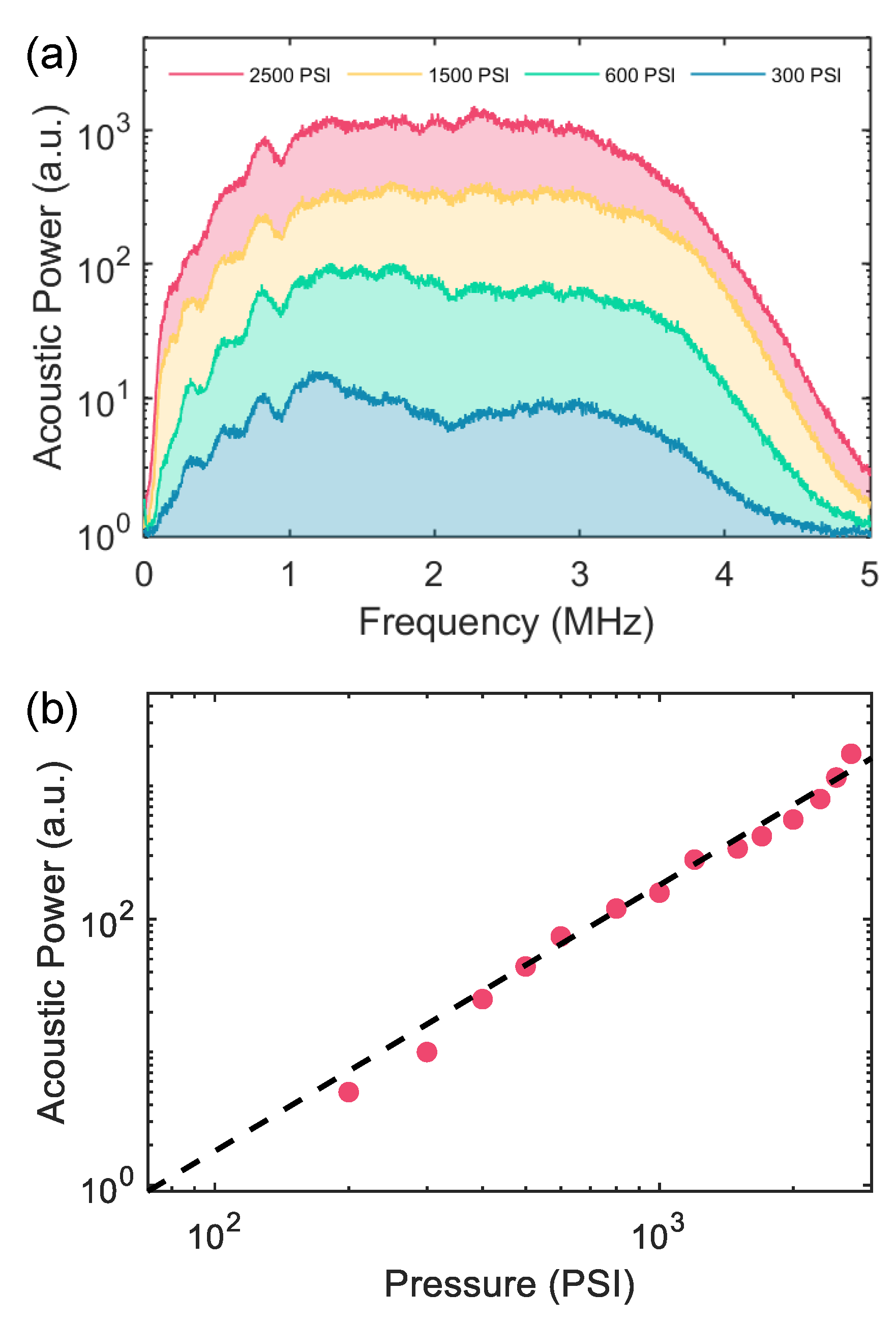
Figure 4.
Acoustic frequency spectrum for the ~ 5 um diameter hole at internal pressure ~ 1000 psi, and with the microphone in a ‘head-on’ orientation. (a) Raw spectra recorded by the optomechanical microphone for various hole-microphone distances as indicated by the legend. (b) Raw spectra recorded by a commercial ultrasonic microphone (see the main text) for various hole-microphone distances as indicated by the legend.
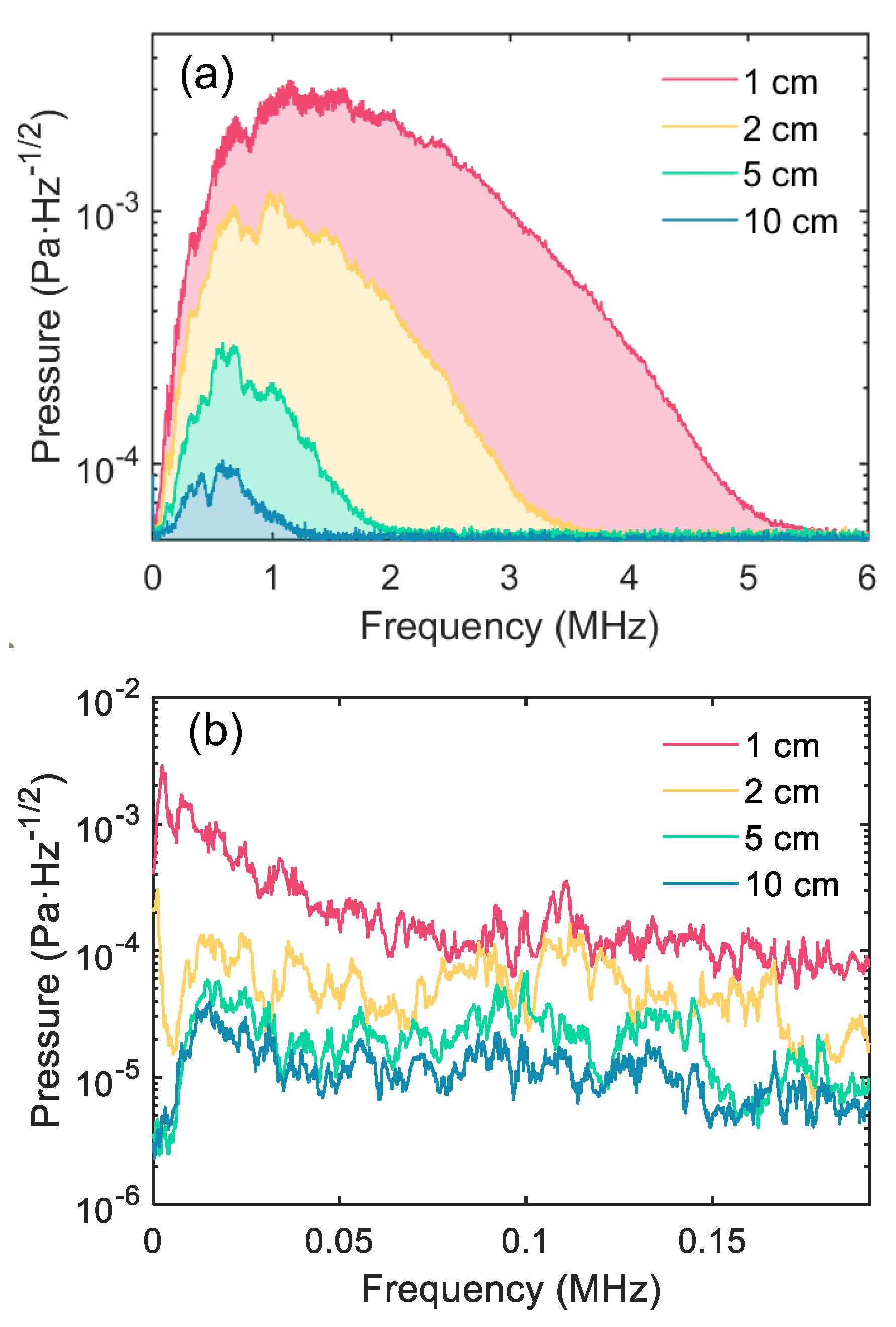
Figure 5.
(a) Minimum absolute internal pressure required to produce measurable acoustic signals using the optomechanical sensor is plotted versus the nominal hole diameter. The red symbols indicate the experimental estimates for ~ 1 cm hole-to-microphone spacing. The black dashed line is the theoretical prediction assuming compressible, choked flow and Remin = 1000 (see main text). (b) Minimum leak rates for ultrasonic detection, as derived from the results in part a. In both, the red shaded areas represent regions where gas leaks generated detectable sound in the present study.
Disclaimer/Publisher’s Note: The statements, opinions and data contained in all publications are solely those of the individual author(s) and contributor(s) and not of MDPI and/or the editor(s). MDPI and/or the editor(s) disclaim responsibility for any injury to people or property resulting from any ideas, methods, instructions or products referred to in the content. |
© 2025 by the authors. Licensee MDPI, Basel, Switzerland. This article is an open access article distributed under the terms and conditions of the Creative Commons Attribution (CC BY) license (http://creativecommons.org/licenses/by/4.0/).
Copyright: This open access article is published under a Creative Commons CC BY 4.0 license, which permit the free download, distribution, and reuse, provided that the author and preprint are cited in any reuse.


