
Submitted:
23 March 2025
Posted:
24 March 2025
You are already at the latest version
Abstract
This paper presents a comprehensive investigation into dead reckoning algorithms. The study begins with an in-depth analysis of the fundamental mathematical formulation for navigation position calculations, then introduces the concept of local invariance to refine traditional methods by examining state parameters with inherent stability. Building on this foundation, we propose an efficient iterative optimization algorithm designed specifically for real-time trajectory prediction under sparse sensor data conditions(Only three samples are required). This approach effectively mitigates the impact of data scarcity, enabling robust and accurate trajectory predictions in challenging environments. The proposed method is anticipated to play a pivotal role in following control systems, thereby significantly improving their operational reliability and performance.
Keywords:
Dead Reckoning Algorithm
; Local Invariance
; Sparse Sensor Data
; Iterative Optimization Algorithm
1. Introduction
Dead reckoning (DR) is a fundamental navigation technique that estimates the position of an object based on its initial position and subsequent velocity or acceleration measurements. DR is particularly valuable in environments where global navigation satellite systems (GNSS) are unavailable or unreliable. For example, in robotics, dead reckoning can help wall-climbing robots navigate using information fusion from multiple sensors [1]. In marine biology, DR has been used to study animal movements, such as tracking marine turtles in controlled environments [2]. For animals, researchers have debated how frequently dead-reckoned paths should be corrected for drift to ensure accuracy [3].
Methodological Advances. Recent advances have combined dead reckoning with other techniques to improve accuracy. For instance, the use of desgined sensor [4] and unscented Kalman filters (UKF) [5] in pedestrian positioning has enhanced DR performance by fusing multi-sensor data effectively . Others have explored artificial intelligence (AI)-enhanced inertial measurement units (IMUs) for dead reckoning, achieving notable results in intelligent vehicles [6]. Research has also focused on improving DR through complex motion mode recognition. For example, Ze et al. developed a hierarchical classification approach for pedestrian dead reckoning under varying movement conditions [7]. Similarly, Dror et al. have explored deep learning techniques to enhance inertial navigation systems (INS), demonstrating how machine learning can optimize DR algorithms in challenging environments [8].
Current Challenges. Despite these advancements, several challenges remain. For one, maintaining accuracy over time without external corrections remains difficult, as errors tend to accumulate. Additionally, the performance of DR heavily depends on sensor quality and data fusion methodologies. As noted by Gunner et al., even modern systems require careful consideration of correction intervals to balance energy consumption and tracking fidelity [3].
Therefore, we analyze the basic form of the dead reckoning algorithm model, especially put forward the concept of local invariance, and improve the dead reckoning method by finding the expected final state parameters with better invariance, and design an efficient optimization iterative algorithm to better cope with the high real-time trajectory prediction scenario under the condition of sparse sampling data.
2. Problem formulation and modeling
DR usually speculates on the state of motion at some point in the future based on the current estimated state of motion . Usually its standard form is Equation (1), where the vector denotes the state of motion, denotes the speed (first derivative of the state of motion), and denotes the acceleration (second derivative of the state of motion).
However, we can find that dead reckoning usually takes certain states or patterns as invariants and continues to speculate on the next state of motion of the moving target. Based on this understanding, we can improve the traditional dead reckoning method and solve the extrapolation problem by introducing new invariants.
2.1. Time-invariance of motion parameters
Specifically, we take an aircraft as an example to explore which parameters are regarded as invariants when extrapolating its motion state. Moreover, we conduct a further analysis of the advantages and disadvantages of such invariants in dead reckoning.
Let be the position vector of the extrapolation reference point in the world coordinate system, be the velocity vector in the body coordinate system, and represent the tangential acceleration. is the skew-symmetric matrix form (Lie algebra) of the angular velocity vector. The corresponding DR algorithm is shown in the Equation (2). Obviously, , , and are the default invariants in dead reckoning algorithms.
Among them, the exponential mapping in Equation (2a) is expanded as follows:
By setting a fixed state synchronization period to correct the dead reckoning error, we can obtain a three-dimensional space track and dead reckoning trajectory as shown in Figure 1. The red trajectory curves is the actual motion path of the aircraft. The continuous yellow line segments are the predicted (extrapolated) trajectories at equal time intervals. The segments where the transition from the yellow to the red trajectories occurs are the hard synchronizations when the error threshold is surpassed.
By projecting the trajectory onto a plane consisting of vertical and x-axis, the Figure 2 can be obtained, and the relationship between the line segments (the blue dashed lines) and the smooth trajectory (the black curves) calculated according to the second-order dead position can be seen. It can be seen that after the imminent large overload maneuver at , the maximum deviation in the vertical direction of dead reckoning reaches . Because the acceleration in the vertical direction is changing rapidly, even in reverse.
Analyze sources of error. Since velocity and acceleration are simply considered as constants during actual motion, when the time span is large, the deviation can easily exceed the allowable range, i.e., the invariance of the selected parameters is poor. Therefore, one way to improve the dead reckoning method can be to select a parameter with better invariance for dead reckoning. In most cases, the higher the order of the motion parameters, the more sensitive to the measurement noise, and the lower the order of the motion parameters, the worse the invariance. And for a controlled object, there is one potential parameter with relatively good time-invariance, and that is the desired end state of motion. When we take the parameter in the control law as a motion parameter with good time-invariance, we may be able to get better dead reckoning results.
2.2. Time-invariant parameters in optimal control
When choosing a class of control laws as a reference, we give preference to the optimal control. Optimal control is common and representative in nature and in practical engineering applications. In practical engineering, in the aerospace field, spacecraft orbit transfer relies on optimal control to determine the optimal thrust direction and magnitude, to minimize fuel consumption and mission time, and is used for spacecraft attitude control. Aircraft flight control uses optimal control to optimize flight trajectory, fuel consumption, and time. We use the following assumptions to standardize the dead reckoning objects discussed next.
Assumption A1.
Moving entities possess the capabilities of route planning and motion control.
Assumption A2.
The moving entity can independently establish the desired target state on its own. However, it will not take the initiative to notify the observing side.
Assumption A3.
The entity adopts optimal control in the motion planning of the flight route (continuous state control). Let the entity state be , the control input be , and the corresponding state equation be . The performance index of the optimal state control is described as follows:
Where and are scalar functions, representing the positive definite expressions of the state error and the input respectively.
To facilitate the analysis and discussion, we simplify the problem to the optimal guidance control in a two-dimensional plane. In Figure 3, the position at time t, namely , is located at the lower left corner. The angle between the moving velocity V and the horizontal axis of the coordinate system is . The azimuth angle is formed by the desired waypoint relative to the current position of the moving entity, and represents the velocity direction constraint when reaching the desired position in the constraints.
Where,
and
Let , , it could be obtain that,
Set , and , thus the state-space expression of the control system can be obtained,
The scalar functions of and in the Equation (3) are designed as matrices of parameters Q and R of quadratic functional functions, and the indicator becomes
To solve the optimal control problem of a second-order system using the Pontryagin’s Minimum Principle, the control law should take the following form,
The optimal guidance law corresponding to the solution of the Riccati equation based on the parameter matrix Q and R should take the following form in Equation (9)
It can be clearly observed that the moving object under optimal guidance control, states , are parameters with stable time-invariant characteristics. However, since Equation (9) is not a convex function, the expected final state cannot be estimated by the least squares method.
2.3. Geometric properties of trajectory
Therefore, we analyze its geometric properties to convert it into a convex function that can be solved. Use a classic math trick, multiply both sides of Equation (9) by and then substitute it into Equation (4), the following equation can be obtained.
Where b and d are respectively,
To simplify the expression in Equation (10), define , and .
The conventional method is to select before t at the current moment to get three Equation (10) by solving a system of nonlinear equations, solving for three unknowns. However the problem is, in fact, it is not possible to obtain a convergent solution by directly applying Newton’s method, L-M solver, etc. (experimental test), and it is necessary to first transform the solution problem into a reasonable optimization problem (preferably a convex optimization problem).
Continue to work on the Equation (10), we can find that for any selection of , there is a parametric circle with the coordinates of the center of the circle where and , and the radius of the circle is , and the circle intersects the trajectory line at and . Literally, if the parameter circle corresponding to a sampling point intersects the trajectory line at the desired endpoint, then the parameter circle corresponding to two different sampling points must intersect at the desired endpoint together. Thus we can generalize its geometric properties as following.
Property 1.
The parameter circles of any sample point on the trajectory line are intersected at the same point.
Property 2.
The same point at which the parametric circles intersect is the desired final state position.
In order to reflect the above properties, we select a trajectory, and select the sampling points at second, second and second, respectively, and plot its parameter circles in Figure 4, which can clearly be seen that each circle intersects with the trajectory line at the sampling point and the desired end point, and the parameter circles pass through a common point .
2.4. Convex function construction
In order to solve for the time-invariant parameter of the desired final state. We construct a convex function using property 1, that parametric circles intersect at the same point.
Firstly, the analytical solution of the intersection of two parameter circles is studied. For two sampling moments and , there are two parameter circles. Suppose, the centers of two circles are at and , and the radius are and , respectively. Thus, the midpoint between two parameter circles is , define L as the distance in between, and take the unit basis vector in the direction from one circle’s center to another, while the orthogonal unit basis vector is . Thus, we can get the analytic solution of the two intersections in Equation (12).
Where,
and
In terms of the form of the analytical solution, there may be no intersections, i.e., imaginary roots, as shown in Figure 5. Therefore, the search space may not be limited to the real domain space , and in order for the algorithm to run robustly, we extended the problem to the unitary space in Section 3.
The process of solving for and is regarded as the optimal estimation of the parameters. Once these values are obtained, they are substituted into Equation (10), which allows us to obtain the set of three parametric circles for with . There are up to 6 intersections between the 3 circles on the plane, and according to the geometry of the problem, 3 of them intersect on the trajectory line at the desired end point of the trajectory. If we take any two parametric circles from them, say those corresponding to indices i and j , there will be two intersection points and , which constitute the geometric properties of the system. It can be observed that there is a probability of selecting the potential common point (end point of the trajactory) from the intersection points provided by each pair of circles. Consequently, there are 8 possible combinations. It is preferable to use binary (where the symbol + represents the positive root and the symbol − represents the negative root) to represent and define the intersection point combinations simultaneously.
However, there is only one combination belong to that can be optimized to obtain the final optimization result. According to property 1, a certain intersection and common point between the parametric circle and the parametric circle, we get the 2-norm corresponding to the first part of the optimization objective function, and according to property 2, the common point is also the desired end point of the trajectory line, we can get the 2-norm corresponding to the second part of the objective function in Equation (14).
Thus, the parameter estimation problem becomes the one shown in Equation (15), which is solved so that the sum of two sqares of the 2-norms is taken as the smallest combination of intersection points and the corresponding target end state and . Obviously, the optimization goal V is positively definite, and if is negatively definite, and the problem model is a convex optimization problem, these would ensures that any local minimum is also a global minimum.
Thus, the optimization problem for parameter estimation takes the form shown in Equation (15). That is, the sum of the distances between the intersections is minimal, and the sum of the distances between the intersections and the final state positions is also minimal. To make the sum of squares of the norm representing the distances equal to 0, two conditions need to be met simultaneously: 1. the selected intersection group is correct; 2. the solution is precisely the corresponding target ending states and .
3. Methods
As mentioned in the previous section, there are a total of 8 possible branches that need to be optimized and iterated to find the final optimal solution, so we propose the Pseudoinverse Gradient Descent Method with Eight Branch Directions (8B-PGDM). Since V is the sum of two sqares of the 2-norms, it is obviously a convex function, assuming that the intersections can be extended to unitary space, then it is not affected by the undefined imaginary intersection point, and the variable can be considered unconstrained, then the optimization objective function V is a convex optimization problem. Since it is a convex optimization problem, common optimization solvers, such as Pseudoinverse Gradient Descent Method can be used to solve the problem.
3.1. Pseudoinverse Gradient Descent Method
Considering that the optimization target V is positively definite, then, as long as the appropriate is taken to make negatively determined, then it can converge asymptotically to 0 according to Lyapunov’s theorem. The existence of the optimal solution is proven. Based on this existence result, we develop a method named Pseudoinverse Gradient Descent Method (PGDM), which leverages the properties of the problem. Specifically, the existence of the optimal solution guarantees that our algorithm has a theoretical target to converge to. Additionally, by exploiting the convergence properties of the solution, we design the update rules, step size adjustment strategies, and termination conditions of PGDM to ensure that it can efficiently find the optimal solution."
Since the dimension of is 3, we need at least 3 linearly independent equations to find the inverse of the relevant matrix in order to solve for these unknowns. To this end, we consider expanding and in terms of the X and Y axes by expressing and as functions of the components on the X and Y axes through projection. Then, by taking derivatives of these functions with respect to , we obtain a system of equations. If the resulting coefficient matrix of this system of equations is not invertible, we can use the Moore-Penrose pseudoinverse to solve for the optimized gradient direction. This is because the pseudoinverse provides a least-squares solution, which is particularly useful when dealing with overdetermined or underdetermined systems of equations.
According to the situation of the current branch, the pseudo-inverse of the Jacobian matrix at the current iterative solution of the Lyapunov function is used to perform a local linearization operation on the function. On this basis, the gradient iterative vector is further obtained to make the error asymptotic convergence as shown in Equation (17). is the projection component vector of objective functions and at . Thus, the solution for the next iteration is defined by Equation (17).
where is the parameter vector of the k th iteration.
3.2. Intermediate complexity of methods
Since there may be no intersection of parameter circles during the iterative solution process, we consider discussing the complex roots. To handle this situation, we introduce the concept of the distance of complex roots in definition 2. In the intermediate steps of our algorithm, complex numbers are introduced to expand the solution space. However, the final solution is required to be in the real space. Therefore, we apply a specific mapping operation to transform the intermediate complex-valued iterative vectors back into the real space. This procedure reflects the Intermediate Complexity characteristics of the algorithm, which means that although the algorithm involves complex numbers in the intermediate stage, the final solution is restricted to the real domain.
Definition 1
(Distance in a Unitary Space). Let be a unitary space over the complex field with an inner product that satisfies the following properties:
- 1.
- For all and , (linearity).
- 2.
- (conjugate symmetry), where denotes the complex conjugate of .
- 3.
- For all , , and if and only if (positive definiteness).
Definition 2.
The distance between two vectors is defined as , where the norm of a vector u is given by . In the case of an n-dimensional unitary space with the standard inner product , the distance formula can be explicitly written as .
Next, assuming that the current branch is about the intersection of , and , we will take the elements in the Jaccobi matrix as an example to introduce how to extend the method to the complex root.
According to the chain rule, the partial derivatives item in the Jacobian matrix. In the following formula, we use two important symbols ℜ and ℑ related to complex numbers. The symbol represents the real part and symbol represents the imaginary part of a complex number . The distance in definition 2 can be expressed as . Let represent the x-axis projection component of .
Next, to get the full form of the partial derivative, it need to substitute from Equation (11a) and Equation (11b) into the above equation.
3.3. Convergence analysis
As explained at the beginning of this section, this problem is a convex optimization problem, and in order to ensure that the optimal solution can be approximated in the iterative solution process, it is necessary to use the derivative of the lyapunov function to prove the convergence of the error.
The negative definite property of the derivative of the lyapunov function can be obtained by its definition 3.
Definition 3
(Lyapunov Function Derivative in Discrete Time Systems). Let be the state vector at the k-th iteration of a discrete-time dynamical system, and be the state transition function such that . Given a Lyapunov function , its derivative is approximated as follows. Let be the Jacobian matrix of , which is a row vector with elements . The derivative of the Lyapunov function, denoted by , is defined as:
By using the Taylor expansion of at , and let we have:
Thus, the first-order approximation of the Lyapunov function derivative is given by:
From the full differentiation of Equation (14), there is the form of the derivative of the lyapunov function . Substituting Equation (16) into Equation (22), still allowing to represent the vector , gives the derivative of the lyapunov function as shown in the following equation.
At this point, the convergence has been proven.
3.4. 8B-PGDM
In the problem description and modeling section, we have analyzed that there are 8 branches in the combination of intersections, and only one of them can obtain the optimal estimate of the final state through iterative optimization due to the uniqueness of the solution required by geometric properties. We will elaborate on the optimization solution algorithm logic below in the case of 8 branches (Algorithm 1).
Initialization Step. The algorithm starts by setting up the necessary initial conditions. In general, first-order extrapolation can be used for the most recent sample points to obtain the initial state of the solution vector to be optimized. Considering the actual computing power and real-time requirements, the error tolerance and maximum iteration count are also defined as stopping criteria.
Iterative Process. The while loop ensures that the algorithm continues until either the maximum number of iterations is reached or the error tolerance is met. The for loop allows the algorithm to explore different configurations of , which might represent different combination of intersections in the optimization problem. The computation of using Equation (16) is the key step for updating the parameters in the direction of optimization. The subsequent update step modifies the parameters based on these increments. The computation of using Equation (14) is going to evaluating the objective function (a Lyapunov-like function) associated with the optimization problem. Selecting the minimum value of on behalf of the error of the optimal solution among the 8 branches
Termination and Output. By judging whether the optimal solution in the 8 branches meets the convergence requirements (), the iterative solution process is terminated. The stopping criteria ensure that the algorithm does not run indefinitely. Upon termination, the algorithm outputs the optimized values of the parameters , which represent the solution found by the optimization process.
| Algorithm 1 Iterative Optimization Solver for 8B-PGDM |
4. Results
To ensure the validity and reliability of these results, a well-designed experimental setup was employed. Here are the results obtained from our experiments and analyses.
4.1. Design of Experiments
Configuration of experimental conditions. In our experiment, it is assumed that there is a cruise missile, the initial position is at the origin , the attitude is parallel to the horizontal axis (), with a constant velocity , the optimal control law parameters , and the flight under optimal guidance is performed to the desired position and the desired attitude of . About numerical simulation, Continuous simulations were performed with a simulation step size of for a total of .
Control group settings for the experimental method. We employed four different methods as a control group in our experiment, they are 1st-order Dead Reckoning Algorithm(1st-order DR), and 2nd-order Dead Reckoning Algorithm(2nd-order DR). For the 1st-order DR and 2nd-order DR methods, two different experimental conditions were set up. In the first condition, the update period was fixed at 1 second, and in the second condition, the update was triggered based on an error threshold of , while our method (8B-PGDM) was tested based on three sampling points at , and , without specifying an update period nor error threshold.
4.2. Method validation
To verify our method, the experimental design was structured in the following way. Firstly, we use continuous system simulation to obtain the motion trajectory under optimal guidance control (Blue curves in Figure 6). Then, based on three sampling points, applying the 8B-PGDM method, the 8 branches are optimized and iterated synchronously, and from the error convergence decline in Figure 7, it can be seen that the logarithmic curve of the 7 th (–+) iterative error converges to the lowest point, and the corresponding cases of the branch line are the negative intersection of the first parameter circle and the second parameter circle (), the negative intersection point of the second parameter circle and the third parameter circle (), the orthogonal point of the third parameter circle and the first parameter circle (), and the error function (Lyapunov) when the termination condition occurs converges to . In contrast, the other branches do not have an optimal solution where the error converges to within the 0 neighborhood. And the estimated values of the parameter vector is .
At this point, we have verified the effectiveness of our method, which can determine the intersection point combination of parameter circles and the corresponding motion state estimation parameters in the process of synchronous optimization of 8 branches. In addition, the optimal solution was reached in only 9 iteration cycles, and the convergence speed was fast.
4.3. Superiority contrast
The following presents an analysis of the experimental results obtained from the different methods evaluated in our study. As shown in Table 1, we compared several methods, including our proposed method (8B-PGDM) and different orders of Dead Reckoning (DR) methods, under various conditions.
For our method, according to the parameter estimation () obtained by the 8B-PGDM, the flight trajectory of the missile can be obtained by introducing the guidance law of Formula in Equation (24) to a inner continuous system simulation process as Equation (4).
As for the control group, the current state is estimated by extrapolation in the same way as the step size of the continuous system simulation, and the motion state of the object is obtained through observation or communication only when the update condition is triggered (threshold or ).
The Mean Squared Error (MSE) values of different methods provide crucial insights into their performance. As shown in Table 1, our proposed method, 8B-PGDM, achieves an MSE of , which is remarkably lower than those of the other methods. In contrast, the 1st-order DR method shows varying MSE values depending on the update criteria. When the update criteria is a fixed period of , the MSE is . However, when the update is triggered by the condition , the MSE increases slightly to . The 2nd-order DR method exhibits a significantly higher MSE of 53176 when the update criteria is a fixed period of , suggesting poor performance under this condition. Interestingly, when the update is based on the condition, the 2nd-order DR method has the same MSE as the 1st-order DR method under the same condition, with a value of . This comparison indicates that the 8B-PGDM method outperforms both the 1st and 2nd-order DR methods in terms of minimizing the MSE, regardless of the update criteria. The large MSE of the 2nd-order DR method under the fixed update criteria might imply that the 2nd-order approximation is not effective under this setting. Meanwhile, the similar MSE of both 1st and 2nd-order DR methods under the condition suggests that the order of approximation may not be the sole factor influencing the MSE, and other factors related to the update criteria could have a more significant impact.
The number of samples required by each method also reveals important information about their computational cost, observation and communication needs. As presented in Table 1, the 8B-PGDM method uses only 3 samples, which is considerably fewer than the sample times of the other methods. The 1st and 2nd-order DR methods both require 146 samples when the update criteria is a fixed period of , indicating a higher computational cost associated with this update strategy. When the update is based on the condition (), both methods use 122 samples, showing that the error-based update criteria reduce the number of samples required compared to the fixed update criteria. The substantial difference in sample times between the 8B-PGDM method and the DR methods suggests that the 8B-PGDM method is more efficient in terms of computational cost, especially considering its relatively low MSE. The fact that the DR methods require more samples, especially under the fixed update criteria, implies that more frequent sampling might be necessary to maintain a certain level of performance, whereas the 8B-PGDM method can achieve good performance with far fewer samples.
In summary, compared with other traditional methods in Figure 8, our method has the advantage of having fewer sampling times, smooth curve estimation and small cumulative error.
5. Conclusion
In this paper, we conduct an in-depth analysis of the relationship between the local time invariance of motion parameters and the performance of the corresponding dead-reckoning algorithm. Given our awareness that the expected state exhibits superior time invariance compared to the temporary state, we devise a geometric approach. This approach transforms the parameter-estimation problem into a convex optimization problem. To solve the optimization problem and accurately estimate the expected state, we employ a pseudoinverse gradient descent method featuring 8 branch directions. We then validate our proposed method through an example, where four other classic dead reckoning algorithms are set as the control group.
In terms of effectiveness and significance, the following aspects can be highlighted. Firstly, the method is capable of achieving trajectory predictions with fewer sampling times, which is particularly advantageous in scenarios where the target is occluded or communication is intermittent. This feature enables the method to operate effectively under challenging conditions, ensuring reliable performance even when data acquisition is limited. Secondly, it can yield trajectory predictions with a smaller mean squared error. A lower mean squared error indicates a higher accuracy of the predictions, thereby improving the overall quality and reliability of the results obtained through the method. Thirdly, the predicted trajectories are smooth without jaggedness. Smooth trajectories are more desirable in many applications as they conform better to physical realities and are easier to interpret and utilize, enhancing the practical value of the predicted results. Finally, the iterative solution speed of the method is fast. Rapid iteration enables quick convergence and timely results, making the method suitable for time-sensitive applications where real-time or near-real-time processing is required, thereby enhancing its efficiency and responsiveness in dynamic situations.
The current method still exhibits several shortcomings in research. Firstly, it necessitates parallel iterative optimization across the eight branches. This not only augments the computational complexity but also imposes higher demands on hardware capabilities for parallel processing, thereby potentially restricting its practical applicability in resource-constrained environments. Such a requirement could pose challenges in systems with limited computational resources, impeding its seamless integration and deployment. Secondly, the method is strictly tailored to the corresponding guidance law, with the precondition that certain parameters, specifically mu and lambda, must be known. This inherent constraint significantly limits the method’s universality. In real-world scenarios, accurately obtaining these parameters can be quite challenging, and moreover, the guidance law might vary depending on diverse mission requirements. This lack of flexibility may undermine the method’s versatility and applicability in different operational contexts. Thirdly, a sensitivity analysis of this method regarding the noise present in the observations has not been performed. In practical applications, noise is an inescapable factor, and neglecting its influence can lead to inaccurate results and a degradation in the algorithm’s reliability. Consequently, future research efforts should be concentrated on addressing these issues to enhance the method’s overall effectiveness and practicality, thereby facilitating its broader adoption and more reliable performance under various conditions.
For the next steps, the following plans are envisioned. Firstly, a sensitivity analysis of the method will be conducted regarding the noise present in the observations. This analysis aims to investigate how the method’s performance is affected by different levels and types of noise, providing valuable insights into its robustness and reliability under noisy conditions. Secondly, generalization studies will be carried out on other motion patterns and the time invariance of their associated parameters. By exploring a wider range of motion patterns, we hope to extend the applicability of the method and deepen our understanding of the time invariance properties in various dynamic systems, which could potentially lead to more comprehensive and versatile models. Finally, an attempt will be made to transform the method into a neural network unit. This unit will be designed for online identification of motion types and parameters, followed by online prediction. The neural network architecture will leverage its powerful learning and generalization capabilities to continuously adapt to different motion characteristics, enabling real-time motion recognition and prediction, thereby enhancing the method’s utility in dynamic and complex environments.
Acknowledgments
I would like to express my sincere gratitude to all those who have supported me throughout the course of this research. First and foremost, I am deeply indebted to my advisors and colleagues at NUDT for their valuable guidance, insightful suggestions, and continuous encouragement. Their expertise and experience have been invaluable in shaping the direction and quality of this work. Special thanks also go to my friends and family for their understanding and patience during the long hours of research work. Their moral support and love have been a constant source of motivation, helping me to overcome numerous difficulties and persevere through the challenging times. Finally, I would like to acknowledge the assistance of all those who participated in the experiments, provided data, or offered their time and resources, without which this research could not have been completed.
Author Contributions
Conceptualization, J.G. and J.H.; methodology and writing—original draft, J.G.; writing—review and editing, Q.L., H.C., H.D., L.Z., L.S. and J.H. All authors have read and agreed to the published version of the manuscript.
Funding
This research received no external funding.
Institutional Review Board Statement
Not applicable.
Informed Consent Statement
Not applicable.
Data Availability Statement
Not applicable.
Acknowledgments
While developing this architecture and the corresponding platform, the open-source community provides the model objects, and all enthusiasts contribute to robot systems that lay a good foundation for the design and implementation of our architecture. We would also thank Professor Huang for allowing us to conduct system performance testing in the multi-robot system simulation course, as well as to the 12 students who provided the hardware equipments and took the time to complete the test.
Conflicts of Interest
The authors declare no conflict of interest.
References
- L. Li, Z. Wei, T. Zhang, and D. Cai, “Three-dimensional dead reckoning of wall-climbing robot based on information fusion of compound extended kalman filter,” Journal of Field Robotics, pp. 505–520, 2023. [CrossRef]
- P. Gogendeau, S. Bonhommeau, H. Fourati, D. D. Oliveira, V. Taillandier, A. Goharzadeh, and S. Bernard, “Dead-reckoning configurations analysis for marine turtle context in a controlled environment,” IEEE Sensors Journal, pp. 12 298–12 306, 2022. [CrossRef]
- G. RM, H. MD, S. DM, H. P, S. ELC, F. AJ, G. B, Q. F, G.-L. A, Y. K, Y. T, E. H, F. S, G. D, V. P, B. A, van Schalkwyk OL, C. NC, T. V, B. L, R. J, B. SH, M. NJ, B. NC, T. MH, W. HJ, D. CM, van Rooyen MC, B. MF, T. CJ, and W. RP, “How often should dead-reckoned animal movement paths be corrected for drift?” Animal biotelemetry, p. 43, 2021. [CrossRef]
- J. Kuang, T. Liu, Y. Wang, X. Meng, and X. Niu, “Magnetic vector constraint pedestrian dead reckoning based on foot-mounted and waist-mounted imu,” IEEE Internet of Things Journal, p. 1, 2025.
- H. Li, H. Guo, Y. Qi, L. Deng, and M. Yu, “Research on multi-sensor pedestrian dead reckoning method with ukf algorithm(article),” Measurement: Journal of the International Measurement Confederation, p. 108524, 2021. [CrossRef]
- M. Brossard, A. Barrau, and S. Bonnabel, “Ai-imu dead-reckoning,” IEEE Transactions on Intelligent Vehicles, pp. 585–595, 2020. [CrossRef]
- Z. Niu, L. Cong, H. Qin, and S. Cao, “Pedestrian dead reckoning based on complex motion mode recognition using hierarchical classification,” IEEE Sensors Journal, pp. 4935–4947, 2024. [CrossRef]
- D. Hurwitz, N. Cohen, and I. Klein, “Deep-learning-assisted inertial dead reckoning and fusion,” IEEE Transactions on Instrumentation and Measurement, pp. 1–9, 2025. [CrossRef]
Figure 1.
DR algorithm applied on the aircraft.
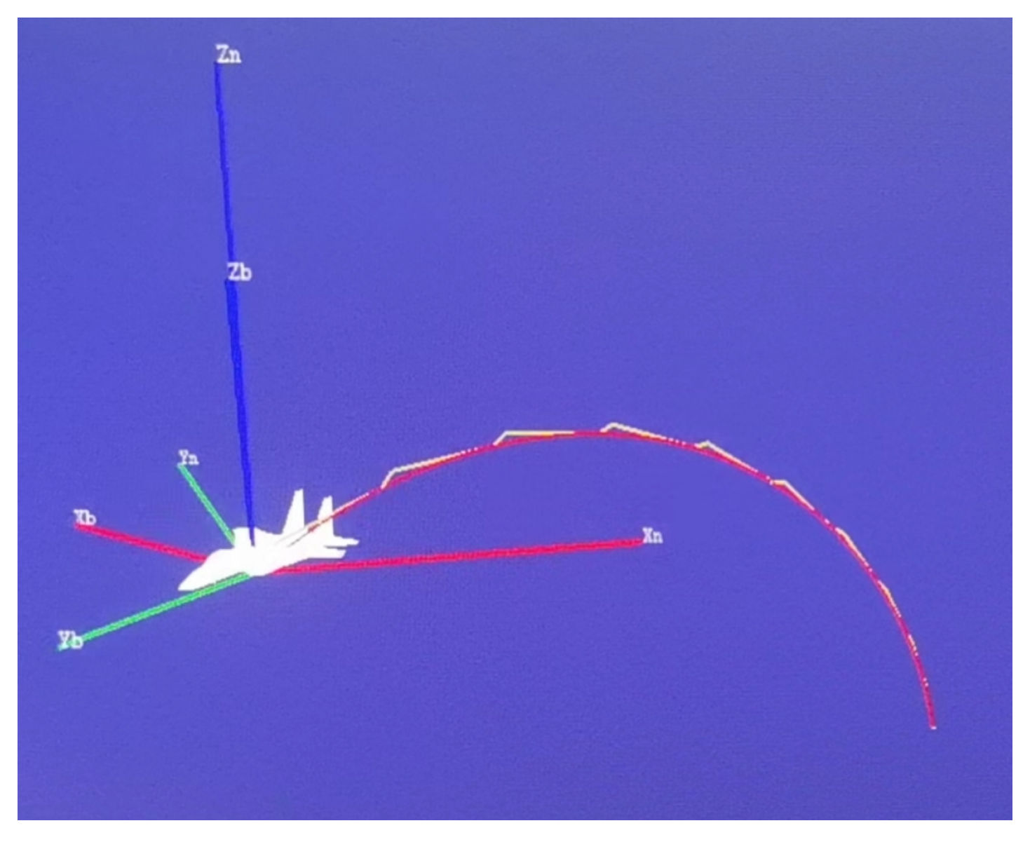
Figure 2.
Error comparison of 2nd-order extrapolation DR algorithm in the vertical plane to the real trajectory.
Figure 2.
Error comparison of 2nd-order extrapolation DR algorithm in the vertical plane to the real trajectory.
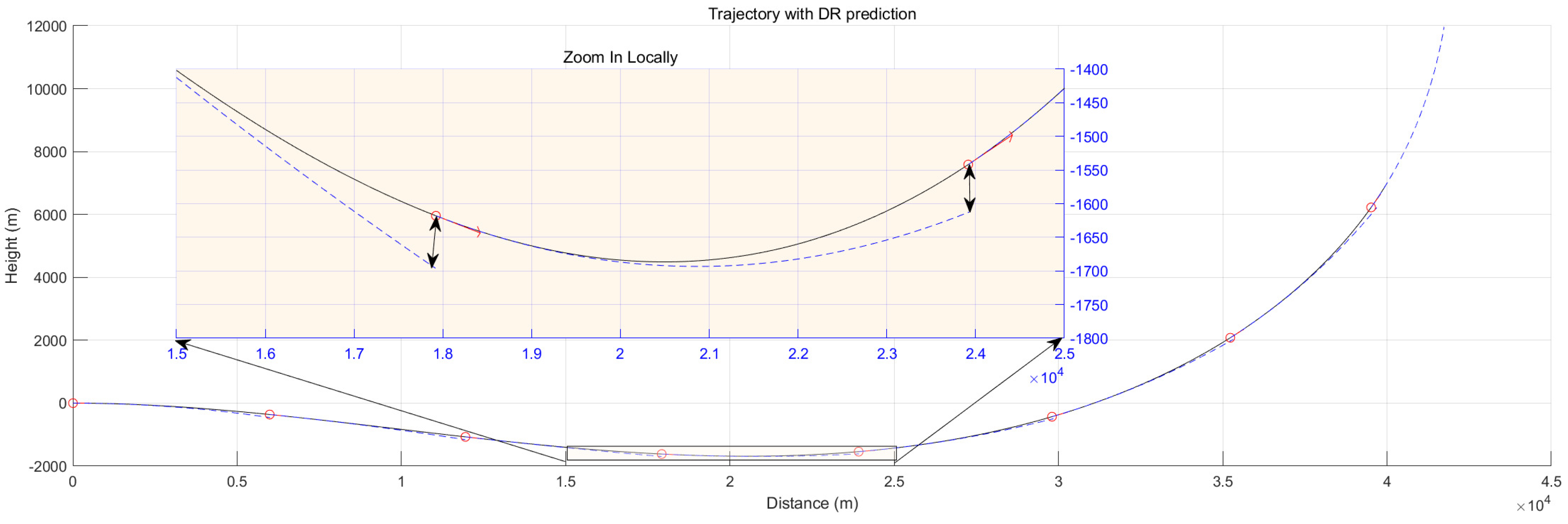
Figure 3.
Schematic diagram of navigation guidance parameters in a two-dimensional plane.
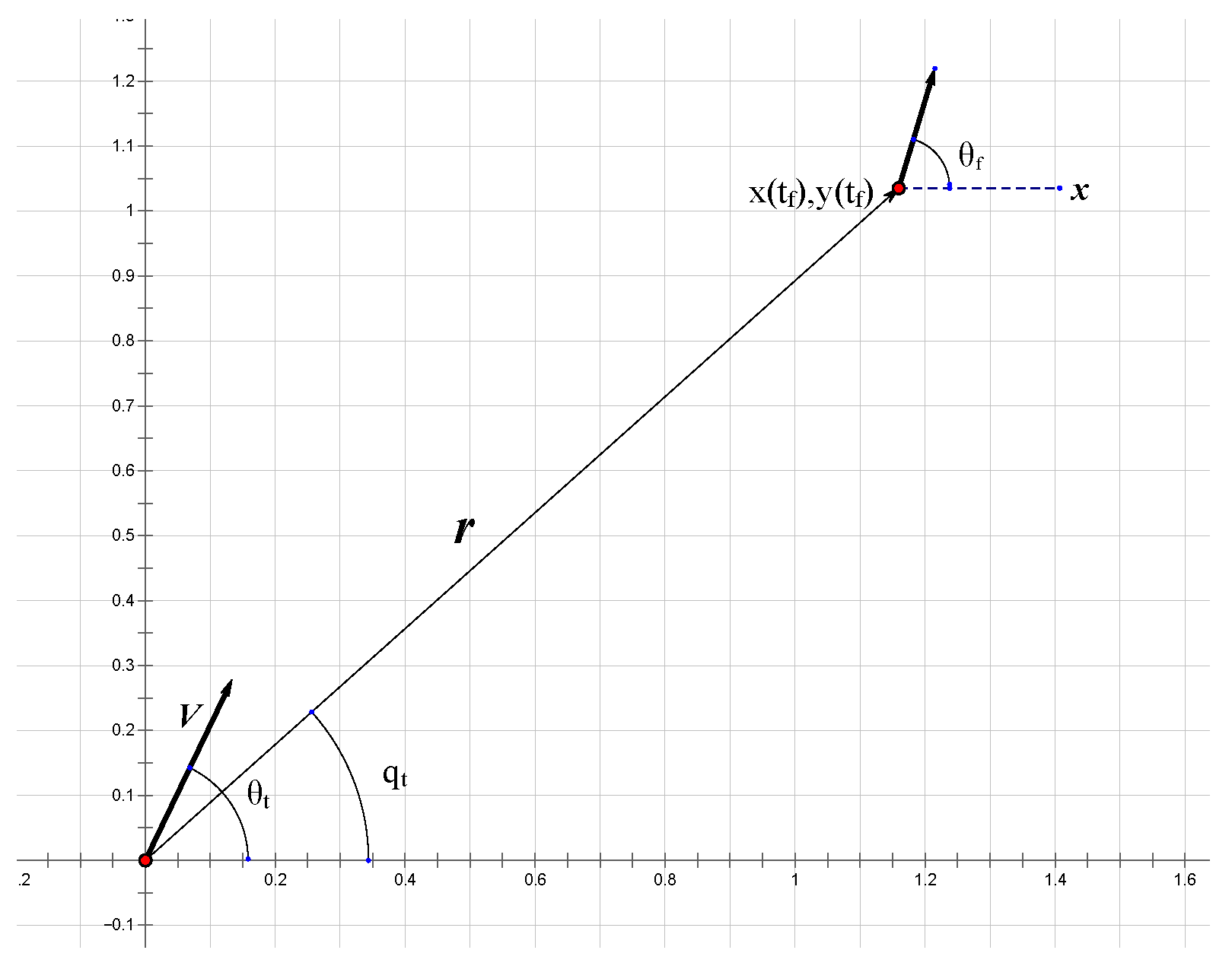
Figure 4.
The points on the 1st, 15001st and 30001st trajectory lines were taken as sampling points and the parameter circles were obtained
Figure 4.
The points on the 1st, 15001st and 30001st trajectory lines were taken as sampling points and the parameter circles were obtained
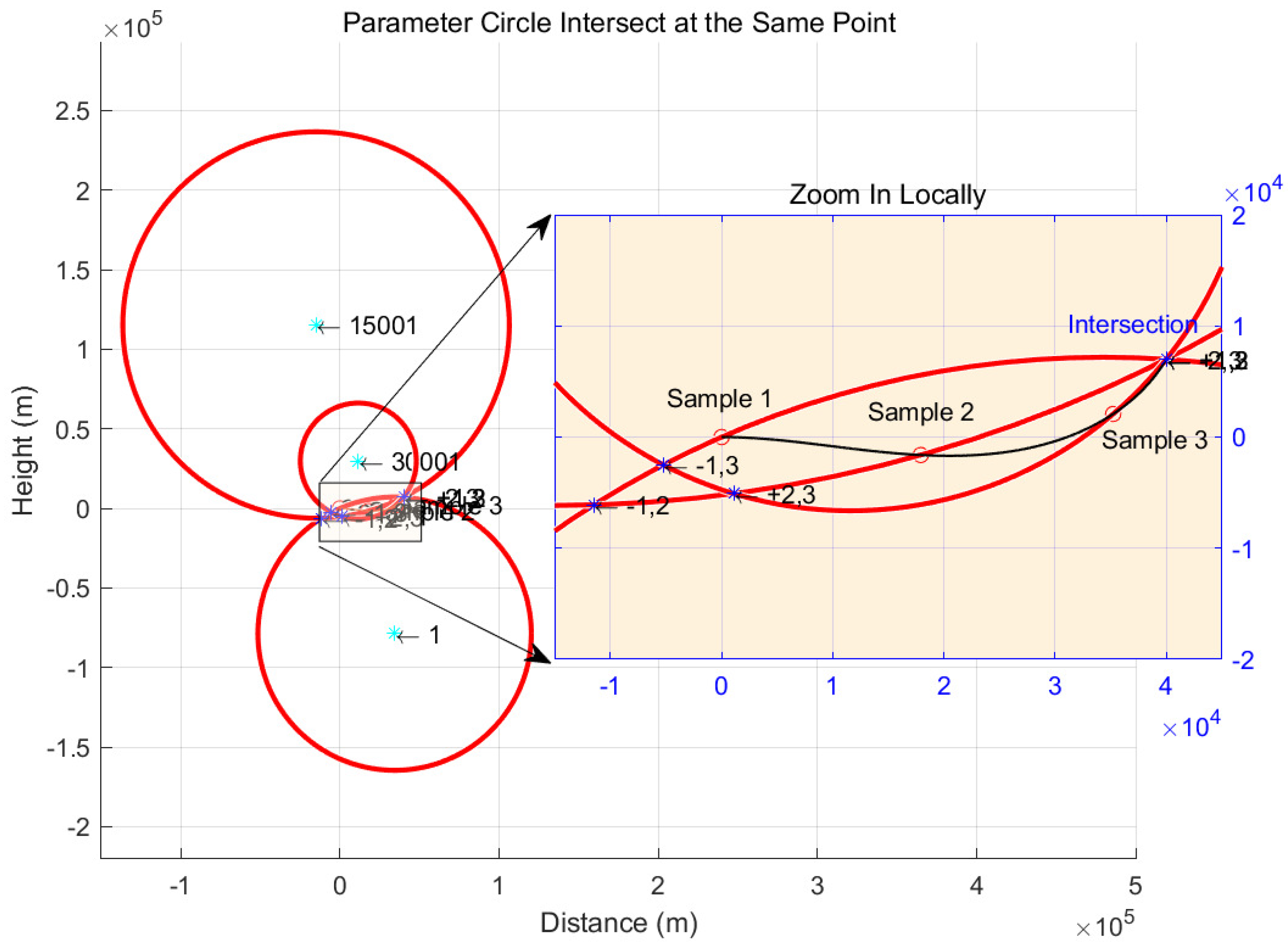
Figure 5.
The form of the intersection is affected by the parametric circle (there may be 2 intersections, 1 double root, or conjugate double root)
Figure 5.
The form of the intersection is affected by the parametric circle (there may be 2 intersections, 1 double root, or conjugate double root)
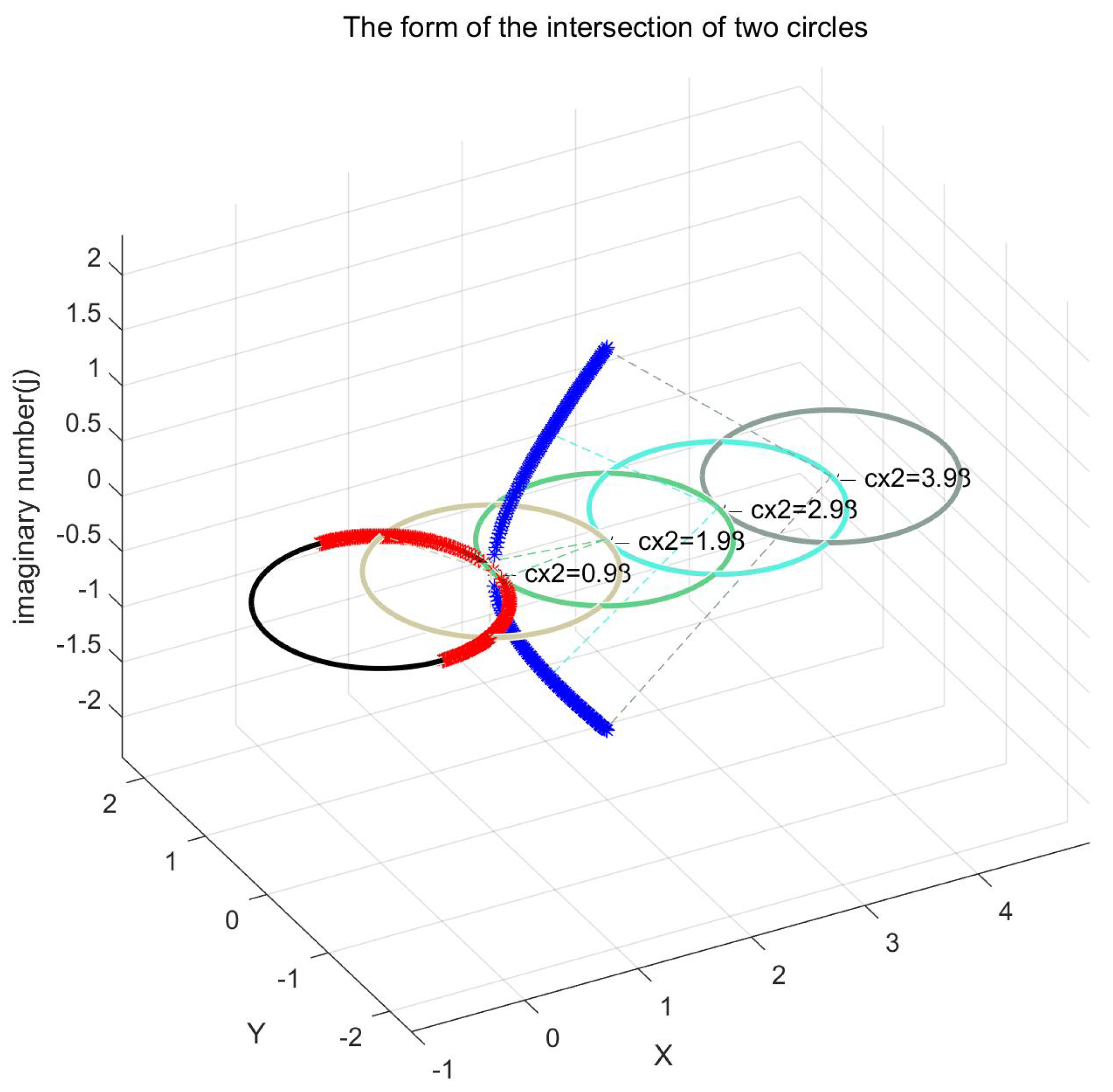
Figure 6.
In the numerical simulation, the blue curve is the trajectory line, the small red ring on the trajectory line is the sampling point, and the three large circles are the parameter circles that are solved and intersect at the desired end point of the trajectory.
Figure 6.
In the numerical simulation, the blue curve is the trajectory line, the small red ring on the trajectory line is the sampling point, and the three large circles are the parameter circles that are solved and intersect at the desired end point of the trajectory.
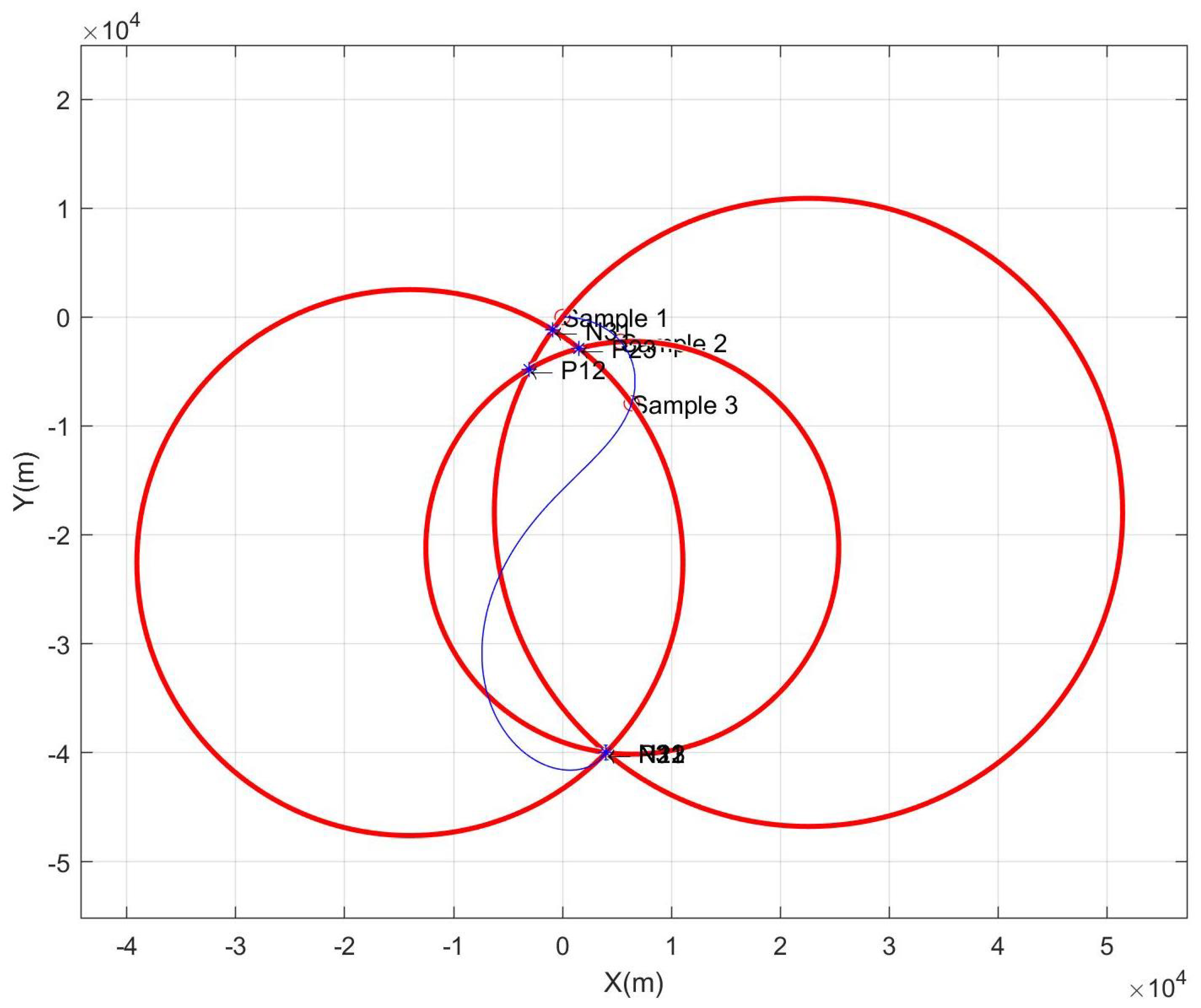
Figure 7.
The optimization iterative process of the 8 branches of 8B-PGDM. Only the 7 th branch has significantly converged to after 9 iterations.
Figure 7.
The optimization iterative process of the 8 branches of 8B-PGDM. Only the 7 th branch has significantly converged to after 9 iterations.
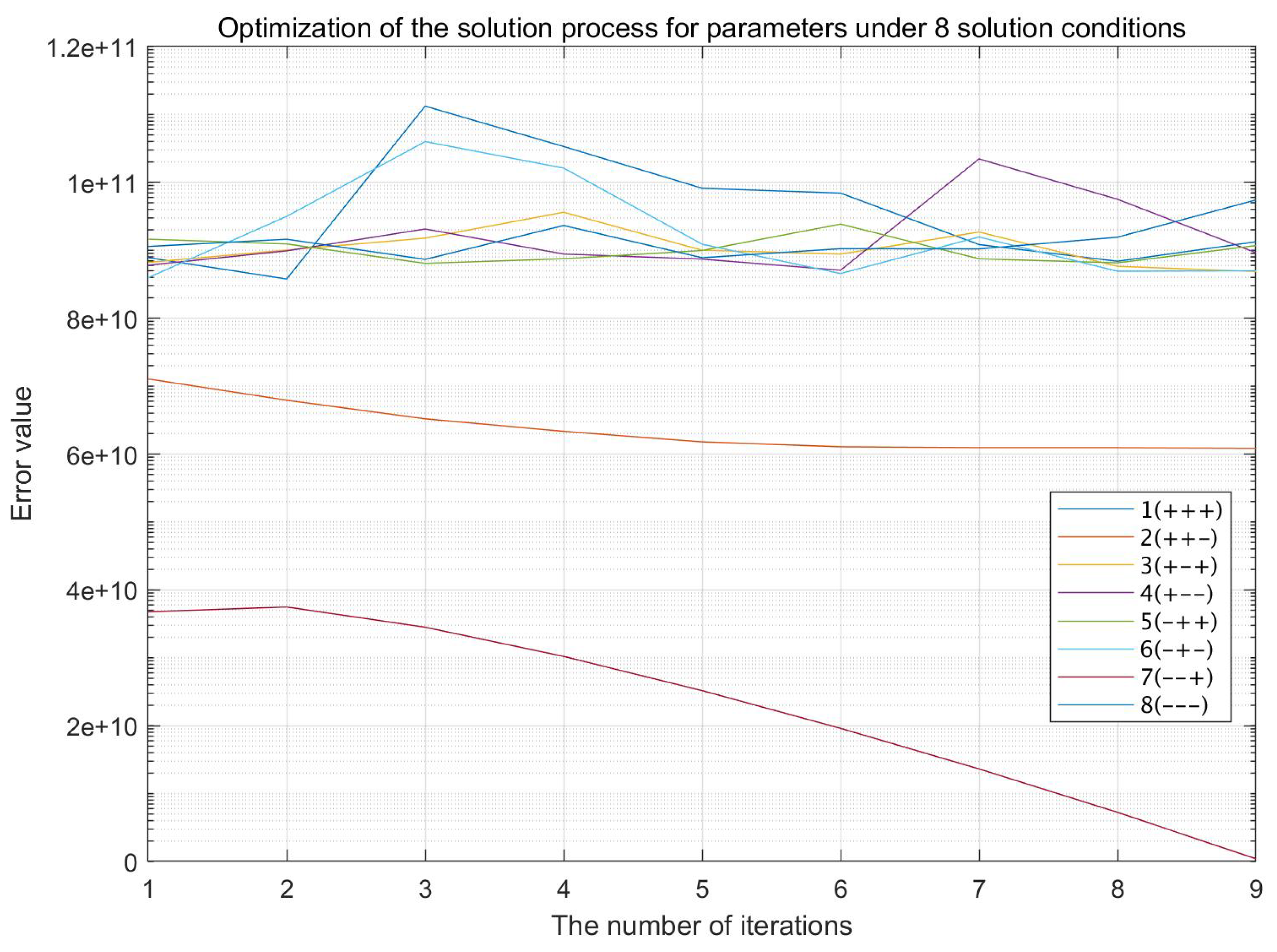
Figure 8.
Comparison of our method with traditional methods, our 8B-PGDM has advantage in sampling times, smooth curve estimation, and small cumulative error.
Figure 8.
Comparison of our method with traditional methods, our 8B-PGDM has advantage in sampling times, smooth curve estimation, and small cumulative error.
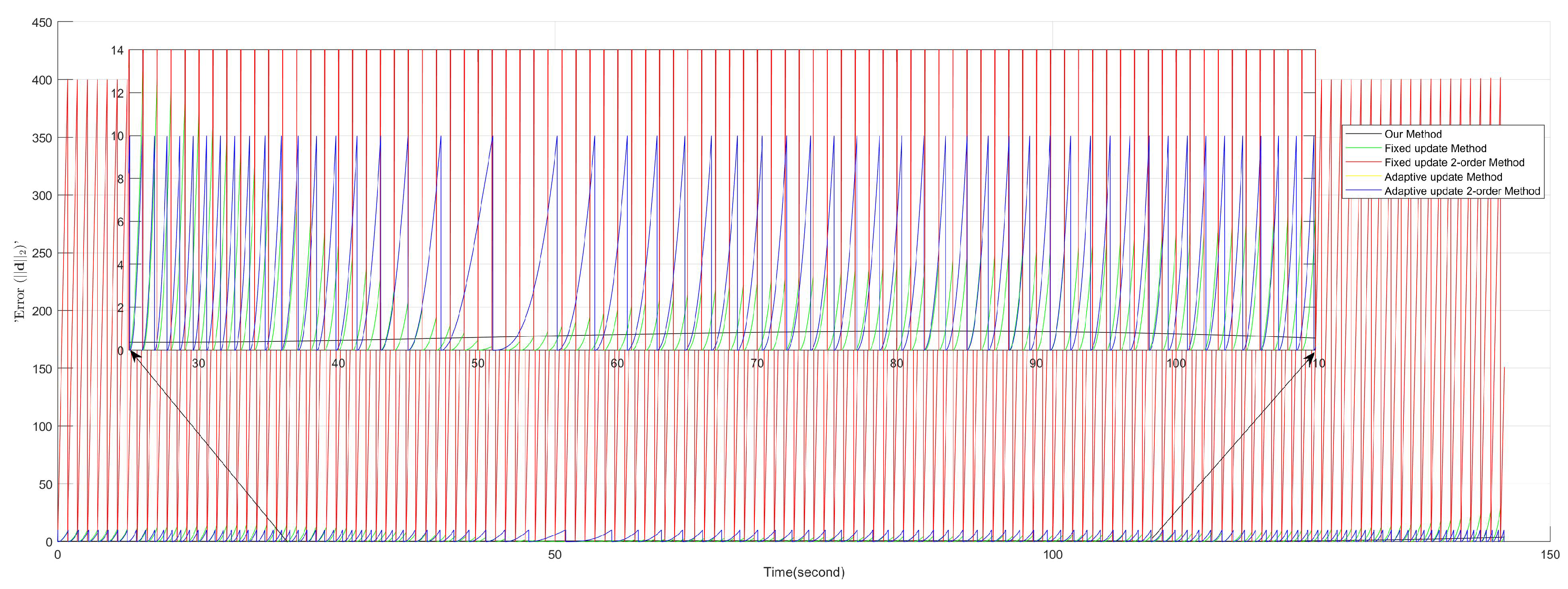

Table 1.
Experimental Results Comparison of Different Methods
| Method | Update Criteria | Samples | MSE |
| 8B-PGDM | - | 3 | 0.94459 |
| 1st-order DR | 1s | 146 | 18.053 |
| 2nd-order DR | 1s | 146 | 53176 |
| 1st-order DR | 122 | 19.913 | |
| 2nd-order DR | 122 | 19.913 |
Disclaimer/Publisher’s Note: The statements, opinions and data contained in all publications are solely those of the individual author(s) and contributor(s) and not of MDPI and/or the editor(s). MDPI and/or the editor(s) disclaim responsibility for any injury to people or property resulting from any ideas, methods, instructions or products referred to in the content. |
© 2025 by the authors. Licensee MDPI, Basel, Switzerland. This article is an open access article distributed under the terms and conditions of the Creative Commons Attribution (CC BY) license (http://creativecommons.org/licenses/by/4.0/).
Copyright: This open access article is published under a Creative Commons CC BY 4.0 license, which permit the free download, distribution, and reuse, provided that the author and preprint are cited in any reuse.


