
Submitted:
20 October 2025
Posted:
21 October 2025
You are already at the latest version
Abstract
This research presents a study on enhancing the localization and orientation accuracy of indoor Autonomous Guided Vehicles (AGVs) operating under a centralized, camera-based control system. We investigate and compare the performance of two Extended Kalman Filter (EKF) configurations: a standard EKF and a novel Blended EKF. The research methodology comprises four primary stages: (1) Sensor bias correction for the camera (CAM), Dead Reckoning, and Inertial Measurement Unit (IMU) to improve raw data quality; (2) Calculation of sensor weights using the Inverse-Variance Weighting principle, which assigns higher confidence to sensors with lower variance; (3) Multi-sensor data fusion to generate a stable state estimation that closely approximates the ground truth (GT); and (4) A comparative performance evaluation between the standard EKF, which processes sensor updates independently, and the Blended EKF, which fuses CAM and DR measurements prior to the filter’s update step. Experimental results demonstrate that the implementation of bias correction and inverse-variance weighting significantly reduces the Root Mean Square Error (RMSE) across all sensors. Furthermore, the Blended EKF not only achieved a lower RMSE in certain scenarios but also produced a notably smoother trajectory compared to the standard EKF. These findings indicate the significant potential of the proposed approach in developing more accurate and robust navigation systems for AGVs in complex indoor environments.
Keywords:
indoor AGV localization
; extended Kalman filter
; sensor fusion
; bias correction
; inversevariance weighting
1. Introduction
A centralized, vision-based control architecture for Autonomous Guided Vehicles (AGVs) offers a cost-effective alternative to systems reliant on expensive onboard sensors like LIDAR [9]. In industrial environments, positioning accuracy is critical [21]. This approach, often termed "infrastructure-based control," transfers complex navigation and fleet management tasks from individual vehicles to a powerful central server, enabling sophisticated coordination while reducing per-vehicle hardware costs [13]. The system’s core components include a network of CCTV cameras, a central processing server, a wireless communication network, and the vehicles themselves. The cameras provide a global "God’s-eye view" of the operational area, tracking vehicles and obstacles in real-time. This centralized vision approach leverages advances in computer vision and deep learning techniques for robust localization, as demonstrated by recent work combining imaging sensors with deep convolutional neural networks (DCNNs) for AGV pose estimation [9]. The central server processes this visual data through fleet management software that handles localization, path planning, and traffic management using AI [6] and computer vision techniques [2]. The server then transmits simple motion commands, such as "move forward 5 meters," to the AGVs via wireless communication networks. Recent infrastructure-based vision studies demonstrate that overhead or roadside cameras can detect and track mobile robots reliably in real time, underscoring the practicality of centralized, vision-first approaches [20,25]. Yet long-term localization remains challenging due to illumination changes, occlusions, and drift. A systematic review highlights the need for robust filtering, cross-sensor redundancy, and adaptive models to sustain performance over extended periods [17]. The vehicles execute these commands precisely by utilizing onboard sensor fusion techniques, integrating data from multiple sensors including encoders for distance measurement and Inertial Measurement Units (IMUs) for orientation tracking [24]. Recent advances in sensor fusion have shown that passive wheel odometry can outperform traditional drive-wheel odometry in many scenarios, while IMU/AHRS integration significantly improves accuracy during angular motion [2]. Advanced filtering techniques, including hybrid Kalman-particle filters and trainable Extended Kalman Filters with adaptive noise models, have demonstrated improved localization accuracy and robustness in indoor AGV environments [13,24]. Ultrasonic sensors act as a final safety measure, preventing collisions with unforeseen obstacles that may be in the camera’s blind spots. This hybrid model significantly reduces the cost per vehicle by replacing expensive onboard LIDAR systems with lower-cost sensor combinations and allows for sophisticated, system-wide traffic optimization through centralized path planning algorithms [22]. Modern optimization approaches, such as hybrid Grey Wolf Optimization combined with Kalman corrections, have shown improved path predictability and collision avoidance capabilities for dense warehouse AGV operations [16,22]. However, this centralized approach relies heavily on the central infrastructure, making it vulnerable to single-point failures and potentially less flexible in dynamic environments compared to fully autonomous, SLAM-based robots that maintain complete onboard sensing and processing capabilities. Although the Extended Kalman Filter (EKF) has been widely used for AGV positioning [19] , its performance may degrade when raw sensor data have different characteristics, such as camera (CAM) data with high noise and low update rate, compared to Dead Reckoning data with high update rate but prone to accumulated errors (drift). The normal EKF implementations often treat each sensor measurement update independently, which can lead to inconsistencies and non-smooth trajectory estimates, particularly when one sensor is prone to high noise or sudden disturbances. This highlights the research gap in developing an efficient data fusion strategy that can blend data from different sensors before feeding it to the filter update stage. Therefore, the contribution of this paper is to propose and evaluate a novel Blended EKF, which pre-fuses CAM and DR data using a weighted blending strategy before sending the data to the EKF. It is hypothesized that this approach not only reduces the positioning error but also produces smoother and more stable trajectories compared to the Normal EKF in an indoor environment.
2. Materials and Methods
This research presents an integrated approach for indoor localization of automated guided vehicles (AGVs) using multiple low-cost sensors, including cameras (CAMs), encoders, inertial measurement units (IMUs), and approximate positioning (Dead Reckoning - DR) [7].
2.1. Preparation and Equipment Used in the Experiment
2.1.1. Preparation Used in the Experiment
The BALTY AGV robot used in the experiment were equipped with specified sensors. Data from the encoder and IMU were recorded at a sampling rate of 10 Hz (every 0.1 s), while data from the camera (CAM) for absolute positioning were recorded at a rate of 5 Hz (every 0.2 s) [12]. To ensure the accuracy and consistency of the data used in the data fusion process, two data sampling scenarios were defined: (1) using the original sampling rate, with the IMU and Wheel Encoder set at 10 Hz and the CAM at 5 Hz, and (2) adjusting the sampling rate of all sensors to 5 Hz to create temporal consistency and facilitate efficient joint processing. Since the data from each sensor is collected asynchronously, a temporal alignment using an event-based synchronization method was performed in the post-processing step, with the “AGV starting point” set as the reference marker for synchronizing the entire dataset. For data communication between sensors, the MQTT protocol is used, which is set to a basic Quality of Service (QoS) level, prioritizing data transmission speed. However, this approach may result in some data loss in cases of unstable Wi-Fi network signals. The Ground Truth (GT) data is obtained by recording the AGV movement video using a top-view camera. Then, the image is processed frame by frame to extract the AGV position using Camera Calibration and Coordinate Transformation [3]. Reference positions on the experimental field are established as ground truth coordinates, which serve as a reference data set to assess the accuracy and errors of the sensors, as well as to perform error correction and evaluate the overall system performance [21].
2.1.2. Equipment Used in the Experiment
In this experiment, various sensors were installed to determine the grid position at (Table 1). An encoder coupled to a DC motor (JGB37-520) provides an AB-phase quadrature signal of 90 pulses per revolution, which is used to calculate the distance and direction of rotation. The WitMotion WT901C Inertial Measurement Unit (IMU) is a 9-DOF sensor that can measure linear acceleration (±16 g) and rotation rate (up to ±2000 °/s) and is set to output data at a frequency of 10 Hz. For image sensing, a TP-Link Tapo C200 camera was installed in a 4x8m the experimental area (Figure 1), which supports Full HD (1080p) recording at 30 frames per second. The data from these three sensors is used to integrate the data, which helps the system determine the position of the AGV.
2.1.3. IoT System Architecture Concepts
The conceptual framework for the IoT system architecture for AGV localization (Figure 2) is designed to collect, synchronize, and integrate data between multiple sensors and a central processing unit. This architecture consists of four main layers:
- Sensor (Sensor) Layer: Consists of the encoder + IMU and a CCTV camera that records data from the experimental area.
- Network (Communication) Layer: Uses Wi-Fi wireless communication with the MQTT protocol for lightweight messaging to exchange sensor data with low latency.
- Processing Layer (Central Server): The central server collects sensor data streams, performs synchronization, integrates the data, and stores the records for analysis.
- Application Layer: Provides visualization and location identification for the experimental area.
2.2. Localization Methods
Multi-sensor fusion works to determine the position and orientation of the AGV by combining data from internal sensors (e.g., encoder, IMU) with external sensors (e.g., camera) using EKF [11] with encoder, IMU, and camera.
2.2.1. Dead Reckoning Localization
Dead Reckoning estimation, which estimates the position of an AGV based on its previous state and movement data, is divided into two parts: measuring the distance from the wheels (encoder)and the direction from the IMU. This method is widely used in positioning research [5,18,23]. The state vector for Dead Reckoning is defined as
which represents the Cartesian coordinates and heading angle of the AGV. The AGV’s motion can be estimated using a kinematic motion model using the linear velocity v and angular velocity data from the sensors, as shown in the equation:
When integrating this equation with respect to time , the state update is obtained as follows:
where k is the current time index and is the previous time index. The data and are obtained by fusing data from:
- Distance measurement from encoder: An encoder mounted to the drive motor provides wheel rotation data that is converted to linear velocity and angular velocity using the vehicle kinematics model. However, This method is limited by accumulated errors caused by wheel slip, calibration inaccuracies, and surface irregularities [18,23].
- Direction from IMU: A 9-DOF IMU provides angular velocity and linear acceleration . The gyroscope output is crucial for direction calculations, as accelerometer data is highly sensitive to noise and bias errors that increase with time [8].
2.2.2. Camera Localization
To address the accumulated drift of Dead Reckoning (DR) that cannot be corrected with internal sensor data, external sensors, such as cameras, LiDAR, or CCTV, are used to measure the position based on world coordinates, thus correcting the position estimate. [5]. The process is as follows:
- Feature Detection: The system detects the features of the AGV to be located using standard computer vision algorithms.
- Coordinate Transformation: The AGV’s position in the image plane is converted to its real-world coordinates (world frame) via perspective transformation or a pre-calibrated homography matrix.
The measurement values obtained from this camera, , are crucial for making the system observable, meaning that important system states (such as position and velocity) can be estimated. [8]
The measurement values, , are fed into a filter for interpolation and prediction of through a nonlinear measurement model, h, noise, as shown in the equation:
These measurement values are then used in a Kalman Filter to calculate the innovation or error of the measurement, :
The accuracy of coordinate transformation and feature detection is crucial because they affect the accuracy of , which is a key factor in reducing the cumulative error of the DR.
2.3. Pre-Processing Data Analysis
Before data from different sensors can be fed through the data fusion process, it is essential to perform a pre-processing step to reduce bias and increase the reliability of the input data. This step consists of two main steps designed to apply bias correction and appropriately weight each sensor based on its statistical variance. An overview of all these pre-processing steps is shown in Figure 3 . The next subsections describe each step in detail.
2.3.1. Bias Correction
Before using the raw sensor data in the fusion process, the systematic bias of each sensor is assessed and corrected [15]. This is done by calculating the average deviation between the measured sensor value S and the reference value from the Ground Truth (GT) according to the equation:
Where is the measured value from the sensor at time t and is the reference value from the true path GT at the same time. The corrected value is then given by:
This process reduces the Root Mean Squared Error (RMSE) of the raw data and improves the reliability of the data. [10].
2.3.2. Inverse-Variance Weighting
Data from the error-corrected sensors are weighted statistically using the Inverse-Variance Weighting [4] method. This method assumes that sensors with low error variance are given higher weights during data fusion. The weight for each sensor i is calculated from the error variance as follows:
The weights are then normalized to Normalized Weights so that the sum of all weights is 1, defined as:
where M is the total number of sensors.
2.4. Extended Kalman Filter (EKF)
This research developed and compared the performance of two Extended Kalman Filter (EKF) models to estimate the state of an AGV, consisting of its position (X, Y axes) and heading. The state equations and measurement equations used in the EKF system can be written in the following general form: [13]:
Where: is the AGV state vector (position and direction), is the state transition function, is the control data from the IMU and encoder, is the process noise, is the measured value from the sensor, is the measurement function, is the measurement noise.
2.4.1. Normal Series Fusion EKF (Normal EKF)
A typical EKF operates using an iterative process consisting of two main steps: Prediction Step and Update Step[1] Prediction Step:
In this step, the EKF uses the AGV’s motion model, combined with data from the IMU and DR (encoder) sensors to predict the AGV’s next state (position and direction) based on the predicted state values. and the variance of the estimate (covariance) According to the equation:
where and is the predicted state and covariance, is the Jacobian matrix of the state transition function f, and is the process noise covariance of the system.
Update Step:
When new measurements from a sensor (e.g., a CAM) are received, the EKF uses them to update the predictions.
The Kalman Gain is calculated to determine the appropriate weight between the predicted and actual measured values. Then, the state and covariance are updated according to the equation:
where is the Jacobian matrix of the measurement function h, and is the measurement noise covariance.
A conventional EKF updates its values using measurements from each sensor separately. In sequential updating.
2.4.2. Blended EKF
The purpose of Blended EKF is to correct for the characteristics of Camera-Based Reckoning (CAM) and Dead Reckoning (DR) measurements. While CAM provides drift-free absolute position data, it suffers from high noise, inconsistent update rates, and occasional occlusions. DR, on the other hand, provides relative motion estimates, but inevitably accumulates drift over time. The raw data causes EKF to be unsmooth, as it alternates between noisy camera updates and drifting DR estimates. To correct for this, CAM and DR measurements are pre-blended prior to the update step. This blending produces a more stable and consistent measurement input, which reduces oscillations and produces a smoother trajectory.
The Blended EKF method fuses measurements from the Camera (CAM) and Dead Reckoning (DR) before the update process. User-defined weights are used to control the proportion of influence of each measurement source. This can be written as the following equation:
where:
- is the weight assigned to the Camera (CAM) measurements
- is the weight assigned to the Dead Reckoning (DR) measurements
To achieve balance in the aggregation, the following conditions are defined. Normalization:
The uncertainty of the mixed measurement covariance, or , can be estimated as:
The selection of the values of and may be based on experimental testing or tuning to suit the actual application environment.
3. Experimental Design
This experiment aimed to evaluate the performance of AGV location identification using fusion of data from multiple sensors.The main equipment used in this experiment is the AGV BALTY and various sensors, shown in Figure 4. The experimental design was structured and controlled to generate reliable data for analysis. The experimental data processing steps consisted of the following:
-
Bias Correction Analysis: The raw data obtained from each sensor type were analyzed against Ground Truth (GT) data, which is akin to the "true path," to determine the systematic bias and variance.This step is crucial in reducing the Root Mean Squared Error (RMSE) of the raw data and enhancing the reliability of the data before further use.
- Weighting with Inverse-Variance Weighting: The error-corrected data were then statistically weighted. The principle is that sensors with lower bias variance (which means higher reliability) will receive higher weight in data fusion.
- Data Fusion with EKF: The pre-processed data is fed into the EKF system to estimate the state (position and orientation). Two EKF models have been developed and compared: (1) a conventional EKF and (2) a blended EKF, which fuses measurements from the CAM and DR sensors before the update process.
To ensure that the performance evaluation covers real-world application scenarios, the AGV was tested to move along a specially designed route, which consists of two main parts:
- Straight Section: This movement involves constant speed and no sudden changes of direction to assess the ability to maintain a precise position under normal conditions.
- Curved Section: It is a dynamic movement, which easily causes accumulated drift in the dead reckoning system to assess the system capability and stability under the condition of changing direction of movement.
The experiment starts at x=0, y=7, moves in a straight line, stops at position x=1, y=7, then rotates and moves in a straight line again, then stops the movement, which is a comprehensive experiment to test the accuracy and stability under the conditions of movement.
4. Results and Discussion
This section presents and discusses experimental results obtained from sensor data analysis and data fusion, focusing on evaluating the performance of the designed algorithmic location system.
4.1. Analysis of bias correction (BC) results
Bias correction improves the accuracy of the sensor, particularly its positioning. The analysis of the average bias errors of each sensor used in the experiment reveals the limitations and basic accuracy of the sensor before its application. Table 2 shows the average sensor error values at two sampling rates (dt), 0.1 s and 0.2 s, the sensor’s data acquisition frequency.
- Camera Sensor (CAM): The bias error values in the X-axis (Mean Error X) and Y-axis (Mean Error Y) were found to be positive in both cases ( = 0.1 and 0.2). The position was higher than the actual values in both axes. However, the camera sensor did not measure the rotation angle, so there was no error for the Mean Error .
- Dead Reckoning (DR) Sensor: For DR, the error values in the X-axis (Mean Error X) were negative, while the Y-axis (Mean Error Y) were positive, indicating that there was error in both directions.
- Inertial Measurement Unit (IMU) Sensors: IMU sensors are used to measure changes in angle (). The only error is the Mean Error ().
Different types of sensors have different bias tolerances, both in direction (positive/negative) and magnitude. This information is used to develop bias correction algorithms, and the analysis, using Root Mean Square Error (RMSE) values, was calculated for two sampling intervals: dt = 0.1 s and dt = 0.2 s (Table 3).
-
Camera Sensor (CAM):
- −
- Before Correction (Raw): CAM had RMSE X values of 0.0617 m and 0.0483 m, and RMSE Y values of 0.0467 m and 0.0459 m for s and s, respectively.
- −
- After Correction (Corrected): RMSE values significantly decreased, with RMSE X decreasing to 0.0536 m and 0.0414 m, and RMSE Y decreasing to 0.0382 m and 0.0355 m, respectively.
-
Dead Reckoning (DR) Sensor:
- −
- Before Correction (Raw): DR had RMSE X values of 0.0792 m and 0.0780 m, and RMSE Y values of 0.0241 m and 0.0255 m.
- −
- After Correction (Corrected): Error correction significantly reduced the RMSE of DR. RMSE X decreased to 0.0497 m and 0.0495 m, while RMSE Y decreased to 0.0148 m and 0.0157 m, respectively.
-
Inertial Measurement Unit (IMU) Sensor:
- −
- Before Correction (Raw): The IMU is used to measure the rotation angle (). The RMSE values before correction were approximately 0.2256 rad and 0.2317 rad.
- −
- After Correction (Corrected): The RMSE values decreased to approximately 0.2018 rad and 0.2072 rad.
The trajectories of the CAM and DR sensors before and after the aberration correction, compared to the ground truth (GT) trajectories at dt=0.1s and dt=0.2s, are shown Figure 5 and Figure 6 respectively.
- True Trajectory (GT): The blue line represents the actual trajectory of the object, which is the reference line.
- CAM (Raw): The dark blue dots represent the CAM path before correction.
- CAM (Bias-Corrected): The orange dots represent the CAM path after correction.
- DR (Raw): The green dots represent the DR path before correction.
- DR (Bias-Corrected): The red dots represent the DR path after correction.
Bias correction reduces sensor errors. The apparent decrease in RMSE values corresponds to a closer match of the corrected trajectory to the ground truth, demonstrating the importance of performing bias correction before data acquisition.
4.2. Analysis of the results of sensor data fusion using Inverse-Variance Weighting
Data from multiple sensors is combined using Inverse-Variance Weighting, a method that prioritizes low variance (i.e. high accuracy) data. Data from cameras (CAM), dead reckoning (DR), and inertial measurement units (IMU) are compared between raw data and bias corrected at dt=0.1s and dt=0.2s.
From Table 4 and Table 5, the variance values were used to determine the sensor weights via inverse-variance weighting, which assigns larger weights to measurements with lower variance. In particular, the dead reckoning (DR) sensor, having a very low Y-axis variance (), receives a high Y-axis weight (). Conversely, the camera (CAM) has a higher Y-axis variance, resulting in a lower weight (), while along the X-axis the similar variances lead to more balanced weights. For the rotation angle (), the inertial measurement unit (IMU)—as the sole information source—receives a weight of 1. These findings are consistent with the trajectory comparison in Figure 7 and Figure 8, where the bias-corrected trajectories lie closer to the ground truth.
Table 6, which shows the root mean square error (RMSE) values of the sensor data fusion, shows that bias-corrected data were obtained before fusion. Comparing the raw data and the fused data after bias correction, the RMSE of the bias-corrected data decreased on both the X and Y axes.
4.3. Analysis of data integration results using EKF
Indoor localization of an Automated Guided Vehicle (AGV) involves the fusion of data from multiple sensor sources to improve accuracy. The Extended Kalman Filter (EKF) is a popular choice due to its capability of handling nonlinearities. Therefore, two EKF models were compared: the EKF Normal (original, both raw and bias-corrected) and the EKF Blended (weighted with sensor values based on the parameters and ).
From Table 7, it can be seen that using the EKF with bias correction effectively reduces the RMSE error. The RMSE for is significantly reduced when using the corrected data compared to the raw data, both at and . Furthermore, applying the blended EKF provides even better results, minimizing the RMSE for when appropriate weighting coefficients (, ) are selected.
From Figure 9 and Figure 10, which compare the trajectories of the EKF filter, it is found that the trajectory obtained from the raw data (Normal RAW) deviates the most from the ground truth (GT), especially at dt=0.1s. However, when the data is normal bias corrected, the trajectory becomes closer to the GT, and the Blended EKF performs better, giving a smoother trajectory that is closest to the GT. Comparing the sampling periods (dt), it is found that at dt=0.1s, although it provides more detailed trajectory details, it also has more pronounced noise, while at dt=0.2s, it is smoother.
It is noteworthy that some weighting configurations of Blended EKF give lower RMSE values. Fusing higher and lower values leads to better performance. This result can be explained by Table 4 and Table 5, which shows that Dead Reckoning (DR) sensors have lower variance along the Y-axis compared to cameras (CAM), thereby increasing the reliability of DR measurements in that direction. Therefore, it is more prudent to assign more weight to DR along the Y-axis, which relies more on stable sensors, while CAM still performs better along the X-axis, which is comparable to DR. The importance of adjusting the blending coefficients to match the statistical values of each sensor to increase the accuracy and stability of the positioning.
4.4. Discussion and suggestions
The experiments demonstrate the advantages of Blended EKF, but there are some limitations. First, the experiment was conducted indoors in a controlled environment with fixed camera positions, which may not capture complex real-world conditions or have uncaptured points. Second, this analysis assumes that the deviations of each sensor are constant. In practice, sensor characteristics may change due to temperature, wear, or other disturbances, which may affect the bias correction process. Third, the blending coefficients (, ) were selected based on experimental performance.
This limitation provides a useful guideline for future research. Future studies could expand the experiments to larger or more complex environments and incorporate dynamic simulations, such as moving obstacles or the interaction of multiple automated guided vehicles (AGVs). Developing methods and compensating for time-varying biases is also important. Furthermore, adopting adaptive or machine-learning mechanisms to automatically adjust blending weights may contribute to the practical application of the proposed Blended EKF in industrial and logistics contexts.
5. Conclusions
This research has demonstrated an effective data fusion framework for the localization of Automated Guided Vehicles (AGVs) in indoor environments. The core of this framework, which incorporates bias correction and inverse-variance weighting, yielded a significant reduction in the Root Mean Square Error (RMSE) across all sensors, causing the corrected trajectories to align more closely with the ground truth (GT). This weighting method strategically assigns greater influence to more reliable sensor data, such as the high weight given to the Dead Reckoning (DR) sensor’s stable Y-axis measurements. The proposed Blended EKF methodology proved superior to the standard EKF. Not only did it achieve a lower RMSE in key scenarios, but it also produced a markedly smoother trajectory that demonstrated the highest fidelity to the ground truth. Furthermore, this study confirmed that fine-tuning the blending coefficients to reflect the statistical properties of each sensor enhances both accuracy and stability. Specifically, assigning greater weight to the DR sensor for the Y-axis and the Camera (CAM) for the X-axis minimized the overall RMSE.
In conclusion, the experimental results indicate that the proposed approach provides a low-cost, accurate, and robust localization solution, making it highly suitable for practical AGV applications in indoor settings.
Author Contributions
Conceptualization: N. K. and J. S., Methodology: N. K., S. K. and J. S., Software: N. K. and S. P., Validation: N. K. and J. S., Formal analysis: N. K. and S. S., Investigation: N. K. and J. S., Resources: N. K., S. K. and S. P., Data curation: N. K. and S. S., Writing-original draft presentation: N. K. and j. S., Writing-review and editing: J. S., N. K. and S. P., Visualization: N. K., Supervision: S. P., S. K. and J. S., Project administration: J. S., All authors have read and agreed to the published version of the manuscript.
Funding
This work was supported by Suranaree University of Technology.
Data Availability Statement
The datasets generated during and/or analyzed during the current study are available from the corresponding author upon reasonable request.
Acknowledgments
This work was supported by Suranaree University of Technology and Department of Mechatronics and Robotics Engineering, School of Engineering and Innovation, Rajamangala University of Technology Tawan-ok.
Conflicts of Interest
The authors declare no potential conflict of interests.
References
- Akhlaghi, S.; Zhou, N.; Huang, Z. Adaptive Adjustment of Noise Covariance in Kalman Filter for Dynamic State Estimation. 2017 IEEE Power & Energy Society General Meeting 2017, 1–5. [Google Scholar] [CrossRef]
- Bereszyński, K.; Pelic, M.; Paszkowiak, W.; Pabiszczak, S.; Myszkowski, A.; Walas, K.; Czechmanowski, G.; Węgrzynowski, J.; Bartkowiak, T. Passive Wheels – A New Localization System for Automated Guided Vehicles. Heliyon 2024, 10(15), e34967. [Google Scholar] [CrossRef] [PubMed]
- Brooks, A.; Makarenko, A.; Upcroft, B. Gaussian Process Models for Sensor-Centric Robot Localisation. In Proceedings of the 2006 IEEE International Conference on Robotics and Automation (ICRA 2006, 56–61. [CrossRef]
- Chen, Y.; Cui, Q.; Wang, S. Fusion Ranging Method of Monocular Camera and Millimeter-Wave Radar Based on Improved Extended Kalman Filtering. Sensors (Basel) 2025, 25. [Google Scholar] [CrossRef]
- Fan, Z.; Zhang, L.; Wang, X.; Shen, Y.; Deng, F. LiDAR, IMU, and Camera Fusion for Simultaneous Localization and Mapping: A Systematic Review. Artificial Intelligence Review 2025, 58(6), 174. [Google Scholar] [CrossRef]
- Fragapane, G.; de Koster, R.; Sgarbossa, F.; Strandhagen, J. O. Planning and Control of Autonomous Mobile Robots for Intralogistics: Literature Review and Research Agenda. European Journal of Operational Research 2021, 294(2), 405–426. [Google Scholar] [CrossRef]
- Grzechca, D.; Ziebinski, A.; Paszek, K.; Hanzel, K.; Giel, A.; Czerny, M.; Becker, A. How Accurate Can UWB and Dead Reckoning Positioning Systems Be? Comparison to SLAM Using the RPLidar System. Sensors (Basel) 2020, 20. [Google Scholar] [CrossRef]
- Hesch, J. A.; Kottas, D. G.; Bowman, S. L.; Roumeliotis, S. I. Camera–IMU-Based Localization: Observability Analysis and Consistency Improvement. The International Journal of Robotics Research 2013, 33(1), 182–201. [Google Scholar] [CrossRef]
- Ito, S.; Hiratsuka, S.; Ohta, M.; Matsubara, H.; Ogawa, M. Small Imaging Depth LIDAR and DCNN-Based Localization for Automated Guided Vehicle. Sensors (Basel) 2018, 18. [Google Scholar] [CrossRef]
- Khaleghi, B.; Khamis, A.; Karray, F. O.; Razavi, S. N. Multisensor Data Fusion: A Review of the State-of-the-Art. Information Fusion 2013, 14(1), 28–44. [Google Scholar] [CrossRef]
- Li, M.; Mourikis, A. I. High-Precision, Consistent EKF-Based Visual–Inertial Odometry. The International Journal of Robotics Research 2013, 32(6), 690–711. [Google Scholar] [CrossRef]
- Liu, Y.; Wang, S.; Xie, Y.; Xiong, T.; Wu, M. A Review of Sensing Technologies for Indoor Autonomous Mobile Robots. Sensors (Basel) 2024, 24. [Google Scholar] [CrossRef]
- Milam, G.; Xie, B.; Liu, R.; Zhu, X.; Park, J.; Kim, G.; Park, C. H. Trainable Quaternion Extended Kalman Filter with Multi-Head Attention for Dead Reckoning in Autonomous Ground Vehicles. Sensors (Basel) 2022, 22. [Google Scholar] [CrossRef]
- Niu, X.; Wu, Y.; Kuang, J. Wheel-INS: A Wheel-Mounted MEMS IMU-Based Dead Reckoning System. IEEE Transactions on Vehicular Technology 2021, 70(10), 9814–9825. [Google Scholar] [CrossRef]
- Perera, L. D. L.; Wijesoma, W. S.; Adams, M. D. The Estimation Theoretic Sensor Bias Correction Problem in Map Aided Localization. The International Journal of Robotics Research 2006, 25(7), 645–667. [Google Scholar] [CrossRef]
- Sousa, L. C.; Silva, Y. M. R.; Schettino, V. B.; Santos, T. M. B.; Zachi, A. R. L.; Gouvea, J. A.; Pinto, M. F. Obstacle Avoidance Technique for Mobile Robots at Autonomous Human–Robot Collaborative Warehouse Environments. Sensors (Basel) 2025, 25. [Google Scholar] [CrossRef] [PubMed]
- Sousa, R. B.; Sobreira, H. M.; Moreira, A. P. A Systematic Literature Review on Long-Term Localization and Mapping for Mobile Robots. Journal of Field Robotics 2023, 40(5), 1245–1322. [Google Scholar] [CrossRef]
- Teng, X.; Shen, Z.; Huang, L.; Li, H.; Li, W. Multi-Sensor Fusion Based Wheeled Robot Research on Indoor Positioning Method. Results in Engineering 2024, 22, 102268. [Google Scholar] [CrossRef]
- Urrea, C.; Agramonte, R. Kalman Filter: Historical Overview and Review of Its Use in Robotics 60 Years after Its Creation. Journal of Sensors 2021, 2021(1), 9674015. [Google Scholar] [CrossRef]
- Vignarca, D.; Vignati, M.; Arrigoni, S.; Sabbioni, E. Infrastructure-Based Vehicle Localization through Camera Calibration for I2V Communication Warning. Sensors (Basel) 2023, 23. [Google Scholar] [CrossRef]
- Wang, Q.; Wu, J.; Liao, Y.; Huang, B.; Li, H.; Zhou, J. Research on Multi-Sensor Fusion Localization for Forklift AGV Based on Adaptive Weight Extended Kalman Filter. Sensors (Basel) 2025, 25. [Google Scholar] [CrossRef]
- Xu, H.; Li, Y.; Lu, Y. Research on Indoor AGV Fusion Localization Based on Adaptive Weight EKF Using Multi-Sensor. Journal of Physics: Conference Series 2023, 2428, 012028. [Google Scholar] [CrossRef]
- Yan, Y.; Zhang, B.; Zhou, J.; Zhang, Y.; Liu, X. Real-Time Localization and Mapping Utilizing Multi-Sensor Fusion and Visual–IMU–Wheel Odometry for Agricultural Robots. Agronomy 2022, 12. [Google Scholar] [CrossRef]
- Zeghmi, L.; Amamou, A.; Kelouwani, S.; Boisclair, J.; Agbossou, K. A Kalman–Particle Hybrid Filter for Improved Localization of AGV in Indoor Environment. In Proceedings of the 2nd International Conference on Robotics, Automation and Artificial Intelligence (RAAI), 141–147. 2022. [Google Scholar] [CrossRef]
- Zheng, Z.; Lu, Y. Research on AGV Trackless Guidance Technology Based on the Global Vision. Science Progress 2022, 105(3), 00368504221103766. [Google Scholar] [CrossRef]
Figure 1.
Illustration of the experimental area showing the four CCTV camera placements around the m testbed. Each camera covers a specific quadrant to provide full-area visual tracking of the AGV.
Figure 1.
Illustration of the experimental area showing the four CCTV camera placements around the m testbed. Each camera covers a specific quadrant to provide full-area visual tracking of the AGV.
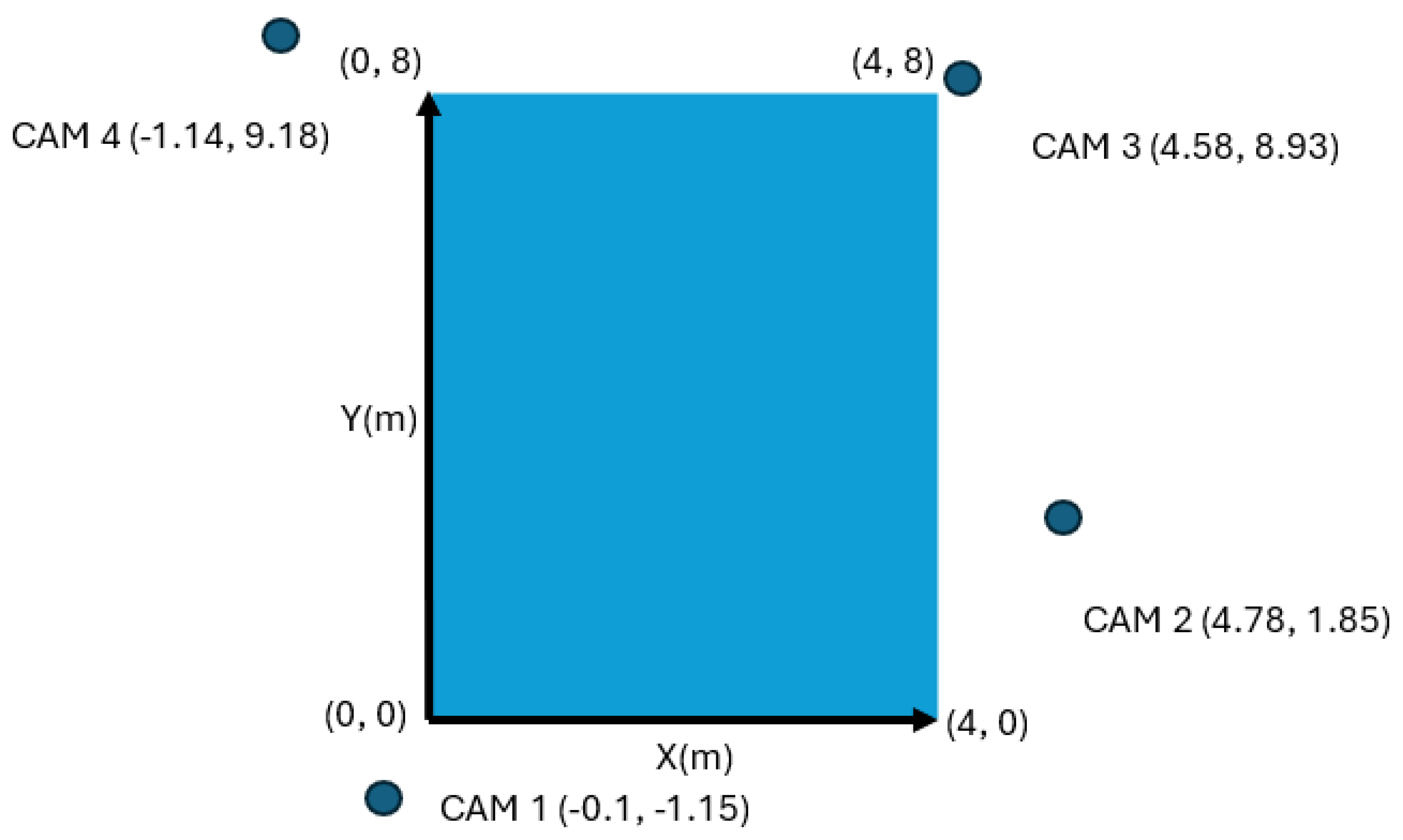
Figure 2.
IoT system architecture for AGV localization. The framework consists of three layers: the perception layer (sensors such as UWB, IMU, and encoders), the network layer (wireless data transmission via Wi-Fi or MQTT), and the application layer (central server performing sensor fusion and control via the EKF).
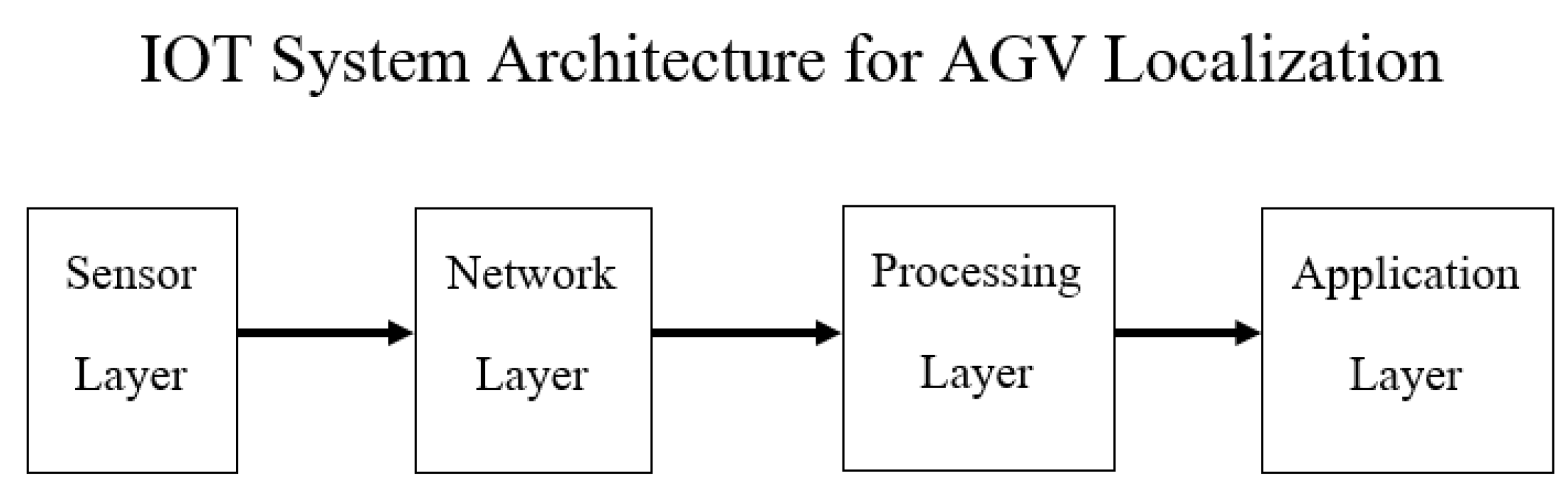
Figure 3.
Data pre-processing workflow for multi-sensor fusion. The process includes noise filtering, time synchronization, bias correction, and resampling to align data from Camera, IMU, and encoder sensors prior to fusion using the Extended Kalman Filter (EKF).
Figure 3.
Data pre-processing workflow for multi-sensor fusion. The process includes noise filtering, time synchronization, bias correction, and resampling to align data from Camera, IMU, and encoder sensors prior to fusion using the Extended Kalman Filter (EKF).
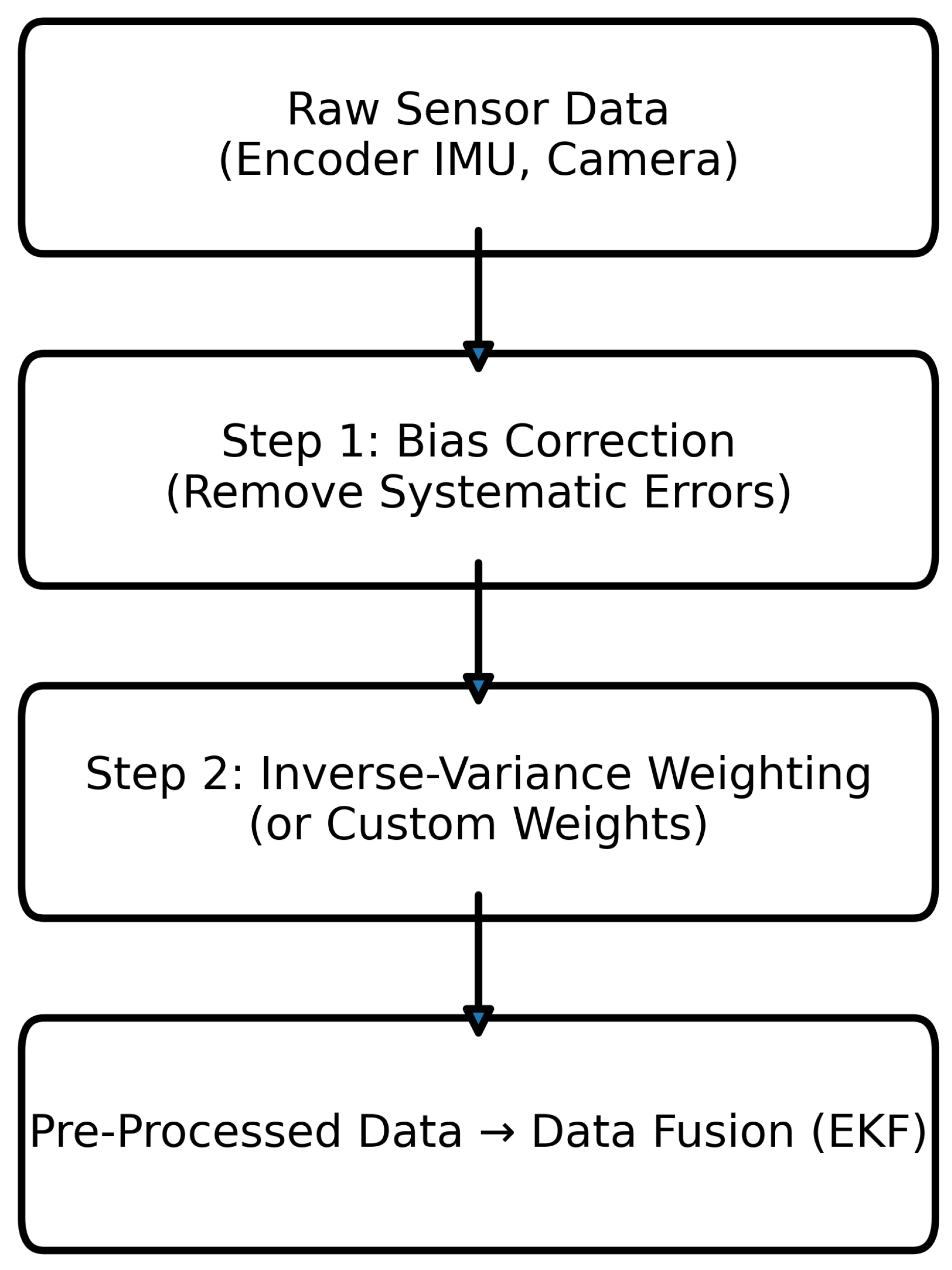
Figure 4.
Experimental equipment used for AGV localization: (a) AGV BALTY; (b) CCTV; (c) reference camera; (d) motor encoder; and (e) IMU.
Figure 4.
Experimental equipment used for AGV localization: (a) AGV BALTY; (b) CCTV; (c) reference camera; (d) motor encoder; and (e) IMU.
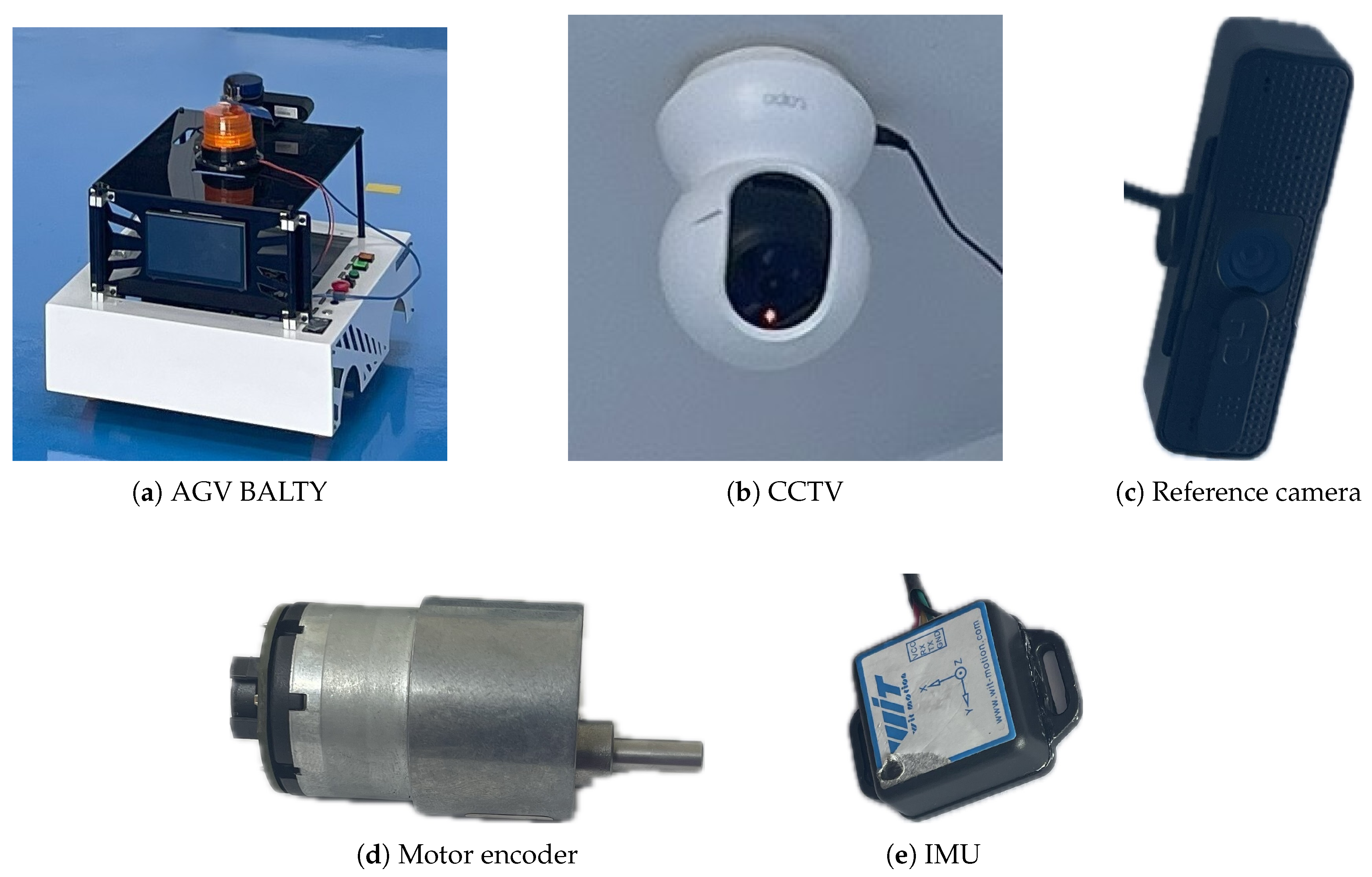
Figure 5.
Trajectory comparison of ground truth (GT) and sensor data (CAM and DR): Raw vs Bias-Corrected (BC) at s.
Figure 5.
Trajectory comparison of ground truth (GT) and sensor data (CAM and DR): Raw vs Bias-Corrected (BC) at s.
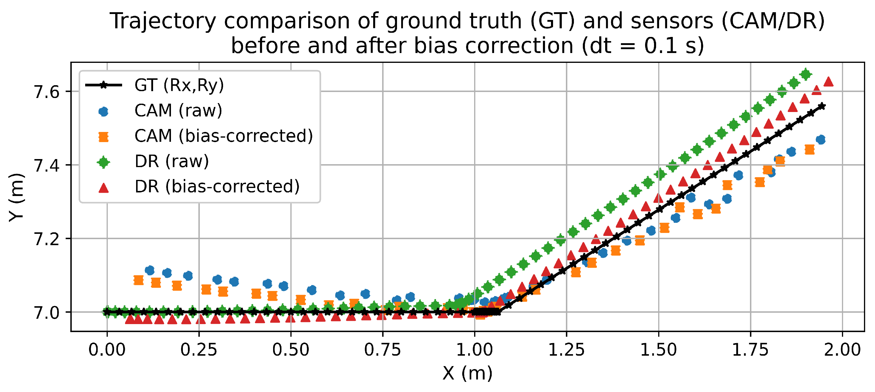
Figure 6.
Trajectory comparison of ground truth (GT) and sensor data (CAM and DR): Raw vs Bias-Corrected (BC) at s.
Figure 6.
Trajectory comparison of ground truth (GT) and sensor data (CAM and DR): Raw vs Bias-Corrected (BC) at s.
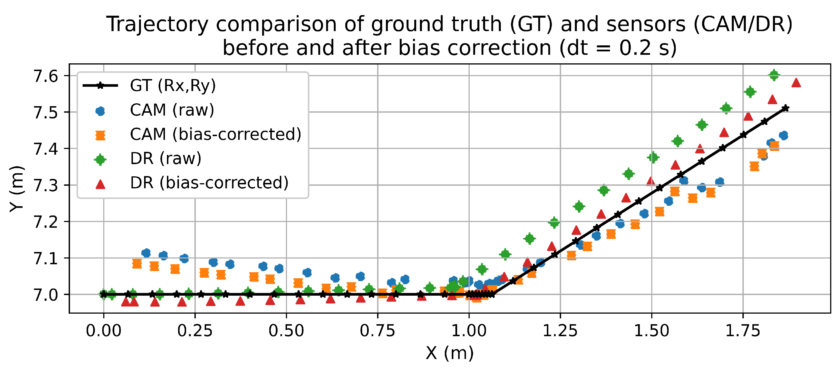
Figure 7.
Trajectory comparison between the ground truth (GT) and fused data (raw and bias-corrected) at s.
Figure 7.
Trajectory comparison between the ground truth (GT) and fused data (raw and bias-corrected) at s.
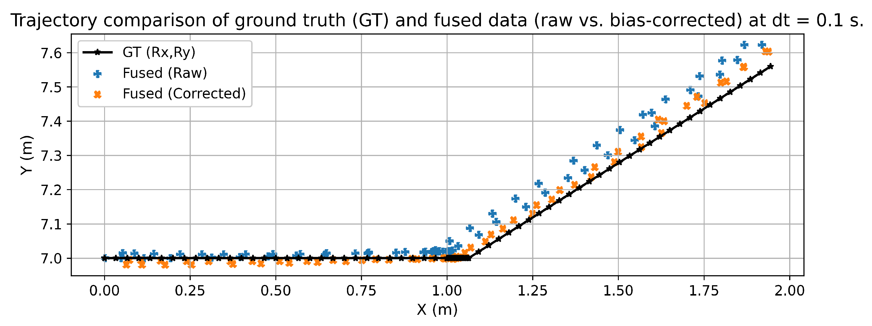
Figure 8.
Trajectory comparison between the ground truth (GT) and fused data (raw and bias-corrected) at s.
Figure 8.
Trajectory comparison between the ground truth (GT) and fused data (raw and bias-corrected) at s.
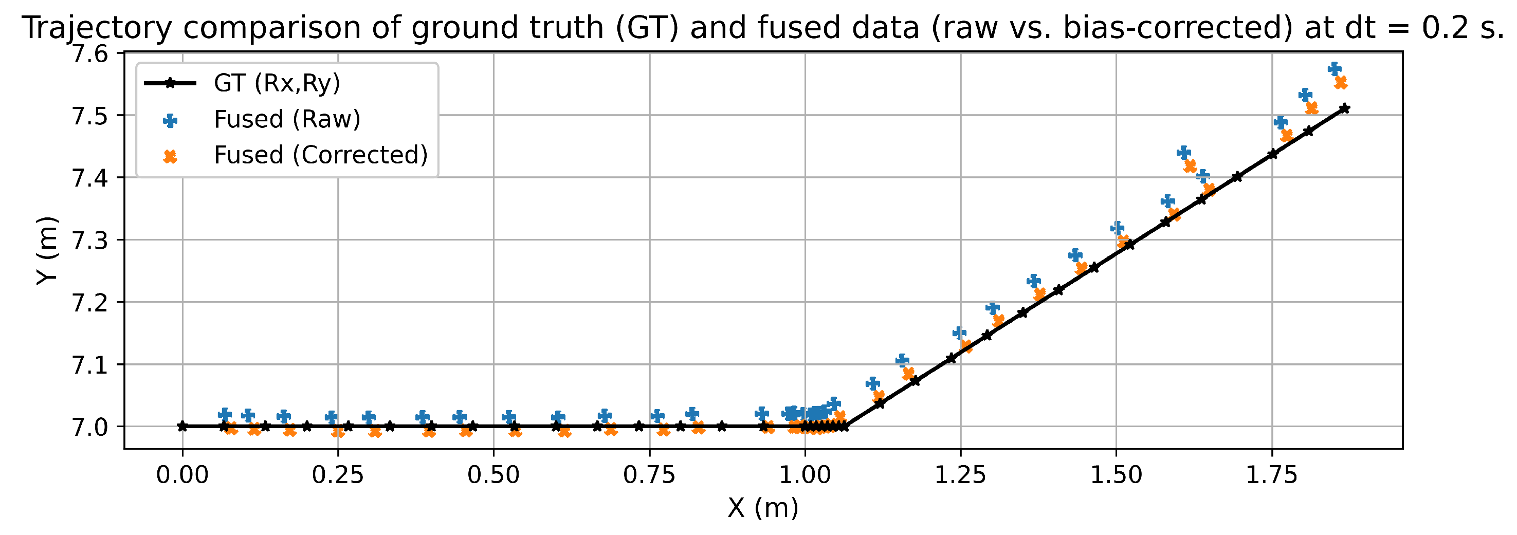
Figure 9.
Trajectory comparison between the normal and blended Extended Kalman Filter (EKF) models at s.
Figure 9.
Trajectory comparison between the normal and blended Extended Kalman Filter (EKF) models at s.
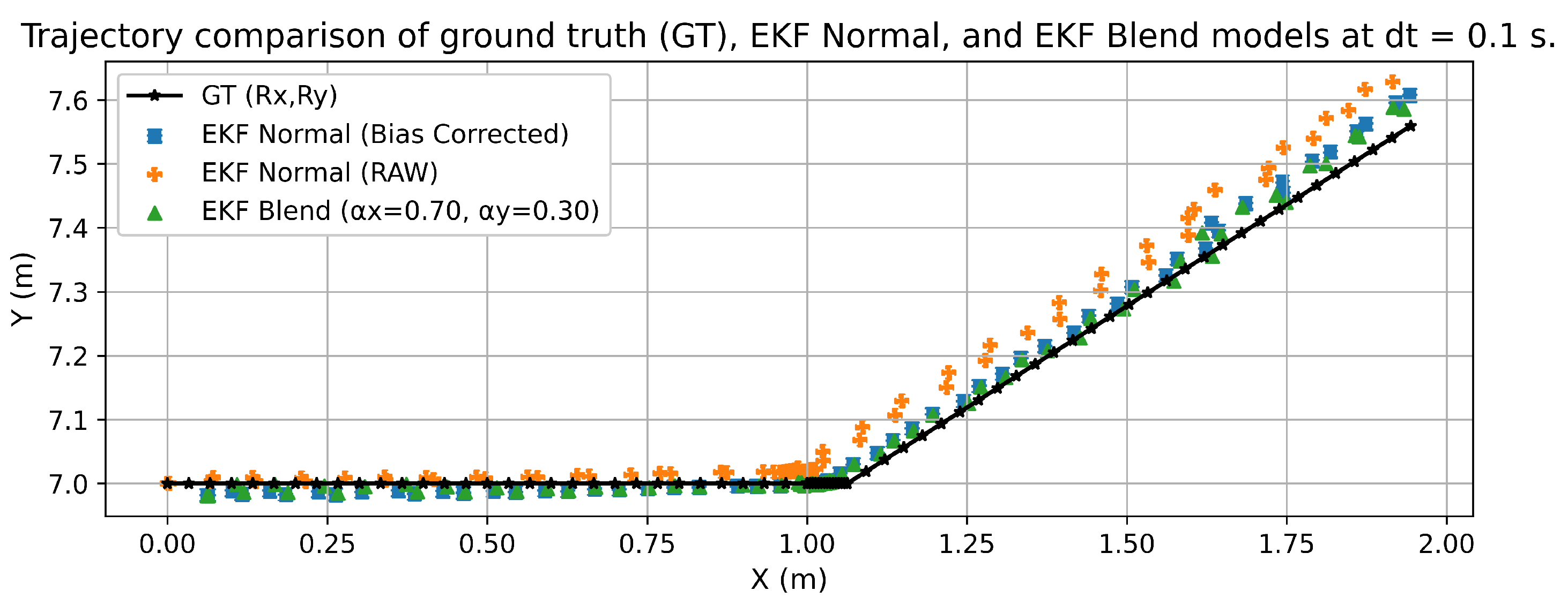
Figure 10.
Trajectory comparison between the normal and blended Extended Kalman Filter (EKF) models at s.
Figure 10.
Trajectory comparison between the normal and blended Extended Kalman Filter (EKF) models at s.
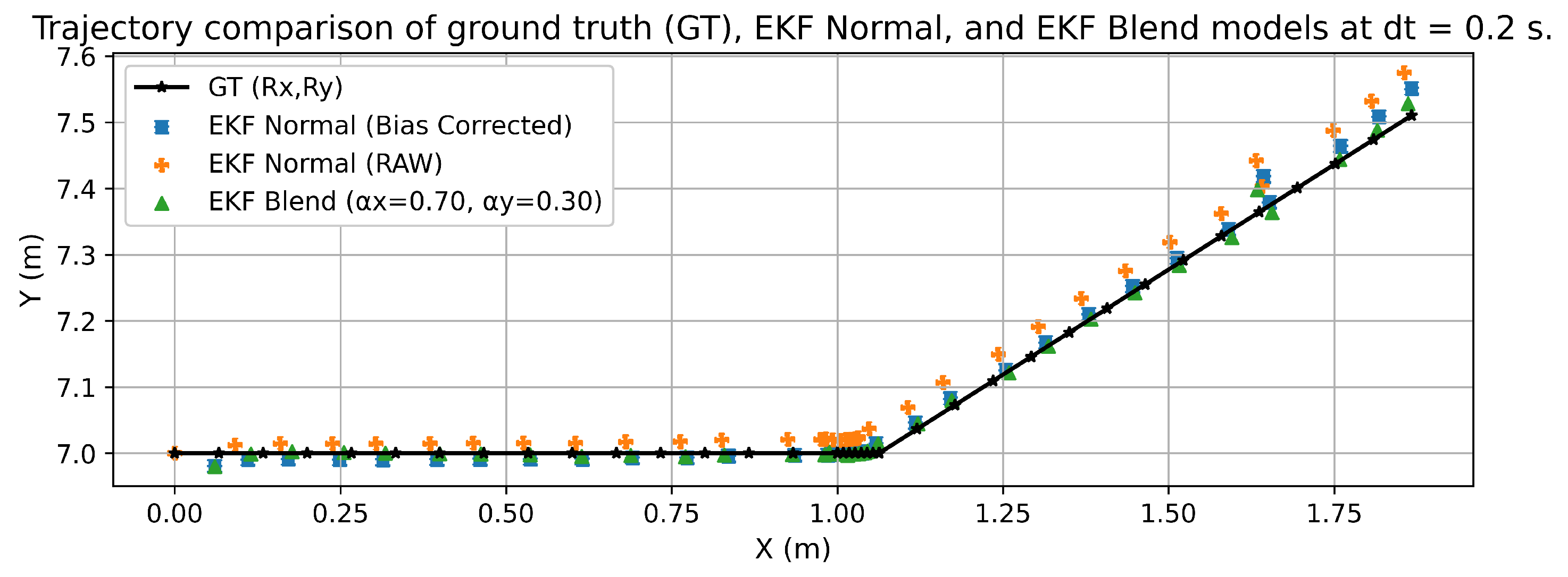

Table 1.
Summary of sensor specifications used in the AGV localization system.
| Sensor | Model | Specifications |
|---|---|---|
| Encoder | DC Motor JGB37-520 with Double Magnetic Hall Encoder | AB-phase (quadrature) output for direction and revolution detection; 90 pulses/rev; operating voltage: 3.3–5 V DC. |
| IMU | WitMotion WT901C (9-DOF) | Measures linear acceleration ( g), angular velocity (/s), and orientation; sampling rate: 10 Hz. |
| CCTV | TP-Link Tapo C200 | Wireless IP camera; 1080p at 30 fps; H.264 compression; IR LED (850 nm, up to 30 ft); WiFi video streaming. |
| Reference Camera (GT) | OKER HD-869 | Full HD (1920×1080) resolution; auto-focus lens; used as the ground-truth reference camera. |
Table 2.
Average bias errors of each sensor at different sampling intervals.
| Sampling interval (s) | Sensor | Mean Error X (m) | Mean Error Y (m) | Mean Error (rad) |
|---|---|---|---|---|
| 0.1 | CAM | 0.0305 | 0.0268 | – |
| DR | -0.0617 | 0.0190 | – | |
| IMU | – | – | 0.0977 | |
| 0.2 | CAM | 0.0250 | 0.0290 | – |
| DR | -0.0604 | 0.0201 | – | |
| IMU | – | – | 0.1006 |
The symbol “–” indicates that no measurement or estimation is available for that axis.
Table 3.
Root mean square error (RMSE) values of the sensors before (raw) and after bias correction (BC) at two sampling intervals ( s and s).
Table 3.
Root mean square error (RMSE) values of the sensors before (raw) and after bias correction (BC) at two sampling intervals ( s and s).
| Sampling interval (s) | Sensor | X Raw (m) | X BC (m) | Y Raw (m) | Y BC (m) | Raw (rad) | BC (rad) |
|---|---|---|---|---|---|---|---|
| 0.1 | CAM | 0.0617 | 0.0536 | 0.0467 | 0.0382 | – | – |
| DR | 0.0792 | 0.0497 | 0.0241 | 0.0148 | – | – | |
| IMU | – | – | – | – | 0.2256 | 0.2018 | |
| 0.2 | CAM | 0.0483 | 0.0414 | 0.0459 | 0.0355 | – | – |
| DR | 0.0780 | 0.0495 | 0.0255 | 0.0157 | – | – | |
| IMU | – | – | – | – | 0.2317 | 0.2072 |
“–” indicates that no measurement or estimation is available for that axis.
Table 4.
Variance and corresponding weights of CAM, DR, and IMU sensors at s.
| Data type | Sensor | Var X (m2) | Var Y (m2) | Var (rad2) | |||
|---|---|---|---|---|---|---|---|
| Raw | CAM | 0.002904 | 0.001478 | – | 0.460989 | 0.129245 | – |
| DR | 0.002483 | 0.000219 | – | 0.539011 | 0.870755 | – | |
| IMU | – | – | 0.041277 | – | – | 1.000000 | |
| Bias corrected | CAM | 0.002904 | 0.001478 | – | 0.460989 | 0.129245 | – |
| DR | 0.002483 | 0.000219 | – | 0.539011 | 0.870755 | – | |
| IMU | – | – | 0.041277 | – | – | 1.000000 |
The symbol “–” indicates that no measurement or estimation is available for that axis.
Table 5.
Variance and corresponding weights of CAM, DR, and IMU sensors at s.
| Data type | Sensor | Var X (m2) | Var Y (m2) | Var (rad2) | |||
|---|---|---|---|---|---|---|---|
| Raw | CAM | 0.001732 | 0.001278 | – | 0.588462 | 0.164134 | – |
| DR | 0.002477 | 0.000251 | – | 0.411538 | 0.835866 | – | |
| IMU | – | – | 0.044070 | – | – | 1.000000 | |
| Bias corrected | CAM | 0.001732 | 0.001278 | – | 0.588462 | 0.164134 | – |
| DR | 0.002477 | 0.000251 | – | 0.411538 | 0.835866 | – | |
| IMU | – | – | 0.044070 | – | – | 1.000000 |
The symbol “–” indicates that no measurement or estimation is available for that axis.
Table 6.
Summary of RMSE values for fused data before and after bias correction at two different sampling intervals.
Table 6.
Summary of RMSE values for fused data before and after bias correction at two different sampling intervals.
| Sampling interval (s) | Fusion type | RMSE X (m) | RMSE Y (m) |
|---|---|---|---|
| 0.1 | Fused (Raw) | 0.0661 | 0.0230 |
| Fused (Corrected) | 0.0483 | 0.0122 | |
| 0.2 | Fused (Raw) | 0.0415 | 0.0235 |
| Fused (Corrected) | 0.0402 | 0.0095 |
The root mean square error (RMSE) values represent the deviation of fused trajectories from the ground truth (GT) in the X and Y directions. “Corrected” indicates data after bias removal, while “Raw” refers to uncorrected data.
Table 7.
Summary of root mean square error (RMSE) values for Extended Kalman Filter (EKF) models at two sampling intervals ( s and s).
Table 7.
Summary of root mean square error (RMSE) values for Extended Kalman Filter (EKF) models at two sampling intervals ( s and s).
| Sampling interval (s) | EKF model | RMSE X (m) | RMSE Y (m) | RMSE XY (m) |
|---|---|---|---|---|
| 0.1 | Normal (Raw) | 0.060541 | 0.022919 | 0.064734 |
| Normal (Bias Corrected) | 0.047174 | 0.012047 | 0.048688 | |
| Blend () | 0.047108 | 0.009638 | 0.048084 | |
| Blend () | 0.047699 | 0.009897 | 0.048715 | |
| Blend () | 0.047114 | 0.009983 | 0.048160 | |
| Blend () | 0.047696 | 0.009983 | 0.048729 | |
| Blend () | 0.047118 | 0.009897 | 0.048146 | |
| 0.2 | Normal (Raw) | 0.040356 | 0.023574 | 0.046737 |
| Normal (Bias Corrected) | 0.039453 | 0.009881 | 0.040672 | |
| Blend () | 0.040282 | 0.011603 | 0.041920 | |
| Blend () | 0.043155 | 0.007732 | 0.043842 | |
| Blend () | 0.038740 | 0.018405 | 0.042889 | |
| Blend () | 0.043131 | 0.018432 | 0.046905 | |
| Blend () | 0.038761 | 0.007731 | 0.039524 |
RMSE values are rounded to six decimal places for consistency. Boldface entries can be added to highlight the lowest RMSE values for each case.
Disclaimer/Publisher’s Note: The statements, opinions and data contained in all publications are solely those of the individual author(s) and contributor(s) and not of MDPI and/or the editor(s). MDPI and/or the editor(s) disclaim responsibility for any injury to people or property resulting from any ideas, methods, instructions or products referred to in the content. |
© 2025 by the authors. Licensee MDPI, Basel, Switzerland. This article is an open access article distributed under the terms and conditions of the Creative Commons Attribution (CC BY) license (http://creativecommons.org/licenses/by/4.0/).
Copyright: This open access article is published under a Creative Commons CC BY 4.0 license, which permit the free download, distribution, and reuse, provided that the author and preprint are cited in any reuse.


