Machine Learning-Based Approaches for Solar Energy Forecasting

I. Introduction

II. Feature Enginnerin in Solar Forecasting

III. Machine Learning Models

B. Ridge Regression

In the realm of ordinaiy multiple linear regression, a set of p predictor variables collaborates with a response variable to formulate a model in the structure of:

Y =Bo-:- fhX1 + r)2X2 + ··” + BpXp + £

Unpacking the terminology:

-

Y denotes the response variable.

-

XJ stands for the jth predictor variable.

-

p j represents the average influence on Y when a one-unit increase is observed in XJ, \vhile keeping other predictors constant”

-

i.:: represents the eITor term.

To compute the values of po, Bi, f.:b, .. _, BP, the least squares method comes into play, aiming to rninirnize the summation of squared residuals (RSS):

Breaking down the fbrmula:

-

:E signifies the sunm1ation operation.

-

Yi represents the actual response value for the ith observation.

-

Yi symbolizes the predicted response value generated by the multiple linear regression model.

However, the situation becomes intricate when predictor variables showcase significant correlation, vvhich leads to the emergence of multicollinearity. This phenomenon can render the coefficient estimates of the model unstable, introducing a high degree of variability.

To address this challenge without entirely discarding particular predictor variables, an alternative technique known as ridge regression comes into play. Ridge regression embarks on the task of minimizing the ensuing expresswn:

Here:

-

j ranges from 1 to p.

-

I, (lambda) assumes a non-negative value.

The supplementary term vvithin the equation is tenned a “shrinkage penalty.’’ When ;, equals 0, this penalty component holds no sway, causing ridge regression to yield coefficient estimates akin to those of the least squares approach. However, as ’A, ascends towards infinity, the influence of the shrinkage penalty gains prominence, compelling the coefficient estimates of ridge regression to gradually approach zero.

Tn practical application, predictor variables bearing lesser influence on the model tend to converge towards zero at an accelerated rate due to the intrinsic shrinkage impact.

C. Lasso Regression

ln the context of ordinary multiple linear regression, a collection of p predictor variables and a response variable combine to constrnct a model characterized by the equation:

Y = Bo+ B1X1 + B,X2 + ... + BpXp + S

The key elements in this equation are:

-

Y: Represents the response variable.

-

XJ: Denotes the jth predictor variable.

-

f3j: Signifies the average impact on Y resulting from a one-unit increase in Xj, keeping aU other predictors constant.

-

s: Stands for the error term.

The values of Po, f31, Pz, “ .., f\1 are determined through the utilization of the least squares method, which aims to minimize the sum of squared residuals (RSS):

RSS = I{yi - 5\)2

In this equation:

-

I: represents the summation symbol.

-

Yi signifies the actual response value for the ith observation.

-

Yi stands fiff the predicted response value derived from the multiple linear regression model.

However, situations arise where predictor variables exhibit strnng correlation, leading to the emergence of multicollinearity. This phenmnenon can result in unreliable coefficient estirnates for the model, with an increased potential for high variance. In essence, when the model is applied to new, previously unseen data, its performance is likely to be suhpar.

One approach to address this challenge is by employing lasso regression, which endeavors to minimize the foUowing expression:

Here:

-

j ranges from 1 to p.

-

I, (lambda) assumes a non-negative value.

The additional term within the equation is referred to as a “shrinkage penalty.’° vVhen ;.., equals 0, this penalty term holds no impact, rendering lasso regression equivalent to the coefficient estimates obtained through the least squares method.

However, as ““ progressively increases towards infinity, the influence of the shrinkage penalty intensifies. Consequently, predictor variables deemed less significant in the model experience a substantial shrinkage effect, moving them towards zero. In certain cases, some predictor variables might even be eliminated from the _model entirely.

D. Decision Tree Regression

The term “decision tree” aptly reflects its operational principle based on conditions. This method boasts efficiency and employs robust algorithms for predictive analysis. It comprises fundamental components: internal nodes, branches, and terminal nodes. In the context of a decision tree, each internal node conducts a “test” on an attribute, with branches indicating the outcomes of these tests, while every leaf node signifies a class label. Its versatility is evident as it caters to both classification and regression tasks, constituting two essential types of supervised learning algorithms. However, the sensitivity of decision trees to their training data is noteworthy - even minor alterations in the training set can lead to significant variations in the resulting tree structures.

Certainly, let’s delve into the intuition and mathematical theory behind Decision Tree Regression (DTR). Intuition:

Think of a decision tree as a series of questions that help you arrive at a decision. In the context of regression, the goal is to predict a continuous output value for a given set of input features. Each internal node of the tree poses a question based on a specific feature, and depending on the answer, you move to one of the child nodes. The leaf nodes provide the predicted output values.

Mathematical Theory:

At each internal node, the algorithm chooses the feature and threshold that best splits the data into subsets. The splitting is determined by a criterion that aims to minimize the variance (or another suitable measure) of the target values within each subset. In the case of regression, a common splitting criterion is to minimize the mean squared error (MSE), which can be defined as follows for a given node N:

[ MSE(N) = \frac{l}{INI} \sum_{i \in N} (y_i- \bar{y}_N)l’2]

Here, \( y_i \) represents the target value of the i-th data point in node N, and \( \bar{y}_N \) is the mean of the target values in node N.

2. [“l/i>fff..: r· rfli {:,3

When a leaf node is created, it’s assigned a constant value that represents the prediction for all data points falling into that leaf For regression, this value is typically the average (or median) of the target values within the leaf

The process of building a decision tree is recursive. Starting from the root node, the algorithm selects the best feature and threshold for splitting the data. Then, it moves to the child nodes and repeats the process until a stopping criterion is met (e.g., maximum tree depth, minimum number of samples per leaf).

Decision trees have a tendency to overfit the training data if they become too deep. Overfitting refers to the model capturing noise in the data instead of the underlying patterns. Pruning is a technique to address this by removing or collapsing nodes that do not contribute significantly to the model’s performance on validation data.

IV. Ensemble Learning Models

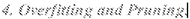
A. Random Forest

Random forest, as its name suggests, comprises an enormous amount of individual decision trees that work as a group or as they say, an ensemble. Every individual decision tree in the random forest lets out a class prediction and the class with the most votes is considered as the model’s prediction.

Random forest uses this by permitting every individual tree to randomly sample from the dataset with replacement, bringing about various trees. This is known as bagging.Random Forest has multiple decision trees as base learning models. We randomly perform row sampling and feature sampling from the dataset forming sample datasets for every model. This part is called Bootstrap.

Assumptions.for Random Forest

Since the random forest combines multiple trees to predict the class of the dataset, it is possible that some decision trees may predict the correct output, while others may not. But together, all the trees predict the correct output. Therefore, below are two assumptions for a better Random forest classifier:

• There should be some actual values in the feature variable of the dataset so that the classifier can predict accurate results rather than a guessed result.
• The predictions from each tree must have very low correlations.

Why use Random Forest?

Below are some points that explain why we should use the Random Forest algorithm:

• It takes less training time as compared to other algorithms.
• It predicts output with high accuracy, even for the large dataset
• It runs efficiently.It can also maintain accuracy when a large proportion of data is missing.

How does Random Forest algorithm work?

Random Forest works in two-phase first is to create the random forest by combining N decision tree, and second is to make predictions for each tree created in the first phase.

The Working process can be explained in the below steps and diagram:

Step-1: Select random K data points from the training set.

Step-2: Build the decision trees associated with the selected data points (Subsets).

Step-3: Choose the number N for decision trees that you want to build.

Step-4: Repeat Step I & 2.

Step-5: For new data points, find the predictions of each decision tree, and assign the new data points to the category that wins the majority votes.

Figure 1. Random Forest Regression Model.

Figure 1. Random Forest Regression Model.

D. Gradient Boosting Regressor

Gradient Boosting is a robust boosting algorithm that fuses weak learners into potent ones by minimizing a loss function, such as mean squared error or cross-entropy, of the preceding model’s predictions using gradient descent. In each iteration, it calculates the gradient of the loss function concerning the current ensemble’s predictions and then trains a new weak model to minimize this gradient. The new model’s predictions are integrated into the ensemble, and this cycle continues until a stopping condition is met.

In contrast to AdaBoost, Gradient Boosting doesn’t modify training instance weights. Instead, it trains each predictor using the residual errors from the previous one as labels. A technique called Gradient Boosted Trees employs a base learner like CART (Classification and Regression Trees). The process is illustrated in Figure 2.13, where an ensemble of M trees is trained. Tree l is created using feature matrix X and labels y. The predictions yl(hat) help compute the residual errors r1. Tree2 is trained using X and the r1 residuals as labels. The process repeats for all M trees.

A significant parameter in this method is the “Shrinkage,” where the prediction of each tree is scaled after being multiplied by the learning rate (eta) within the range of Oto 1. Balancing eta and the number of estimators is vital reducing the learning rate should be compensated by increasing estimators to maintain model performance.

The Gradient Boosting Algorithm’s steps are as follows:

Stq-,: ] :Given input X and target Y with N samples, aim to learn the function f(x) that maps X to y. Boosted trees comprise the sum of trees. The loss function quantifies the discrepancy between actual and predicted values.

Sk:p 2:The objective is to minimize the loss function L(f) with respect to f

J: Steepest Descent:For M-stage gradient boosting, steepest descent identifies where is a constant step length, and gim is the gradient of loss function L(f).

Gradient Boosting Regressor (GBR) is a widely used machine learning algorithm that merges weak predictive models, usually decision trees, to create a robust predictive model. Here are advantages and disadvantages of employing Gradient Boosting Regressor.

V. Performance Metrics

VI. Dataset Information

VII. Results and Discussion

A. Machine Learning Models

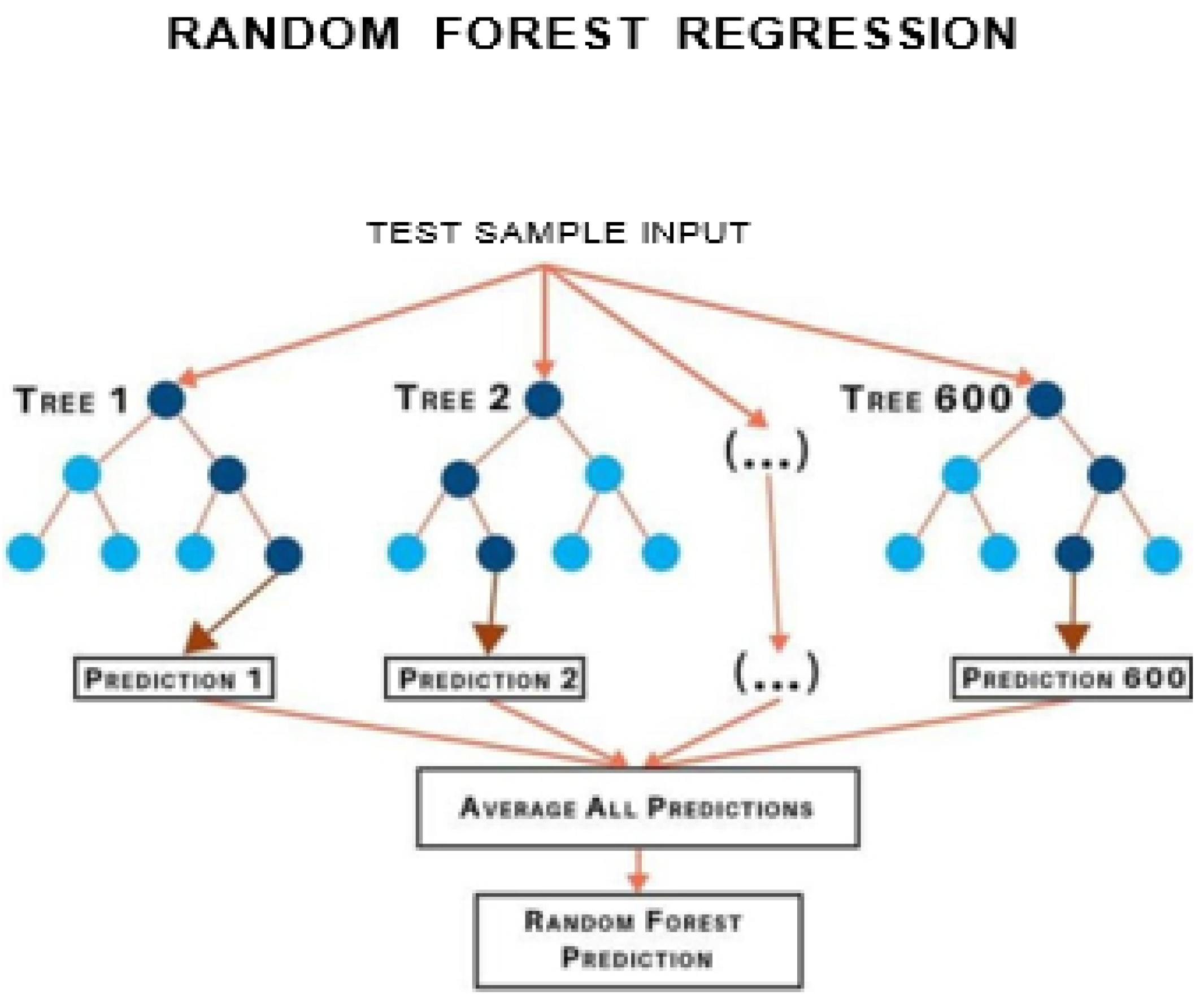
The machine learning models employed in this study involved creating simple forecasts based on the assumption of slow changes or persistence in daily solar PV power production. As a result of these simplistic assumptions, the performance of these models was not anticipated to be highly accurate. This observation is evident from the outcomes presented in figure-2,3,4,5 depicting the Mean Square Error(MSE), Root Mean Square Error (RMSE), Mean Absolute Error(MAE) and the Coefficient ofDetermination(W’2) for model evaluations.

The MSE is the average of the squared differences between predicted and actual values. It’s a measure of the average magnitude of prediction errors. A lower MSE is preferable, indicating that the algorithm’s predictions are closer to the actual values. In the hypothetical comparison, Decision Tree Regression(DTR) demonstrates the best performance with the lowest MSE, indicating that its predictions have the smallest squared errors on average. Decision Tree Regression, with the highest MSE, has predictions with larger squared errors on average.

Figure 2. MSE comparison of Machine Learning models.

Figure 2. MSE comparison of Machine Learning models.

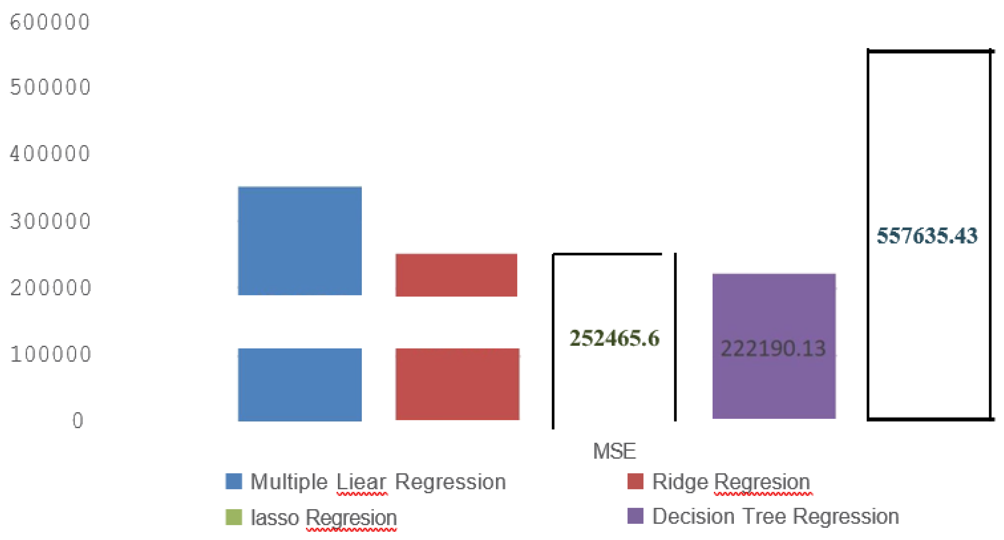
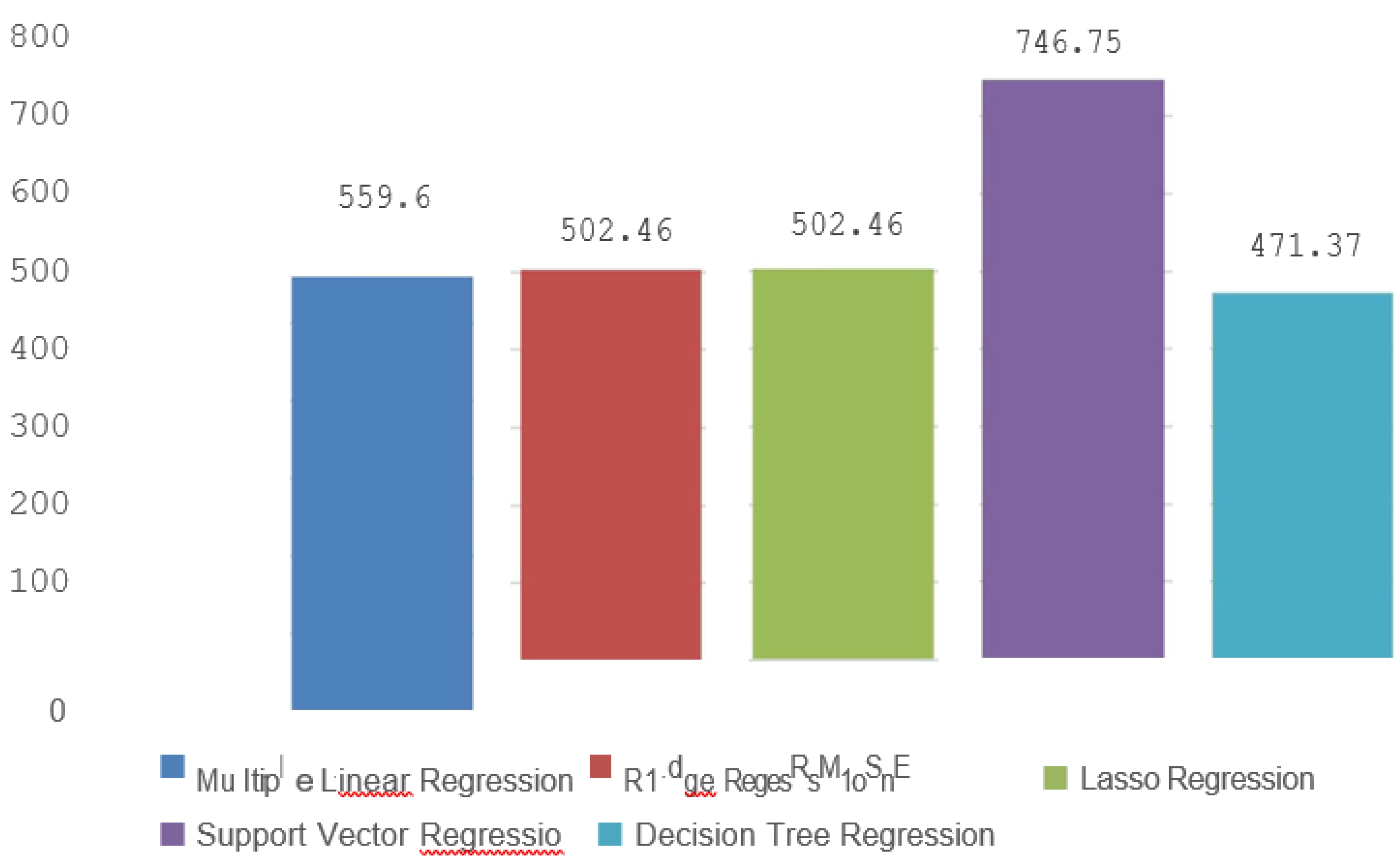
The RMSE is a widely-used metric that represents the square root of the average squared differences between predicted and actual values. A lower RMSE indicates better predictive accuracy, as it signifies that the algorithm’s predictions are closer to the true values. In the hypothetical comparison, Decision Tree Regression(DTR) has the lowest RMSE, suggesting that it is able to capture the data’s variations more accurately than the other algorithms. On the other hand, Support Vector Regression(SVR) has the highest RMSE, suggesting that its predictions exhibit more variability from the actual values.

Figure 3. RMSE comparision of Machine Learning modes.

Figure 3. RMSE comparision of Machine Learning modes.

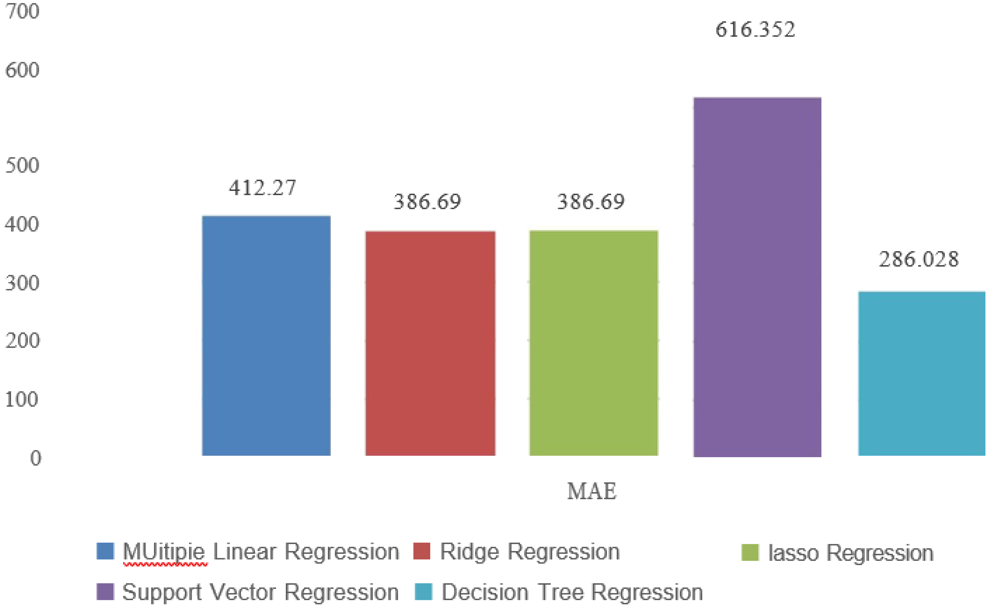
The MAE measures the average absolute differences between predicted and actual values. Unlike squared error metrics, MAE gives equal weight to all errors regardless of their magnitude. A lower MAE suggests better predictive accuracy. In our comparison, Decision Tree Regression(DTR) has the lowest MAE, indicating that its predictions are, on average, closer to the true values compared to the other algorithms. Support Vector Regression has the highest MAE, implying that its predictions deviate more in terms of absolute value.

Figure 4. MAE comparison of Machine Leaming models.

Figure 4. MAE comparison of Machine Leaming models.

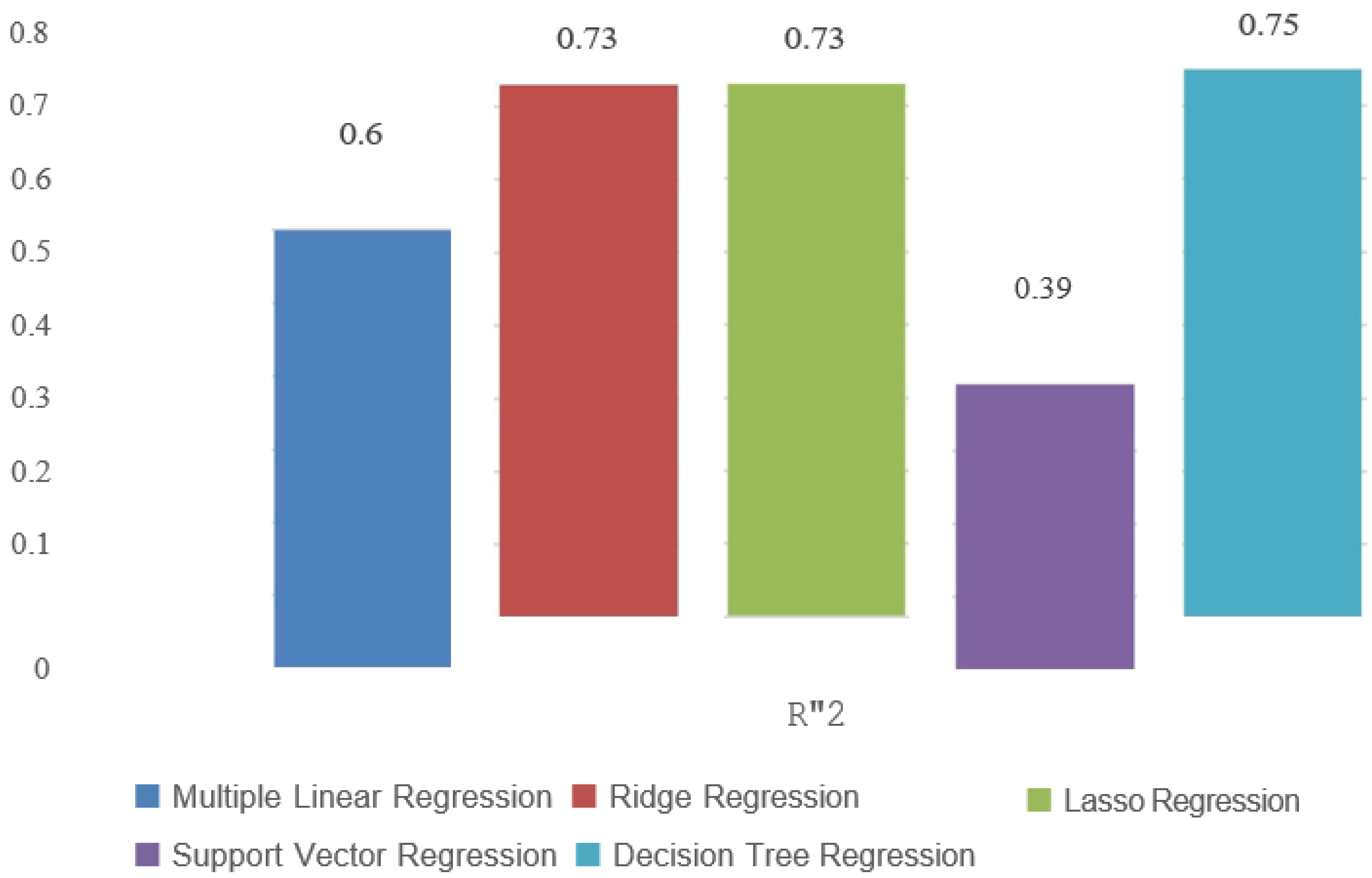
The R-squared represents the proportion of the variance in the dependent variable that is predictable from the independent variables. A higher R-squared value indicates a better fit of the model to the data. In the hypothetical comparison, SVR has the highest R-squared value, suggesting that it explains a larger proportion of the variance in the target variable compared to the other algorithms. This indicates that the Decision Tree Regression(DTR) model captures more of the underlying relationships within the data. Conversely, Support Vector Regression(SVR) has the lowest R-squared, implying that it might not be capturing the complex patterns present in the data as effectively as the other algorithms.

Figure 5. W’2 comparison of Machine Learning Models.

Figure 5. W’2 comparison of Machine Learning Models.

In this hypothetical scenario, we can observe that:

-

Decision Tree Regression(DTR) has the lowest RMSE, MSE, and MAE values, indicating better predictive accuracy compared to other algorithms.

-

MLR, Ridge, and Lasso have fairly similar performance in terms ofRMSE, MSE, and MAE, with Ridge slightly outperforming Lasso.

-

Support Vector Regression(SVR) has higher RMSE, MSE, and MAE values, indicating that it might not be capturing the underlying patterns as effectively as the linear-based methods or SVR.

-

Decision Tree Regression also has the highest R-squared value, implying a better fit to the data compared to other algorithms.

In summary, the choice of regression algorithm depends on the specific trade-offs you want to make between accuracy, interpretability, and complexity. Decision Tree Regression(DTR) seems to perform well in this hypothetical scenario across all metrics, indicating a balance between accurate prediction and model fit. However, it’s important to validate these findings on real-world data and consider other factors such as model interpretability and computational complexity before making a final decision.

B. Ensemble Learning Models

Ensemble methods in machine learning consistently outperform individual ML models, showcasing their remarkable ability to enhance predictive capabilities. These techniques harness the collective intelligence of diverse models, resulting in a significant boost in accuracy and a deeper understanding ofintricate data relationships. The synergy achieved through ensemble methods enables them to effectively navigate complex patterns that might elude standalone models.

Consequently, ensemble techniques stand as a formidable approach in elevating the performance and reliability of predictive modeling, showcasing their superiority in the realm of machine learning.As a result of these simplistic assumptions, the performance ofthese models was not anticipated to be highly accurate. This observation is evident from the outcomes presented in figure-6,7,8,9 depicting the Mean Square Error(MSE), Root Mean Square Error (RMSE), Mean Absolute Error(MAE) and the Coefficient ofDetermination(W’2) for model evaluations.

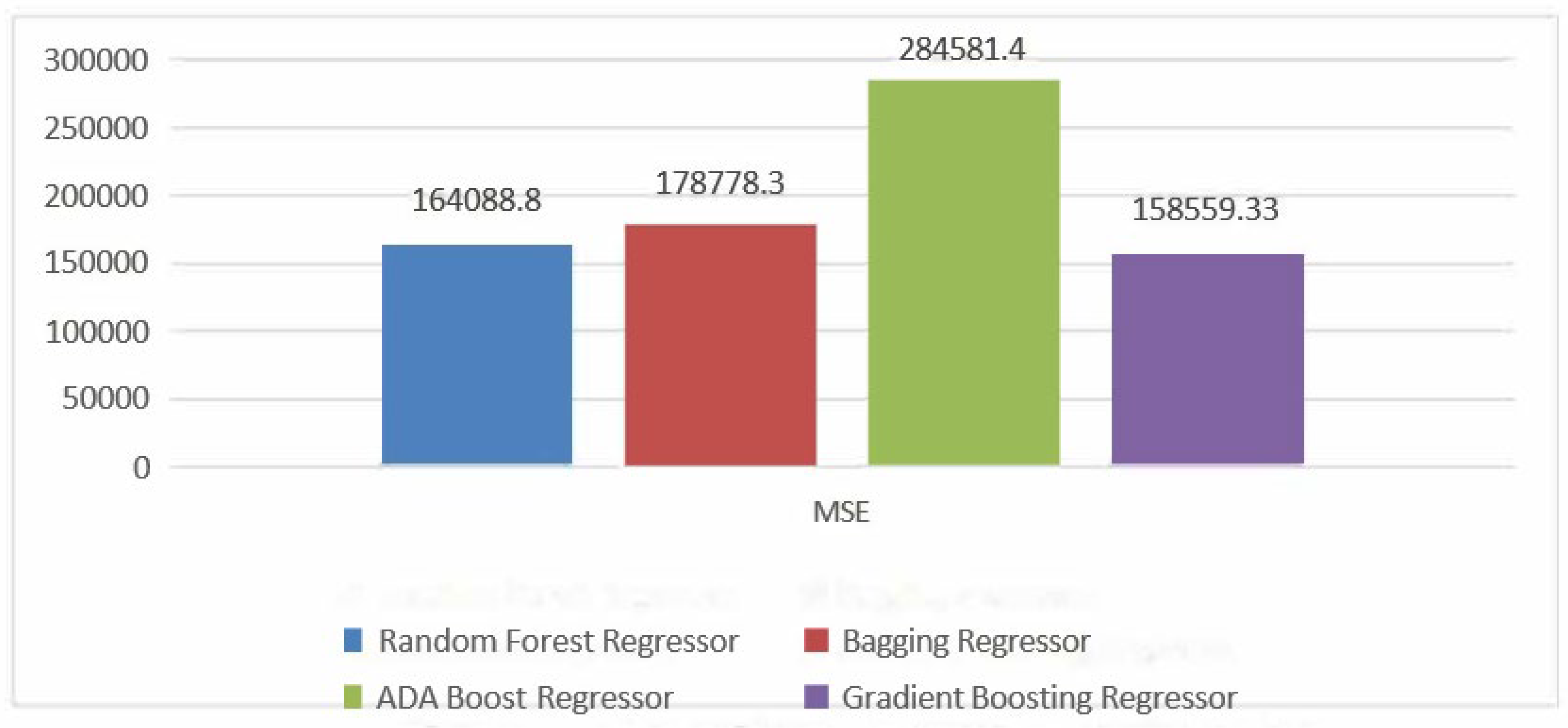
The MSE is the average ofthe squared differences between predicted and actual values. It’s a measure ofthe average magnitude ofprediction errors. A lower MSE is preferable, indicating that the algorithm’s predictions are closer to the actual values. In the hypothetical comparison from figure-6, Gradient Boostig Regressor(GBR) demonstrates the best performance with the lowest MSE, indicating that its predictions have the smallest squared errors on average. ADA Boost Regressor, with the highest MSE, has predictions with larger squared errors on average.

Figure 6. MSE comparision ofEnsemble Learning models.

Figure 6. MSE comparision ofEnsemble Learning models.

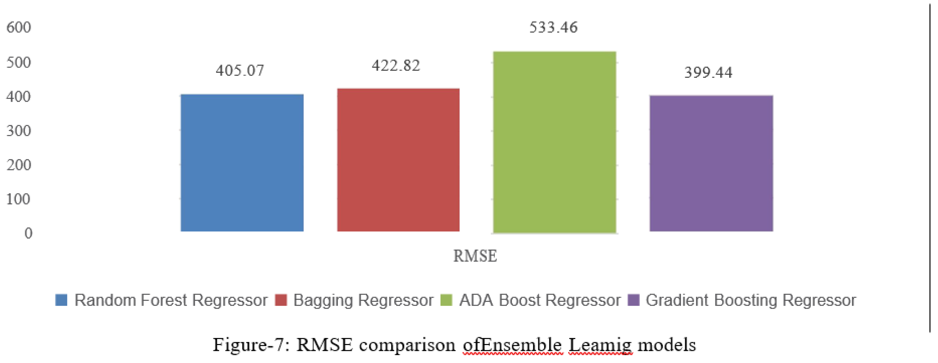
RMSE is a widely-used metric that represents the square root ofthe average squared differences between predicted and actual values. A lower RMSE indicates better predictive accuracy, as it signifies that the algorithm’s predictions are closer to the true values. In the hypothetical comparison from figure-7, Gradient Boosting Regressor has the lowest RMSE, suggesting that it is able to capture the data variations more accurately than the other algorithms. On the other hand, ADA Boost Regressor has the highest RMSE, suggesting that its predictions exhibit more variability from the actual values.

Figure 7. RMSE comparison ofEnsemble Leamig models.

Figure 7. RMSE comparison ofEnsemble Leamig models.

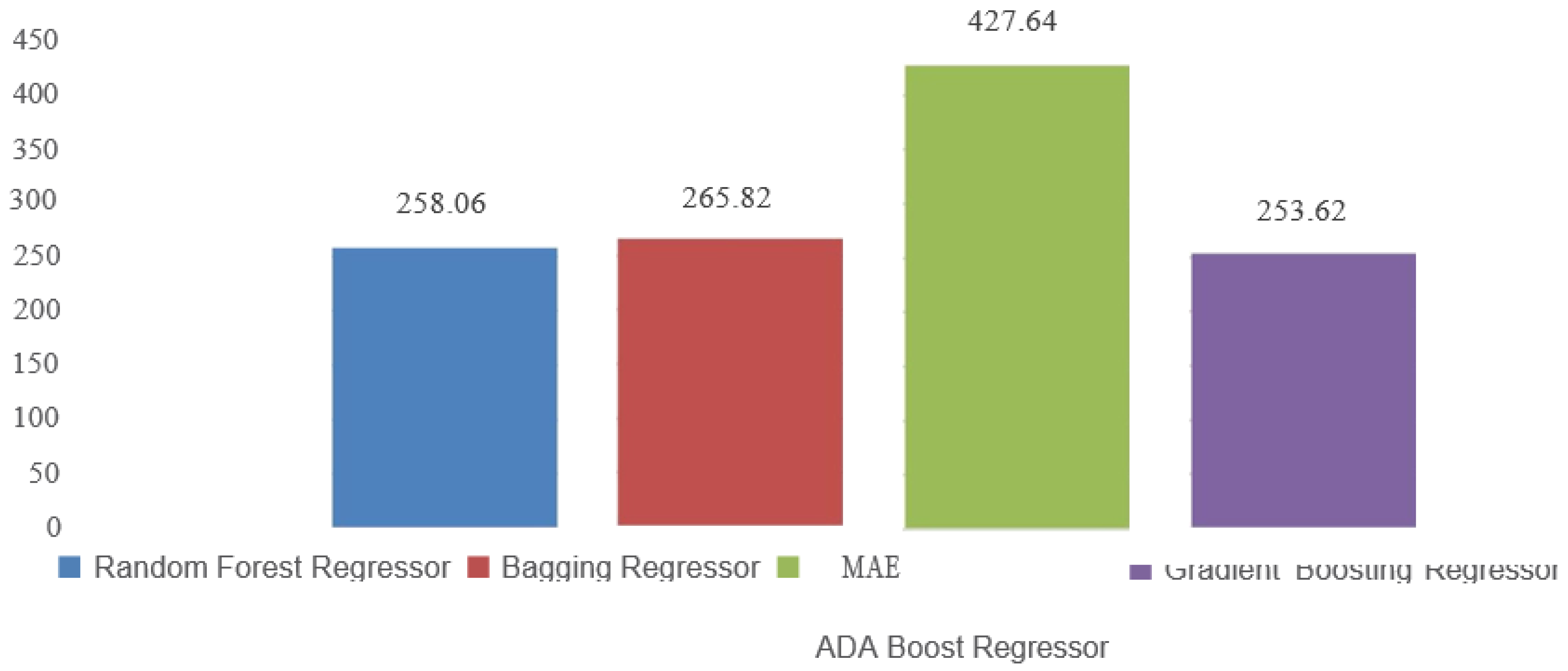
MAE measures the average absolute differences between predicted and actual values. Unlike squared error metrics, MAE gives equal weight to all errors regardless of their magnitude. A lower MAE suggests better predictive accuracy. In our comparison from figure-8, Gradient Boosting Regressor has the lowest MAE, indicating that its predictions are, on average, closer to the true values compared to the other algorithms. ADA Boost Regressor has the highest MAE, implying that its predictions deviate more in terms of absolute value.

Figure 8. MAE comparision of Ensemble Leaming models.

Figure 8. MAE comparision of Ensemble Leaming models.

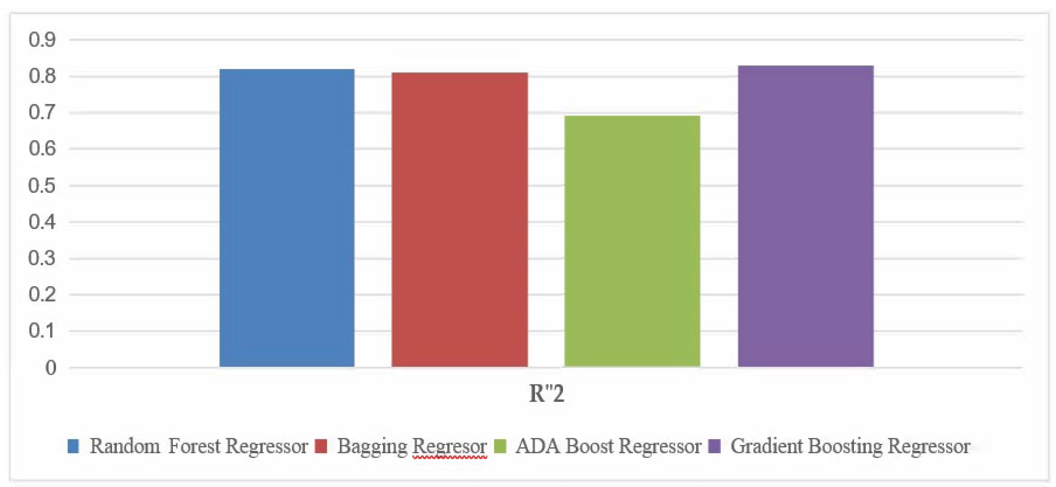
R-squared represents the proportion of the variance in the dependent variable that is predictable from the independent variables. A higher R-squared value indicates a better fit of the model to the data. In the hypothetical comparison, SVR has the highest R-squared value, suggesting that it explains a larger proportion of the variance in the target variable compared to the other algorithms. This indicates that the SVR model captures more of the underlying relationships within the data. Conversely, Decision Tree Regression has the lowest R-squared, implying that it might not be capturing the complex patterns present in the data as effectively as the other algorithms.

Figure 9. W’2 comparision ofEnsemble Learning Models.

Figure 9. W’2 comparision ofEnsemble Learning Models.

In this hypothetical scenario, we can observe that:

-

Gradient Boosting Regressor has the lowest RMSE, MSE, and MAE values, indicating better predictive accuracy compared to other algorithms.

-

ADA Boost Regressor has higher RMSE, MSE, and MAE values, indicating that it might not be capturing the underlying patterns as effectively as the linear-based methods or SVR.

-

Gradient Boostig Regressor also has the highest R-squared value, implying a better fit to the data compared to other algorithms.

In summary, the choice of regression algorithm depends on the specific trade-offs you want to make between accuracy, interpretability, and complexity. Decision Tree Regression(DTR) seems to perform well in this hypothetical scenario across all metrics, indicating a balance between accurate prediction and model fit. However, it’s important to validate these findings on real-world data and consider other factors such as model interpretability and computational complexity before making a final decision.

Comparison

In this section we will compare all performance metrics from the results section. In given below table all the machine learning and ensemble model performance metrics are compared and best method is concluded based on the the Mean Square Error(MSE), Root Mean Square Error (RMSE), Mean Absolute Error(MAE) and the Coefficient ofDetermination(W’2) for model evaluations.

Table 2. comparison of performance metrics of machine learning and Ensemble Learning models.

Table 2. comparison of performance metrics of machine learning and Ensemble Learning models.

MODEL	MSE	RMSE	MAE	W’2
MULTIPLE LINEAR REGRESSION	352465.7	559.6	412.27	0.6
RIDGE REGRESSION	252465.6	502.46	386.69	0.73
LASSO REGRESSION	252465.6	502.46	386.69	0.73
SUPPORT VECTOR REGRESSION	557635.43	746.75	616.352	0.39
DECISION TREE REGRESSION	222190.13	471.370	286.028	0.75
RANDOM FOREST REGRESSION	164088.8	405.07	258.06	0.82
BAGGING REGRESSOR	178778.3	422.82	265.82	0.81
ADA BOOST REGRESSOR	284581.40	533.46	427.64	0.69
GRADIENT BOOSTING REGRESSOR	158559.33	399.44	253.62	0.83

From the table we can conclude that the ensemble models performed better compared to the normal machine learning methods from the Table 9.1 we can say that Gradient boosting regressor is best model for this data set because it has high R6/\2 value of 0.83 and low MSE,RMSE and MAE values of 158559.33, 399.4 and 253.62.

VIII. Conclusion

IX. Future Scope

References

1. waone Gaboitaolelwe, Adamu Murtala Zungeru, Abid Yahya,” Machine Learning Based Solar PhotovoltaicPower Forecasting: A Review and Comparison”. [CrossRef]
2. Rai, A. Srivastava, and K. C. Jana, “An empirical analysis of machine learning algorithms for solar power forecasting in a high dimensional uncertain environment,” IETE Tech. Rev., pp. 1-16, Nov. 2022. [CrossRef]
3. S. Ghazi and K. Ip, “The effect ofweather conditions on the efficiency ofPV panels in the southeast ofU.K.,” Renew. Energy, vol. 69, pp. 50-59, Sep. 2014. [CrossRef]
4. Sheth, K., & Patel, D. (2024). Comprehensive examination of solar panel design: A focus on thermal dynamics.
5. Smart Grid and Renewable Energy, 15(1). [CrossRef]
6. D. Yang, J. Kleissl, C. A. Gueymard, H. T. C. Pedro, and C. F. M. Coimbra, “History and trends in solar irradiance and PV power forecasting: A preliminary assessment and review using text mining,’’ Sol. Energy, vol. 168, pp. 60-101, Jul. 2018. [CrossRef]
7. S. Leva, A. Dolara, F. Grimaccia, M. Mussetta, and E. Ogliari, “Analysis and validation of 24 hours ahead neural network forecasting of photovoltaic output power,” Math. Comput. Simul., vol. 131, pp. 88-100, Jan. 2017. [CrossRef]
8. D. V. Pombo, H. W. Bindner, S. V. Spataru, P. E. S0rensen, and P. Bacher, “Increasing the accuracy of hourly multi-output solar power forecast with physics-informed machine learning,” Sensors, vol. 22, no. 3, p. 749, Jan. 2022. [CrossRef]
9. Nouri, H., Hodge, B.-M., & Karimzadeh “Solar Power Forecasting: A Review of State-of-the-Art Methodologies” (2020). [CrossRef]
10. Inman, R. H., & Pedro, H. T. C.”Machine Leaming for Solar Power Forecasting: A Comprehensive Review” (2020). [CrossRef]
11. Amjady, N., & Keynia, “An Overview of Solar Power Forecasting and Prediction Intervals” (2020).
12. Renewable and Sustainable Energy Reviews, 131, 110029. [CrossRef]
13. Aghaei, J., & Fotuhi-Firuzabad,”Short-Term Solar Power Forecasting Using Machine Leaming Techniques” (2020), Energy Reports, 6, 1738-1753. [CrossRef]
14. Sheth, K., & Patel, D. (2024). Strategic placement of charging stations for enhanced electric vehicle adoption in San Diego, California. Journal of Transportation Technologies, 14(1), Article 141005. [CrossRef]
15. Swami, G., Sheth, K., & Patel, D. (2024). PV capacity evaluation using ASTM E2848: Techniques for accuracy and reliability in bifacial systems. Smart Grid and Renewable Energy, 15(9), Article 159012. [CrossRef]