The Gravitational Force on Charges and the Electric Force on Masses, Two Extremely Weak Action-Reaction Pairs, and the Geometric-Mean Relations of the Fundamental Constants of Nature

1. Introduction

1.1. The Geometric Means of Physical Quantities and Constants of Nature

The significance of geometric-mean (G-M) averaging of physical quantities in obtaining diverse new quantities was recently explored in a cosmological setting [1] and in particle physics [2,3]. Evidently, nature uses this type of mean because, unlike the arithmetic or the harmonic averages, the G-M does not primarily favor the larger or the smaller quantity, respectively. So, it appears that the G-M of two or more quantities with dissimilar magnitudes is a ‘fair’ (or at least impartial) approach in defining new values irrespective of the different units they may carry.

As in the definition of Lie groups [4], two G-M elements can be constructed from two given quantities (not counting the reciprocals). By extension, four G-M elements can be constructed from three given quantities, and by induction, then $2^{n-1}$ G-M elements result from n distinct quantities (or $2^n$ including the reciprocals) (Ref. [5], p. 10, item 3.1.6). The G-Ms encountered in constants of nature present some typical examples [1,2,3]:

(a)

The speed of light c imposed by the vacuum is the G-M average of the reciprocals of the vacuum permittivity ${\epsilon }_0$ and the vacuum permeability ${\mu }_0$, viz.

$$c=\sqrt{{\epsilon }_0^{-1}{\mu }_0^{-1}},$$

(1)

whereas the other G-M defines the impedance of free space $Z_0=\sqrt{{\epsilon }_0^{-1}{\mu }_0}$ .

(b)

The Compton length $r_{\mathrm{c}}\equiv h/\left(m_{\mathrm{e}}c\right)$ (where h is the Planck constant and $m_{\mathrm{e}}$ is the electron mass) is the G-M average

$$r_{\mathrm{c}}=\sqrt{r_{\mathrm{e}}{r}_{\mathrm{b}}},$$

(2)

of the classical electron radius $r_{\mathrm{e}}=r_{\mathrm{c}}\mathsf{\alpha }$ and the Bohr radius $r_{\mathrm{b}}=r_{\mathrm{c}}/\mathsf{\alpha }$, both written here in terms of the fine-structure constant $\mathsf{\alpha }$ (defined here in terms of the elementary charge e [6] and the Planck constant h [2,7,8]):

$$\mathsf{\alpha }\equiv {\displaystyle \frac{e^2}{4\pi {\epsilon }_{0}hc}}={\displaystyle \frac{1}{861.022576}}.$$

(3)

(c)

Because of equation (2), the Compton length is also the G-M of the three well-known atomic length scales, viz.

$$r_{\mathrm{c}}=\sqrt[3]{r_{\mathrm{e}}{r}_{\mathrm{c}}{r}_{\mathrm{b}}}.$$

(4)

Another example of a G-M involving physical variables was recently found for the strength of the dipolar magnetic field $B_{★}$ on the surface $r=R_{★}$ of an accreting pulsar of mass $M_{★}$ in a high-mass X-ray binary system [9], viz.

$$B_{★}=\sqrt{\left(g_{★}{\Sigma }_{★}\right)|d{P}_{★}/dt|},$$

(5)

where $g_{★}=G{M}_{★}/R_{★}^2$ is the surface gravity (G is Newton’s constant) and ${\Sigma }_{★}=M_{★}/\left(4\pi R_{★}^2\right)$ is the surface density of the pulsar, whereas $d{P}_{★}/dt$ is the rate of change of the pulsar’s spin period. The parenthesis highlights the factor that depends on intrinsic pulsar properties, whereas the factor $|d{P}_{★}/dt|$ of the G-M depends on an external influence due to the accretion of matter (which is measured in observations and is utilized as a probe of the magnetic field of the pulsar).

The data analysis of X-ray binary pulsars was carried out with a (non)linear Kalman-filter (KF) technique [10,11,12,13] capable of measuring temporal correlations in the fluctuations of the fundamental observed variables (pulsar spin period, X-ray luminosity) and the KF-derived time-dependent quantities (mass inflow rate, Maxwell stress, magnetospheric radius, corotation radius, magnetic moment). The nonlinear KF also follows the time-dependent evolution of two internal frequencies called ${\beta }_1$ and ${\beta }_2$. In the simpler version of the so-called ‘linear KF’ that describes a system in dynamic spin equilibrium, these frequencies merge into one value called ${\gamma }_{\Omega }$, which appears also in the nonlinear case as a G-M [9], viz.

$${\gamma }_{\Omega }=\sqrt{{\beta }_1{\beta }_2}.$$

(6)

Besides the above examples, there are many other physics equations involving G-Ms of constant and variable quantities, thus G-M averaging is pervasive in nature. Furthermore, even the equations that do not involve square roots explicitly can be thought as G-Ms on the squares of the values. For instance, in the simple relation $d=t$ of uniform motion, the distance d can be interpreted as the G-M of the squares of speed and time (i.e., $d=\sqrt{v^2{t}^2}$); and in Newton’s second law of motion $a=F/m$, the resulting acceleration a can be interpreted as the G-M of the applied force squared and the object’s reciprocal mass squared (i.e., $a=\sqrt{F^2{m}^{-2}}$).

The squares of such vector quantities ($v^2$, $F^2$) indicate that the G-M relations are valid for the magnitudes of the quantities involved; and it is left to the physicists to invent systems of coordinates in order to break down the motions along different directions in space. But then, in some isolated cases, things have gone terribly wrong (e.g., the famous ‘Jeans swindle’ is not actually a swindle, but an attempt to repair an unphysical coordinate system that establishes principal directions inside an infinite uniform self-gravitating fluid, where no such direction exists [1]).

1.2. The Well-Known Long-Range Conservative Forces

Analysis of Gauss’s law for a spherically symmetric electric and gravitational field indicates that there is no need for an ‘equivalence principle of masses’ in the fundamental Coulombic and Newtonian forces F of nature [3]. Evidently, masses and charges are all inertial properties, and the coupling constants G and $K={\left(4\pi {\epsilon }_0\right)}^{-1}$ each become attached to one of them in the force laws to generate the corresponding conservative field that does the forcing. Thus, we use capital letters in parentheses to highlight the precise field sources and lower-case letters to indicate the masses (m) and the charges (q) subjected to conventional forces; and we cast Coulomb’s law and Newton’s gravitational law, respectively, in the following forms:

$$F_{Q\to q}={\displaystyle \frac{\left(KQ\right)}{r^2}}q,$$

(7)

and

$$F_{M\to m}={\displaystyle \frac{\left(GM\right)}{r^2}}m.$$

(8)

According to Newton’s third law of motion, the reaction forces $F_{m\to M}$ (of m on to mass M) and $F_{q\to Q}$ (of q on to charge Q) are generated by the reciprocal field sources $\left(Gm\right)$ and $\left(Kq\right)$, respectively.

In the framework determined by equations (7) and (8), the two fundamental force laws are very similar, especially in the way that the field sources are defined and operate [3]. This similarity is obscured in Gaussian cgs units, where Coulomb’s constant K and the speed of light c are eliminated for reasons of convenience. But then, the influence of the field constants cannot be followed self-consistently, and ignoring these constants is probably the reason for the emergence of the famous predicament concerning inertial and gravitational masses [14]. For this reason, we adopt metric-system (SI) units and their (sub)multiples (i.e., the powers of ten) in this work.

1.3. Setbacks Preventing Progress Toward Force Unification

The striking similarity of the $1/r^2$ dependence of the conservative forces remains present in all systems of units, and it is at least partly responsible for Albert Einstein’s exceptional idea concerning force unification [15], the so-called ‘holy grail’ of physics [16]. All efforts toward force unification have since been unsuccessful; we generally attribute the failures to the following timeless setbacks (listed in order of relevance to the force laws (7) and (8)):

(a)

The field constants G and K have been disregarded or summarily dismissed precisely because they do not vary. We bring them back and follow them closely in this work.

(b)

The gravitational and Coulomb forces have been considered together in relativistic spacetimes (e.g., Refs. [17,18,19]), but these descriptions do not capture the notion of a combined conservative field generated by mass and charge and acting on to masses and/or charges. Specifically, such combinations of forces are incapable of describing the forcing of masses by charges and vice versa. We endeavor to remedy the situation in this work.

(c)

The current descriptions of the physical principles at their most basic level are not uniformly understood, and this precludes a concise account of certain fundamental concepts, as they apply to different contexts [2,3]. For instance:

(i)

It is not clear across realms that the vacuum’s resistive constants $4\pi {\epsilon }_0$ (permittivity), ${\mu }_0/\left(4\pi \right)$ (permeability), and $Z_0/\left(4\pi \right)$ (impedance) are always imprinted by the vacuum with a geometric factor of $4\pi$ that is characteristic of free 3D space. For instance, there is not a single equation of physics in which $Z_0$ is not divided by $4\pi$ [20], yet the 3D geometric imprint was entirely ignored and $Z_0$ alone was declared to be the actual universal constant dictated by the vacuum.

(ii)

It is certainly not appreciated that Dirac’s constant $\hslash =h/\left(2\pi \right)$ [21,22] can only describe effects in 2D spaces (because of the attached $2\pi$ factor), and its ad hoc implementation into the fine-structure constant $\mathsf{\alpha }$ and other intrinsically 3D physical constants has destroyed their underlying 3D geometries, rendering such constants unusable and/or misleading. In our treatments, we use Planck’s constant h to define such 3D constants (e.g., $\mathsf{\alpha }$ in equation (3)) with immediate results that clearly make physical sense [1,2,3].

(iii)

Certain relationships between fundamental constants have remained undetected until recently [3]:

①

The ohmic resistance in the Planck system of units, viz. ${\mathcal{R}}_{\mathrm{P}}={\left(4\pi {\epsilon }_{0}c\right)}^{-1}\simeq 30.0\Omega$, is precisely equal to the impedance of free space $Z_0/\left(4\pi \right)$ (properly imprinted by the 3D geometric factor of $4\pi$).

②

The weak coupling constant ${\mathsf{\alpha }}_{\mathrm{w}}\simeq 0.034$ of electroweak theory is equal to $\sqrt{\mathsf{\alpha }}$, where the fine-structure constant $\mathsf{\alpha }$ is defined in terms of Planck’s h, as in equation (3).

③

The critical acceleration in the deep MOND limit [23,24,25,26,27,28] of varying-G gravity [1], viz. $a_0\simeq 1.11\times {10}^{-10}$ m ${\mathrm{s}}^{-2}$, coincides numerically with the vacuum permittivity $4\pi {\epsilon }_0$. Thus, $a_0/\left(4\pi {\epsilon }_0\right)=1\mathrm{kg}{\mathrm{m}}^4{\mathrm{s}}^{-4}{\mathrm{C}}^{-2}$ or, for their numerical values, we write that $\mathcal{N}\left(a_0\right)=\mathcal{N}\left(4\pi {\epsilon }_0\right)$, where function $\mathcal{N}(·)$ indicates that units are set aside.

④

For completeness, the above numerical concurrence can be extended to also include Coulomb’s constant K and the speed of light c, viz.

$$\mathcal{N}\left(a_0\right)=\mathcal{N}\left(4\pi {\epsilon }_0\right)=\mathcal{N}\left({\displaystyle \frac{1}{K}}\right)=\mathcal{N}\left({\displaystyle \frac{1}{c^2}}\right)\times {10}^7=1.112650\times {10}^{-10}.$$

(9)

⑤

In the same fashion, the new effective gravitational constant $G_{★}\equiv 4\pi {\epsilon }_{0}G=7.425843255\times {10}^{-21}{\mathrm{C}}^2{\mathrm{kg}}^{-2}$ [3] coincides numerically with the fundamental gravitational constant of MOND ${\mathcal{A}}_0\equiv a_{0}G$ [28], viz. $\mathcal{N}\left(G_{★}\right)=\mathcal{N}\left({\mathcal{A}}_0\right)$.

⑥

Remarkably, the square root of $G_{★}$ also has another meaning: the numerical value of $\sqrt{G_{★}}=8.617333262\times {10}^{-11}$ C ${\mathrm{kg}}^{-1}$ [6] is clearly related to the value of the Boltzmann constant $k_{\mathrm{B}}$ which, in turn, appears in the definition of the entropy of an ideal gas of temperature T [29]. We have determined that $\mathcal{N}\left(\sqrt{G_{★}}\right)=\mathcal{N}\left(k_{\mathrm{B}}\right)$, when $k_{\mathrm{B}}$ is expressed in MeV ${\mathrm{K}}^{-1}$ [6] (that is, $k_{\mathrm{B}}/\sqrt{G_{★}}=1\mathrm{MeV}{\mathrm{K}}^{-1}\mathrm{kg}{\mathrm{C}}^{-1}$), and that $\mathcal{N}\left(\sqrt{e^2{G}_{★}}\right)=\mathcal{N}\left(k_{\mathrm{B}}\right)$ when $k_{\mathrm{B}}$ is expressed in the SI unit of MJ ${\mathrm{K}}^{-1}$.

⑦

The above G-M $\sqrt{e^2{G}_{★}}$ (or $\sqrt{4\pi {\epsilon }_0{e}^{2}G}$) that appears in the metric system is highly unusual and warrants further investigation. To our knowledge, this is the first ever occurrence in physics where $4\pi {\epsilon }_0$ multiplies $e^2$ (or, equivalently, Coulomb’s constant K divides $e^2$). For this reason, we are not surprised that the numerical value (i.e., the SI ‘strength’) of this G-M appears also as a scale in another physical context (the Boltzmann entropy of states in classical thermodynamics [29,30]).

1.4. Outline

In Section 2, we derive the action-reaction pair of cross-forces applied by masses to charges and vice versa, and we determine the G-M constants that are present in the source terms of these conservative force fields. In Section 3, we investigate the new G-M constants and their units, as they are defined in the metric system (SI) of units. In Section 4, we summarize our conclusions.

2. Cross-Forcing by Masses on to Charges and by Charges on to Masses

2.1. Dimensional Analysis of Cross-Forces

We use again capital letters in parentheses to highlight the precise conservative field sources and lower-case letters to indicate the masses (m) and the charges (q) subjected to cross-forces of the types $\{M\to q,Q\to m\}$. It can be shown by dimensional analysis that a cross-force law of the form $F\propto Mq/r^2$ or $F\propto Qm/r^2$ requires a proportionality constant with dimensions of ${(\left[G\right]·\left[K\right])}^{1/2}$. The analysis proceeds as follows:

$$\begin{array}{ccccc}\left[G\right]·{\displaystyle \frac{{\left[M\right]}^2}{{\left[R\right]}^2}}\sim \left[F\right]\sim \left[K\right]·{\displaystyle \frac{{\left[Q\right]}^2}{{\left[R\right]}^2}}& \Rightarrow & \hfill \left[F\right]·\left[F\right]& \sim & \left(\left[G\right]·{\displaystyle \frac{{\left[M\right]}^2}{{\left[R\right]}^2}}\right)·\left(\left[K\right]·{\displaystyle \frac{{\left[Q\right]}^2}{{\left[R\right]}^2}}\right)\hfill \\ & \Rightarrow & \hfill {\left[F\right]}^2& \sim & \left(\left[G\right]·\left[K\right]\right)·\left({\displaystyle \frac{{\left[M\right]}^2{\left[Q\right]}^2}{{\left[R\right]}^4}}\right)\hfill \\ & \Rightarrow & \hfill \left[F\right]& \sim & {\left(\left[G\right]·\left[K\right]\right)}^{1/2}·\left({\displaystyle \frac{\left[M\right]\left[Q\right]}{{\left[R\right]}^2}}\right)\hfill \end{array}.$$

(10)

Thus, the coupling constant that appears in both types of cross-forces is the G-M $\sqrt{GK}$ of the well-known Newton’s constant G and Coulomb’s constant K; irrespective of whether the source term involves mass M or charge Q acting on charge q and mass m, respectively.

2.2. The Equations of the Two Conservative Cross-Forces

Since the combined field provides the constants G and K to regulate the strength of interactions between masses and charges, respectively, then the G-M $\sqrt{GK}$ can just as well regulate the strengths of the two cross-forces. Thus, we write the dimensionally correct equations

$$F_{M\to q}={\displaystyle \frac{\left(\sqrt{GK}M\right)}{r^2}}q,$$

(11)

and

$$F_{Q\to m}={\displaystyle \frac{\left(\sqrt{GK}Q\right)}{r^2}}m,$$

(12)

where parentheses are used to denote the two different sources of the cross-forces.

According to Newton’s third law of motion, the reaction forces $F_{q\to M}$ (of q on to mass M) and $F_{m\to Q}$ (of m on to charge Q) are generated by the reciprocal field sources $\left(\sqrt{GK}q\right)$ and $\left(\sqrt{GK}m\right)$, respectively.

2.3. The G-M Constant $\sqrt{GK}$

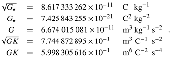
Considering the definitions $K=1/\left(4\pi {\epsilon }_0\right)$ and $G_{★}=\left(4\pi {\epsilon }_0\right)G=G/K$, the G-M constant of the cross-forces takes the following equivalent forms:

$$\sqrt{GK}=\sqrt{{\left(4\pi {\epsilon }_0\right)}^{-1}G}=K\sqrt{G_{★}}={\displaystyle \frac{\sqrt{G_{★}}}{4\pi {\epsilon }_0}},$$

(13)

and its SI value is, to 10 significant digits,

$$\sqrt{GK}=7.744872895\times {10}^{-1}{\mathrm{m}}^3{\mathrm{C}}^{-1}{\mathrm{s}}^{-2},$$

(14)

where we have used the recently determined value [3] of Newton’s G, viz.

$$G=6.674015081\times {10}^{-11}{\mathrm{m}}^3{\mathrm{kg}}^{-1}{\mathrm{s}}^{-2}.$$

(15)

2.4. The Sources of the Cross-Field

The last expression of the G-M constant in equation (13) can be used to cast the conservative cross-forces in ‘standard vector form’ [3], viz.

$$\left(\begin{array}{c}{F}_{M\to q}\\ F_{Q\to m}\end{array}\right)={\displaystyle \frac{\sqrt{G_{★}}}{4\pi {\epsilon }_0{r}^2}}\left(\begin{array}{c}Mq\\ Qm\end{array}\right).$$

(16)

Then, Gauss’s law provides the cross-field fluxes ${\mathcal{F}}_{\times }$ that can be written in vector form as

$$\left(\begin{array}{c}{\mathcal{F}}_{\times M}\\ {\mathcal{F}}_{\times Q}\end{array}\right)={\displaystyle \frac{\sqrt{G_{★}}}{{\epsilon }_0}}\left(\begin{array}{c}M\\ Q\end{array}\right).$$

(17)

Equation (17) shows that the same G-M constant couples to masses and charges to generate the sources of the cross-fields, viz. $\left(\sqrt{G_{★}}M\right)$ and $\left(\sqrt{G_{★}}Q\right)$, according to Gauss’s law (in classical literature, the presence of ${\epsilon }_0$ is neglected in descriptions of source terms). These sources should be contrasted to the well-known sources $\left(G_{★}M\right)$ of gravitational field and $\left(Q\right)$ of the electric field (as shown in the flux equations (11) and (12) of Ref. [3]). In all equations, the introduction of the effective gravitational constant $G_{★}$ (in place of Newton’s G) is necessary to ensure the appearance of ${\epsilon }_0^{-1}$ (the factor that is not discussed in descriptions of source terms) in all four forms of Gauss’s law.

3. Constants of Nature Produced by G-M Averaging of Known Constants

Our exploration of G-Ms as they appear in various physical contexts started with MOND theory and varying-G gravity [1] and with atomic and particle physics [2]; and it was recently expanded to properties of conservative fields influenced by (geometric and physical) constraints imposed by the vacuum [3]. In Section 1 and Section 2 above, we elaborated on some well-known and some new physical constants that evidently have an important meaning in natural processes, and that deserve a more detailed investigation, because they reveal the intrinsic couplings present in the various forces observed in nature.

We analyze below the constants generated by the G-Ms of G and $4\pi {\epsilon }_0$ and by the G-Ms of $G_{★}$ and $e^2$ (Section 1.3(c)), and we also include the weak coupling constant

$${\mathsf{\alpha }}_{\mathrm{w}}=\sqrt{\mathsf{\alpha }},$$

(18)

introduced in Section 1.3(c) (item ②) above. In this case, ${\mathsf{\alpha }}_{\mathrm{w}}$ appears to be the G-M of the constituent terms that make up the fine-structure constant $\mathsf{\alpha }$.

3.1. The Geometric Means of  G and $4\pi {\epsilon }_0$

From G and $4\pi {\epsilon }_0=1/K$, two G-Ms can be formed, viz.

$$\sqrt{G_{★}}=\sqrt{4\pi {\epsilon }_0·G}\mathrm{and}\sqrt{H_{★}}=\sqrt{G·K}.$$

(19)

Their numerical values are given to a precision of 10 significant digits in Section 1.3(c) (item ⑥) and equation (14), respectively. Furthermore, $\mathcal{N}\left(\sqrt{G_{★}}\right)=\mathcal{N}\left(k_{\mathrm{B}}\right)$ when Boltzmann’s constant $k_{\mathrm{B}}$ is expressed in MeV ${\mathrm{K}}^{-1}$, from which we have determined the value of Newton’s G shown in equation (15).

Both G-Ms attest to an interplay between gravity and the vacuum in which gravity is constrained in two different ways: Since vacuum permittivity ${\epsilon }_0$ is a lower limit, then $G_{★}$ attains a minimum value in the gravitational interactions $M\rightleftharpoons m$ (equation (8) written in terms of $G_{★}$ in our ‘standard form’ [3]), whereas $\sqrt{H_{★}}\propto {\epsilon }_0^{-1/2}$ attains a maximum value in the cross-forces $M\rightleftharpoons q$ and $Q\rightleftharpoons m$ (equations (11) and (12)).

This comparison leads to an important conclusion: evidently, the vacuum restricts the strength of the gravitational forces much more than the strength of the cross-conservative forces. The ratio of the two G-M values is $\mathcal{N}(\sqrt{H_{★}}/\sqrt{G_{★}})=\mathcal{N}\left(K\right)\sim {10}^{10}$. We have advocated the same conclusion in Ref. [3] (see Equation (14) in that paper).

3.2. The Geometric Means of  $G_{★}$ and $e^2$

From $G_{★}$ and $e^2$, two G-Ms can be formed, viz.

$$L_{★}=\sqrt{e^2·G_{★}}\mathrm{and}{M}_{★}=\sqrt{e^2·G_{★}^{-1}},$$

(20)

where $L_{★}=1.380649\times {10}^{-29}$ ${\mathrm{C}}^2$ ${\mathrm{kg}}^{-1}$ and $M_{★}=1.859249\times {10}^{-9}$ kg.

The numerical value of $L_{★}$ is encountered in thermodynamics, viz.

$$\mathcal{N}\left(L_{★}\right)=\mathcal{N}\left(k_{\mathrm{B}}\right)\times {10}^{-6}$$

(21)

(see also in Section 1.3(c), items ⑥ and ⑦). On the other hand, the G-M $M_{★}$ is a new universal constant with dimensions of [mass] and a Planck-scale magnitude.

We analyze each of these constants below.

3.2.1. The G-M Constant $M_{★}$

Physical interpretation.—The new constant mass $M_{★}$ admits two concordant interpretations:

(a)

The attractive Newtonian force between two $M_{★}$ masses separated by distance r has the same magnitude as the repulsive Coulomb force between two electrons or protons at the same distance r, viz.

$${\displaystyle \frac{G{M}_{★}^2}{r^2}}={\displaystyle \frac{K{e}^2}{r^2}}\Rightarrow {\displaystyle \frac{G_{★}{M}_{★}^2}{r^2}}={\displaystyle \frac{e^2}{r^2}}.$$

(22)

(b)

The repulsive cross-force of mass $M_{★}$ on to an electron at distance r (or the attractive reaction force on to $M_{★}$) has the same magnitude as the repulsive Coulomb force between two electrons or protons at distance r, viz.

$${\displaystyle \frac{\left(\sqrt{H_{★}}{M}_{★}\right)e}{r^2}}={\displaystyle \frac{K{e}^2}{r^2}}\mathrm{or}{\displaystyle \frac{\left(\sqrt{GK}{M}_{★}\right)e}{r^2}}={\displaystyle \frac{K{e}^2}{r^2}}.$$

(23)

The cross-force $M_{★}\to e$ repels the electron that brings a negative sign to the interaction. On the other hand, the reaction force $e\to M_{★}$ attracts the mass because the Coulomb cross-field $e<0$ operates on to the oppositely-signed $M_{★}>0$. Along the same line of reasoning, the cross-force $M_{★}\to p$ attracts a proton p, and the reaction force $p\to M_{★}$ repels $M_{★}$. Thus, the cross-fields do not only exhibit an entirely new coupling constant (the G-M $\sqrt{GK}$), but they also operate in different directions in 3D space compared to the conventional gravitational and electrostatic fields.

Relationship to the Planck mass.—The new constant mass $M_{★}$ is related to the Planck mass $M_{\mathrm{P}}$ in a fundamental way. We define $M_{\mathrm{P}}$ in terms of Planck’s h (not in terms of ℏ [2,3]), viz.

$$M_{\mathrm{P}}\equiv \sqrt{{\displaystyle \frac{hc}{G}}}=5.45562831\times {10}^{-8}\mathrm{kg},$$

(24)

and we find precisely that

$$M_{★}=M_{\mathrm{P}}\sqrt{\mathsf{\alpha }}=M_{\mathrm{P}}{\mathsf{\alpha }}_{\mathrm{w}},$$

(25)

according to the world average value of $\mathsf{\alpha }$ given by the Particle Data Group (PDG) [31,32,33].

The two lower scalings of the Planck mass.—It is interesting to note that, in conjunction to the recent results presented in Ref. [2], the Planck mass is scaled down to two different mass scales by different ‘squared-rooted’ (i.e., G-M) universal constants:

(a)

First, $M_{\mathrm{P}}$ is scaled down to the much smaller (subatomic) mass $M_{\mathrm{A}}=15.0$ MeV/$c^2$ [2] by the dimensionless constant $\sqrt{{\mathsf{\beta }}_{\mathrm{g}}}=4.899496947\times {10}^{-22}$, where the normalized gravitational constant ${\mathsf{\beta }}_{\mathrm{g}}$ [3] is given by

$${\mathsf{\beta }}_{\mathrm{g}}\equiv G_{★}{\left({\displaystyle \frac{m_{\mathrm{e}}}{e}}\right)}^2=2.400507034\times {10}^{-43},$$

(26)

and it represents the ratio $E_{\mathrm{grav}}/E_{\mathrm{elec}}$ of the gravitational to the electrostatic energy between two electrons separated by any distance r. The numerical value of ${\mathsf{\beta }}_{\mathrm{g}}$ was obtained from the new value of Newton’s G (equation (15)) and the CODATA values of e and $m_{\mathrm{e}}$ [6], and it is precise to 10 significant digits.

(b)

Second, equation (25) indicates that $M_{\mathrm{P}}$ is also scaled down to $M_{★}$ by $\sqrt{\mathsf{\alpha }}$. Mass $M_{★}$ was first obtained in Ref. [2] from an altogether different perspective, and it was expressed in atomic units (GeV/$c^2$). The argument was that, if the gravitational coupling constant ${\mathsf{\alpha }}_{\mathrm{g}}\equiv G{m}_{\mathrm{e}}^2/\left(hc\right)$ is running at higher energies, then ${\mathsf{\alpha }}_{\mathrm{g}}$ meets the fine-structure constant $\mathsf{\alpha }$ (i.e., ${\mathsf{\beta }}_{\mathrm{g}}=1$) at the critical mass $M_{★}=1.042962\times {10}^{18}$ GeV/$c^2$. Thus, the critical mass $M_{★}$ may also be determined from equation (26) by letting ${\mathsf{\beta }}_{\mathrm{g}}\to 1$ and $m_{\mathrm{e}}\to M_{★}$.

3.2.2. The G-M Constant $L_{★}$

Physical interpretation.—The constant $L_{★}$ with the unusual dimensions of ${\left[Q\right]}^2·{\left[M\right]}^{-1}$ is not new. It appears prominently in the Reissner-Nordström metric [34,35] which, in addition to the Schwarzschild radius $R_S=2GM/c^2$ of a nonrotating black hole, exhibits a charge radius of the form $R_Q\equiv \sqrt{Q^{2}G/\left(4\pi {\epsilon }_0{c}^4\right)}$ determined by the total charge Q of the black hole.

We write the definition of $R_Q$ for the elementary charge ($Q=e$ and $R_Q\to R_e$), and we cast its equation in a form that is much easier to interpret in the context of a charged nonrotating black hole, viz.

$$R_e\equiv \sqrt{{\displaystyle \frac{e^{2}G}{4\pi {\epsilon }_0{c}^4}}}={\displaystyle \frac{{\mu }_0}{4\pi }}\sqrt{e^2{G}_{★}}={\displaystyle \frac{{\mu }_0}{4\pi }}{L}_{★}=1.380649\times {10}^{-36}\mathrm{m}.$$

(27)

We see now that $R_e$ is the G-M of $e^2$ and $G_{★}$ (or $L_{★}$) suitably scaled by ${\mu }_0/\left(4\pi \right)$, which readily provides the correct units and a precise coefficient of ${10}^{-7}$ [6]. (This is indeed the nature of ${\mu }_0/\left(4\pi \right)$, to always carry the 3D $\left(4\pi \right)$ imprint with it, and to always provide a scaling coefficient of ${10}^{-7}$.)

Relationships to Boltzmann’s constant and the Planck length.— Because of the appearance of $L_{★}$ in equations (21) and (27), the above numerical value of $R_e$ turns out to be related to the SI value of Boltzmann’s constant $k_{\mathrm{B}}$, viz.

$$\mathcal{N}\left(R_e\right)=\mathcal{N}\left(k_{\mathrm{B}}\right)\times {10}^{-13}.$$

(28)

Furthermore, the length scale provided by $R_e$ is related to the Planck length $L_{\mathrm{P}}$ in a fundamental way. We define $L_{\mathrm{P}}$ in terms of Planck’s h (not in terms of ℏ [2,3]), viz.

$$L_{\mathrm{P}}\equiv \sqrt{{\displaystyle \frac{hG}{c^3}}}=4.05126407\times {10}^{-35}\mathrm{m},$$

(29)

and we find precisely that

$$R_e=L_{\mathrm{P}}\sqrt{\mathsf{\alpha }}=L_{\mathrm{P}}{\mathsf{\alpha }}_{\mathrm{w}},$$

(30)

according to the world average value of $\mathsf{\alpha }$ given by the PDG [31,32,33].

Finally, we multiply equations (25) and (30), and we find a new relation between $\mathsf{\alpha }$, the Compton length $r_{\mathrm{c}}$, and the new G-Ms, viz.

$$\mathsf{\alpha }=\left({\displaystyle \frac{M_{★}}{m_{\mathrm{e}}}}\right)\left({\displaystyle \frac{R_e}{r_{\mathrm{c}}}}\right)={\displaystyle \frac{{\mu }_0}{4\pi }}\left({\displaystyle \frac{M_{★}}{m_{\mathrm{e}}}}\right)\left({\displaystyle \frac{L_{★}}{r_{\mathrm{c}}}}\right),$$

(31)

where $m_{\mathrm{e}}$ is the electron mass and the G-Ms are given by equation (20).

Physical numerology.—Equations (21) and (28) demonstrate two precise numerical relations between physical constants that carry different units. Although the numerical equalities are precise (they agree to 7-10 significant digits), they cannot be categorized to either one of the two classes of numerological formulae specified by I. J. Good [36]. In 1990, Good wrote:

• “When a numerological formula is proposed, then we may ask whether it is correct. The notion of exact correctness has a clear meaning when the formula is purely mathematical, but otherwise some clarification is required. I think an appropriate definition of correctness is that the formula has a good explanation, in a Platonic sense, that is, the explanation could be based on a good theory that is not yet known but ‘exists’ in the universe of possible reasonable ideas.”

Equations (21) and (28) belong to a new class of numerological formulae that are certainly not approximate, yet they do require a physical explanation according to Good’s ideas [36]. Our explanation is that nature applies its restrictions (or thresholds) with the same strength in different physical contexts; she would not be able to do otherwise, if she is deterministic in the macrocosm. Therefore, the numerical coincidences between various (seemingly unrelated) natural constants reveal nature’s capability across the entire spectrum of phenomena, those phenomena that we, researchers, have treated and analyzed separately in the general realm of the physical sciences.

This is an important assertion: We believe that force unification would not be possible without accounting for this much wider context across fields of the physical sciences. It also signifies that writing down ad-hoc Lagrangians that use many different coupling constants to introduce various subatomic interactions between particles (e.g., Ref. [37]) will not succeed in producing the comprehensive Lagrangian of the unified field because the many ad-hoc constants are numerically related [2,3], most of them by G-Ms. Some such relations are described in the remainder of the paper.

Additional precise numerical concurrences.—By combining equations (28) and (30), we establish the unusual numerical equality

$$\mathcal{N}\left(k_{\mathrm{B}}\right)=\left({10}^{13}{\mathsf{\alpha }}_{\mathrm{w}}\right)\mathcal{N}\left(L_{\mathrm{P}}\right).$$

(32)

Next, by introducing the Planck temperature $T_{\mathrm{P}}=M_{\mathrm{P}}{c}^2/k_{\mathrm{B}}=3.551427\times {10}^{32}$ K in place of $k_{\mathrm{B}}$ in equation (32), we derive a numerical expression for the weak coupling constant ${\mathsf{\alpha }}_{\mathrm{w}}$ in terms of (h-defined) Planck scales, viz.

$${\mathsf{\alpha }}_{\mathrm{w}}=\left[{\displaystyle \frac{\mathcal{N}\left(F_{\mathrm{P}}\right)}{\mathcal{N}\left(T_{\mathrm{P}}\right)}}\right]\times {10}^{-13},$$

(33)

where $F_{\mathrm{P}}=c^4/G=1.21030723\times {10}^{44}$ N is the Planck force.

Thus, the weak coupling constant ${\mathsf{\alpha }}_{\mathrm{w}}$, and by extension the fine-structure constant $\mathsf{\alpha }$ (since ${\mathsf{\alpha }}_{\mathrm{w}}=\sqrt{\mathsf{\alpha }}$), the two fundamental constants of atomic physics are clearly related to the numerical values of the Planck constants $F_{\mathrm{P}}$ and $T_{\mathrm{P}}$. Equation (33) demonstrates a previously unknown relationship between the magnitudes of atomic and cosmological constants, and it also justifies our arguments against using the 2D constant $\hslash =h/\left(2\pi \right)$ in the definitions of intrinsically 3D physical quantities, such as $\mathsf{\alpha }$ and ${\mathsf{\alpha }}_{\mathrm{w}}$ [2,3].

We note however that equations in which $\hslash /2$ (i.e., $h/\left(4\pi \right)$, where $4\pi$ signifies 3D geometry) is inserted (e.g., Heisenberg’s uncertainty principle [38] or the quantized angular momentum of the ring singularity in the Kerr-Newman metric [39]) are still correct and valid, as they are applicable to 3D space. Unfortunately, this is not the case in the traditional definition of the fine-structure constant, which (we insist) should be defined as in equation (3) above. After all, only then does the fundamental relation (18) become apparent, and an important connection between electrodynamics and particle physics emerges from the shadow of ℏ.

3.3. The G-M That Produces the Weak Coupling Constant ${\mathsf{\alpha }}_{\mathrm{w}}$ and the Second G-M

3.3.1. The Weak Coupling Constant as a G-M

Although not immediately apparent, equation (18) represents yet another G-M that produces the weak coupling constant ${\mathsf{\alpha }}_{\mathrm{w}}$. The G-M of ${\mathsf{\alpha }}_{\mathrm{w}}$ becomes evident when we replace the fine-structure constant from its definition (3), viz.

$${\mathsf{\alpha }}_{\mathrm{w}}=\sqrt{e^2·{\displaystyle \frac{1}{4\pi {\epsilon }_{0}hc}}}.$$

(34)

The square-rooted denominator represents the Planck charge $Q_{\mathrm{P}}$ [40], albeit expressed in terms of Planck’s h, so we define

$$Q_{\mathrm{P}}\equiv \sqrt{4\pi {\epsilon }_{0}hc}=4.70129673\times {10}^{-18}\mathrm{C},$$

(35)

and we rewrite equation (34) as

$${\mathsf{\alpha }}_{\mathrm{w}}=\sqrt{e^2·{Q_{\mathrm{P}}}^{-2}}={\displaystyle \frac{e}{Q_{\mathrm{P}}}}=0.034079462.$$

(36)

This is another unexpected relation between the weak coupling constant and the Planck charge. An analogous equation has been previously obtained for the fine-structure constant (see Equation (44) in Ref. [2]).

3.3.2. The Second G-M and Associated Planck Units

The second G-M of that shown in equation (34), viz.

$$Q_{★}^2\equiv \sqrt{e^2·4\pi {\epsilon }_{0}hc}=e{Q}_{\mathrm{P}},$$

(37)

is unusual because it has dimensions of [charge]². Thus, $Q_{★}$ represents yet another charge scale in addition to the well-known charges e and $Q_{\mathrm{P}}$ (equation (35)), and it is in fact the G-M of e and $Q_{\mathrm{P}}$. We explore its significance below.

We multiply and divide by Newton’s G under the square root in equation (37), and we obtain the relations

$$Q_{★}^2\equiv \sqrt{(e^2·G_{★}){\displaystyle \frac{hc}{G}}}=M_{\mathrm{P}}\sqrt{e^2·G_{★}}=M_{\mathrm{P}}{L}_{★},$$

(38)

where $M_{\mathrm{P}}$ and $L_{★}$ are given by equations (24) and (20), respectively. Thus, $Q_{★}$ is also the G-M of $M_{\mathrm{P}}$ and $L_{★}$.

The new charge $Q_{★}=8.678887\times {10}^{-19}$ C includes contributions from electromagnetism (e), gravity (G), the vacuum ($4\pi {\epsilon }_0$), and the Planck units ($M_{\mathrm{P}}$). From the point of view of the vacuum, $Q_{★}$ represents a minimum value, since ${\epsilon }_0$ is a lower limit in nature. By comparison, the Planck charge (35) is also limited by the vacuum, viz.

$$Q_{\mathrm{P}}=M_{\mathrm{P}}\sqrt{G_{★}},$$

(39)

where $4\pi {\epsilon }_0$ is embedded in the definition of $G_{★}$; but $Q_{\mathrm{P}}$ does not depend on the elementary charge e.

In contrast, e, the smallest of the three charges, is the only charge which is amplified by the vacuum (the factor of $4\pi {\epsilon }_0$ divides e in the electrostatic source term that appears in Coulomb’s law and Gauss’s law). Examining the relative strengths of these charges, we determine a universal dimensionless ratio, the common ratio $r_Q$ of the geometric progression of the charges, viz.

$$r_Q\equiv {\displaystyle \frac{Q_{\mathrm{P}}}{Q_{★}}}={\displaystyle \frac{Q_{★}}{e}}=5.416935={{\mathsf{\alpha }}_{\mathrm{w}}}^{-1/2},$$

(40)

with a reciprocal ratio of ${r_Q}^{-1}=0.1846062=\sqrt{{\mathsf{\alpha }}_{\mathrm{w}}}$ (see also the ratio $e/Q_{\mathrm{P}}={\mathsf{\alpha }}_{\mathrm{w}}={r_Q}^{-2}$ shown in equation (36)).

3.3.3. Distinguished Electromagnetic Planck Units

Finally, we return to equation (39) that describes the Planck charge effectively as the G-M $\sqrt{M_{\mathrm{P}}^2·G_{★}}$. This G-M reminds us of $L_{★}$, the G-M of $e^2$ and $G_{★}$ (see equation (20)). The analogy between G-Ms continues in the original (h-defined) Planck system when we determine the uncommon units of capacitance $C_{\mathrm{P}}$ and magnetic flux ${\mathsf{\Phi }}_{\mathrm{P}}$:

(a)

The unit of capacitance is $C_{\mathrm{P}}=\left(c^{-2}\right)\sqrt{Q_{\mathrm{P}}^2·G_{★}}$, where $c^{-2}$ is a scaling coefficient of the G-M. Substituting $Q_{\mathrm{P}}$ from equation (39), we find for the Planck capacitance the equivalent relation

$$C_{\mathrm{P}}={\displaystyle \frac{G_{★}{M}_{\mathrm{P}}}{c^2}}.$$

(41)

This relation should be compared to the Schwarzschild-like equation $L_{\mathrm{P}}=G{M}_{\mathrm{P}}/c^2$ in the Planck system of units, and these two equations also imply that $C_{\mathrm{P}}=4\pi {\epsilon }_0{L}_{\mathrm{P}}$.

(b)

The unit of magnetic flux is ${\mathsf{\Phi }}_{\mathrm{P}}={\left(4\pi {\epsilon }_{0}c\right)}^{-1}\sqrt{M_{\mathrm{P}}^2·G_{★}}={\left(4\pi {\epsilon }_{0}c\right)}^{-1}{Q}_{\mathrm{P}}$, where ${\left(4\pi {\epsilon }_{0}c\right)}^{-1}$ is a scaling coefficient of the G-M, which also represents the Planck unit of electric resistance ${\mathcal{R}}_{\mathrm{P}}$. We have previously identified ${\mathcal{R}}_{\mathrm{P}}$ with the impedance of free space properly imprinted by the 3D geometric term of $4\pi$, viz. ${\mathcal{R}}_{\mathrm{P}}\equiv Z_0/\left(4\pi \right)$ [3]. Thus, the unit of magnetic flux can cast in the simple form

$${\mathsf{\Phi }}_{\mathrm{P}}={\mathcal{R}}_{\mathrm{P}}{Q}_{\mathrm{P}}.$$

(42)

Substituting $Q_{\mathrm{P}}$ from equation (39), we also find that ${\mathsf{\Phi }}_{\mathrm{P}}={\mathcal{R}}_{\mathrm{P}}{M}_{\mathrm{P}}\sqrt{G_{★}}$. This particular relation, as well as equation (41), shows the blending of gravity (G and $M_{\mathrm{P}}$) with vacuum constants (${\epsilon }_0$ and c) in generating profound electromagnetic constants and units. We presume that, were it not for the supporting information provided above, this statement would have been taken with a grain of salt because, in the conventional Planck system, the units $Q_{\mathrm{P}}$, ${\mathcal{R}}_{\mathrm{P}}$, and ${\mathsf{\Phi }}_{\mathrm{P}}$ apparently do not depend on Newton’s G, and the factor $G/c^4$ (and G) in the unit of capacitance $C_{\mathrm{P}}$ can be essentially eliminated in favor of the unit of force $F_{\mathrm{P}}=c^4/G$ [2,40,41].

4. Conclusions

We summarize our conclusions from this investigation as follows:

(1)

An investigation of cross-forces in a combined gravitational and electrostatic field yields physically understood results. The new coupling constant that also balances the units in the equations of these cross-forces is the G-M $\sqrt{GK}$ of the known constants G (Newton’s constant) and K (Coulomb’s constant). Thus, there is no need to introduce yet another independent constant to describe cross-interactions between masses and charges and vice versa (Section 2).

(2)

G-M averaging is pervasive in nature and in physics. Nature uses G-Ms in abundance to generate new universal constants, and physicists have used G-Ms (heretofore unknowingly) to define many (if not all) physical variables conveniently used in our explorations of the contents of the universe (Section 1 and Section 3).

(3)

By delineating nature’s G-Ms, we get a bird’s eye view at her mathematical prowess [1,2,3,9]. More than that, we have discovered that nature uses the same numerical values (‘strengths’) in what we perceive as disjoint physical contexts (Section 3 and Ref. [3]). In retrospect, how could nature have possibly done otherwise? Different numbers exist to describe differing strengths of various agents (and physical thresholds), but each agent should consistently exert the same level of strength across different settings in the same system of units and measurements. In this respect, the SI system of units is self-consistent (unlike the cgs system), as it does not reset the values of various physical constants for the sake of convenience.

(4)

Application of the same numerical value in different settings has led us to derive the following equivalent strengths of universal constants irrespective of their units in the metric (SI) system: MOND critical acceleration $a_0$ with $\mathcal{N}\left(a_0\right)=\mathcal{N}\left(4\pi {\epsilon }_0\right)$; MOND universal constant ${\mathcal{A}}_0$ with $\mathcal{N}\left({\mathcal{A}}_0\right)=\mathcal{N}\left(G_{★}\right)$; effective gravitational constant $G_{★}$ with $\mathcal{N}\left(\sqrt{e^2{G}_{★}}\right)=\mathcal{N}\left(k_{\mathrm{B}}\right)\times {10}^{-6}$. Furthermore, several physically important G-Ms of natural constants were found to be related to Planck units (Section 3.2 and Section 3.3).

(5)

The above numerical equivalence of $\sqrt{e^2{G}_{★}}$ to a submultiple of $k_{\mathrm{B}}$ allows for the determination of several fundamental constants to an unprecedented precision of 10 significant digits:

(43)

(6)

We have shown that using ℏ in physics begs for insurmountable trouble. The composite constant that presently is $\hslash =h/\left(2\pi \right)$ carries an imprint of 2D geometry ($2\pi$), which is inappropriate in 3D settings and damages all man-made definitions that use ℏ in various physical settings (e.g., the fine-structure constant and the gravitational coupling constant, but not their very useful ratio ${\mathsf{\beta }}_{\mathrm{g}}={\mathsf{\alpha }}_{\mathrm{g}}/\mathsf{\alpha }$ (equation (26)) in which ℏ fortuitously cancels out). Thus, the important relations concerning G-Ms that we have described in this work do not present themselves in the contemporary equations of physics written in terms of ℏ.

(7)

Some equations in which $\hslash /2$ appears have previously issued a fair warning that no-one noticed. In this context where the 3D constant $h/\left(4\pi \right)$ appears self-consistently, we mentioned the examples of Heisenberg’s uncertainty principle and the ring singularity in the Kerr-Newman metric (see bottom of Section 3.2.2).

(8)

Reverting back to Planck’s h yields immediately spectacular results: the electroweak theory needs only one fundamental constant, the fine-structure constant $\mathsf{\alpha }$, since the weak coupling constant ${\mathsf{\alpha }}_{\mathrm{w}}$ is simply equal to $\sqrt{\mathsf{\alpha }}$ (see top of Section 3). Experimenters who measure these constants individually by various methods should take notice.

References

- Christodoulou, D. M., & Kazanas, D. 2023, Varying-G gravity. Mon. Not. R. Astron. Soc., 519, 1277.
- Christodoulou, D. M., & Kazanas, D. 2023, The upgraded Planck system of units that reaches from the known Planck scale all the way down to subatomic scales. Astronomy, 2, 235. [CrossRef]
- Christodoulou, D. M., & Kazanas, D. 2025, Introducing the effective gravitational constant 4πε0G. Axioms, 00, 00.
- Lie, S. 1881, On integration of a class of linear partial differential equations by means of definite integrals. Archiv. Math. Nat., 6, 328.
- Abramowitz, M., & Stegun, I. A. Handbook of Mathematical Functions with Formulas, Graphs, and Mathematical Tables. Dover: New York, NY, USA, 1972, p. 10, item 3.1.6.
- Tiesinga, E., Mohr, P. J., Newell, D. B., & Taylor, B. N. 2021, CODATA recommended values of the fundamental physical constants: 2018. Rev. Mod. Phys., 93, 025010. [CrossRef]
- Planck, M. 1899, About irreversible radiation processes. Sitzungsberichte Der Preuss. Akad. Wiss., 440.
- Planck, M. 1900, Ueber irreversible Strahlungsvorgänge. Ann. Phys., 4, S.69.
- Christodoulou, D. M., O’Leary, J., Melatos, A., Kimpson, T., Bhattacharya, S., Laycock, S. G. T. O’Neill, N. J., Meyers, P. M., & Kazanas, D. 2025, Magellanic accretion-powered pulsars studied via an unscented Kalman filter. Astrophys. J., 00, 00.
- Melatos, A., O’Neill, N. J., Meyers, P. M., & O’Leary, J. 2023, Tracking hidden magnetospheric fluctuations in accretion-powered pulsars with a Kalman filter. Astrophys. J., 944, 64. [CrossRef]
- O’Leary, J., Melatos, A., O’Neill, N. J., et al. 2024, Measuring the magnetic dipole moment and magnetospheric fluctuations of SXP 18.3 with a Kalman filter. Astrophys. J., 965, 102. [CrossRef]
- O’Leary, J., Melatos, A., Kimpson, T., et al. 2024, Measuring the magnetic dipole moment and magnetospheric fluctuations of accretion-powered pulsars in the Small Magellanic Cloud with an unscented Kalman filter. Astrophys. J., 971, 126. [CrossRef]
- O’Leary, J., Melatos, A., Kimpson, T., et al. 2025, Observing Rayleigh-Taylor stable and unstable accretion through a Kalman filter analysis of X-ray pulsars in the Small Magellanic Cloud. Astrophys. J., 981, 150. [CrossRef]
- Einstein, A. 1907, Über das Relativitätsprinzip und die aus demselben gezogenen folgerungen. Jahrbuch der Radioaktivität und Elektronik, 4, 411.
- Einstein, A. 1925, Einheitliche Feldtheorie von Gravitation und Elektrizität. Sitzungsberichte der Preussischen Akademie der Wissenschaften, Vol. 1, 414.
- Paulson, S., Gleiser, M., Freese, K., & Tegmark, M. 2015, The unification of physics: the quest for a theory of everything. Ann. NY Acad. Sci., 1361, 18. [CrossRef]
- Misner, C. W., Thorne, K. S., & Wheeler, J. A. Gravitation. W. H. Freeman & Company: San Francisco, CA, USA, 1973.
- Mannheim, P. D., & Kazanas, D. 1991, Solutions to the Reissner-Nordström, Kerr, and Kerr-Newman problems in fourth-order conformal Weyl gravity. Phys. Rev. D, 44, 417. [CrossRef]
- Bakopoulos, A., & Kanti, P. 2014, From GEM to electromagnetism. Gen. Relativ. Grav., 46, 1742. [CrossRef]
- Balanis, C. A. Antenna theory. John Wiley & Sons: Hoboken, NJ, USA, 2005.
- Dirac, P. A. M. 1926, On the theory of quantum mechanics. Proc. R. Soc. Lond. A, 112, 661.
- Dirac, P. A. M. 1928, The quantum theory of the electron. Proc. R. Soc. Lond. A, 117, 610.
- Milgrom, M. 1983a, A modification of the Newtonian dynamics as a possible alternative to the hidden mass hypothesis. Astrophys. J., 270, 365. [CrossRef]
- Milgrom, M. 1983b, A modification of the Newtonian dynamics – Implications for galaxies. Astrophys. J., 270, 371.
- Milgrom, M. 1983c, A modification of the Newtonian dynamics: Implications for galaxy systems. Astrophys. J., 270, 384.
- Famaey, B., & McGaugh, S. S. 2012, Modified Newtonian Dynamics (MOND): Observational phenomenology and relativistic extensions. Living Rev. Rel., 15, 10. [CrossRef]
- Milgrom, M. 2014, MOND laws of galactic dynamics. Mon. Not. R. Astron. Soc., 437, 2531. [CrossRef]
- Milgrom, M. 2015, MOND theory. Can. J. Phys., 93, 107.
- Boltzmann, L. Vorlesungen über gastheorie. Part 1, J. A. Barth: Leipzig, Germany, 1896.
- Planck, M. Vorlesungen über die theorie der wärmestrahlung. J. A. Barth: Leipzig, Germany, 1913.
- Zyla, P. A., et al (Particle Data Group) 2020, Review of particle physics. Prog Theor Exp Phys, 2020(8), 083C01.
- Workman, R. L., Burkert, V. D., Crede, V., et al. [Particle Data Group] 2022, Review of particle physics. Prog. Theor. Exp. Phys., 2022(8), 083C01.
- Navas, S., Amsler, C., Gutsche, T. et al. [Particle Data Group] 2024, Review of particle physics. Phys. Rev. D, 110, 030001.
- Wikipedia 2025a, Reissner-Nordström metric. URL: https://en.wikipedia.org/wiki/Reissner%E2%80%93Nordstr%C3%B6m_metric (accessed on 9 March 2025).
- Wikipedia 2025b, Black hole electron. URL: https://en.wikipedia.org/wiki/Black_hole_electron (accessed on 9 March 2025).
- Good, I. J. A quantal hypothesis for hadrons and the judging of physical numerology. In G. R. Grimmett and D. J. A. Welsh (eds.) Disorder in Physical Systems. Oxford University Press: New York, NY, USA, 1990, p. 141.
- Kazanas, D., Papadopoulos, D., & Christodoulou, D. M. 2022, Gravity beyond Einstein? Yes, but in which direction? Phil. Trans. R. Soc. A, 380, 20210367. [CrossRef]
- Wikipedia 2025c, Uncertainty principle. URL: https://en.wikipedia.org/wiki/Uncertainty_principle (accessed on 9 March 2025).
- Wikipedia 2025d, Kerr-Newman metric. URL: https://en.wikipedia.org/wiki/Kerr%E2%80%93Newman_metric (accessed on 9 March 2025).
- Elert, G. 2025, The physics hypertextbook. URL: https://physics.info/planck/ (accessed on 9 March 2025).
- Wikipedia 2025e, Planck units. URL: https://en.wikipedia.org/wiki/Planck_units (accessed on 18 March 2025).
Disclaimer/Publisher’s Note: The statements, opinions and data contained in all publications are solely those of the individual author(s) and contributor(s) and not of MDPI and/or the editor(s). MDPI and/or the editor(s) disclaim responsibility for any injury to people or property resulting from any ideas, methods, instructions or products referred to in the content. |
© 2025 by the authors. Licensee MDPI, Basel, Switzerland. This article is an open access article distributed under the terms and conditions of the Creative Commons Attribution (CC BY) license (http://creativecommons.org/licenses/by/4.0/).
Copyright: This open access article is published under a Creative Commons CC BY 4.0 license, which permit the free download, distribution, and reuse, provided that the author and preprint are cited in any reuse.