
Submitted:
18 March 2025
Posted:
19 March 2025
You are already at the latest version
Abstract
In this paper, fully convolutional data description (FCDD) approach is applied to the defect detection and its concurrent visualization for industrial products and materials. Our developed MATLAB application has already allowed users to efficiently and user-friendly design, train and test various kinds of neural network (NN) models for defect detection. Supported models have been originally designed convolutional newral network (CNN), transfer learning-based CNN, NN-based suport vector machine (SVM), convolutional auto encoder (CAE), variational auto encoder (VAE), fully convolution network (FCN) such as U-Net, and YOLO, however, FCDD has not been provided yet. This paper includes the software development of the MATLAB application extended to be able to build FCDD models. In particular, a systematic threshold determination method is proposed to get the best performance for defect detection from FCDD models. Also, through three different kinds of defect detection experiments, the usefulness and effectiveness of FCDD models in terms of defect detection and its concurrent visualization of understanding are quantitatively and qualitatively evaluated by comparing conventional transfer learning-based CNN models.
Keywords:
Fully Convolutional Data Description (FCDD)
; Defect Detection
; Concurrent Visualization of Understanding
; MATLAB
1. Introduction
Recently, image data-based deep learning models such as convolutional neural network (CNN), support vector machine (SVM), convolutional auto encoder (CAE), variable auto encoder (VAE), fully convolution network (FCN) such as U-Net and so on have been applied to defect detection for various kinds of industrial products and materials. For example, after some defect is detected in inspection process using a CNN model, gradient-weighted class activation mapping (Grad-CAM) or Occlusion Sensitivity is applied to visualization process of the defect areas where the CNN is gazing. This means that defect detection process and visualization one have to be separately employed in the production line.
In this paper, fully convolutional data description (FCDD) approach [1] is applied to the defect detection and its concurrent visualization of two kinds of industrial products and an industrial material. As for FCDD, Jang and Bae proposed an anomaly detection system which was understood through FCDD trained only using OK samples to provide related users with details such as detection results of abnormal defect patterns, defect size, and location of defect patterns on wafer bin map [2]. The effectiveness is analyzed using open dataset, providing promising results of the proposed anomaly detection system. Also, Yasuno et al. reported obtained accurate and explainable results demonstrating experimental studies on concrete damage and steel corrosion in civil engineering [3]. In addition, to develop a more robust application, they applied their method to another outdoor domain that contains complex and noisy backgrounds using natural disaster datasets collected using various devices. Moreover, they proposed a valuable solution of deeper FCDDs focusing on other powerful backbones such as VGG16, ResNet101, and Inceptionv3 to improve the performance of damage detection and to implement ablation studies on disaster datasets.
Our developed MATLAB application for building defect detection models has already allowed users to efficiently design, train and test various kinds of models such as originally designed CNN, transfer learning-based CNN, SVM, CAE, VAE, FCN, and YOLO, however, FCDD has not been supported yet [4]. This paper includes the software development of MATLAB application extended to flexibly build FCDD models [5], in which one of desirable CNN models can be easily chosen for the backbone of an FCDD model to be designed. Also, in order to be able to quantitatively apply trained FCDD models to defect detection of industrial products or materials, threshold value, which is the distance from the center of hyper sphere, is statistically determined analyzing the distribution of anomaly scores obtained with training dataset.
Through the paper, the usefulness and effectiveness of FCDD models in terms of defect detection and its concurrent visualization of understanding are quantitatively and qualitatively evaluated by comparing conventional transfer learning-based CNN models.
2. FCDD (Fully Convolutional Data Description)
2.1. Deep One-Class Classification
Liznerski et al. proposed FCDD models, in which the concept of hyper sphere classifier (HSC) [6] was employed. In this subsection, the objective function of HSC is reviewed. The objective function of HSC is designed as
where denote a collection of sample images, and n is the number of training images. are the weights of the network , in which is the number of hidden layers, c, h, and w are the channel, height, and width of the images, respectively. Also, are labels where denotes an anomaly image, and denotes a normal image. Furthermore, is the center of hypersphere, and is the pseudo-Huber loss [7] given by
which approximates for small values of a and a straight line with slope 1 for large values of a, so that interpolation from quadratic to linear penalization can be performed. Due to HSC loss, normal samples and anomalous ones are mapped near c and away from the center c, respectively. The first term of Equation (1) becomes effective when the label of a training image is negative, i.e., . This is the pseudo Huber loss based on the distance , which quantifies how far the output of the network is from the center of hyper sphere c. As can be guessed, the closer the output of the network and c are, the smaller the value of first term becomes. On the other hand, the second term becomes effective when the label of a training image is positive, i.e., . The larger is, i.e., the farther the output of the network is from c, the closer approaches to 0. Consequently, approaches to , i.e., 0. It is expected from the above validation results of the two terms that the network will be trained so that normal images without a defect are mapped near the center c, whereas anomalous images with a defect are located far from the center.
2.2. Fully Convolutional Data Description Model
Figure 1 illustrates the overall network structure of the authors’ designed FCDD model. In this subsection, the concept of FCDD [1] and its loss function in training are described in detail. In FCDD implementation, the center c corresponds to the bias term in the last layer of the networks, i.e., is included in the network, which is why c is omitted in the FCDD objective function. In Liznerski’s paper, an FCN model employed in the former part performs , by which a feature map downsized into is generated from an input image X. A heat map of defective regions can be produced based on the feature map. The pseudo-Huber loss in terms of an output matrix from the FCN part, i.e., a feature map is given by
where the calculation is done with element-wise operation, i.e., pixel-wisely to be able to form a heat map. The object function in training an FCDD model is given by
With the same solution about Equation (1), the first term has a valid value in case that the label of a training image is negative, i.e., , where L1 norm is divided by the total pixels of a feature map. The value can be considered as the average per one pixel. Therefore, when normal images are given to the network in training, the weights are adjusted so that each pixel forming a heat map can approach to 0.
On the other hand, the second term becomes effective when the label of a training image is anomaly (), and has a value close to 0 with the increase of the average loss per one pixel, so that the value of log function also approaches to 0 with the lapse of training time. It is confirmed from the above discussion that Equation (4) using Equation (3) enables both to minimize the sum of the averages of of non-defective images and to maximize those of defective images.
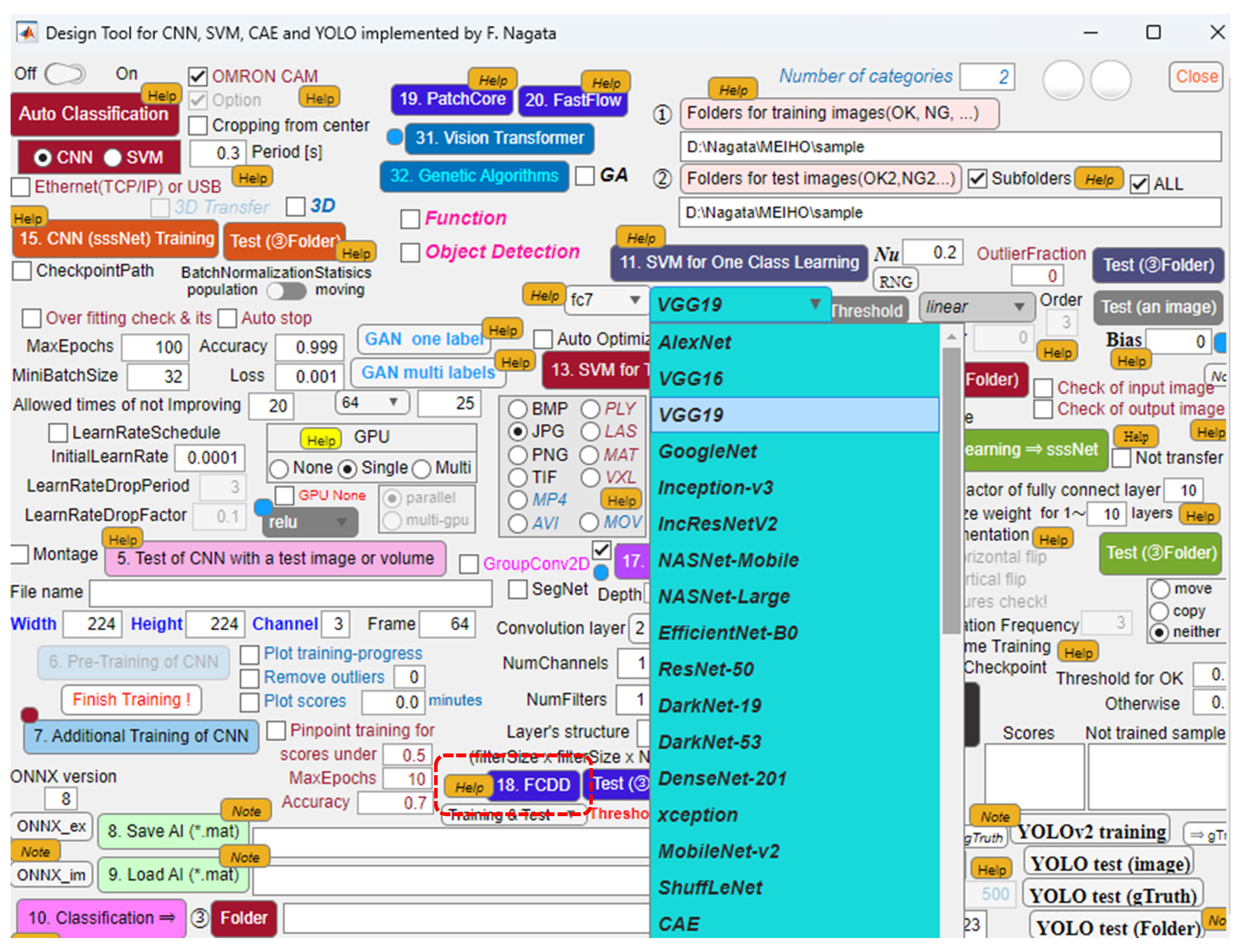
Figure 2.
Application of FCDD modeling developed on MATLAB 2024b.
2.3. How to Determine the Threshold Value for Prediction by FCDD
Figure 3 shows examples of training results. (a) is completely trained case, in which normal and anomaly samples in training dataset are completely separated. (b) is not-completely trained case, in which overlaps of normal and anomaly bins are seen. We usually face two such cases of training result according to the difficulty of given defect detection tasks. Also, it is observed from the distributions that anomaly images tend to have more variety of features than normal ones.
If a test image is given to a trained FCDD model, then the FCDD outputs a distance from the center of hypersphere. is also anomaly score given by
In order to predict whether this image is normal or abnormal, a threshold value has to be determined on horizontal axes in Figure 3(a) or Figure 3(b). In this subsection, two threshold determination methods are proposed according to (a) completely trained case and (b) not completely trained case. In the case of (a), the threshold is simply determined by
where and are the numbers of normal images and anomaly ones, and are the maximum value of and the minimum value of , respectively. On the other hand, in the case of (b), the threshold is determined by each weighted mean value including overlapped bins, which is given by
where and are the mean values of and , respectively.
Main dialogue developed on MATLAB environment as shown in Figure 2 has been extended so that FCDD models can be user-friendly trained, tested and built. The threshold value discussed in this subsection can be automatically set through this dialogue. It is expected by applying trained FCDD models to quality control process of industrial products and materials that defect detection and its clearer visualization of understanding can be concurrently conducted.
3. Comparison of Transfer Learning-Based CNN and FCDD
In this section, comparison in terms of classification accuracy and its visualization of understanding is conducted between two type of models by applying them to three kinds of tasks, i.e., two industrial products and one industrial material. The first model is well-known transfer learning-based CNN models which have been applied to various kinds of defect inspection systems in industrial fields. The second model is the authors’ interesting FCDD model introduced in the previous section. As for the dataset for training and test, casting manufacturing product images for quality inspection has been downloaded from Kaggle database [8]. Figure 4 and Figure 5 show examples of brake rotors without and with defects, respectively. In the following experiments, a VGG19-based CNN model and a VGG19-based FCDD model are evaluated and compared in terms of defect detection and its visualization.
3.1. In case of Transfer Learning-Based CNN Model Based on VGG19
The authors have applied several kinds of transfer learning-based CNN models as shown in pull down menu in Figure 2 to defect inspection of industrial products and materials [9,10]. It has been empirically confirmed from classification experiments of test images that VGG19-based transferred CNN models could always perform high accurate detection ability, so that this time also the same design approach is employed to the defect detection for comparison.
The numbers of images used are 400 OKs and 400 NGs for training dataset, and 100 OKs and 100 NGs for test dataset. After the training through 10 epochs while applying stochastic gradient decent momentum (SGDM) optimizer [11] and cross entropy loss function, the VGG19-based CNN was evaluated using the test dataset. Table 1 shows the classification result of the test dataset. As can be seen, this binary classification task of images as shown in Figure 4 and Figure 5 seems to be not difficult for the CNN model, in which only one image named `cast_def_0_571.jpeg’ shown in Figure 6 is misclassified as normal (OK). However, this false negative actually looks as a normal product since almost no defect or damage can be observed in the image. There may have been a human labeling error.
Then, visualization of understanding, i.e., where the CNN is looking at in classification, is tried to be generated using Grad-CAM [13] and Occlusion Sensitivity [14]. Figure 7 and Figure 8 show examples of visualization results. Superiority of Occlusion Sensitivity can be confirmed by comparing these two results, i.e., defect regions are identified more clearly and properly in the heat maps. Note that in this experiment, two parameters such as mask size and stride required for Occlusion Sensitivity are set to 45 and 22, respectively.
3.2. In case of FCDD
Our designed FCDD model consists of 36 layers, in which layers from 1st to 28th in original VGG19 are extracted with their powerfully-tuned weights and deployed in the encoder part of the FCDD, i.e., FCN part, for a feature extractor to produce 28×28×512 sized feature maps. In training the FCDD using the same training dataset in the previous subsection, Adam (Adaptive moment estimation) optimizer [12] is applied to tuning the weight parameters mainly for the 29th, 32nd, 35th convolution layers and 30th, 33rd batch normalization layers in the FCDD, i.e., to minimize the object function given by Equation (4). After training the FCDD model through 10 epochs, its generalization ability is simply evaluated using the same test dataset in the previous subsection, so that almost the same result is obtained as shown in Table 2. One image misclassified as false negative is checked, so that, in this case also, `cast_def_0_571.jpeg’ is confirmed. It is interesting for us that both the VGG19-based CNN and the FCDD could properly identify the `cast_def_0_571.jpeg’ as normal in spite of being labeled as anomaly in the test dataset. Actually, since `cast_def_0_571.jpeg’ looks like a normal product without defect, it can be guessed that this image is mislabeled incorrectly by human error, i.e., as a labeling noise.
Then, visualization ability for understanding the basis of classification is evaluated using the same images as shown in Figure 7 and Figure 8. In the case of the FCDD model, superior and distinct heat maps as shown in Figure 9 can be obtained without separately and additionally applying Grad-CAM or Occlusion Sensitivity.
4. Further Comparisons of CNN and FCDD
Two kinds of further comparisons similar to the experiment in the previous section are conducted to deeply evaluate the superiority of FCDD model using different datasets of a fibrous industrial material and a wrap film product.
4.1. Defect Detection and Visualization of a Fibrous Industrial Material
Figure 10 and Figure 11 show examples of fibrous industrial materials without and with defects, respectively. There are seen undesirable shape deformation defects such as frayed tip and split end.
4.1.1. In case of Transfer Learning-Based CNN Model Based on VGG19
As evaluated in the previous section, classification experiments were conducted using a VGG19-based transfer learning CNN model. The numbers of images used are 187 OKs and 214 NGs for training dataset, and 46 OKs and 55 NGs for test dataset. After training 300 epochs, we evaluated the VGG19-based CNN using the test dataset. Table 3 shows the classification result of the test dataset, in which 10 images are misclassified. The defect detection accuracy is 90.1%. Note that the original images with the large resolution of 2590×1942 have to be downsized into 224×224 as shown in Figure 12 which is that of the input layer of VGG19, so that unfortunately minute features of defects seem to be lost in some degree.
Then, two visualization tools, Grad-CAM and Occlusion Sensitivity, are applied to identify the areas where the CNN is looking at in classification. Figure 13 and Figure 14 show examples of the visualization results. Similar to the results in the previous section, the superiority of Occlusion Sensitivity is observed, however, the thin split-hair type defect is not properly identified as shown in the left side photo.
4.1.2. In case of FCDD
Similarly, after training the FCDD model for 300 epochs, its generalization ability is evaluated using the same test dataset as in the previous subsection. Table 4 shows the classification result of the test dataset. As can be seen, in the case of FCDD model also, complete defect detection was difficult due to the same cause of the decay of minute defect features as in the previous subsection. The classification accuracy is 89.1%.
4.2. Defect Detection and Visualization of a Wrap Film Product
Up to now, working and effort on systematically detecting defective wrap film products as shown in Figure 16 have been devoted by inspectors and engineers. However, there is still a problem such that sufficient detection performance cannot be obtained even if commercially available image detectors are used. The undesirable dislocation of the transparent film and the light reflection from the film seem to make the defect detection more difficult. The authors researched SVM models for the defect detection designed based on VAE model or CNN model, and tried to apply them to the detecting defective wrap film products [15].
In the 3rd test trial, wrap film products are used for comparison. Figure 16 shows non-defective and defective images on the production line, in which typical defects such as long core, deviation of rolling, protrusion of film, deformation of core, taper-shaped rolling are seen. The wrap film products are constantly fed with the same orientation through the automation line, and the snapshots of target film areas are regularly captured by a fixed camera, so that the template matching technique to crop target film area is easy to be applied [15].
A dataset for training is composed of 118 OK and 158 NG images. Also, a dataset for tesing is 468 OK and 628 NG images. All the images are in advance cropped by using the template matching method.
4.2.1. In case of Transfer Learning-Based CNN Model Based on VGG19
After training a transfer learning-based CNN model based on VGG19, the generalization ability is evaluated using the test dataset. The result is tabulated in the confusion matrix shown in Table 5, in which the detection accuracy is 98.3%. Also, Figure 17 and Figure 18 show the visualization results using Grad-CAM and Occlusion Sensitivity, respectively, when each defective image is predicted by the CNN model. As can be seen, it seems that it is not easy for these two visualizers to validly produce heat maps catching the defective areas surrounded with red dotted lines.
4.2.2. In case of FCDD
Then, after training a VGG19-based FCDD model, the generalization ability is evaluated using the same test dataset. The result is tabulated in the confusion matrix shown in Table 6, in which the detection accuracy is 98.3%. Also, Figure 19 shows the visualization results which can be concurrently produced with defect detection. As can be seen, it is observed that the FCDD model can generate more valid and clear heat maps compared to those by Grad-CAM and Occlusion Sensitivity.
5. Conclusions
Our developed MATLAB application for building defect detection models has already allowed users to efficiently design, train and test various kinds of models such as an originally designed CNN, transfer learning-based CNN, SVM, CAE, VAE, FCN, and YOLO, however, FCDD models have not been supported yet. This paper includes the software development extended to flexibly build FCDD models, by which one of desirable CNN models is easily selected for the backbone of FCDD. In this paper, VGG19-based FCDD models have been built and applied to defect detection tasks of two industrial products and one industrial material, then their detection and visualization abilities are experimentally evaluated while comparing conventional transfer learning-based CNN models with Grad-CAM and Occlusion Sensitivity. As for the generalization ability for defect detection, both models perform almost the same classification ability although, for example, the visual features of several minute defects are lost due to the downsizing of images. On the other hand, as for visualization ability of understanding, the superiorities of three FCDD models are experimentally confirmed due to its concurrent and more distinct visualization performance. One of the attractive functions of our developed FCDD designer is the flexible selection of backbone CNN to be incorporated in the former part of FCDD model. In this paper, only VGG19 is selected for the backbone due to our past empirical knowledge, however, performances of other combinations, in which other powerful CNN models such as AlexNet, GoogleNet, NASNET-Large, ResNet50, DarkNet-53 and so on are used for the backbone, have not been evaluated. In the future, therefore, FCDD models incorporated with such CNN models will be compared each other in terms of both detection accuracy and visualization of understanding.
Author Contributions
Conceptualization, F.N. and K.W.; Methodology, F.N. and S.S.; Software, F.N. and S.S.; Validation, F.N. and S.S.; Formal analysis, F.N. and S.S.; Investigation, F.N. and S.S.; Resources, F.N. and S.S.; Data curation, F.N.; Writing—original draft preparation, F.N. and M.K.H.; Writing—review and editing, F.N., M.K.H. and K.W.; Visualization, F.N. and A.S.A.G.; Supervision, F.N. All authors have read and agreed to the published version of the manuscript.
Funding
This research received no external funding.
Data Availability Statement
Data are contained within the article.
Conflicts of Interest
The authors declare no conflicts of interest.
Abbreviations
The following abbreviations are used in this manuscript:
| ADAM | Adaptive Moment Estimation Optimizer |
| CAE | Convolutional Auto Encoder |
| CNN | Convolutional Neural Network |
| FCDD | Fully Convolutional Data Description |
| FCN | Fully Convolution Network |
| Grad-CAM | Gradient-Weighted Class Activation Mapping |
| HSC | Hyper Sphere Classifier |
| SGDM | Stochastic Gradient Decent Momentum Optimizer |
| SVM | Support Vector Machine |
| VAE | Variational Auto Encoder |
References
- P. Liznerski, L. Ruff, R.A. Vandermeulen, B.J. Franks, M. Kloft, K.R. Muller, “Explainable Deep One-Class Classification," Procs. of ICLR2021, pp. 1–25, 2021. [CrossRef]
- S.J. Jang, S.J. Bae, “Detection of Defect Patterns on Wafer Bin Map Using Fully Convolutional Data Description (FCDD),” Journal of Society of Korea Industrial and Systems Engineering, Vol. 46 No. 2, pp.1–12, 2023. [CrossRef]
- T. Yasuno, M. Okano, J. Fujii, “One-class Damage Detector Using Deeper Fully Convolutional Data Descriptions for Civil Application,” Artificial Intelligence and Machine Learning, Vol. 3, No. 2, pp. 996–1011, 2023. [CrossRef]
- F. Nagata, K. Nakashima, K. Miki, K. Arima, T. Shimizu, K. Watanabe, M.K. Habib, “Design and Evaluation Support System for Convolutional Neural Network, Support Vector Machine and Convolutional Autoencoder," Measurements and Instrumentation for Machine Vision, pp. 66–82, CRC Press, Taylor & Francis Group, July, 2024.
- F. Nagata, S. Sakata, H. Kato, K. Watanabe, M.K. Habib, Defect Detection and Visualization of Understanding Using Fully Convolutional Data Description Models, Procs. of 16th IIAI International Congress on Advanced Applied Informatics, pp. 78–83, 2024.
- L. Ruff, R.A. Vandermeulen, B.J. Franks, K.R. Muller, and M. Kloft, “Rethinking assumptions in deep anomaly detection," arXiv preprint arXiv:2006.00339, 2020.
- P.J. Huber, “Robust Estimation of a Location Parameter," The Annals of Mathematical Statistics, Vol. 35, No. 1, pp. 73–101, 1964.
- Kaggle: San Francisco, CA, USA, 2020. Available online: https://www.kaggle.com/datasets/ravirajsinh45/real-life-industrial-dataset-of-casting-product?resource=download-directory (accessed on 20 March 2025).
- K. Arima, F. Nagata, T. Shimizu, A. Otuka, H. Kato, K. Watanabe, M.K. Habib, “Improvements of Detection Accuracy and Its Confidence of Defective Areas by YOLOv2 Using a Dataset Augmentation Method," Artificial Life and Robotics, Springer, Vol. 28, No. 3, pp. 625–631, 2023. [CrossRef]
- T. Shimizu, F. Nagata, K. Arima, K. Miki, H. Kato, A. Otsuka, K. Watanabe, M.K. Habib, “Enhancing Defective Region Visualization in Industrial Products Using Grad-CAM and Random Masking Data Augmentation," Artificial Life and Robotics, Springer, Vol. 29, No. 1, pp. 62–69, 2023. [CrossRef]
- K.P., Murphy, “Machine Learning: A Probabilistic Perspective," The MIT Press, Cambridge, Massachusetts, 2012.
- D. Kingma, J. Ba, “Adam: A Method for Stochastic Optimization." Procs. of the 3rd International Conference on Learning Representations (ICLR 2015), 15 pages, 2015.https://arxiv.org/pdf/1412.6980.pdf (accessed on 15 February 2024).
- R.R. Selvaraju, M. Cogswell, A. Das, R. Vedantam, D. Parikh, D. Batra, “Grad-CAM: Visual Explanations from Deep Networks via Gradient-based Localization," Procs. of IEEE International Conference on Computer Vision (ICCV), pp. 618–626, 2017.
- M.D. Zeiler, R. Fergus, Computer Vision – ECCV 2014: 13th European Conference, Proceedings, Part III (Lecture Notes in Computer Science, 8691), pp. 818–833, Springer, 2014.
- T. Shimizu, F. Nagata, M.K. Habib, K. Armina, A. Otsuka, K. Watanabe, Advanced Defect Detection in Wrap Film Products: A Hybrid Approach with Convolutional Neural Networks and One-Class Support Vector Machines with Variational Autoencoder-Derived Covariance Vectors, Machines, Vol. 12, No. 9, pp. 1-20, 2024. [CrossRef]
Figure 1.
Network structure of VGG19-based FCDD model.
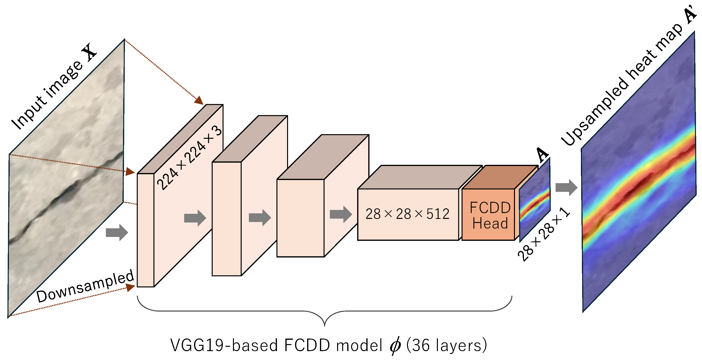
Figure 3.
Examples of training results. (a) is completely trained case, in which normal and anomaly samples in training dataset are completely separated. (b) is not-completely trained case, in which overlaps of normal and anomaly bins are seen.
Figure 3.
Examples of training results. (a) is completely trained case, in which normal and anomaly samples in training dataset are completely separated. (b) is not-completely trained case, in which overlaps of normal and anomaly bins are seen.
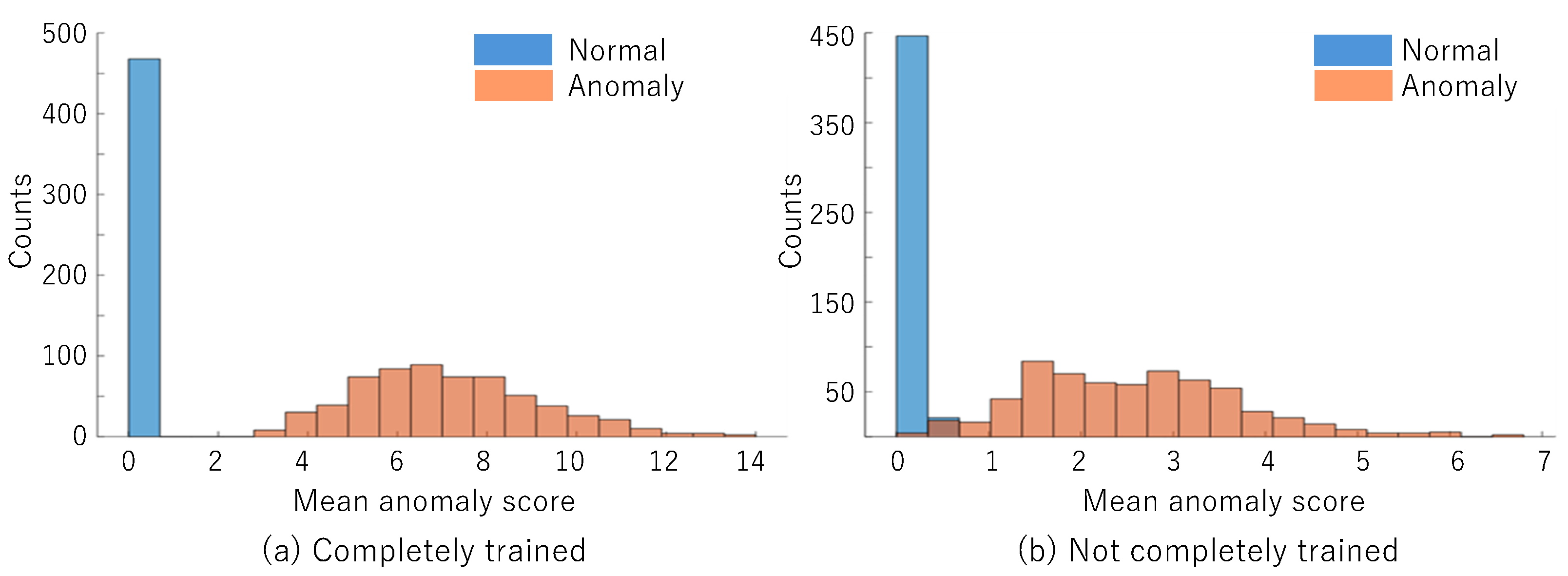
Figure 4.
Examples of brake rotors without defects [8].
Figure 4.
Examples of brake rotors without defects [8].
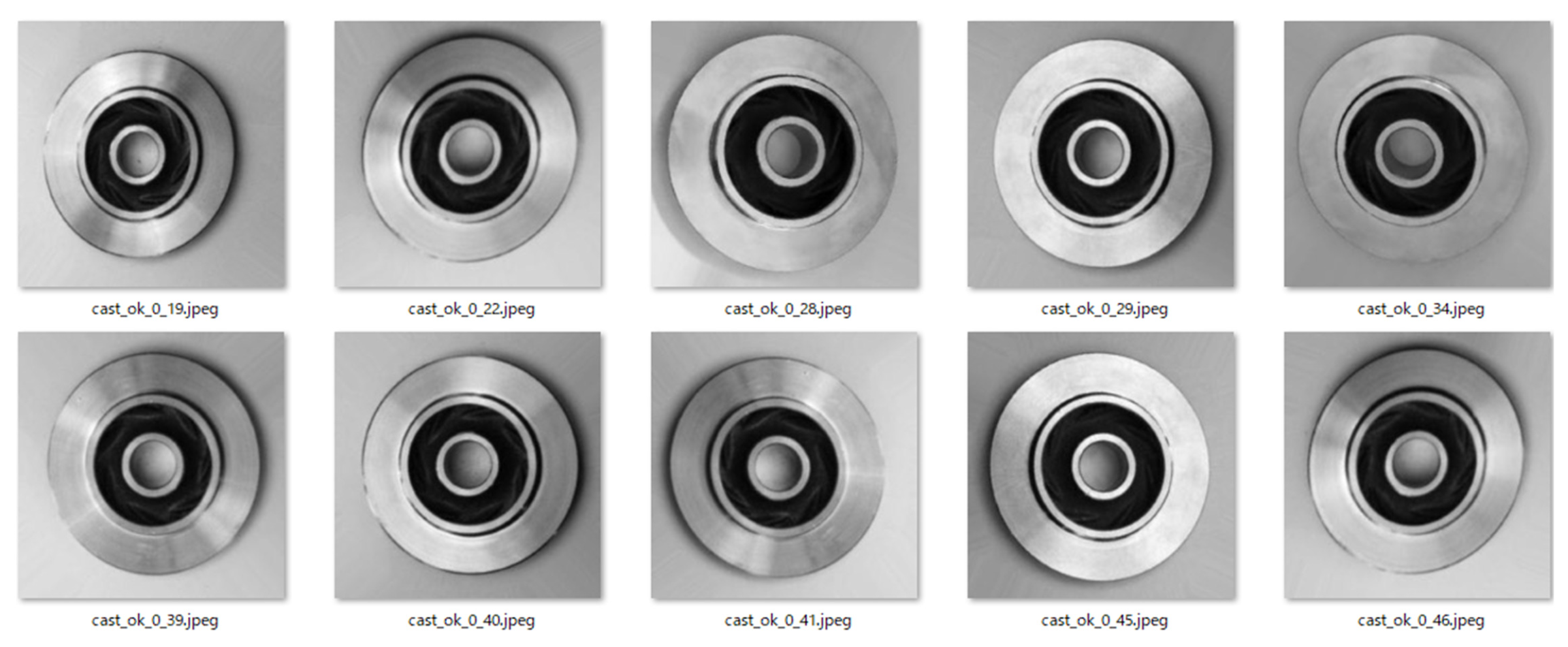
Figure 5.
Examples of brake rotors with defects [8].
Figure 5.
Examples of brake rotors with defects [8].
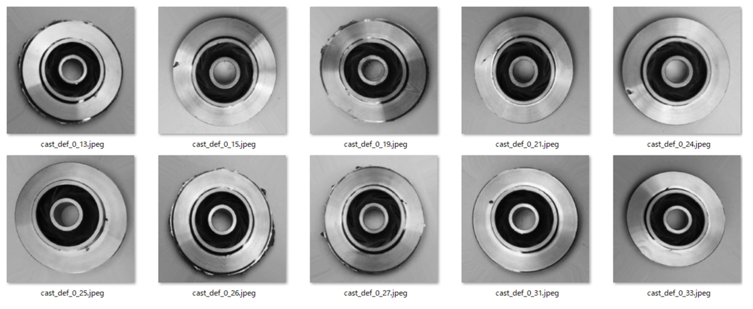
Figure 6.
Only one misclassified image named `cast_def_0_571.jpeg’ (False Negative).
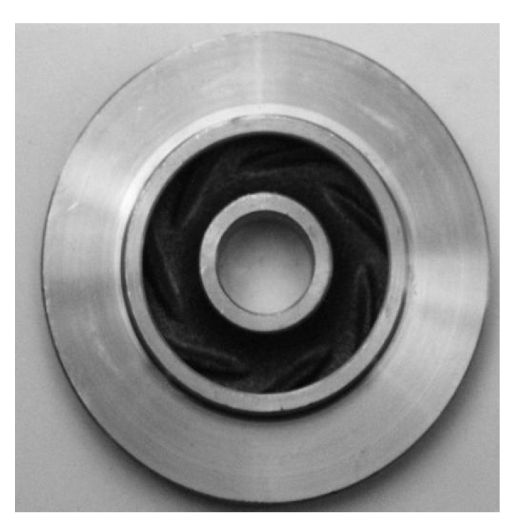
Figure 7.
Heat maps generated by Grad-CAM.
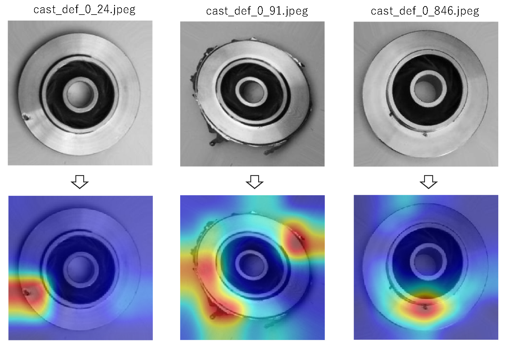
Figure 8.
Heat maps generated by Occlusion Sensitivity.
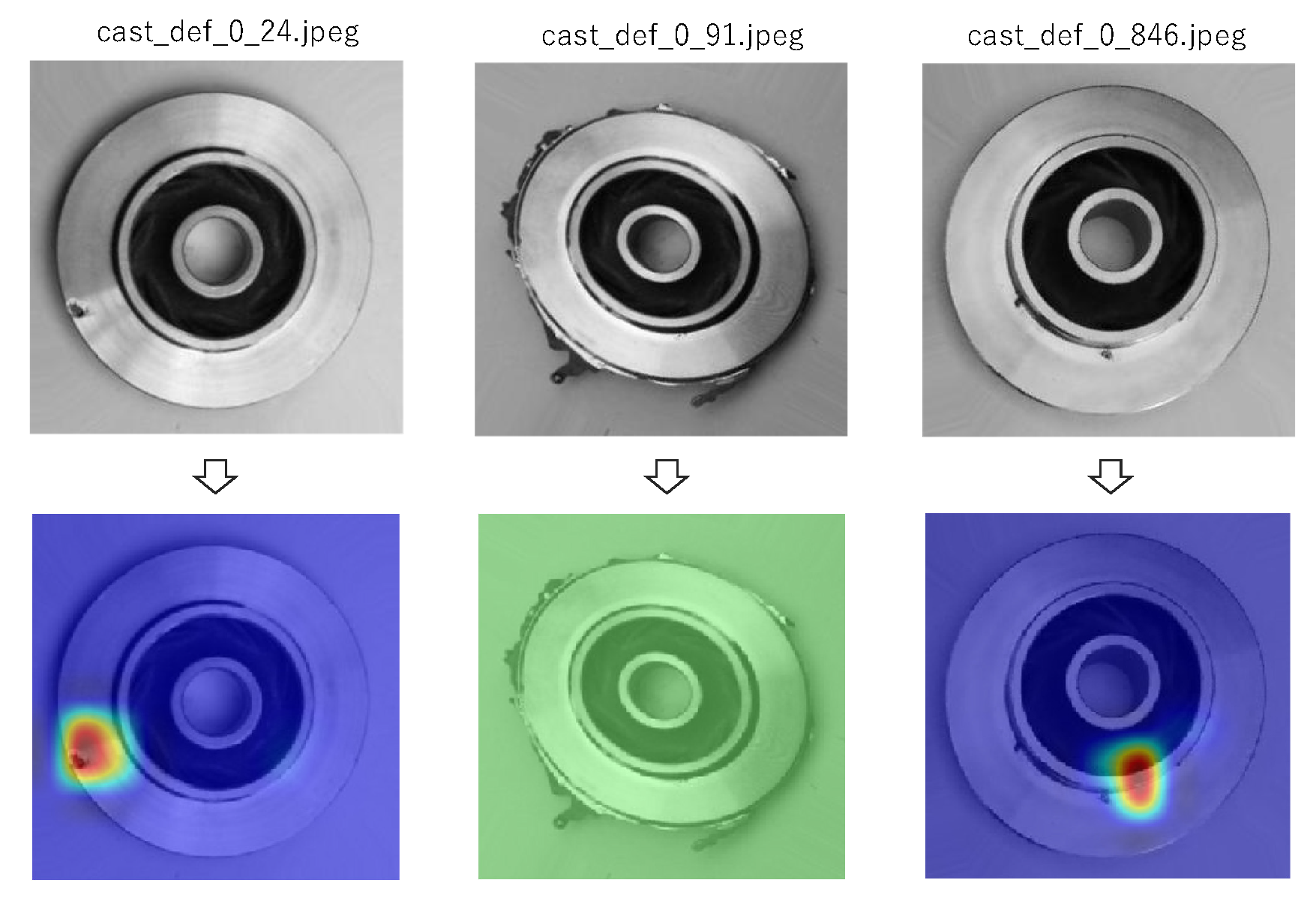
Figure 9.
More reasonable and clearer heat maps generated by FCDD than Grad-CAM and Occlusion Sensitivity.
Figure 9.
More reasonable and clearer heat maps generated by FCDD than Grad-CAM and Occlusion Sensitivity.
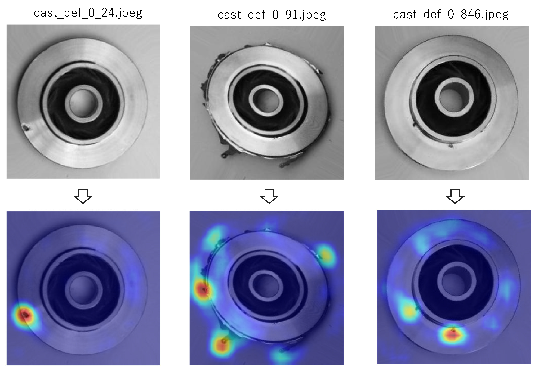
Figure 10.
Examples of original (upper) and enlarged (lower) images of fibrous industrial material without defects.
Figure 10.
Examples of original (upper) and enlarged (lower) images of fibrous industrial material without defects.
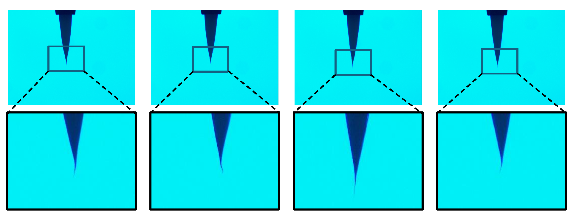
Figure 11.
Examples of original (upper) and enlarged (lower) images of fibrous industrial product with defects. Split-hair type and frayed type defects are seen.
Figure 11.
Examples of original (upper) and enlarged (lower) images of fibrous industrial product with defects. Split-hair type and frayed type defects are seen.
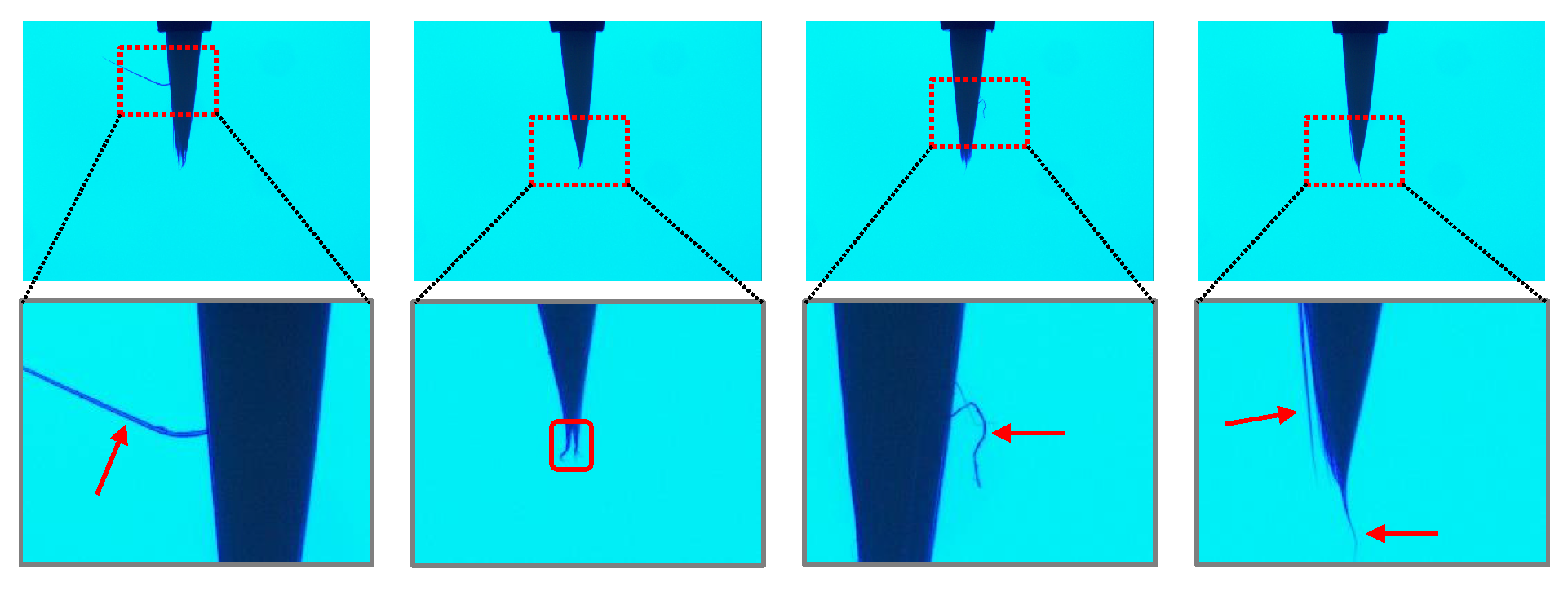
Figure 12.
Downsizing process to fit the input layer of VGG19. There is a concern that features of small and thin defects may be lost.
Figure 12.
Downsizing process to fit the input layer of VGG19. There is a concern that features of small and thin defects may be lost.
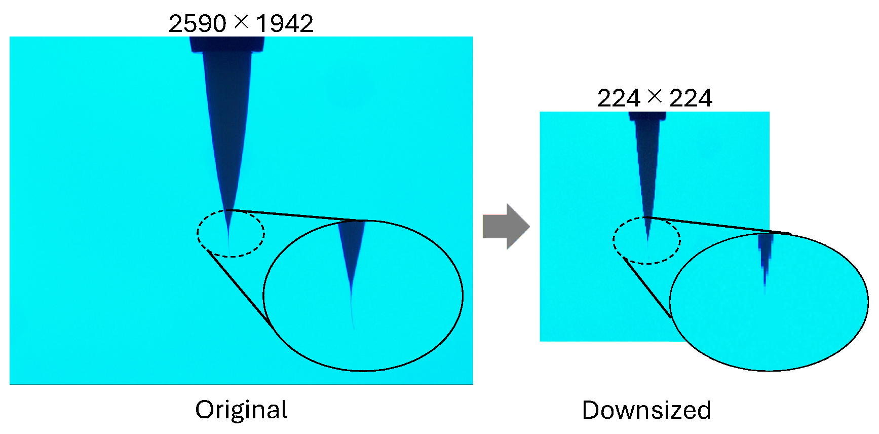
Figure 13.
Heat maps generated by Grad-CAM, in which the split-end type defect is not heatmapped.
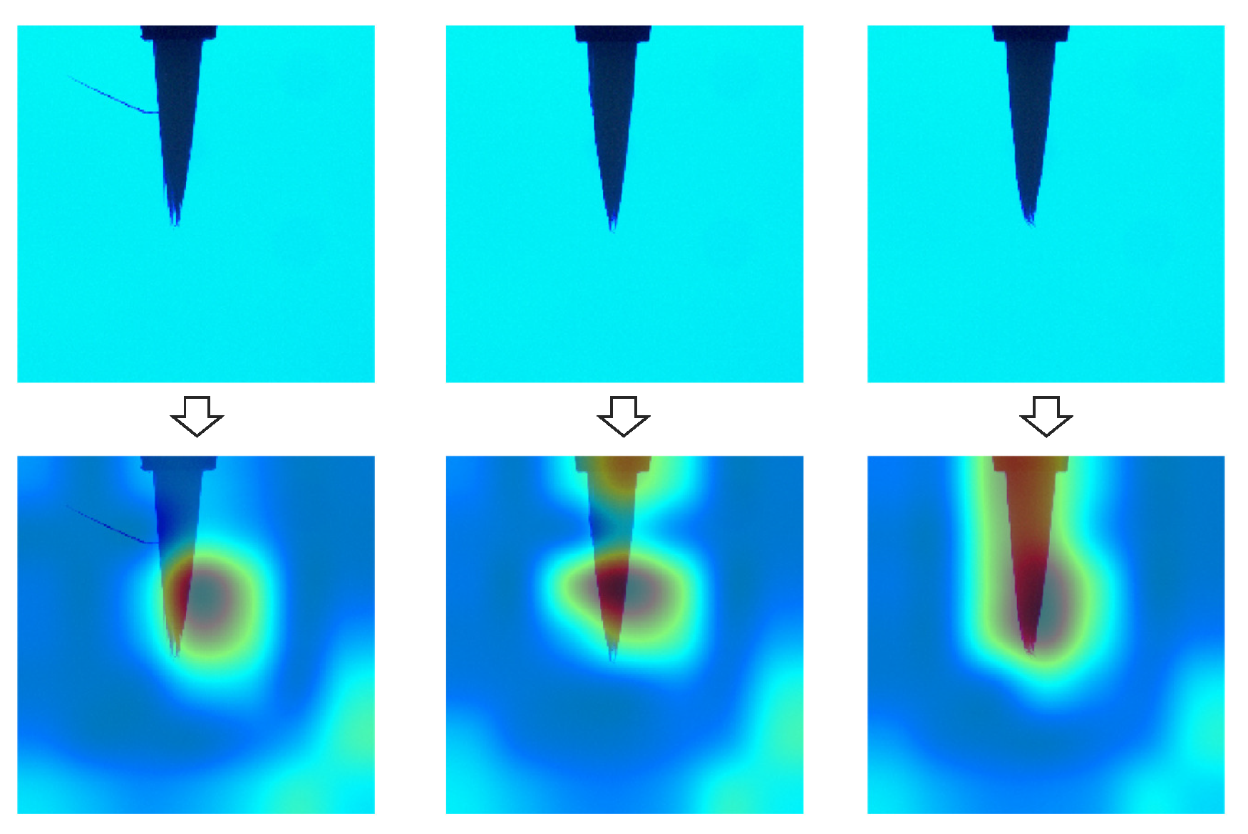
Figure 14.
Heat maps generated by Occlusion Sensitivity appear to be better than Figure 13, however, the split-hair type defect in left side photo is not still heatmapped.
Figure 14.
Heat maps generated by Occlusion Sensitivity appear to be better than Figure 13, however, the split-hair type defect in left side photo is not still heatmapped.
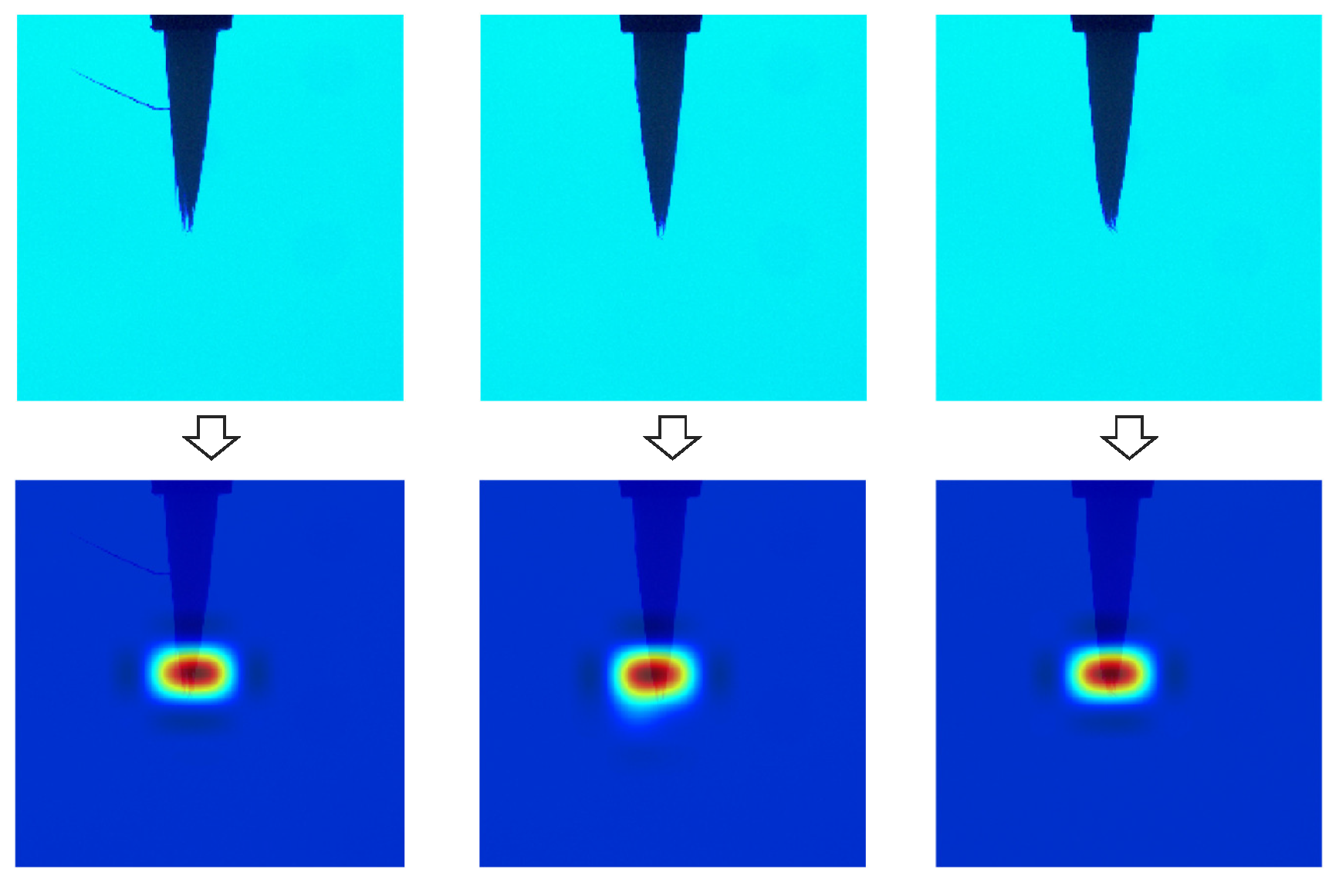
Figure 15.
Heat maps generated by FCDD, in which even the split-hair type defect is successfully heatmapped.
Figure 15.
Heat maps generated by FCDD, in which even the split-hair type defect is successfully heatmapped.
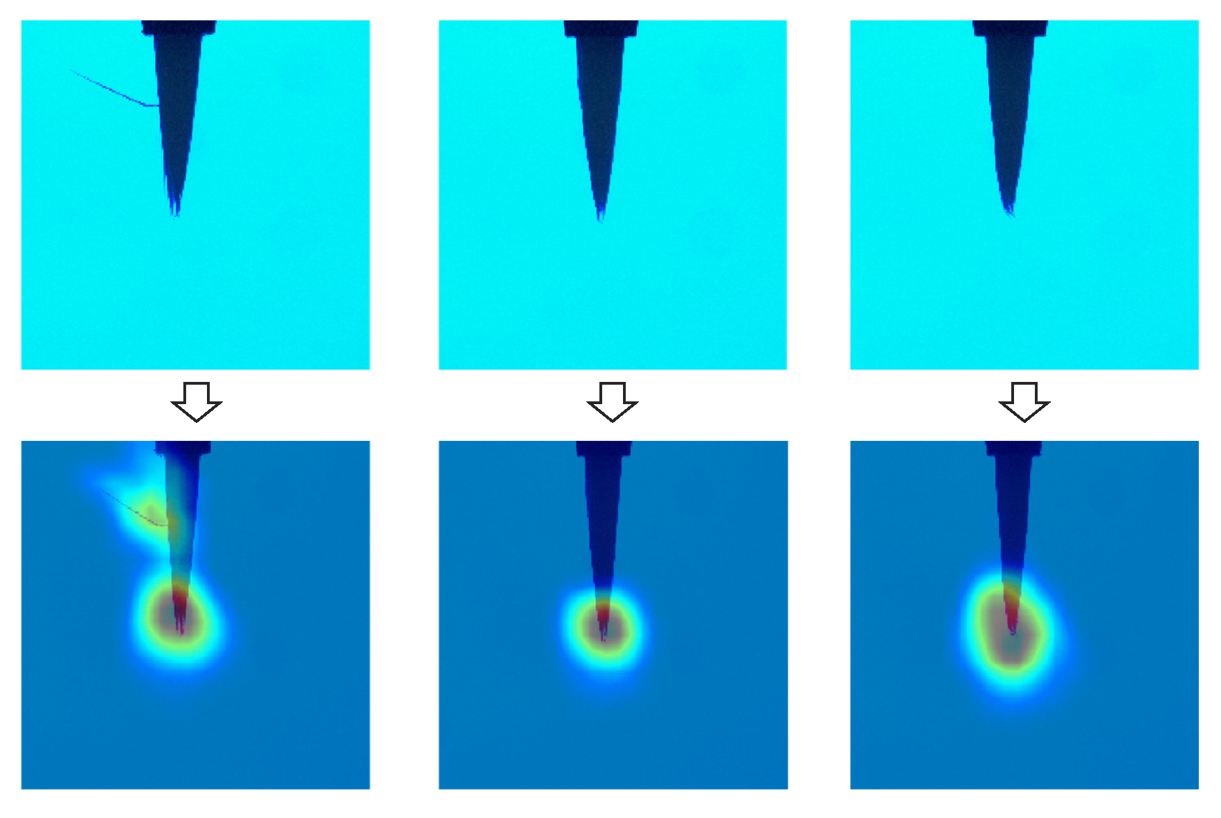
Figure 16.
Image samples of wrap films on production line before extraction by template matching.
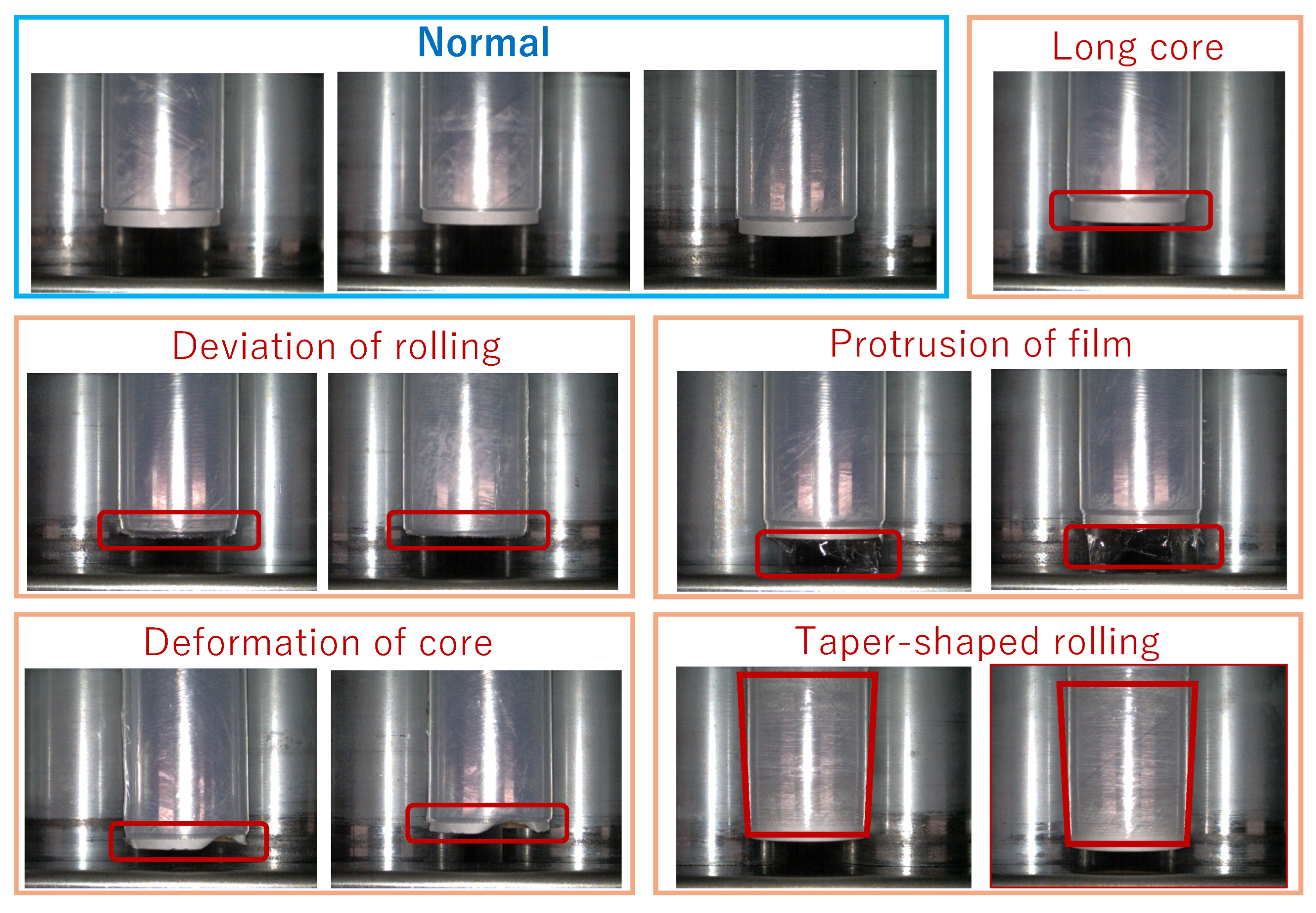
Figure 17.
Heat maps generated by Grad-CAM.
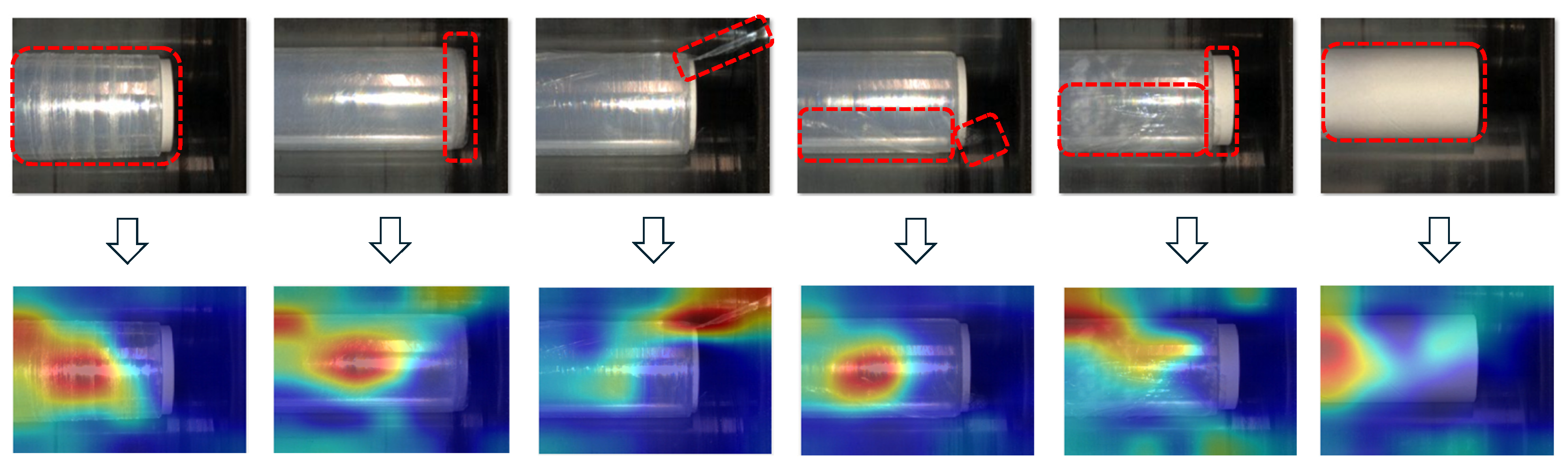
Figure 18.
Heat maps generated by Occlusion Sensitivity.
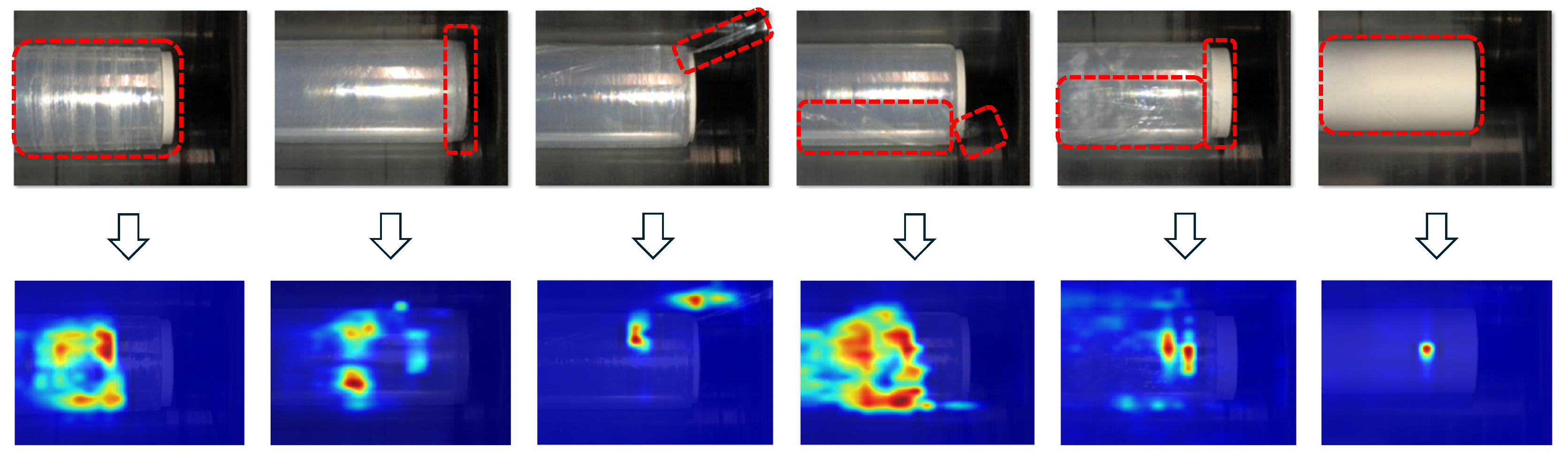
Figure 19.
Heat maps generated by FCDD.
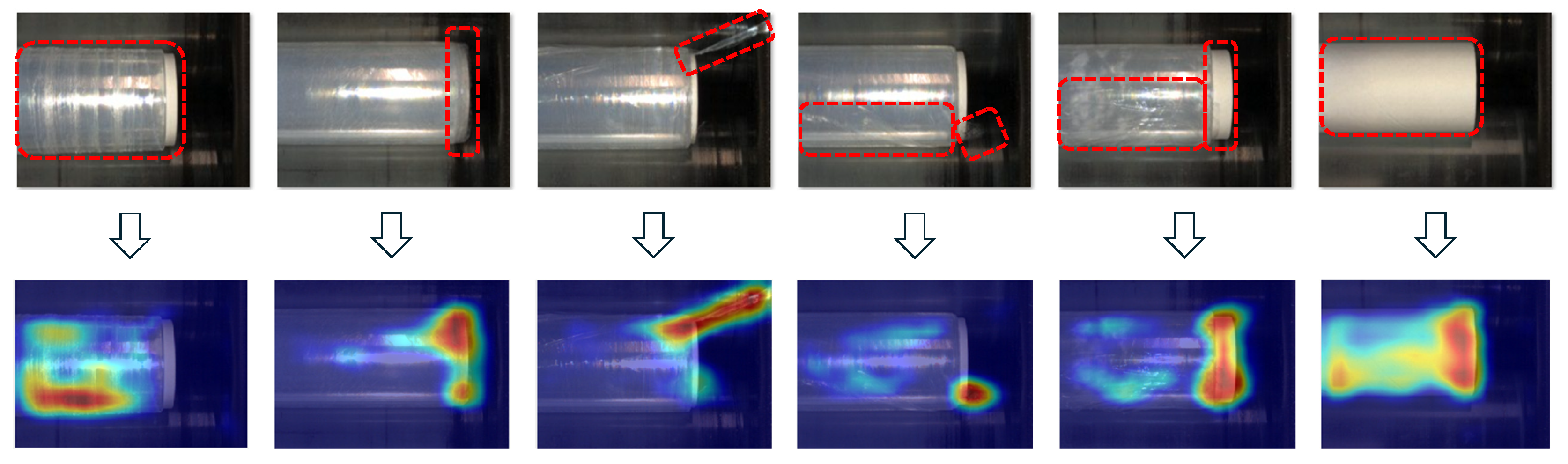

Table 1.
Classification result by VGG19-based CNN.
| Predicted | Anomaly (NG) | Normal (OK) | |
|---|---|---|---|
| True | |||
| Anomaly (NG) | 99 | 1 | |
| Normal (OK) | 0 | 100 | |
Table 2.
Classification result by FCDD model (threshold=0.53).
| Predicted | Anomaly (NG) | Normal (OK) | |
|---|---|---|---|
| True | |||
| Anomaly (NG) | 99 | 1 | |
| Normal (OK) | 0 | 100 | |
Table 3.
Classification result by VGG19-based CNN.
| Predicted | Anomaly (NG) | Normal (OK) | |
|---|---|---|---|
| True | |||
| Anomaly (NG) | 50 | 5 | |
| Normal (OK) | 5 | 41 | |
Table 4.
Classification result by FCDD model (threshold=1.30).
| Predicted | Anomaly (NG) | Normal (OK) | |
|---|---|---|---|
| True | |||
| Anomaly (NG) | 50 | 5 | |
| Normal (OK) | 6 | 40 | |
Table 5.
Classification result by VGG19-based CNN.
| Predicted | Anomaly (NG) | Normal (OK) | |
|---|---|---|---|
| True | |||
| Anomaly (NG) | 618 | 10 | |
| Normal (OK) | 23 | 445 | |
Table 6.
Classification result by FCDD model (threshold=1.50).
| Predicted | Anomaly (NG) | Normal (OK) | |
|---|---|---|---|
| True | |||
| Anomaly (NG) | 620 | 8 | |
| Normal (OK) | 11 | 457 | |
Disclaimer/Publisher’s Note: The statements, opinions and data contained in all publications are solely those of the individual author(s) and contributor(s) and not of MDPI and/or the editor(s). MDPI and/or the editor(s) disclaim responsibility for any injury to people or property resulting from any ideas, methods, instructions or products referred to in the content. |
© 2025 by the authors. Licensee MDPI, Basel, Switzerland. This article is an open access article distributed under the terms and conditions of the Creative Commons Attribution (CC BY) license (http://creativecommons.org/licenses/by/4.0/).
Copyright: This open access article is published under a Creative Commons CC BY 4.0 license, which permit the free download, distribution, and reuse, provided that the author and preprint are cited in any reuse.


