Submitted:
22 January 2025
Posted:
22 January 2025
You are already at the latest version
Abstract
The industrial application of artificial intelligence (AI) has witnessed outstanding adoption due to its robust efficiency in recent times. Image fault detection and classification have also been implemented industrially for product defect detection, as well as for maintaining standards and optimizing processes using AI. However, there are deep concerns regarding the latency in the performance of AI for fault detection in curvy and glossy products, due to their nature and reflective surfaces, which hinder the adequate capturing of defective areas using traditional cameras. Consequently, this study presents an enhanced method forcurvy and glossy surface image data collection using a Basler vision camera with specialized lighting and KEYENCE displacement sensors, which are used to train deep learning models. Our approach employed image data generated from normal and two defect conditions to train eight deep learning algorithms: four custom Convolutional Neural Networks (CNNs), two variations of VGG-16, and two variations of ResNet-50. The objective was to develop a computationally robust and efficient model by deploying global assessment metrics as evaluation criteria. Our results indicate that a variation of ResNet-50, ResNet-50224, demonstrated the best overall efficiency, achieving an accuracy of 97.79%, a loss of 0.1030, and an average training step time of 839 milliseconds. However, in terms of computational efficiency, it was outperformed by one of the custom CNN models, CNN6-240, which achieved an accuracy of 95.08%, a loss of 0.2753, and an average step time of 94 milliseconds, making CNN6-240 a viable option for resource-sensitive environments.
Keywords:
Convolutional neural network
; residual neural network-50
; visual geometry group 16 layers
; Dijkstra’s algorithm
; curvy surface
; reflective surface
; fault classification
; fault detction
1. Introduction
Over the years, the manufacturing sector has undergone a remarkable transformation since the introduction of Industry 4.0, as it has uniquely revolutionized industrial operations by leveraging smart technological implementations, which have enhanced and fostered global innovation and competitiveness in the manufacturing sector. AI has been used not only in manufacturing processes but has also played a crucial role in the maintenance and reliability of industrial machinery. The aspect of AI known as Prognostics and Health Management (PHM) has ensured that production remains uninterrupted by monitoring the life and performance of a system. PHM enables real-time monitoring and assessment of systems, as it has the capacity to monitor a system both online (while in operation) and offline (when not in operation) [1]. It can predict the current and future state of a given system based on information generated through sensor technology. Notwithstanding that PHM originated in the the aerospace industry, its tentacle has spread and has been explored in industries such as manufacturing, energy, production, automotive, construction, textile, healthcare, and pharmaceutical industries.
In light of this, vision-based analysis has been successfully employed in manufacturing for standard and quality product control inspections [2]. Image fault detection has also been efficiently implemented in technical fields such as intelligent traffic monitoring and unmanned aerial vehicles [3,4]. Nonetheless, even though there have been recorded success rates and efficiencies of PHM models in system diagnostics and monitoring, researchers are often tasked with the responsibility of developing and enhancing condition-based system models. These models aim to increase the efficiency and robustness of existing methodologies or address challenging issues unresolved by current models. One such challenge is often encountered in automated defect inspection and machine vision-based fault detection when dealing with glossy surfaces and glossy-curvy surface defect detection. This issue can be attributed to the complex reflectiveness of glossy surfaces and the curvy morphological nature of these surfaces, which often cause defects to go unnoticed when captured by traditional cameras [5,6]. Over the decades, inspection and defect detection of issues such as cracks, scratches, dents, etc., in such scenarios have been performed manually by professional human quality inspectors. These inspectors, who are thoroughly trained and specialized in quality control, have been solely responsible for curvy and glossy surface quality inspection and defect detection, rather than relying on automated processes. This manual inspection approach is not only time consuming but also monetarily expensive compared to non-glossy surface inspection and defect detection processes, which are fully automated [5,7].
In recent times, researchers have mainly tackled these challenges by focusing on developing unique image processing techniques to improve image quality for better model interpretation. Additionally, they have enhanced deep learning architectures to enable models to learn and understand the nature of images, even in complex states [8,9,10]. However, most studies report situations where the intensity of the reflection or real-life application of the model does not perform as required or expected. Furthermore, even when the model performs well with a given dataset, it often fails to achieve the same results when tested on datasets with varying levels of reflectiveness. For instance, the authors in [11] proposed a methodology to detect glass defects in real environments by focusing on the characteristics of the semi-mirror surface. Although their methodology was able to detect and classify faults on both the glass itself and in its own reflection-cast image, it faced difficulties when the background image and the reflected image had a high level of similarity.
Another alternative approach used in image fault detection for glossy and curved surfaces is to modify the techniques used to capture these images and employ advanced cameras with enhanced lighting systems, which can effectively reduce the reflective properties of the surfaces. Techniques such as polynomial texture mapping, surface-enhanced ellipsometry, specular holography, and near-field imaging have been explored in studies [12,13,14]. However, some reported limitations include environmental factors that can affect performance, the inability of certain techniques for all types of surface, and the potential reduction in image resolution [10,11,15]. Alternatively, some of these limitations can be mitigated by employing advanced image augmentation and image processing techniques in combination with robust deep learning-based image detection architectures, such as Convolutional Neural Networks (CNNs) and their subsidiary architectures, including VGG-16, ResNet-50, YOLO, and Mask R-CNN [16,17]. Furthermore, the search for better alternatives remains ongoing, encouraging researchers to explore and develop more advanced models.
Product quality inspection is an indispensable aspect of the manufacturing and production sector, as maintaining a given standard ensures quality and meets customers’ tastes and expectations. Methodologies such as visual inspection, which involves trained human experts manually inspecting products, and automated optical inspection (AOI), which employs high-resolution cameras and image processing algorithms tuned to identify defects, are widely used [18,19,20]. Other methodologies include machine vision, infrared thermography, laser scanning and profiling, and X-ray inspection, among others.
Of all these methodologies, computer vision has gained the most relevance, particularly as the global technological landscape increasingly embraces AI and transitions gradually from Industry 4.0 to Industry 5.0. Its high precision, computational efficiency, non-contact nature, and excellent performance, when executed properly, also make it stand out [21,22]. As a result, some of the mentioned methodologies, such as manual inspection, are becoming obsolete and witnessing diminished reliance. However, applying certain methodologies still faces barriers that limit their utility and efficiency with specific surfaces. Glossy and curved surfaces, in particular, pose challenges for adopting machine vision technology due to their reflectivity and uneven illumination, which often make defect detection inconsistent [6]. As a result, visual inspection remains a relevant technique in these instances. From a broader perspective, one may argue that machine vision might be expensive to set up, but upon deeper assessment, its expense is a one-off event that provides long-term benefits, as long as the model remains efficient and does not require retraining. In contrast, visual inspection, which might initially seem a cheaper option, incurs recurring costs since a fee is required for each new batch of products that need inspection.
This has prompted researchers continuous development of techniques to address these challenges, ensuring the seamless implementation and application of AI-powered techniques in this spectrum. The motivation for this study lies in the urgent need to develop a classification model for glossy and curved surfaced products in a manufacturing company. Figure 1 provides an overview of the product sample: a uniquely designed hairbrush case cover tailored for women. This product combines aesthetic appeal with practical functionality, addressing a specific need for women. Its uniqueness lies not only in its design but also in its ergonomic nature, material composition, and ability to fit comfortably in the palm. Additionally, it plays a significant role in extending the lifespan of the hairbrush by offering protection and convenience. Its versatile design makes it suitable for a variety of occasions and uses.
However, the aesthetic nature of this product not only attracts patronage but also presents some challenges. The glossy and curved design of this product adapts traditional machine-vision inspection techniques an issue. Quality inspection for this product is of utmost importance, given the demographic it is made for, which demands that anything less than the best will be rejected. This has also influenced online platforms to reject these products when defects such as cracks, dents, and scratches are detected. In the past and present, research often employs two major approaches to address such challenges. The first involves introducing techniques or cameras designed to reduce the surface reflectiveness, allowing a clearer view of the image [23,24]. However, some might argue that this methodology could be expensive and may not provide a detailed overview of the product sample.
For instance, Müller, in his study, employed polarization filters to reduce surface reflectiveness, which provided enhanced clarity to the image. He achieved this by capturing two images with different orientations of the polarization filter from a camera and then deriving the intensity of specular reflectance on the plane surfaces. This method, he stated, effectively mitigated the impact of surface reflections [25]. Similarly, in another study [24], Yoon et al. presented a technique for removing light reflections in medical diagnostic imaging by adjusting the angle of a linear polarized filter. They accomplished this by controlling the image’s vertical and horizontal polarization through filter rotation. According to their findings, this method effectively removes light reflections during the imaging process, thereby enhancing the field of view of the surface.
The second technique often employed involves implementing advanced algorithms and deep learning models that are robust enough to handle glossy surfaces by learning and extracting pertinent features and information to achieve detailed analysis and desired outcomes. As an example, the authors in [26] introduced a novel spatial augmented reality framework to enhance the appearance of glossy surfaces. Their technique involved spatially manipulating the appearance of an environment observed through specular reflection. According to the authors, this method allowed a glossy surface to reflect a projected image, enabling the alteration of its appearance without direct modification. This approach, they asserted, enables effective appearance editing of glossy surfaces by carefully controlling the projected content. Similarly, in a separate study [27], Yuan et al. proposed a dual-mask-guided deep learning model specifically designed to detect surface defects on highly reflective leather materials. They concluded that their model enhances the accuracy of defect detection on glossy surfaces by effectively removing surface specular highlights in images while preserving bright defects. Though leather surfaces might not be regarded as perfectly reflective, the technique could be assumed to work effectively on highly glossy surfaces when implemented properly using robust models.
Irrespective of the technique employed to ensure a robust defect detection model, the nature of the classifier or fault detection algorithm used is of utmost importance. One of the most robust deep learning algorithms in artificial neural networks is the convolutional neural network (CNN). CNNs have dominated the field of computer vision since their remarkable performance in the ImageNet Large Scale Visual Recognition Competition in 2012. They have been successfully deployed in various fields, such as medical imaging, where they have been used to detect tumors and other irregularities with higher accuracy, as well as for fault detection using MRI and X-ray images [28,29,30]. Notable examples in recent studies can be seen in the work of Rajeshkumar et al. [31], which highlighted the utilization of CNNs in the diagnosis of brain tumors using MRI scans, emphasizing the importance of prompt and efficient response in defect detection in medical practice. The application of CNNs was further demonstrated in their study through their methodology, which showcased the flexibility of CNNs. They adopted a grid search optimization technique to enhance the performance of three different CNN models for multi-classification tasks involving brain tumor images. Although the three CNN models displayed varying levels of performance, they highlighted the diversity and adaptability of CNNs in task implementation. Their models achieved high accuracy in identifying and classifying various types of brain tumors, further showcasing the reliability and effectiveness of CNNs in medical image analysis.
Over the years, Convolutional Neural Networks (CNNs) have evolved into numerous specialized architectures to address specific challenges in computer vision tasks, including segmentation, object detection, fault detection, and beyond. For instance, the Visual Geometry Group (VGG) architecture is a standard CNN model with multiple layers that emphasizes simplicity by employing deep sequential layers, enabling improved feature extraction [32,33]. However, this comes at a high computational cost due to its depth. The Residual Neural Network (ResNet) architecture revolutionized deep networks by introducing residual connections, which mitigate the vanishing gradient problem and enable the development of much deeper architectures [34].
The robustness of ResNet was demonstrated in this study [35]. The authors compared traditional CNN architectures, including Inception V3, VGG-16, VGG-19, and a conventional CNN, for early fault detection of rice leaf blast disease. Their results showed that ResNet-50 achieved the best accuracy of 99.75%, highlighting the importance of deep feature extraction in agricultural applications. Similarly, the authors in another study [36], utilized the robustness of a CNN sub-type to achieve their desired goal. In their implementation, a COVID-19 detection and classification model was developed using Faster R-CNN with a VGG-16 backbone to detect and classify COVID-19 infections in computed tomography (CT) images. This model achieved an accuracy of 93.86%, further demonstrating the effectiveness of region-based CNNs in medical image analysis.
Another key concern over the years in image fault detection is detecting faults on curved surfaces, which presents a significant challenge for fixed cameras. Among various suggested methodologies and techniques, the robotic arm has proven to be effective due to its flexibility, allowing for easy navigation through curvatures. Wang et al. emphasized its effectiveness in their study [37], where they employed a robotic arm equipped with a 3D micro X-ray fluorescence (µXRF) spectrometer and a depth camera to achieve high-precision scanning of curved surfaces. They stated that this setup ensured the consistency of the X-ray incident angle and scanning distance, minimizing counting errors and thus improving accuracy. The robot’s flexible six-axis design allows for comprehensive surface inspections from various perspectives, enhancing the system’s capability in industrial applications. Similarly, Huo, Navarro-Alarcon, and Chik demonstrated the importance of utilizing robotic arms in their study [38]. They developed an inspection model using a six-degree-of-freedom manipulator equipped with a line scan camera and high-intensity lighting. This setup, they highlighted, enabled inspections of convex, free-form, specular surfaces by adapting the region of interest, thereby ensuring and enhancing defect detection capabilities on complex geometries.
To ensure that fault classification is effectively carried out on glossy and curved surfaces in the manufacturing industry, this study makes the following contributions:
- Proposed the integration of a Basler Vision camera with enhanced lighting to achieve high-quality image acquisition of glossy surfaces, thereby facilitating the development of a robust fault detection and classification framework.
- Proposed the utilization of a KEYENCE Laser displacement Sensor equipment in combination with a Motoman-GP7 Yankawa robotic arm to enable the effective acquisition of curvy geometries.
- Proposed a comparative assessment of robust deep learning algorithms for image-based fault detection, with global assessment metrics such as accuracy, loss, computational efficiency, recall, F1 score, specificity, mAP, and confusion matrix, to validate the performance of our model and identify an efficient algorithm that requires less computational energy.
The rest of the paper is structured as follows: Section 3 explains the theoretical background of the core techniques employed in the study. Section 4 provides details on the experimental setup and methodologies used to achieve the study’s objectives. Section 5 presents an evaluation of the model’s performance, while Section 6 and 7 discuss the study’s results and conclusions, respectively.
2. Theoretical Background
This section discusses the theoretical background of CNN architecture and its sub-types as employed in the study. It also explores key techniques utilized in the development of the proposed framework.
2.1. Convolutional Neural Network
Convolutional Neural Networks (CNNs), also refered to as ConvNets, are a unique class of artificial intelligence systems structured with a multi-layer neural network architecture. They have been efficiently applied to various tasks, including identification, recognition, and classification, as well as detection and segmentation. CNNs have also been successfully implemented in fields such as natural language processing, speech recognition, time series analysis, image classification, and vision-based fault detection [39,40]. Their capability to learn directly from input data, without the need for manual feature extraction, makes them highly efficient. This efficiency is attributed to their discriminative deep learning architecture, which enables them to perform complex tasks with minimal human intervention.
The concept of CNN was first introduced in the 1950s and 1960s by Hubel and Wiesel during their study of the stimuli in the visual cortex of cats, where they investigated the hierarchical representation of neurons. However, CNNs gained significant popularity in 2012 following their breakthrough in the ImageNet Large Scale Visual Recognition Competition [39,41]. CNNs are generally categorized based on the dimensionality of their input structure: one-dimensional (1D), two-dimensional (2D), and three-dimensional (3D). 1D CNNs specialize in sequential data such as audio and time series. 2D CNNs excel in image-related tasks, including image segmentation, classification, and detection. 3D CNNs handle volumetric datasets, such as CT scans and videos [42,43,44]. Each of these categories employs specialized kernels to extract relevant features based on the presented task. CNNs have been successfully applied in models for fault detection, computer vision, and signal processing.
2.1.1. CNN Architectural Overview
A typical CNN architecture is composed primarily of six-layer namely:
- Input layer
- Convolutional layer
- Pooling layer
- Flatten layer
- Fully connected layer
- Output layer
The pictorial illustration of the CNN layers is shown in Figure 2. A CNN is composed of unique layers, each performing a specific task, which collectively makes it a standout algorithm. Understanding its architecture is paramount to ensuring proper implementation and achieving the desired output. In this overview, our core focus will be on image understanding tasks, which include processing, classification, and fault detection using CNNs (Conv2D).
The first layer of a Convolutional Neural Network (CNN) is the input layer, which determines the nature and form of the input based on the task the CNN is configured to perform. In an image input scenario, the building blocks of computer vision are structured in pixels. Pixels represent the numerical equivalents of each color grade, typically ranging from 0 to 255 [39]. Each color in an image is graded based on this scale, which helps to sequentially organize image inputs into a matrix format. This matrix format transforms the image into a digital layout that the CNN can process. For a comprehensive understanding of the image structure, the brightness, shade, and tint of the image pixels are determined by their pixel value grading [39,40].
Input layer: The input layer of the CNN is crucial as it determines and maintains the nature of the input, which directly influences the performance and efficiency of the model. This layer defines the format and structure of the raw data input. To ensure optimal performance of the overall model, factors such as image resolution, data augmentation, normalization, and input channels must be addressed to align with the format of the input layer [45]. The input layer recognizes three input channel formats: (1) grayscale, (3) RGB (red, green, blue), and (4) alpha channel (RGBA, where A represents transparency). Augmentation helps prepossess the image to enable the CNN model to learn and extract the required features for optimal performance [46].
To normalize a given image’s pixel values for an input instance, each pixel intensity , where x, y, and c represent the height, width, and channel of the image pixel, is divided by 255. This process scales the pixel values from the range 0–255 to a normalized range of 0–1. This normalization ensures consistency across the dataset, thereby maintaining stability during the training of the CNN model. Mathematically, image pixel value normalization can be represented as shown in Equ. 1:
Where stands for the normalized image pixel value, I presents the original pixel value.
The output of the input layer, fed to the convolutional layer, is known as a tensor. This tensor is interpreted by the convolutional layer for further processing and feature extraction.
Convolutional layer: The convolutional layer is a unique and pivotal component of the CNN architecture, primarily responsible for feature extraction. It comprises multiple sub-layers that work simultaneously to process the tensor and extract useful features such as edges, textures, and corners. Its working principle involves filters (also known as kernels), which are small matrices of learnable weights [47]. These filters convolve through the input array, performing a dot product operation with specified strides, ultimately producing a feature map.
At each given position, an element-wise multiplication is performed between the filter values and the corresponding pixels of the input image. The results are then summed up. For a given normalized image pixel fed to a kernel K, the equation of the convolution operation in the convolutional layer is presented in Equation 2.
Where stands for the output values at positions i and j in the th feature map. U, V, and V represents the filter’s height, width, and input channels receptively, stands for the filter weight at positions u and v for the c-th channel of the k-th filter, and is bias.
The filter size determines the level of details captured in a given image input. Traditionally, filter sizes are often 3×3, 5×5, and 7×7, and the choice is typically based on the user’s preference. Convolutional layers are commonly stacked to ensure detailed feature extraction. Primarily, the first layer extracts low-level features such as edges and corners, while the mid-level layers extract intermediate features such as shapes and patterns. Deeper layers focus on extracting high-level features, which are essential for a comprehensive understanding of distinct and complex patterns. Stacking ensures a progressive increase in the neuron receptive field and allows the network to learn hierarchical representations, which are crucial for complex tasks [48]. Filters, which are learnable weights that extract features, determine the number of different features learned by the network in a given stacked layer. The network learns the weights of these filters during training, adapting to recognize specific features [39].
For instance, a layer with 16 filters will generate 16 feature maps, each corresponding to a different learned feature. The size of the kernel determines the level of detail captured; smaller filters capture finer details, while larger filters capture more context but are more computationally expensive. Strides and padding are other important features of the convolutional layer, as they significantly influence the nature of the convolutional layer’s output [49]. Strides control the step size of the filter during convolution; a stride of 1 ensures that all pixels are processed. However, a stride greater than 1 might not capture all the pixels and will reduce the spatial dimensions of the output.
On the other hand, padding determines the inclusion of input edges in the convolution computation. For instance, padding adds zeros around the input pixels, resulting in an output with the same spatial dimensions as the input. padding, on the other hand, does not pad with zeros, resulting in a smaller output due to the reduction caused by the kernel’s dimensions [45,49].
Pooling layer: The pooling layer, also called downsampling, helps to refine the extracted features from the convolutional layer by reducing the dimensionality of the feature map. While performing this reduction, it retains the most significant features, thereby enhancing the network’s performance [39,45]. This ensures the model maintains its accuracy and computational efficiency. The pooling layer employs three types: max pooling, average pooling, and global pooling. Max pooling selects the strongest feature (maximum value) in a given pooling window. Average pooling, on the other hand, computes the average value in the pooling window. Global pooling operates by applying max or average pooling over the entire feature map, reducing it to a single value per channel [39,50].
However, for pooling to be implemented, the pooling window size must be determined, as it defines the dimension of the region over which the pooling operation can be applied to the feature map. This determines the nature of the downsampling in a given pooling layer. Hence, selecting an appropriate window size is paramount in determining the quality and nature of the downsampling performed by the pooling layer. For instance, smaller window sizes, like 2×2, retain finer details of feature maps while downsampling. Larger windows, such as 3×3, offer a more aggressive dimensional reduction, which might lead to the loss of fine details. However, their advantage lies in their ability to capture more contextual features compared to smaller window sizes.
Additionally, while the window size is crucial, the stride is also important as it controls the movement of the pooling window during the pooling operation, similar to its role in the convolutional layer. The stride has a direct impact on the dimensions of the pooling layer’s output. Larger strides result in greater dimensional reduction, whereas smaller strides retain more spatial details in the output feature map. Mathematically, the output of the pooling layer can be represented as follows:
where represents the output and its dimensions, represents the input and its dimensions, and stands for the pooling window and its dimensions. P and S represent padding and strides, respectively.
In addition to Equation 3, the equations for max pooling and average pooling are shown below in Equations eqm,eqa, respectively.
Flatten layer: This layer’s functionality is pivotal as it serves as a bridge between the convolutional layer, through the pooling layer, to the fully connected layer. Its core function is to transform the multidimensional feature map input from the pooling layer into a one-dimensional vector, enabling easier feature processing for the fully connected layer without loss of information [51,52]. For instance, if the output from the pooling layer is of size 3 × 3 with 64 feature maps, the flattening layer reshapes the output into a one-dimensional vector of size 3 × 3 × 64 = 576. This format is compatible with the fully connected layer, helping the CNN achieve its output by transitioning from multi-dimensional features to a final decision.
Fully connected layers and output layer: The fully connected layer, also known as the dense layer, is a layer in a neural network that functions by connecting every neuron in the given layer to every neuron in the previous layer. This differs from the convolutional layer, where neurons are only connected to a specific region of the input; this concept is referred to as dense connectivity [39]. The primary function of the fully connected layer is to aggregate and process the extracted features to accomplish tasks such as regression, classification, prediction, fault detection, etc [39,45]. Fully connected layers, characterized by their dense connectivity, utilize weights to determine the strength of the connections and biases to shift the weighted sum of the inputs. The combination of the weighted sum and bias is then passed through an activation function to introduce non-linearity, which allows the layer to learn efficiently, even in complex tasks.
Mathematically, the output for a single neuron in a fully connected layer can be expressed as shown in Equation 6 below.
Where F is the output of the neuron, is the activation function, represents the summation of all input, and is the weight of the i-th input. and b represent the input vector and bias, respectively.
The activation function plays a vital role in fully connected layers, just as it does in convolutional layers, where it focuses on processing and retaining spatial features extracted by filters. This ensures that neurons detect complex patterns and hierarchies in the input image. In fully connected layers, activation functions enable the layer to learn and understand the complexity of data by introducing non-linearity to the neural network. Without activation functions, each neuron would only be capable of performing linear tasks, as they would merely compute a linear combination of their inputs [53,54].
Some of the commonly used activation functions are mathematically presented in Equation re,softx,sg below.
Where x is the input and e represents Euler’s number.
Each activation function performs a specific task, so it is important to understand its functionality before utilizing it for a given task. For instance, ReLU (Rectified Linear Unit) is best employed in intermediate layers to prevent vanishing gradients and ensure efficient training. It activates a neuron only when the input is positive; a neuron is considered activated if it produces a non-zero output [53,54]. Softmax is typically used for multi-class classification tasks, as it converts the outputs of the fully connected layer into probabilities. Sigmoid, unlike Softmax, is used for binary classification tasks, as it maps outputs to the range of 0 and 1. These activation functions define the output layer of the CNN architecture, as the choice of function solely depends on the task to be performed [39,55].
Some limitations of the fully connected layer include high computational cost and susceptibility to overfitting. However, these limitations can be controlled or mitigated by properly tuning the parameters of a neural network. This involves selecting optimal parameters, such as the number of layers, filters, padding, strides, and others, to achieve the desired results at an efficient computational cost [56]. Additionally, techniques such as batch normalization, L1, L2, early stopping, and dropout, generally referred to as regularization techniques, can further help address these challenges.
Regularization refers to techniques and methodologies employed to prevent overfitting by improving a model’s ability to generalize to unseen data [56]. It achieves this by adding constraints to the model to prevent the model from memorizing the training dataset, thereby ensuring optimal performance. Batch normalization improves the training of neural networks by normalizing the inputs to each layer. When implemented efficiently, it stabilizes the learning process and enables faster convergence.
L1, L2, and Elastic Net are referred to as penalty-based regularization techniques because they introduce penalty terms to the loss function to constrain the model’s parameters. The L1 regularization technique adds a penalty proportional to the absolute values of the weights, encouraging sparsity. This reduces the model’s complexity, making feature selection effective. However, its pitfall is that it might overlook relevant features in some cases. The L2 regularization technique, on the other hand, does not drive weights to zero but instead ensures even weight distribution and prevents overfitting by penalizing the squared values of the weights, reducing their magnitude without pushing them to zero. Elastic Net regularization combines L1 and L2 penalties, striking a balance between sparsity and weight stability[39,45,56].
Early stopping prevents overfitting by monitoring the model’s performance on the validation set during the training phase and halting the process when the performance stops improving. Dropout, on the other hand, reduces overfitting by randomly dropping out (setting to zero) a portion of the neurons during the training phase [39,45]. This ensures the model learns redundant and robust features.
Data augmentation is another key technique used to mitigate overfitting, especially when training a model on limited datasets. It involves generating additional training samples by applying transformations to the existing data [39]. These transformations can include zooming, adjusting brightness and intensity, and applying horizontal or vertical flips. Data augmentation increases the variability and complexity of the training data, ensuring the model generalizes better and doesn’t overfit to oversimplified datasets. Even for enormous datasets, data augmentation can be employed to add complexity by simulating real-world variations, such as changes in lighting, scaling, or orientation. This ensures the model generalizes better and doesn’t overfit, regardless of the dataset size.
2.2. Visual Geometry Group 16 Layer CNN (VGG-16)
VGG-16 is one of the most popular CNN architectures, developed by the Visual Geometry Group (VGG) at the University of Oxford. It was first implemented in 2014 by Simonyan and Zisserman for large-scale image recognition, as described in their study [57]. The name VGG-16 comes from the number of trainable layers in the network, which totals 16 trainable layers comprising 13 convolutional layers and 3 fully connected layers. Although the network contains a total of 21 layers, some of these are non-trainable (e.g., pooling layers).
The architecture was designed to deepen the structure of traditional CNNs while maintaining simplicity in the network design. One of its standout features is the use of 3 × 3 convolutional kernels, which help capture local patterns in the input data while maintaining computational efficiency. To further increase its depth, VGG-16 utilizes a stack of these small filters, enabling the model to train on and learn more complex features. Another key feature of VGG-16 is the application of max-pooling layers after every 2-3 convolutional layers. These pooling layers use a 2 × 2 filter size with a stride of 2 to reduce the spatial dimensions of the feature maps, making the model computationally efficient while preserving the most important features. At the end of the convolutional stack, the network outputs a feature map passed through fully connected layers, followed by a softmax layer for multi-class classification. However, though it is highly efficient for feature extraction and transfer learning, VGG-16 is notable for being more computationally demanding than traditional CNN due to its large number of parameters [58]. For instance, it has two dense layers with 4,096 neurons each, with an output layer of 1,000 neurons, in the case of Imagenet classification, and in total, it has a total of 138 million parameters.
2.3. Residual Network (ResNet)
ResNet is a distinctive CNN architecture first introduced by He et al. in their study [34]. It was specifically designed to address the vanishing gradient problem often encountered in deep neural networks, as seen in VGG-16. It resolves this issue through residual learning and skip connections, which ensure the vanishing gradient problem is mitigated. As the name suggests, ResNet consists of various layers which include a combination of convolutional layers, activation functions, normalization layers, and bottleneck residual blocks[34].
The skip connection and bottleneck residual block are key characteristics of ResNet-50 that enable it to achieve high efficiency and lower computational costs compared to similar CNN architectures. The skip connection allows the input to bypass certain layers and be added directly to the output. This ensures that the network learns residual functions, which are generally more effective for optimization than direct mapping. On the other hand, the bottleneck structure enables the model to train effectively even with deep layers by ensuring smoother gradient flow during backpropagation, resulting in reduced computational requirements [34].
ResNet architectures come in various depths, with the most popular models being ResNet-34, ResNet-50, ResNet-101, and ResNet-152, each differing in the number of layers. Due to its unique architecture, ResNet, particularly ResNet-50, has been successfully employed in a variety of fields due to its efficiency and robust performance in image classification, object detection, and numerous computer vision tasks[34,35].
2.4. Dijkstra’s Algorithm Overview
Dijkstra’s Algorithm is one of the popular algorithms introduced by Edsger W. Dijkstra that can be employed to determine the shortest paths in weighted graph instances where edges have non-negative weights [59,60]. This technique, known for its simplicity and efficiency, has been widely used in solving graph-based shortest path problems and has found applications in various domains such as GPS navigation, network routing, and optimization problems. The core principle of Dijkstra’s Algorithm works by exploring the paths from nodes to the source node, selecting the shortest possible path among them. Dijkstra’s Algorithm employs a greedy approach, enabling it to make a locally optimal choice at every step, aiming to achieve the global optimum [59,60]. The algorithm begins by initializing all nodes with a tentative distance of infinity, except for the source node. This process is repeated until the shortest distance is determined. In practice, the initial distance of the source node is set to zero, and the other nodes are set to infinity. The algorithm marks all nodes as unvisited and, for each unvisited neighbor, calculates their tentative distances by adding the weight of the edge connecting the current node to the neighbor. Once all neighbors of the current node are processed, the node is marked as visited, and the algorithm moves to the next unvisited node with the smallest tentative distance. This process is repeated until all nodes have been visited, or the remaining unvisited nodes are not connected to the source. As the algorithm terminates, each node will have the shortest distance from the source node, providing the solution to the problem.
In the context of graph theory, given that where V and E represent the vertices and edges of a given graph, and assuming each edge has a weight of , then stands for the shortest distance from a source node s to the node v, and represents the previous node in the shortest path from the source node s to node v. Dijkstra’s Algorithm initializes using Equation 10.
Where u is the current node and v is the neighbor node.
At this point, all nodes are marked as unvisited. While the nodes are unvisited, each neighboring node v, updates its distance using Equation.11:
After this, node n is marked as visited, and the algorithm moves to the next unvisited node with the shortest distance of .
3. Proposed System Framework and Methodology
The proposed framework, illustrated in Figure 3, demonstrates the steps and methodologies employed in our study to achieve fault diagnostic classification in glossy surface instances. A heart-shaped brush case product with a glossy surface was used as the reference sample. Generally, our methodology consisted of three practical steps. The first step involved image data collection. In this stage, two robust pieces of equipment were employed to ensure that the datasets generated or captured were viable for deep learning training for fault classification. The first equipment utilized in the study was the Basler vision camera with lighting, which captured the flat top surface of the product. The second piece of equipment employed for capturing the curved surface of the product was a KEYENCE Laser Displacement Sensor equipped with a robotic arm for efficient navigation. The second stage involved data processing tasks such as image segmentation, data augmentation, labeling, and dataset splitting. The final stage involved feeding the processed datasets into various deep-learning image classifier models to determine the best-performing model using validation assessments to ensure that they met the required performance standards.
These stages are implemented to ensure that issues encountered with glossy and curved surfaces are mitigated, thereby providing a reliable framework capable of achieving the desired efficiency for overall model validation. Given the nature of our dataset, which originates from glossy and curved surfaces, we applied specific data augmentation techniques to further enhance the images and ensure optimal adaptation.
3.1. Data Augmentation
The primary aim of data augmentation is to introduce variability into the dataset, simulating real-world instances such as zoom, lighting changes, and flipping. This ensures that the model does not rely on overly simplistic patterns, which could lead to overfitting. Data augmentation is particularly crucial when working with unbalanced or small datasets, as it serves as an efficient way to enhance and increase training data without the need to acquire additional samples. In our study, the augmentation techniques employed were rotation, brightness, zoom, and custom pixel multiplication, and their mathematical representation are presented thus:
Rotation:
is the pixel value at position .
Brightness:
Where stands for the pixel value at position , is the brightness adjustment constant.
Zoom:
stands for the zoom factor.
Contrast:
Custom Pixel Multiplication:
Where k is the scaling factor for each pixel value.
3.2. Model Performance Evaluation Criteria
Model evaluation is important to ensure that the model performs up to a given standard. In this study, these metrics were implemented to help evaluate, validate, and determine the best-performing deep neural network for our framework. Thus, some of the core global performance metrics implemented in this study include accuracy (), precision (), F1-score (), sensitivity (), specificity (), and mean average precision (), and their mathematical representations are shown in (17)–(21).
, , , and stand for true positive, false positive, true negative, and false negative, respectively. represents the average precision of class x, while N is the total number of classes.
represents the number of positive samples that a model accurately classified as belonging to the positive class, while indicates the number of non-positive samples that the model falsely classified as belonging to the positive class. On the other hand, represents the number of negative samples that the model accurately classified as belonging to the negative class, and stands for the number of negative samples that the model falsely classified as belonging to the positive class.
measures the accuracy of a model in classifying within a dataset. It evaluates the model’s performance across all classes and provides a single score for overall assessment, indicating the model’s quality. Furthermore, a confusion matrix was implemented in our study to provide a detailed analysis of the actual classification performance, represented in percentages with respect to , , , and .
4. Experimental Setup and Visualization
The experimental data collection was conducted at the Defense Reliability Laboratory of the National Institute of Technology Kumoh, Gumi, Republic of Korea. The procedure involved two stages. In the first stage, high-vision imaging combined with appropriate lighting was used to capture a detailed front view of the image data. In the second stage, a laser displacement sensor mounted on a robotic arm was utilized to scan and reconstruct 3D surface data of the curved sections of the dataset.
4.1. Data Collection Using Basler Vision Camera
The Basler vision camera equipped with lighting was initially employed to generate image data from our samples in this study. The setup for image data collection using the Basler vision camera and lighting is shown in Figure 4. This setup was used exclusively to capture the front glossy view of the heart case samples, as it was unable to capture the curved glossy portions of the samples. The curved surfaces were instead captured using laser displacement sensors.
Due to the glossy nature of the heart case samples, a lighting device, Surf.Finder-SF, was introduced. Table 1 and Table 2 show the specifications of the camera and the lighting equipment employed. In our implementation, to capture an image using our setup, the heart case is first inserted into the Surf.Finder, and the device is then turned on. Next, the input parameters are configured using the monitor to capture the sample image effectively. Three core input parameters implemented include reference (REF), roughness (RGH), and raw gray vertical (RGV).
- REF: This parameter sets the lighting to capture photos by projecting light in all directions. Three shots are taken at 1 ms intervals to minimize reflections caused by brightness.
- RGH: This parameter configures the lighting to check horizontal roughness. Lighting is directed at a 45-degree angle to the vertical direction, and three shots are taken at 1 ms intervals to assess horizontal roughness or changes.
- RGV: This parameter configures the lighting to check vertical roughness. Lighting is set at a 45-degree angle to the horizontal direction, and three shots are taken at 1 ms intervals to assess vertical roughness or changes.
These three setups were used to capture our samples, which were then transferred to a PC for review and selection of the desired data samples for implementation.
4.2. Data Collection Using KEYENCE Laser Displacement Sensor
In our setup, the study employed a Basler vision camera with lighting to collect front-view image data of our sample. However, capturing curved surfaces with a glossy finish proved challenging for the Basler vision camera due to the nature of the POV (point of view), which does not effectively allow for imaging curved surfaces. Therefore, a laser displacement sensor was introduced. For curved surfaces with a glossy finish, utilizing a laser displacement sensor alone resulted in noise in the data due to the diffuse reflection of light when scanning the surface, as shown in Figure 5. To address this issue, a YASKAWA robotic arm was employed to scan the surface in a curved motion with the laser displacement sensor. Table 3 summarizes the specifications of the laser displacement sensor used in our study.
Traditionally, visual inspection is performed at least three times for the appearance inspection of glossy products, with an average inspection time of about 15 seconds. However, to measure a defect of 0.1 mm or more on a curved surface, it takes an average of 60 seconds for a laser displacement sensor with a precision of about 12.5, operating at 1.15 cm per second, to scan the entire shape. Therefore, it is necessary to maintain a time period similar to that of visual inspection to avoid disrupting production speed. To address this issue, a vision camera is first used to quickly photograph the front part of the heart case, which has many flat areas, and a laser displacement sensor is used for the side parts to reduce the overall measurement time. The more laser displacement sensors there are, the shorter the measurement time, but the higher the initial cost of the robotic arm and laser displacement sensors. To solve this, the study developed a technology that moves the optimal path at an angle that minimizes reflection using one robotic arm and one laser displacement sensor. Our goal was to achieve an average inspection time of about 15 seconds. An overview of the setup is shown in Figure 6.
4.2.1. Data Generation Using the Laser Displacement Sensor and Robotic Arm
To minimize glare due to the fact that the materials have a glossy surface, the primary goal would be to obtain the normal vectors of all surfaces of the samples by matching the vertical relationship with the surface of the heart case samples to be measured in order to minimize the degree of light reflection. Furthermore, to obtain the normal vector coordinates of the surface of the heart case-shaped samples, CATIA’s NC (Numerical Control Machining) was used. The NC module is a module that automatically generates the tool movement path and has the function of providing the optimal processing path including collision prevention between the tool and the machined object based on the shape of the 3D model designed. Using the NC module, it is possible to obtain the coordinates offset from the surface of the heart case, so the 70 mm identification distance of the laser displacement sensor was set as an offset from the surface, and the coordinates 70 mm vertically away from the heart case were collected. Figure 7 shows an overview of the obtained coordinates.
The collected coordinates represent areas that theoretically minimize diffuse reflection. However, many of these coordinates included overlapping measurement regions. To address this, the Teaching function of YASKAWA—which refers to a mode allowing the operator to define tasks, movements, or paths for the robot to follow and execute—was utilized to first identify and select the coordinates that minimized diffuse reflection. Next, overlapping areas among the selected coordinates were eliminated, and the remaining coordinates were further refined through a second selection process. Using the coordinates generated through the NC module and the process of minimizing diffuse reflection while removing duplicates, 10 measurement paths for the sides of the heart case were created. The inspection results, as shown in Table 4, indicate a measurement time ranging from approximately 20 to 26 seconds.
Since the selected coordinates include several paths, the shortest optimal path among them must be determined. For this purpose, the Dijkstra algorithm was used to determine the shortest path the robotic arm could follow for fast execution. The input data was obtained by calculating the travel time for each coordinate using the 3D coordinates, and one path was selected through the algorithm. The information about the path is summarized in Table 5 below.
The inspection speed is set to 11.5 mm/s because the amount of data collected per unit of time is fixed due to the characteristics of the laser displacement sensor. The amount of data collected during measurement is inversely proportional to the range to be measured. Thus, if the inspection speed exceeds 11.5 mm/s, the shape to be measured is compressed, and if the inspection speed is slower than 11.5 mm/s, the shape to be measured is expanded. Therefore, to measure the heart case shape without distortion, the inspection speed must be set to 11.5 mm/s.
To match the inspection time to 15 seconds, a method is required to increase the inspection speed while reducing distortion in the results. To achieve this, pictures are taken under conditions where the heart case measures 90 mm x 90 mm, and the side can be seen in a single path during measurement. This involves increasing the inspection speed by reducing the collection area and increasing the amount of data collected within a limited area. As a result, the inspection speed was increased from 11.1 mm/s at 500 Hz to 13.2 mm/s at 750 Hz, as shown in Figure Table 6, with the results summarized in Table 6 below.
Using a 2D CSV file acquired through a laser displacement sensor, a 2D matrix is generated based on the sensor’s movement trajectory or measurement conditions, with the horizontal axis defined as x, the vertical axis as y, and the measured values as z. The formula below represents a function that expresses the generated matrix.
There may be unmeasured areas within the data collection range, and these gaps are supplemented using methods such as linear interpolation or spline interpolation. Through this process, a continuous 3D data structure is completed. Subsequently, this matrix is input into 3D graphics software or a visualization tool to generate a 3D surface image. During the rendering process, tools such as OpenGL, Matplotlib, or other 3D libraries are utilized to visualize the data in three dimensions.
These two pieces of equipment were used to collect three classes of image datasets: healthy-case (HC), dent-case (DC), and scratch-case (SC). These image classes were fed into deep-learning algorithms for training and classification. Figure 9 shows an overview of the image data classes.
4.3. Deep Learning Algorithms Parameters
The success of any fault classification model depends largely on the nature of the classifier algorithm employed. Subsequently, this stud employed four (4) custom CNN architectures alongside four well-established pre-trained models: two variations of the VGG-16 and ResNet-50 neural networks. The aim is to develop an efficient model with minimal computational energy requirements. The four custom CNN architectures were subjected to varying hyperparameter tuning and configurations of convolutional layers, strides, pooling layers, and fully connected layers to evaluate their efficiency in fault classification while maintaining low computational requirements. The summary of the 4 custom CNN architectures are presented in Table 7.
The custom CNNs with three convolutional layers consist of 32, 64, and 128 kernels in their respective convolutional layers, while the custom CNNs with four convolutional layers comprise 16, 32, 64, and 128 kernels in their respective convolutional layers. All of the custom CNN models also include 128-kernel dense layers. To ensure that the model maintained high efficiency with low computational energy, the input image dimension was carefully considered, as it significantly influences the speed and computational requirements of a CNN model. Traditionally, image dimensions commonly used for CNNs and deep learning models include 128 × 128, 224 × 224, 256 × 256, or their multiples. Although higher dimensionality might be associated with better performance by providing the model with a clearer definition of the images, it also requires more computational resources than lower dimensionality.
Thus, this study employed 128 × 128 and explored 240 × 240 dimensions for our image pixel dimensionality while training the four custom CNN architectures. The 256 × 256 dimension was avoided due to its higher computational demands, while 240 × 240 offered better image clarity compared to 224 × 224, with a reasonable computational requirement.
VGG-16 was employed in this study, although it might not necessarily be the best among multiple robust image classification deep learning architectures, such as Inception, ResNet, EfficientNet, etc. In our study, we introduced it to assess its adaptability to our dataset and determine if it will achieve the desired results. To achieve an optimized model with low computational energy, we considered using two image dimensionalities (128 × 128 and 224 × 224) while training the VGG-16 model. Traditionally, VGG-16 is often associated with an image dimension of 224 × 224. This approach aimed to determine whether comparable results could be achieved with a lower image resolution.
Similarly, ResNet-50 was also introduced in the study to ensure that the most optimal neural network suitable for the dataset by comparing its performance with other robust models. ResNet-50, known for its efficiency at lower computational energy when compared with VGG-16, was included to ensure that the model selection is based on practical assessment rather than assumption, through a comparison with other similar models. Although ResNet-50 has been shown to outperform VGG-16 in most implementations, the performance of any given model is also highly dependent on its adaptability to a given dataset at a given instance. Table 8 below displays the summary of the VGG-16 and ResNet-50 architectures used in the study.
The models were executed with unfrozen layers to achieve the desired results. This approach allows for weight updates during the training process, enabling the model to adapt to the specific dataset.
5. Result Evaluation and Discussion
The eight (8) neural networks were subjected to empirical evaluation and assessment using three image classes, with the evaluation based on global metrics detailed in the previous section. This approach was used to ensure that the best model was selected for our fault classifier. Additional metrics, such as computational cost and the confusion matrix, were also considered to ensure that the models underwent a thorough evaluation. In total, 6902 image datasets were used in the study. The data sets were divided into a 70:15:15 ratio (train, test and validation) for the VGG-16 and ResNet-50 models’ training, and in a 80:10:10 ratio for the custom CNN models’ training. These ratios were determined on the basis of the models’ adaptation requirements. Figure 10 illustrates the training and loss curves of all the models.
As seen, the plots show the training accuracy and loss curves of all 8 neural network models used in this study. From the plots, it is clear that all the models showed better efficiency while training with higher image resolution, highlighting once again the importance of higher resolution in improving model efficiency. Generally, all models demonstrated great learning capacity with their accuracy curves, except for ResNet-50128 and ResNet-50224, which exhibited instability during the training early phase. However, this was not the case for the loss curve, where the validation curves of VGG-16128, VGG-16224, ResNet-50128, and ResNet-50224 struggled to converge despite their robust nature. This might be attributed to the input image dimensions, as VGG-16224 and ResNet-50224 showed more stability than VGG-16128 and ResNet-50128, which used lower dimension sizes. Additionally, it could also be a result of the high learning rate employed due to the complex nature of our dataset. However, early fluctuations in the accuracy and loss curves of a model do not necessarily mean that the model will not converge or perform efficiently. Upon closer observation, although ResNet-50224 exhibited more fluctuations than the other models both in training and validation loss curves, the model demonstrated its ability to adapt over time and eventually stabilized towards the end of training. This suggests its capacity to adjust to the data and optimize efficiently, demonstrating its ability to learn and generalize from the dataset, highlighting its robustness and resilience in handling complex data.
To further evaluate the models, they were subjected to a more detailed assessment using the test dataset, and their results are summarized in Table 9 below.
In our assessment, macro-averaging was used rather than weighted averaging for the evaluation metrics to ensure that the models are evaluated based on their individual class performance. Since our dataset classes are slightly imbalanced, macro averaging was chosen to provide a more balanced evaluation across all classes. As shown in Table 9, VGG-16224 and ResNet-50224 outperformed the other models in the evaluation, with ResNet-50224 being the best in most cases, such as accuracy, loss, precision, recall, and F1-score, and VGG-16224 excelling in specificity and mAP. Based on these results, one might argue that ResNet-50224 is the best classifier algorithm for this study. However, specificity and mAP are also crucial metrics, with mAP potentially being the most important metric for evaluation, especially in multi-class and imbalanced data scenarios and ResNet-50224 did not have the highest mAP score.
Furthermore, the confusion matrix of the models was deployed to determine their actual class classification performance based on TP, FP, TN, and FN.
Figure 11 displays the confusion matrix for all the models. Most of the models’ reduced performance was due to their values in the dent class, as many of its datasets were incorrectly predicted as belonging to the normal class. Generally, the dent class had the highest , while the scratch class had the lowest on average across all models. The normal class had the highest percentage of TP across all models, whereas the dent class had the lowest percentage of .
A comparative analysis of the performance of VGG-16224 and ResNet-50224, based on their confusion matrix evaluations shown in Figure 11 f and Figure 11 h, respectively, was carried out to determine the better model, as these two emerged as the top-performing models. Individual performance in all classes was evaluated to identify their respective strengths and weaknesses in class prediction. ResNet-50224 demonstrated superior performance for the normal and scratch classes, while VGG-16224 excelled in the dent class. Additionally, ResNet-50224 achieved lower scores in two classes (normal and scratch), whereas VGG-16224 recorded a lower only for the dent class. A similar trend was observed in the assessment, where ResNet-50224 exhibited lower scores for the dent and scratch classes, while VGG-16224 had a lower score for the normal class.
These findings suggest that ResNet-50224 demonstrated greater data adaptability and overall efficiency compared to VGG-16224 in this study.
5.1. Computation Efficiency Evaluation
One of the determining factors of a perfect model is its computational efficiency. Therefore, to ensure that an adequate model is selected and also provide suggestions for alternative models that could be employed in situations where computational efficiency is crucial, this will be discussed in this section.
Figure 12a and Figure 12b provide a detailed computational analysis of the models implemented in this study. The plots clearly demonstrate that the custom CNN models outperformed the established pre-trained models in terms of computational efficiency. A notable observation from the computational plots is that CNN5 models exhibited higher computational energy demands for their respective input pixel dimensions, despite their architectures being shallower than those of the CNN6 models. This behavior may be attributed to the complexity of the data set, which likely poses challenges for CNN5 architectures to fully capture and learn from its features. Although our evaluation indicates that ResNet-50224 is the most effective neural network for our study, its computational energy demand remains relatively high compared to models with lower resource requirements. Nonetheless, it demonstrates significantly better computational efficiency than VGG-16224, which, despite its comparable performance in other evaluation metrics, lags behind in this regard. To ensure that our model is both efficient and computationally aware, CNN6-240 emerges as a viable option due to its impressive computational requirements. It stands out as the best model with a very low computational demand among models achieving an accuracy above 95%, as shown in Figure 12.
While ResNet-50224 demonstrated exceptional performance across various evaluation metrics in this study, its considerable computational energy demand raises concerns for applications where computational efficiency is critical. In contrast, CNN5 models strike a balance between accuracy and computational efficiency, making them a compelling choice for scenarios where computational resources are limited. Although CNN6-240 model is less complex and slightly less accurate than ResNet-50224, their computational awareness positions them as practical alternatives. Furthermore, the potential for further hyper-parameter tuning provides an opportunity to enhance their accuracy, making CNN6-240 models adaptable and cost-effective without compromising performance in resource-sensitive environments.
6. Conclusions
In this study, we proposed a framework for image data generation and fault classification in curvy and glossy surface image instances. In our implementation, two techniques were deployed: a Basler vision camera with specialized lighting and a laser displacement sensor with a robotic arm. The camera was capable of capturing front-view images of our heart-case glossy surface samples, mitigating light reflectiveness with the aid of a specialized lighting tool. The laser displacement sensor, coupled with the robotic arm, ensured that the curved surfaces of the heart-case image samples were accurately captured, forming our dataset. This dataset, consisting of three classes (normal case, dent case, and scratch case), was fed into eight deep neural networks. These included four custom traditional CNNs (CNCNN5-128, CNN5-240, CNN6-128, CNN6-240), which were trained with different pixel dimensions (128 x 128 and 240 x 240). Additionally, four pre-established neural networks were utilized: two variations of VGG-16 ( VGG-16128, VGG-16224) and two variations of ResNet-50 (ResNet-50128, ResNet-50224), all trained with pixel inputs of 128 x 128 and 224 x 224, as their names suggest.
From our evaluation results, ResNet-50224 achieved the highest accuracy of 97.97%, followed closely by VGG-16224 with an accuracy of 97.49%. However, ResNet-50224’s computational demands were less efficient compared to some of the custom traditional CNN architectures, due to their lighter neural architectural structures. Among the custom traditional CNN architectures, CNN6-240 stood out with an accuracy of 95.08% and an average step time of 94 milliseconds, compared to ResNet-50224’s 839 milliseconds, making CNN6-240 a viable choice in scenarios where computational efficiency is paramount. For future work, further optimization and enhancement of the custom CNN models can be explored to achieve higher accuracy with lower energy requirements.
Author Contributions
Conceptualization, J.-H.Y. and C.N.O.; methodology, J.-H.Y. and C.N.O.; software, J.-H.Y. and C.N.O.; formal analysis, C.N.O.; investigation, J.-H.Y., C.N.O., and N.C.A.; resources, J.-H.Y., C.N.O., N.C.A., and J.-W.H.; data curation, J.-H.Y.; writing–original draft, J.-H.Y., C.N.O., and N.C.A.; writing—review and editing, C.N.O., and N.C.A; visualization, C.N.O., and N.C.A; supervision, J.-W.H.; project administration, J.-W.H.; funding acquisition, J.-W.H. All authors have read and agreed to the published version of the manuscript
Funding
This work was partly supported by the Institute of Information & Communications Technology Planning & Evaluation(IITP)-Innovative Human Resource Development for Local Intellectualization program grant funded by the Korea government(MSIT)(IITP-2025-RS-2020-II201612, 50%) and grant funded by the MSIT (Ministry of Science and ICT), Korea, under the ITRC(Information Technology Research Center) support program (IITP-2024-RS-2024-00438430, 50%) supervised by the IITP (Institute for Information & Communications Technology Planning & Evaluation
Data Availability Statement
The data presented in this study are available upon request from the corresponding author. The data are not publicly available due to laboratory regulations.
Conflicts of Interest
All authors declare no conflicts of interest.
References
- Lee, J.-H.; Okwuosa, C.N.; Shin, B.C.; Hur, J.-W. A Spectral-Based Blade Fault Detection in Shot Blast Machines with XGBoost and Feature Importance. J. Sens. Actuator Netw. 2024, 13, 64. [Google Scholar] [CrossRef]
- Zhou, L.; Zhang, L.; Konz, N. Computer Vision Techniques in Manufacturing. in IEEE Transactions on Systems, Man, and Cybernetics: Systems, 2023, 53, 105–117. [Google Scholar] [CrossRef]
- Zhou, L.; Zhang, L.; Konz, N.; Balamuralidhar, N.; Tilon, S.; Nex, F. MultEYE: Monitoring System for Real-Time Vehicle Detection, Tracking and Speed Estimation from UAV Imagery on Edge-Computing Platforms. Remote Sens. 2021, 13, 573. [Google Scholar] [CrossRef]
- Islam, M.R.; Zamil, M.Z.H.; Rayed, M.E.; Kabir, M.M.; Mridha, M.F.; Nishimura, S. Deep Learning and Computer Vision Techniques for Enhanced Quality Control in Manufacturing Processes. in IEEE Access, 2024, 12, 121449–121479. [Google Scholar] [CrossRef]
- Chen, Y.; Ding, Y.; Zhao, F.; Zhang, E.; Wu, Z.; Shao, L. Surface Defect Detection Methods for Industrial Products: A Review. Appl. Sci. 2021, 11, 7657. [Google Scholar] [CrossRef]
- Zhou, A.; Zhang, M.; Li, M.; Shao, W. Defect Inspection Algorithm of Metal Surface Based on Machine Vision. 2020 12th International Conference on Measuring Technology and Mechatronics Automation (ICMTMA), Phuket, Thailand,. [CrossRef]
- Sun, H.; Teo, W.-T.; Wong, K.; Dong, B.; Polzer, J.; Xu, X. Automating Quality Control on a Shoestring, a Case Study. Machines, 2024, 12, 904. [Google Scholar] [CrossRef]
- Prasad, B. H. P.; Rosh, G.; Lokesh, R. B.; Mitra, k. Fast Single Image Reflection Removal Using Multi-Stage Scale Space Network. in IEEE Access, 2024, 12, 146901–146914. [Google Scholar] [CrossRef]
- Yuan, S.; Li, L.; Chen, H.; Li, X. Surface Defect Detection of Highly Reflective Leather Based on Dual-Mask-Guided Deep-Learning Model. in IEEE Transactions on Instrumentation and Measurement, 2023, 72, 1–13. [Google Scholar] [CrossRef]
- Yan, T.; Li, H.; Gao, J.; Wu, Z.; Lau, R. W. H. Single Image Reflection Removal From Glass Surfaces via Multi-Scale Reflection Detection. in IEEE Transactions on Consumer Electronics, 2023, 69, 1164–1176. [Google Scholar] [CrossRef]
- Sudo, H.; Yukushige, S.; Muramatsu, S.; Inagaki, K.; Chugo, D.; Hashimoto, H. Detection of Glass Surface Using Reflection Characteristic. IECON 2021 – 47th Annual Conference of the IEEE Industrial Electronics Society, Toronto, ON, Canada,. [CrossRef]
- Jian, Z.; Wang, X.; Zhang, X.; Su, R.; Ren, M.; Zhu, L. Task-Specific Near-Field Photometric Stereo for Measuring Metal Surface Texture. in IEEE Transactions on Industrial Informatics 2024, 20, 6019–6029. [Google Scholar] [CrossRef]
- Heckbert, P. S. Survey of Texture Mapping. in IEEE Computer Graphics and Applications,. [CrossRef]
- Foster, P.; Johnson, C.; Kuipers, B. The Reflectance Field Map: Mapping Glass and Specular Surfaces in Dynamic Environments. 2023 IEEE International Conference on Robotics and Automation (ICRA), London, United Kingdom, 8399. [Google Scholar] [CrossRef]
- Yan, T. et al. GhostingNet: A Novel Approach for Glass Surface Detection With Ghosting Cues. in IEEE Transactions on Pattern Analysis and Machine Intelligence,. [CrossRef]
- Krishna D., L.; Dedeepya Padmanabhuni N., V.; JayaLakshmi, G. ; Data Augmentation Based Brain Tumor Detection Using CNN and Deep Learning. 2023 International Conference on Computational Intelligence and Sustainable Engineering Solutions (CISES), Greater Noida, India,. [CrossRef]
- Zhang, J.; Cosma, G.; Watkins, J. Image Enhanced Mask R-CNN: A Deep Learning Pipeline with New Evaluation Measures for Wind Turbine Blade Defect Detection and Classification. J. Imaging 2021, 7, 46. [Google Scholar] [CrossRef] [PubMed]
- Chin, R. T.; Harlow C., A. Automated Visual Inspection: A Survey, in IEEE Transactions on Pattern Analysis and Machine Intelligence. 1982 4 557-573. [CrossRef]
- Ebayyeh, A. A. R. M. A.; Mousavi, A. A Review and Analysis of Automatic Optical Inspection and Quality Monitoring Methods in Electronics Industry. in IEEE Access 2020, 8, 183192–183271. [Google Scholar] [CrossRef]
- Tang, Y.; Sun, K.; Zhao, D.; Lu, Y.; Jiang, J.; Chen, H. Industrial Defect Detection Through Computer Vision: A Survey. 2022 7th IEEE International Conference on Data Science in Cyberspace (DSC), Guilin, China,. [CrossRef]
- Tzampazaki, M.; Zografos, C.; Vrochidou, E.; Papakostas, G.A. Machine Vision—Moving from Industry 4.0 to Industry 5.0. Appl. Sci. 1471. [Google Scholar] [CrossRef]
- Trivedi, C.; Bhattacharya, P.; Prasad, V. K.; Patel, V.; Singh, A.; Tanwar, S.; Sharma, R.; Aluvala, S.; Pau, G.; Sharma, G. Explainable AI for Industry 5.0: Vision, Architecture, and Potential Directions. in IEEE Open Journal of Industry Applications 2024, 5, 177–208. [Google Scholar] [CrossRef]
- Miyazaki, D.; Yoshimoto, N. Specular removal of monochrome image using polarization and deep learning. 2022 Nicograph International (NicoInt), Tokyo, Japan,. [CrossRef]
- Yoon, K.; Seol, J.; Kim, K.G. Removal of Specular Reflection Using Angle Adjustment of Linear Polarized Filter in Medical Imaging Diagnosis. Diagnostics 2022, 12, 863. [Google Scholar] [CrossRef] [PubMed]
- Müller, V. Elimination of specular surface-reflectance using polarized and unpolarized light. In: Buxton, B., Cipolla, R. (eds) Computer Vision — ECCV ’96. ECCV 1996. Lecture Notes in Computer Science, 1996, 1065. [Google Scholar] [CrossRef]
- Kaminokado, T.; Iwai, D.; Sato, K. Augmented Environment Mapping for Appearance Editing of Glossy Surfaces. 2019 IEEE International Symposium on Mixed and Augmented Reality (ISMAR) 2019, 55–65. [Google Scholar] [CrossRef]
- Yuan, S.; Li, L.; Chen, H.; Li, X. Surface Defect Detection of Highly Reflective Leather Based on Dual-Mask-Guided Deep-Learning Model. in IEEE Transactions on Instrumentation and Measurement 2023, 72, 1–13. [Google Scholar] [CrossRef]
- Rao, L.J.; Ramkumar, M.; Kothapalli, C.; Savarapu, P. R.; Basha, C. Z. Advanced computerized Classification of X-ray Images using CNN. 2020 Third International Conference on Smart Systems and Inventive Technology (ICSSIT), Tirunelveli, India, 1251. [Google Scholar] [CrossRef]
- Nidhya, R.; Kalpana, R.; Smilarubavathy, G.; Keerthana, S. M. Brain Tumor Diagnosis with MCNN-Based MRI Image Analysis. 2023 1st International Conference on Optimization Techniques for Learning (ICOTL), Bengaluru, India,. [CrossRef]
- Srinivasan, S.; Francis, D.; Mathivanan, S. K; Rajadurai, H.; Shivahare, B. D.; Shah, M. A. A hybrid deep CNN model for brain tumor image multi-classification. BMC Medical Imaging 2024, 24, 1–13. [Google Scholar] [CrossRef]
- Rajeshkumar, C.; Soundar, K. R.; Sneha, M.; Maheswari, S. S.; Lakshmi, M. S.; Priyanka, R. Convolutional Neural Networks (CNN) based Brain Tumor Detection in MRI Images. 2023 5th International Conference on Smart Systems and Inventive Technology (ICSSIT), Tirunelveli, India,. [CrossRef]
- García-Navarrete, O.L.; Correa-Guimaraes, A.; Navas-Gracia, L.M. Application of Convolutional Neural Networks in Weed Detection and Identification: A Systematic Review. Agriculture 2024, 14, 568. [Google Scholar] [CrossRef]
- Fei, X.; Wu, S.; Miao, J.; Wang, G.; Sun, L. Lightweight-VGG: A Fast Deep Learning Architecture Based on Dimensionality Reduction and Nonlinear Enhancement for Hyperspectral Image Classification. Remote Sens. 2024, 16, 259. [Google Scholar] [CrossRef]
- He, K.; Zhang, X.; Ren, S.; Sun, J.; Sun, L. Deep Residual Learning for Image Recognition. 2016 IEEE Conference on Computer Vision and Pattern Recognition (CVPR), Las Vegas, NV, USA, 2016, 13, 770–778. [Google Scholar] [CrossRef]
- Shah, S.R.; Qadri, S.; Bibi, H.; Shah, S.M.W.; Sharif, M.I.; Marinello, F. Comparing Inception V3, VGG 16, VGG 19, CNN, and ResNet 50: A Case Study on Early Detection of a Rice Disease. Agronomy 2023, 13, 1633. [Google Scholar] [CrossRef]
- Sahin, M.E. , Ulutas, H., Yuce, E. et al. Detection and classification of COVID-19 by using faster R-CNN and mask R-CNN on CT images. Neural Comput & Applic 2023, 35, 13597–13611. [Google Scholar] [CrossRef]
- Wang, Y. , Xu, Q., Li, Y.; Wei, C.; Wei, L. 3-D μXRF Imaging System for Curved Surface. in IEEE Transactions on Instrumentation and Measurement 2024, 73, 1–11. [Google Scholar] [CrossRef]
- Huo, S.; Navarro-Alarcon, D.; Chik, D. A Robotic Line Scan System with Adaptive ROI for Inspection of Defects over Convex Free-form Specular Surfaces. arXiv 2020. [Google Scholar] [CrossRef]
- Taye, M.M. Theoretical Understanding of Convolutional Neural Network: Concepts, Architectures, Applications, Future Directions. Computation 2023, 13, 52. [Google Scholar] [CrossRef]
- Li, Z.; Liu, F.; Yang, W.; Peng, s.; Zhou, J. A Survey of Convolutional Neural Networks: Analysis, Applications, and Prospects. in IEEE Transactions on Neural Networks and Learning Systems 2022, 33, 6999–7019. [Google Scholar] [CrossRef]
- Sa-Couto, L.; Wichert, A. Simple Convolutional-Based Models: Are They Learning the Task or the Data? Computation 2021, 12, 3334–3350. [Google Scholar] [CrossRef]
- Ige, A.O.; Sibiya, M. State-of-the-Art in 1D Convolutional Neural Networks: A Survey. in IEEE Access 2023, 12, 144082–144105. [Google Scholar] [CrossRef]
- Liu, J.; Wang, T.; Skidmore, A.; Sun, Y.; Jia, P.; Zhang, K. Integrated 1D, 2D, and 3D CNNs Enable Robust and Efficient Land Cover Classification from Hyperspectral Imagery. Remote Sens. 2023, 15, 4797. [Google Scholar] [CrossRef]
- Singh, S.P.; Wang, L.; Gupta, S.; Goli, H.; Padmanabhan, P.; Gulyás, B. 3D Deep Learning on Medical Images: A Review. Remote Sensors 2020, 20, 5097. [Google Scholar] [CrossRef] [PubMed]
- Krichen, M. Convolutional Neural Networks: A Survey. Computers 2023, 12, 151. [Google Scholar] [CrossRef]
- Buslaev, A.; Iglovikov, V.I.; Khvedchenya, E.; Parinov, A.; Druzhinin, M.; Kalinin, A.A. Albumentations: Fast and Flexible Image Augmentations. Information 2020, 11, 125. [Google Scholar] [CrossRef]
- Cong, S.; Zhou, Y. A review of convolutional neural network architectures and their optimizations. Artif Intell Rev 2023, 56, 1905–1969. [Google Scholar] [CrossRef]
- Toennies, K.D. Feature Extraction by Convolutional Neural Network. In: An Introduction to Image Classification. Springer, Singapore. Springer, Singapore. [CrossRef]
- Chen, L.; Li, S.; Bai, Q.; Yang, J.; Jiang, S.; Miao, Y. Review of Image Classification Algorithms Based on Convolutional Neural Networks. Remote Sens. 2021, 13, 4712. [Google Scholar] [CrossRef]
- Galanis, N.-I.; Vafiadis, P.; Mirzaev, K.-G.; Papakostas, G.A. Convolutional Neural Networks: A Roundup and Benchmark of Their Pooling Layer Variants. Algorithms 2022, 15, 391. [Google Scholar] [CrossRef]
- Jeczmionek, E.; Kowalski, P.A. Flattening Layer Pruning in Convolutional Neural Networks. Symmetry 2021, 13, 1147. [Google Scholar] [CrossRef]
- Sarıateş, M.; Özbay, E. A Classifier Model Using Fine-Tuned Convolutional Neural Network and Transfer Learning Approaches for Prostate Cancer Detection. Appl. Sci. 2025, 15, 225. [Google Scholar] [CrossRef]
- Maniatopoulos, A.; Mitianoudis, N. Learnable Leaky ReLU (LeLeLU): An Alternative Accuracy-Optimized Activation Function. Information 2021, 25, 513. [Google Scholar] [CrossRef]
- Kulathunga, N.; Ranasinghe, N.R.; Vrinceanu, D.; Kinsman, Z.; Huang, L.; Wang, Y. Effects of Nonlinearity and Network Architecture on the Performance of Supervised Neural Networks. Algorithms 2021, 14, 51. [Google Scholar] [CrossRef]
- Solovyeva, E.; Abdullah, A. Binary and Multiclass Text Classification by Means of Separable Convolutional Neural Network. Inventions 2021, 6, 70. [Google Scholar] [CrossRef]
- Salehin, I.; Kang, D.-K. A Review on Dropout Regularization Approaches for Deep Neural Networks within the Scholarly Domain. Electronics 2023, 12, 3106. [Google Scholar] [CrossRef]
- Simonyan, K.; Zisserman, A. Very Deep Convolutional Networks for Large-Scale Image Recognition. arXiv 2015. [Google Scholar] [CrossRef]
- Balderas, L.; Lastra, M.; Benítez, J.M. Optimizing Convolutional Neural Network Architectures. Mathematics 2024, 12, 3032. [Google Scholar] [CrossRef]
- Jiang, W.; Han, H.; Zhang, Y.; Wang, J.; He, M.; Gu, W.; Mu, J.; Cheng, X. Graph Neural Networks for Routing Optimization: Challenges and Opportunities. Sustainability 2024, 16, 9239. [Google Scholar] [CrossRef]
- Kim, S.P.; Cho, H.S.; Hong, S.H.; Cho, H.J.; Sohn, H. G. Genetic algorithm to find the shortest path on raster data. The 2014 International Conference on Control, Automation and Information Sciences (ICCAIS 2014), Gwangju, Korea (South),. [CrossRef]
Figure 1.
Heart-case Product Sample.
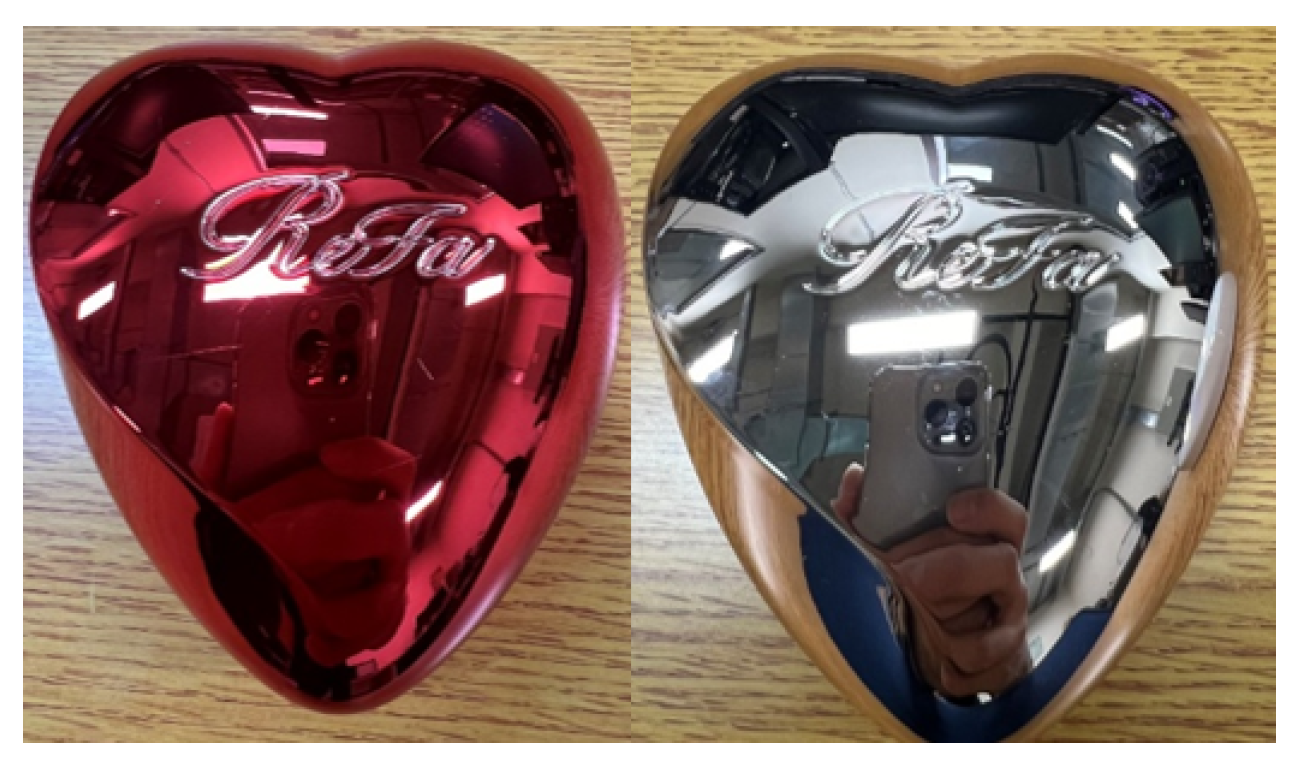
Figure 2.
CNN Layers.
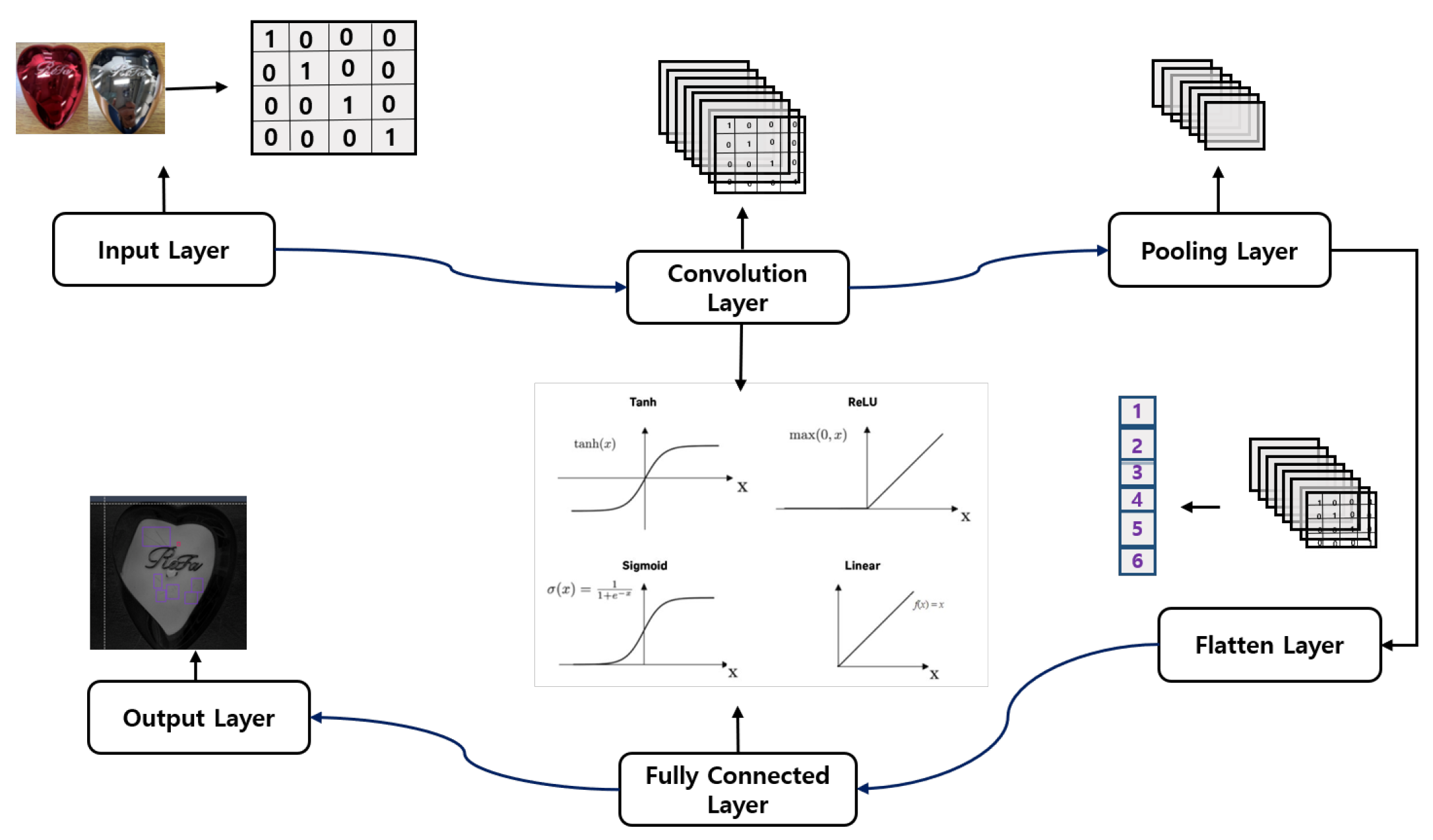
Figure 3.
Proposed System Framework.
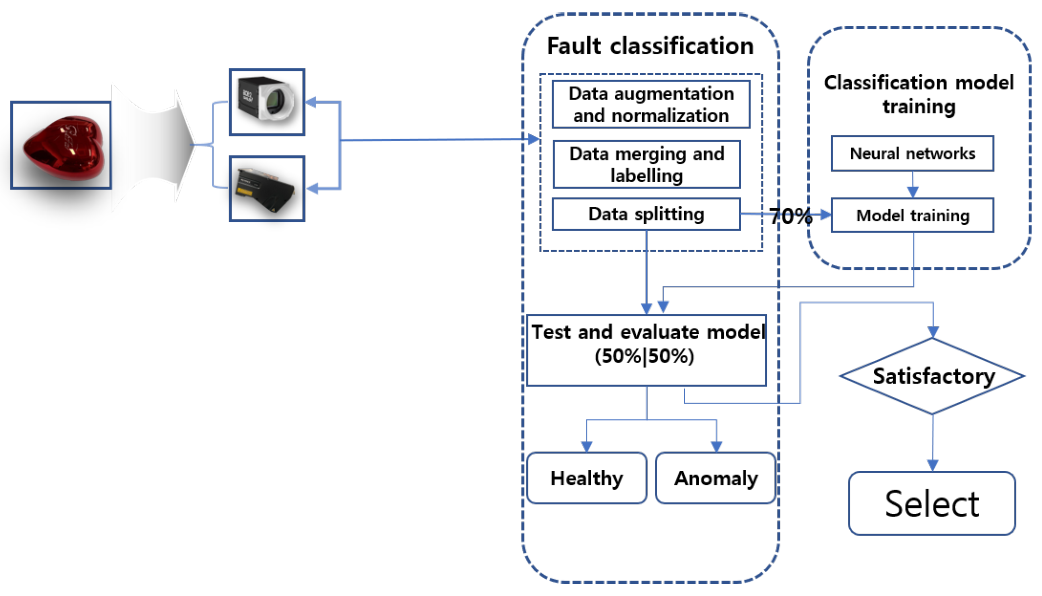
Figure 4.
Basler Vision + Lighting Usage Overview.
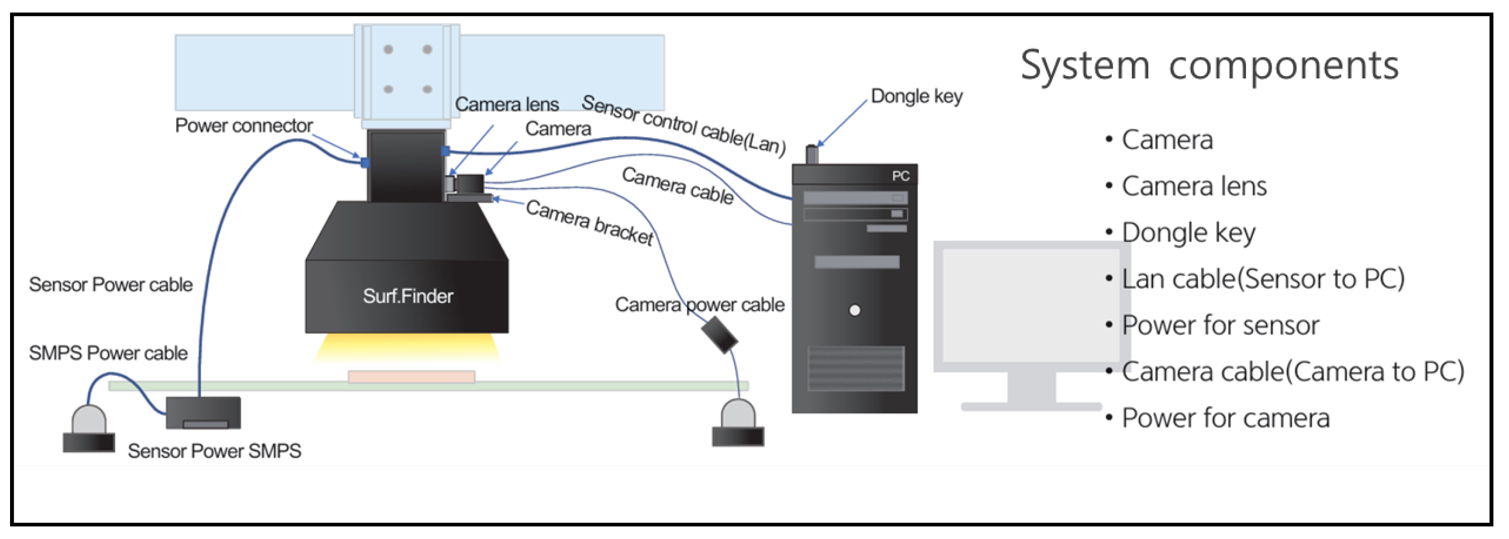
Figure 5.
laser Noise Overview.
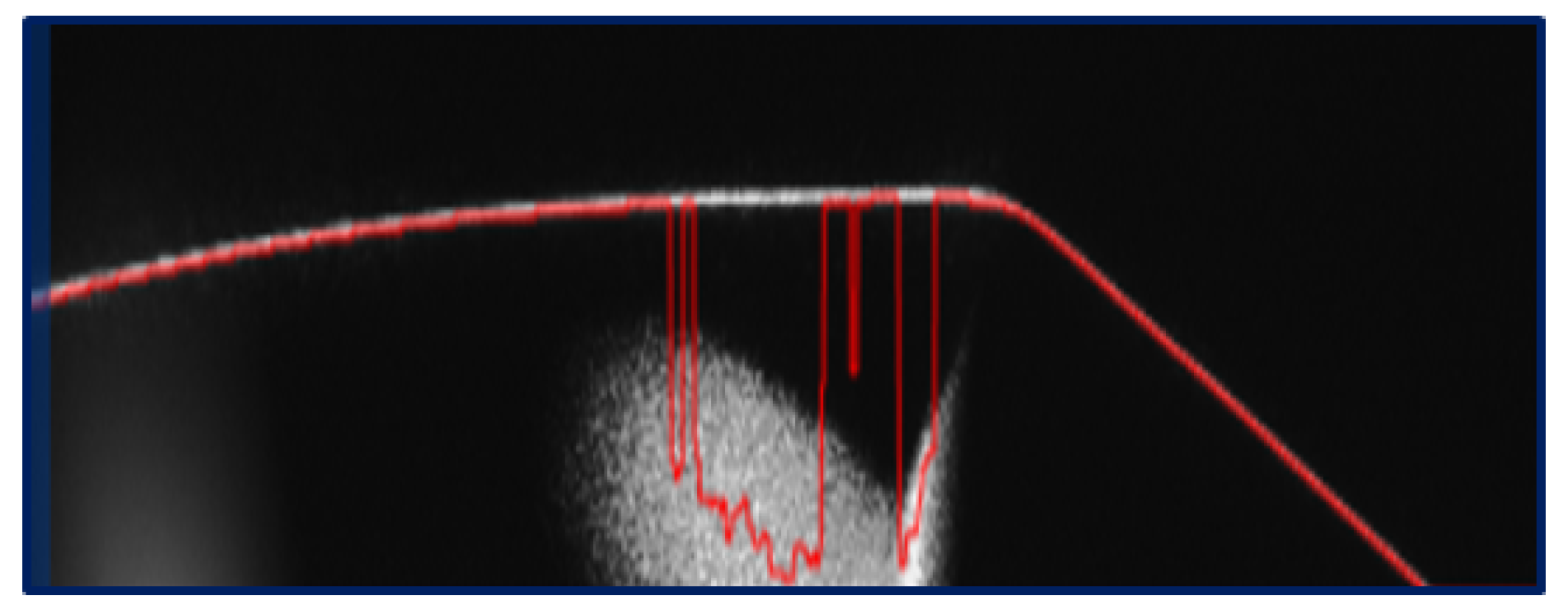
Figure 6.
Robotic Arm
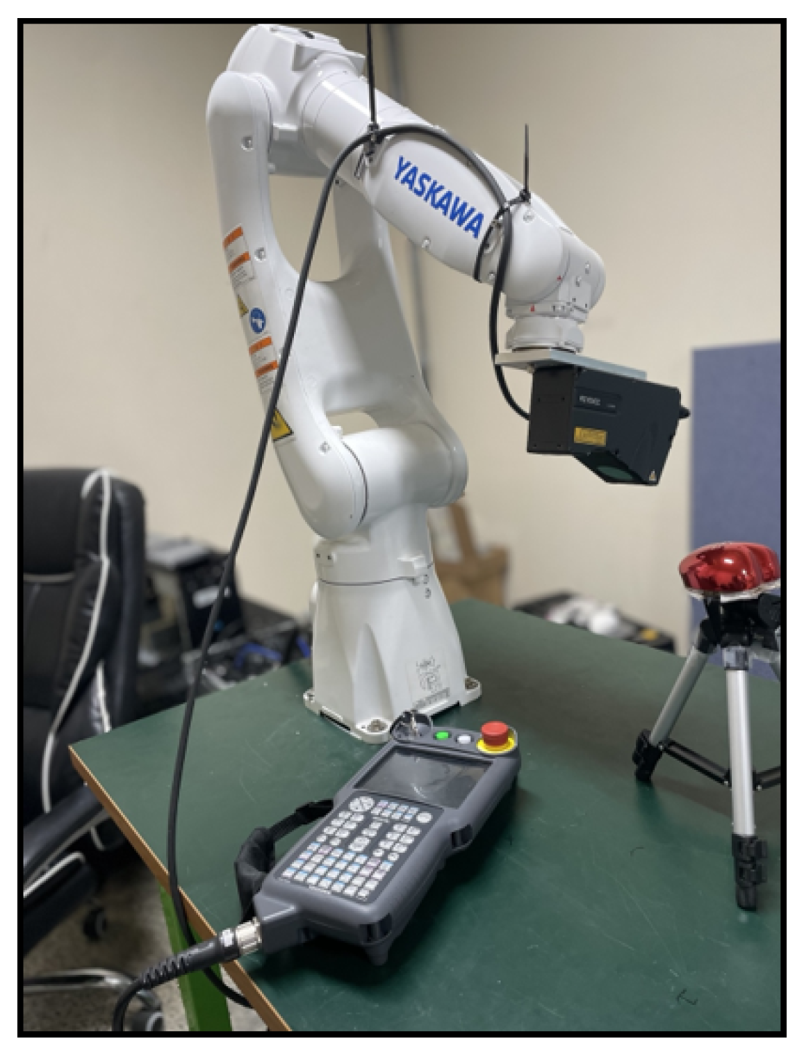
Figure 7.
Coordinates obtained through NC module.
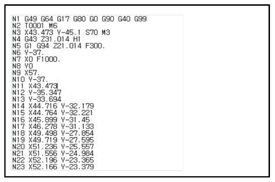
Figure 8.
Laser displacement sensor measurable range based on: (a) data collection speed of 500HZ; (b) data collection speed of 750HZ.
Figure 8.
Laser displacement sensor measurable range based on: (a) data collection speed of 500HZ; (b) data collection speed of 750HZ.
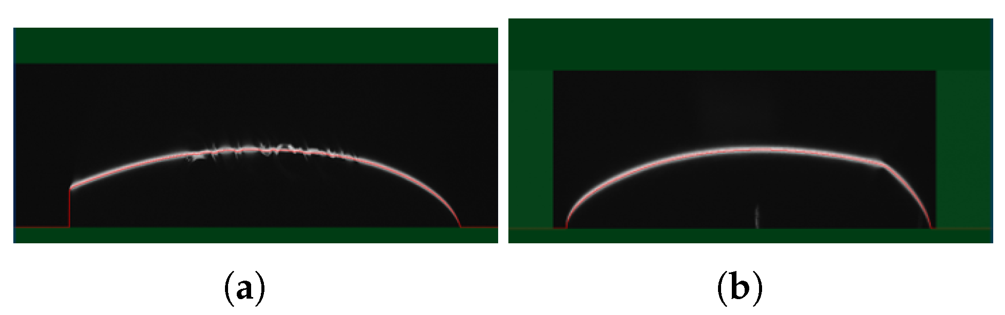
Figure 9.
Image Classes: (a) Healthy class front view; (b) Dent class front view; (c) Dent class front view; d) Healthy class front side view; e) Dent class side view; f) Scratch class front side view.
Figure 9.
Image Classes: (a) Healthy class front view; (b) Dent class front view; (c) Dent class front view; d) Healthy class front side view; e) Dent class side view; f) Scratch class front side view.
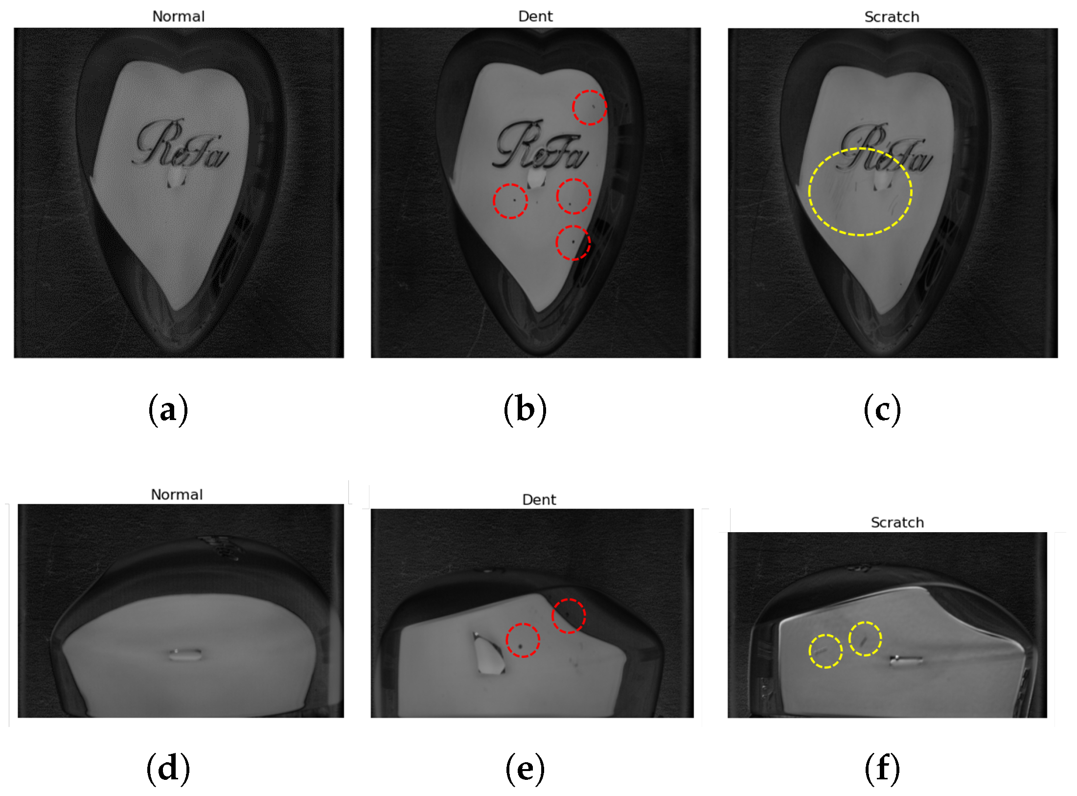
Figure 10.
Accuracy and loss curve: (a) CNN5-128; (b) CNN5-240; (c) CNN6-128; (d) CNN6-240; (e) VGG-16128; (f) VGG-16224; (g) ResNet-50128; (h) ResNet-50224.
Figure 10.
Accuracy and loss curve: (a) CNN5-128; (b) CNN5-240; (c) CNN6-128; (d) CNN6-240; (e) VGG-16128; (f) VGG-16224; (g) ResNet-50128; (h) ResNet-50224.
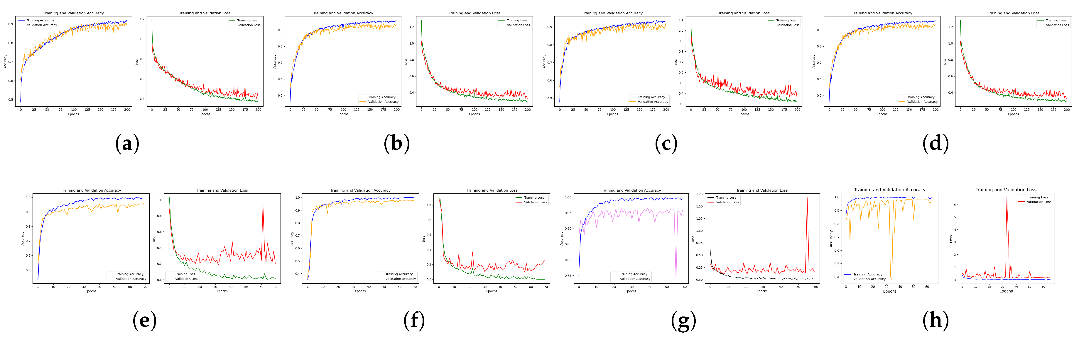
Figure 11.
Confusion matrix: (a) CNN5-128; (b) CNN5-240; (c) CNN6-128; (d) CNN6-240; (e) VGG-16128; (f) VGG-16224; (g) ResNet-50128; (h) ResNet-50224.
Figure 11.
Confusion matrix: (a) CNN5-128; (b) CNN5-240; (c) CNN6-128; (d) CNN6-240; (e) VGG-16128; (f) VGG-16224; (g) ResNet-50128; (h) ResNet-50224.
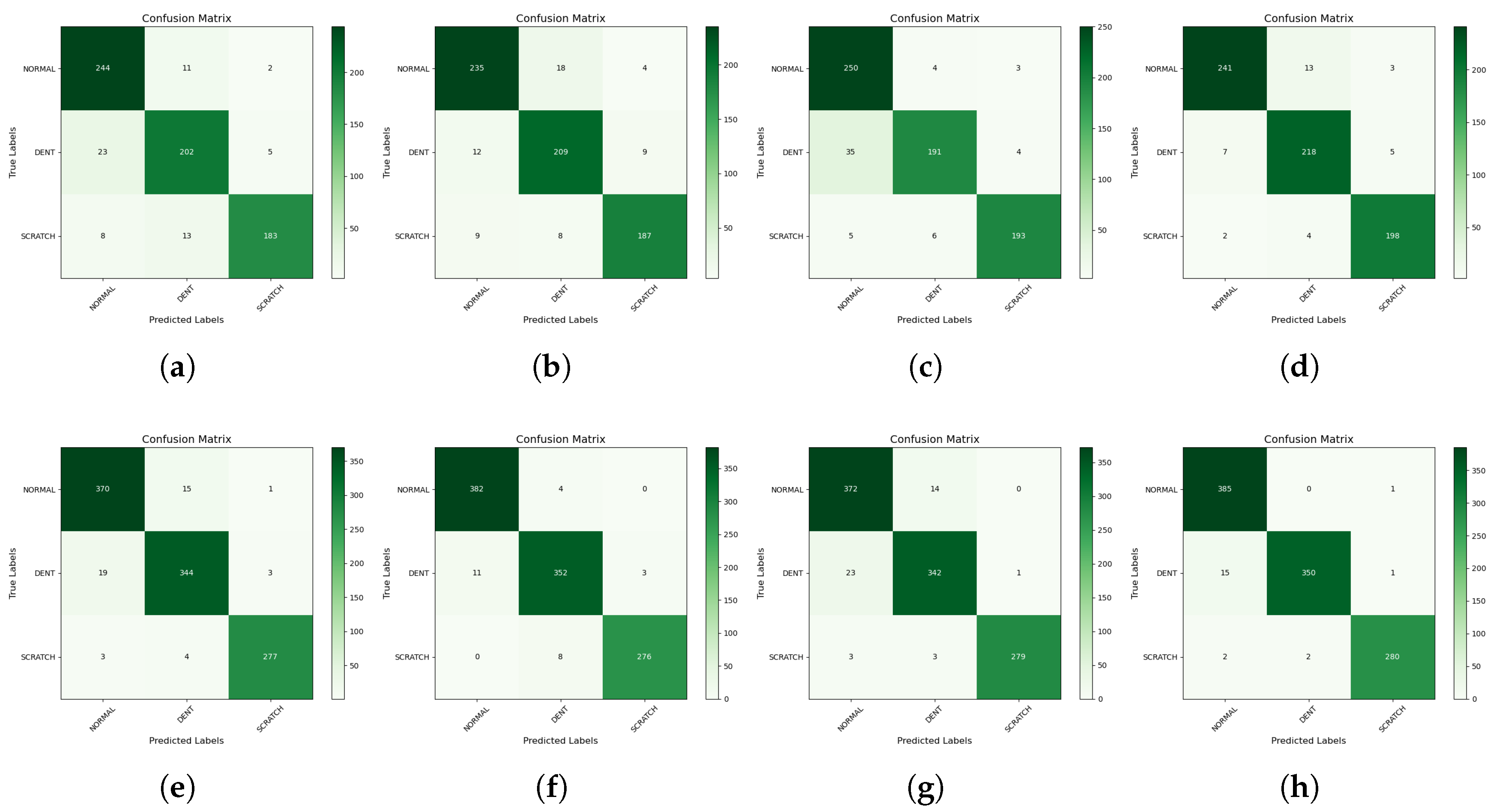
Figure 12.
(a) Model total training time; (b) Model average training step for one Image data; (c) Accuracy.
Figure 12.
(a) Model total training time; (b) Model average training step for one Image data; (c) Accuracy.
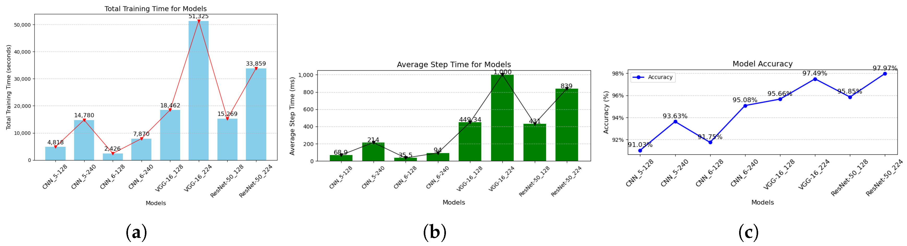

Table 1.
Camera Specification.
| Product Name | Hikvision MV-CA050-20UM |
|---|---|
| Lens | f 35mm |
| Working Distance | 20mm |
| Pixel | 5MP |
| Field of view (FOV) | 91mm x 72mm |
Table 2.
Lighting Specification.
| Product Name | surf.Finder-SF |
|---|---|
| Dimension | 335 x 325 x 330 mm3 |
| (FOV) | 60 x 60 mm2 |
| Weight | 6.9kg |
| Other Accessories | Built-in Controller, S/W Package(SDK, Viewer), Lan cable, SMPS, Dongle key |
Table 3.
Laser Displacement Specification.
| Product Name | LJX-8080 |
|---|---|
| Dimension | 73mm (±20.5mm |
| (FOV) | 60 x 60 mm2 |
| Weight | 6.9kg |
| Other Accessories | Built-in Controller, S/W Package(SDK, Viewer), Lan cable, SMPS, Dongle key |
Table 4.
Measurement Results for Shooting from the Side.
| Number of inspections | Number of coordinates moved | Time (secs) | Inspection speed (mm/s) |
|---|---|---|---|
| 1 | 22 | 21.2 | 11.5 |
| 2 | 23 | 20.8 | 11.5 |
| 3 | 23 | 23.4 | 11.5 |
| 4 | 24 | 25.1 | 11.5 |
| 5 | 23 | 24.2 | 11.5 |
| 6 | 23 | 25.1 | 11.5 |
| 7 | 23 | 23.1 | 11.5 |
| 8 | 23 | 22.9 | 11.5 |
| 9 | 23 | 22.9 | 11.5 |
| 10 | 23 | 26.0 | 11.5 |
Table 5.
Selected Path Information when shooting from the side.
| Number of coordinates moved | Measurement time (secs) | Inspection speed (mm/s) |
|---|---|---|
| 23 | 18.2 | 11.5 |
Table 6.
Selected Path Information While Shooting from the Side.
| Number of coordinates moved | Measurement time (secs) | Inspection speed (mm/s) |
|---|---|---|
| 23 | 14.6 | 13.2 |
Table 7.
Architectures of the Custom CNN Models.
| Model name | Number of Conv layers/stride | Kernel sizes/learning rate | Pooling layer/size | Activation functions | Fully connected layers/dropout | Image dimension | Batch size/Epochs |
|---|---|---|---|---|---|---|---|
| CNN5-128 | 3/1 | 3 x 3/0.001 | 3/2 x 2 | Relu/Softmax | 2/0.1 | 128 x 128 | 16/200 |
| CNN5-240 | 3/1 | 3 x 3/0.001 | 3/2 x 2 | Relu/Softmax | 2/0.1 | 240 x 240 | 16/200 |
| CNN6-128 | 4/1 | 3 x 3/0.001 | 3/2 x 2 | Relu/Softmax | 2/0.1 | 128 x 128 | 16/200 |
| CNN6-240 | 4/1 | 3 x 3/0.001 | 3/2 x 2 | Relu/Softmax | 2/0.1 | 240 x 240 | 16/200 |
Table 8.
Summary of the Modified VGG-16 and ResNet-50 Architecture Employed in the Study.
| Model name | Pre-trained VGG-16 Model | Image Dimension | Dense layer | Dropout Rate | Output Layer | Optimizer/ learning rate |
|---|---|---|---|---|---|---|
| VGG-16128 | ImageNet weights | 128 x 128 | 256, ReLU | 0.2 | Softmax | Adam/0.0001 |
| VGG-16224 | ImageNet weights | 224 x 224 | 256, ReLU | 0.2 | Softmax | Adam/0.0001 |
| ResNet-50128 | ImageNet weights | 128 x 128 | 256, ReLU | 0.2 | Softmax | Adam/0.0001 |
| ResNet-50224 | ImageNet weights | 224 x 224 | 256, ReLU | 0.2 | Softmax | Adam/0.0001 |
Table 9.
performance Evaluation Summary.
| Model | Test accuracy | Test loss | Precision | Recall | F1 Score | Specificity | mAP |
|---|---|---|---|---|---|---|---|
| CNN5-128 | 91.03 | 0.4064 | 91.47 | 90.82 | 91.07 | 95.30 | 0.9697 |
| CNN5-240 | 93.63 | 0.3651 | 91.41 | 91.33 | 91.36 | 95.62 | 0.9723 |
| CNN6-128 | 91.75 | 0.3459 | 92.58 | 91.64 | 91.86 | 95.72 | 0.9795 |
| CNN6-240 | 95.08 | 0.2753 | 95.09 | 95.21 | 95.14 | 97.53 | 0.9878 |
| VGG-16128 | 95.66 | 0.1981 | 95.91 | 95.79 | 95.85 | 97.75 | 0.9906 |
| VGG-16224 | 97.49 | 0.1911 | 97.61 | 97.61 | 97.52 | 98.71 | 0.9963 |
| ResNet-50128 | 95.85 | 0.2073 | 96.21 | 96.21 | 96.12 | 97.83 | 0.9869 |
| ResNet-50224 | 97.97 | 0.1030 | 98.16 | 97.99 | 98.05 | 97.78 | 0.9942 |
Disclaimer/Publisher’s Note: The statements, opinions and data contained in all publications are solely those of the individual author(s) and contributor(s) and not of MDPI and/or the editor(s). MDPI and/or the editor(s) disclaim responsibility for any injury to people or property resulting from any ideas, methods, instructions or products referred to in the content. |
© 2025 by the authors. Licensee MDPI, Basel, Switzerland. This article is an open access article distributed under the terms and conditions of the Creative Commons Attribution (CC BY) license (http://creativecommons.org/licenses/by/4.0/).
Copyright: This open access article is published under a Creative Commons CC BY 4.0 license, which permit the free download, distribution, and reuse, provided that the author and preprint are cited in any reuse.


