
Submitted:
17 March 2025
Posted:
17 March 2025
You are already at the latest version
Abstract
Precise forest inventory is the key to sustainable forest management. LiDAR technology is applied to tree attribute extraction widely. Therefore, this study compared DBH and tree height derived from Handheld Mobile Laser Scanning (HMLS), Airborne Laser Scanning (ALS) and Integrated ALS and HMLS, and determined the applicability of integrating HMLS and ALS scanning methods to estimate individual tree attributes Diameter at Breast Height (DBH) and tree height in pine forests of South Korea. There were strong correlations for DBH at individual tree level (r > 0.95; p < 0.001). HMLS and Integrated ALS˗HMLS achieved high accuracy for DBH estimations, showing Root Mean Squared Error (RMSE) of 1.46 cm (rRMSE 3.7%) and 1.38 cm (rRMSE 3.5%), respectively. In contrast, tree height obtained from HMLS was lower than expected, showing an RMSE of 2.85 m (12.74%) along with a bias of −2.34 m. ALS data enhanced the precision of tree height estimations, achieving a root mean square error (RMSE) of 1.81 m and a bias of -1.24 m. However, integrating ALS and HMLS data resulted in the most precise of the tree height estimations with RMSEs reaching 1.43 m and bias of ˗0.3 m. Integrated ALS and HMLS and its advantages is a beneficial solution for accurate forest inventory which in turn supports forest management and planning.
Keywords:
airborne laser scanning
; handheld mobile laser scanning
; point cloud density
; point cloud registration
; forest inventory
1. Introduction
Forest inventories play a critical role in sustainable forest management and various ecosystem services [1,2]. Traditional field surveys measure tree location, species, DBH, and tree height [3,4,5,6,7,8]; however, parameters such as crown diameter, crown length are not often considered [9]. Therefore, advanced remote sensing techniques are essential for assessing the quality and quantity of forest resources, encompassing factors such as stand structure, composition, and productivity [2].
The introduction of light Detection and Ranging (LiDAR) technology has opened a new era in the forestry field and has been applied to forestry investigation since the early 1980s [3,10,11,12]. Its distinctive features provide tremendous benefits that measure the biological of trees directly through 3D point clouds with high accuracy even at individual tree levels that cannot be obtained by traditional methods [3]. These technologies have the potential to enhance productivity in forest inventory by substituting traditional manual methods of measuring tree characteristics with more automated processes [4,13,14]. In addition, LiDAR mapping proves to be particularly advantageous when a project necessitates precise elevation information for densely vegetated regions, expansive terrains, or locations that are hard to reach or pose safety hazards for ground access [15]. According to Cheng et. al. (2018), LiDAR technology can be categorized into three main types: space-borne LiDAR, which encompasses systems like Unmanned Aerial Vehicle (UAV) LiDAR and airborne laser scanning (ALS); ground-based LiDAR, which includes Terrestrial Laser Scanning (TLS); and vehicle-mounted LiDAR, featuring options such as Handheld Mobile Laser Scanning (HMLS) and Backpack Mobile Laser Scanning (BMLS) [16].
Airborne Laser Scanning (ALS) ALS is a technology that combines a laser scanning device with a global navigation satellite system (GNSS) or an inertial measurement unit (IMU) to achieve accurate positioning and orientation [17]. A significant benefit of ALS is its ability to assess the height of tree canopies and the tops of trees from an aerial perspective on a broad scale [17,18,19]. On the other hand, numerous studies stated that a significant limitation of using ALS in operations is its incompetency to capture complicated structures beneath the canopy [20,21,22,23]. After collecting data using ALS, one of the most common methods for estimating tree height is through the creation of a Canopy Height Model (CHM) that yields a raster dataset where each pixel value corresponds to the height of the vegetation at that location [24,25]. CHM was calculated by taking the difference between the ground elevation, represented by the Digital Elevation Model (DEM), and the elevation of the vegetation canopy, indicated by the Digital Surface Model (DSM) [26,27]. Algorithms like watershed segmentation or local maxima detection are used to identify individual trees within the CHM [22]. Therefore, CHM method was considered a feasible approach for estimating tree heights [1].
Over the past several decades, Terrestrial Laser Scanning (TLS) has been utilized in the field of forestry [28]. TLS concluded ground˗based laser scanning and handheld mobile laser scanning (HMLS) conducted by an operator to gather a highly detailed point cloud in a dynamic way [17]. Since HMLS can capture the finer detail beneath the canopy, besides DBH and height, it also permits the estimation of additional inventory parameters (e.g., crown diameter, stem straightness, foliage biomass) [4,29]. However, HMLS also has challenges when identifying treetops in high and thick canopies or dense understory vegetation [1,9,17]. The heights of trees obtained from HMLS point cloud data frequently show lower than those measured in the field, primarily because of the overlapping canopies of the individual trees [4,10,14,30,31].
Handheld and airborne LiDAR technologies both characterize stand structure through point cloud data. However, while handheld LiDAR examines the canopy from a bottom-up approach, airborne LiDAR systems capture a top-down view of the canopy [2,5]. Because items that are closer to the device usually produce a recognizable return, point clouds collected through airborne laser scanning reveal the upper sections of the canopy, whereas those gathered via handheld laser scanning highlight the lower portions of the tree crowns [2,21]. The integration of HMLS and ALS can be utilized to simulate the structure beneath the canopy as well as the upper canopy. This approach may eventually facilitate an indirect acquisition of the entire canopy structure through airborne LiDAR data collected throughout the landscape [21,32]. Therefore, this paper aimed to compare DHB and tree height obtained by HMLS, ALS and integrated ALS˗HMLS using field surveys as a benchmark in pine forest of Pocheon-si, Republic of Korea. Specifically, we highlighted the advantages of combining ALS and HMLS in forest attributes extraction compared to applying a single approach.
2. Materials and Methods
2.1. Study Area
The study area, which has a coverage of 1.6 ha, is coniferous planted Pinus koraiensis forests in Pocheon-si, Gyeonggi˗do, Republic of Korea (latitude 37°45’58.58”N; longitude 127°10’36.01”E) (Figure 1). The annual precipitation is about 1272.4 mm with a mean temperature of 11.2°C, highest temperature of 17.6°C and lowest temperature of 5.5°C (2011~2020) (Meteorological data open portal, Korea (kma.go.kr). Its topography is relatively gentle, with elevation varying from 154 m to 190 m above sea level.
2.2. Data Collection
The workflow presented in Figure 2 shows the methodology used in this study.
2.2.1. Field Measurement (FM)
Field measurements were conducted from 28 to 29 May 2024, primarily following the forest sampling methodology outlined in Practical Forest Measurement and Survey by the National Institute of Forest Science, South Korea [33]. First, three plots (20m x 20m) were established in the upper, central, and lower sections of the research area. Within these plots, only Pinus koraiensis was selected as the dominant species for measurement purposes. The herbaceous and shrub were regarded as the understory layer. Tree DBH was measured at 1.20 m above ground using a fiberglass diameter tape (SL05001, Shinil Science Co., Ltd., Republic of Korea). Tree height was calculated using Vertex IV (Haglöf Sweden AB, Långsele, Sweden). All measured trees were marked with labels. Then, collected data including tree locations were recorded in inventory form presented by NIFS.

Table 1.
Description of tree attributes from field measurement in three plots. The standard deviation for the sample is indicated within parentheses.
Table 1.
Description of tree attributes from field measurement in three plots. The standard deviation for the sample is indicated within parentheses.
| Attributes | Plot 1 | Plot 2 | Plot 3 |
|---|---|---|---|
| Min DBH (cm) | 29.2 | 23.1 | 36.5 |
| Max DBH (cm) | 46.8 | 57.9 | 62.8 |
| Mean DBH (cm) | 36.88 (4.63) | 39.14 (8.03) | 43.01(7.37) |
| Min tree height (m) | 16.2 | 20.3 | 18.0 |
| Max tree height (m) | 23.8 | 25.4 | 25.9 |
| Mean tree height (m) | 21.15 (2.35) | 22.66 (2.31) | 22.09 (1.89) |
| Plot size (m2) | 400 | 400 | 400 |
| No. of trees (#) | 14 | 17 | 11 |
| Tree density (tree/ha) | 350 | 425 | 275 |
| Basal area (m2) | 0.61 | 0.83 | 0.65 |
2.2.2. Handheld Mobile Laser Scanning (HMLS)
Point cloud data scanning was conducted from 28 to 29 May 2024 in the field using a handheld ZEB Horizon scanner (GeoSLAM Ltd., Nottingham, United Kingdom) (Table 2) carried by forest surveyor (Figure 3A). The sensor emits continuous laser beams that scatter as near-infrared rays with a wavelength of 905nm [34]. The surrounding objects respond to this by reflecting the emitted pulses. Then, the sensor calculates the distance of objects and captures their angles in a two-dimensional (2-D) format. Simultaneously, a SLAM algorithm integrates the 2-D profiles with data from the IMU to create 3-D point clouds without using GNSS receiver [28,34].
Before HMLS data acquisition, the plot center and four corners of the plots were marked by four poles (0.7m length) to help the data analyst quickly identify the plot position and plot boundary when clipping the sample plot on a 3˗D point cloud (Figure 3A). In addition, two cars were placed on the border of the study area under an open˗spaced area to use as identified objects for data registration of handheld and airborne LiDAR point clouds. A parralel walking cross plot at a consistent distance was performed to achive the maximum number of loops and the loop is completed by returning to the initial position (Figure 3B). The loop is important for the SLAM algorithm as it allows for resurvey of known positions [23,30,34]. This primary approach used with GeoSLAM mobile scanners help minimize drift error and obtain highest density of points [23]. Plots were scanned slowly at a speed of 1m/sec with stable movement to guarantee both point cloud quality data and its coverage [34].
2.2.3. Airborne Laser Scanning (ALS)
Airborne point cloud data was acquired on May 29 using a LiDAR scanner (YellowScan, France) mounted in a Matrice 300 RTK drone (DJI Enterprise, China) (Figure 3C). The UAV flight measurement covers about 1.5 ha. The flight was conducted two times with different attitude (100m and 70m above ground level) with side overlaps of 80 %. Base station and seven Ground Control Points (GCPs) were distributed within the area to receive satellite positioning data and send it to a GNSS receiver (Figure 3D). Precise coordinates were added to point cloud data using POSPAC, then a complete point cloud was created using CloudStation software (YellowScan, France). For reference use purposes, an RGB image was also acquired using a DJI Phantom 4 Pro quadcopter UAV (DJI Enterprise, China), then an orthophoto of the study site was obtained using UAV Applications Master version 13.2.3 (Trimble, Stuttgart, Germany).
2.3. Point Cloud Data Analyses
2.3.1. HMLS
HMLS point clouds were processed by LiDAR360 software version 5.4 (GreenValley International, Berkeley, CA, USA). The data set was filtered using the Outlier Removal tool in LiDAR360 to remove noise points caused by wind and multipath effects. Smooth Points based on the neighboring points make the point cloud look more consistent. Normalization was done to eliminate the effect of terrain elevation on LiDAR height. Then point cloud was sliced at 1.2m in 2D environment to manually measure the DBH of individual trees and use them as seed points for point cloud segmentation (Figure 4A, B). Visual inspection was subsequently conducted to correct the possible segmentation mistakes found in the point cloud of each individual tree (Figure 4C).
2.3.2. ALS
For ALS point cloud, Remove Outliers and Smooth Points were also applied. Then, a Canopy Height Model (CHM) was created by subtracting DSM from DEM according to Douss et. al. (2022) [26]. First, a classification algorithm that operates automatically was utilized to separate the point cloud into ground points and vegetation points. Ground points were interpolated into DEM using an Inverse Distance Weighting (IDW) interpolation method (Figure 5A). For the DSM, a similar grid˗based interpolation approach was applied to generate the surface capturing the vegetation canopy (Figure 5B). The difference between the DSM and DEM was calculated to derive the Canopy Height Model (CHM), which provides insight into vegetation height and structure (Figure 5C). The pixel size was 10 cm × 10 cm for all raster data.
2.3.3. ALS and HMLS Registration
ALS and HMLS point clouds were registered in Trimble RealWorks Advanced˗Plant® 11.0 version (Trimble, Stuttgart, Germany) with the cloud˗based registration function using artificial objects (e.g., cars) to register two˗point clouds. Point cloud from ALS, which contains local coordinate systems served as references and point cloud from HMLS, was moving cloud. As a result, the achieved accuracy was 2 cm (Figure 6).
2.3.4. Density Assessment
To calculate the point density of ground and vegetation subsets from a point cloud, the following methodology was employed. First, the LiDAR point cloud data was preprocessed to ensure accuracy and uniformity, including noise removal and coordinate system verification. Next, the data was classified into ground and vegetation points using an automated classification algorithm in LiDAR360, which assigns points to specific categories based on their height and spatial characteristics. Once the classification was complete, the dataset was divided into two subsets: ground points and vegetation points. Each subset was processed independently to compute point density. A grid˗based approach was utilized, wherein the region of interest was divided into uniform grid cells of a predefined size (1m × 1m). For each subset, the total number of points falling within each grid cell was counted, and the density was calculated as the number of points per unit area (points/m2).
2.4. Accuracy Assessment
Shapiro˗Wilk test was used to determine normal distribution of DBH and tree height. Then, Pearson’s correlation analysis was applied to normally distributed data while data without normality were subjected to Spearman’s correlation analyses. Besides, paired samples t-test was utilized to assess whether there were any notable differences in tree diameter at breast height (DBH) and tree height as measured by three different methods. The accuracy assessment was additionally conducted using Root Mean Squared Error (RMSE), relative RMSE (rRMSE), bias, relative bias (rBias), Mean Absolute Error (MAE), using the field measurements as the reference data, represented by equations from (1) to (5) [6]. Consequently, any potential linear relationships were examined visually. All statistical analyses were conducted using SPSS software, adhering to a significance level of less than 5%.
where is the DBH value extracted from HMLS, is the DBH measured in the field, n is the number of trees in each plot, is the error term, is the mean of field survey, i is the sample index.
3. Results
3.1. Point Cloud Density
Point cloud density (points/m2) for both ground and vegetation across three plots, measured from ALS, HMLS, and Integrated ALS˗HMLS were shown in Table 3.
Ground points extracted from point clouds are important for DEM generation and other analyses. Regarding ground point density, the data indicates that ALS consistently recorded the lowest density (between 13 and 16 points/m2) among all plots HMLS. On the other hand, HMLS revealed a significant increase in ground point density, with measurements between 1,157 and 3,389 points/m2. The combination of ALS and HMLS resulted in a minor enhancement producing values ranging from 1,167 to 3,393 points/m2. However, a very low density in ground point was shown in ALS (avg. 11 points/m2), which demonstrates limited capability of ALS in capturing ground˗level details. Compared to ALS, HMLS exhibits a much higher resolution of ground surfaces (avg. 2338 points/m2). This underscores its superior capability in resolving vegetation structures. The integration offers moderate improvements over HMLS, suggesting a complementary effect of ALS in refining the results.
In terms of vegetation, ALS presents the lowest point densities, which lie between 2,398 and 2,793 points/m2, reflecting its limited capacity to capture intricate details of vegetation. HMLS, however, experiences a notable escalation, with densities recorded between 21,315 and 26,727 points/m2. The integrated ALS˗HMLS approach further boosts vegetation point densities, reaching the highest values across all plots, between 23,710 and 29,129 points/m2. HMLS significantly outperforms ALS in capturing both ground and vegetation densities, demonstrating its efficacy for detailed point cloud generation. The Integrated ALS˗HMLS method provides incremental improvements over HMLS, emphasizing the advantage of combining the strengths of both ALS and HMLS methods.
3.2. Diameter at Breast Height (DBH)
Table 4 indicates average DBH values estimated from HMLS and Integrated ALS˗HMLS approaches and their test results. As seen in Table 4, the two approaches (HMLS and Integrated ALS˗HMLS) showed highly positive correlated DBH measurements, with statistically significant correlations in all cases (r > 0.93, p < 0.001). The normality test showed DBH values were normally distributed (p > 0.05) in plot 1 and plot 2 but plot 3 and the overall dataset (p < 0.05).
Figure 7 displays scatterplots comparing the diameter at breast height (DBH) measurements obtained from field measurements (FM) with HMLS and Integrated ALS˗HMLS remote sensing approaches. Figure 7 demonstrates that both HMLS and Integrated ALS˗HMLS approaches yield DBH measurements strongly correlated with field measurements. Regression equations indicate that both remote sensing methods provide accurate and reliable estimations of DBH, with minor differences in slope and intercept adjustments. These results validate the effectiveness of the remote sensing approaches for DBH measurement.
Table 5 presents an evaluation of the accuracies of the two methods. Plot 3 achieved the most precise estimation of DBH, utilizing the HMLS method, with the lowest values for RMSE (1.10 cm) and MAE (0.91 cm). In contrast, Plot 1 reflects a moderate level of accuracy; however, it reports a slightly elevated RMSE of 1.54 cm and a bias of ˗0.66 cm. Plot 2 exhibits a higher RMSE of 1.59 cm and a bias of ˗1.28 cm, suggesting it has less alignment with field measurements. All estimations displayed a negative bias, indicating that the HMLS method’s DBH measurements were smaller than those obtained through manual field measurements.
3.3. Height
Table 6 reveals that the Integrated ALS˗HMLS method consistently yields the highest average tree height estimates across all plots, reaching an overall mean of 23.03 m, followed by ALS at 21.09 m and HMLS at 19.99 m. Although ALS and Integrated ALS˗HMLS demonstrate moderate correlations with field measurements, particularly noticeable in Plot 2 and 3, the correlations observed for HMLS are generally weaker. The results of the normality test indicate that HMLS approach in Plot 1 and the complete dataset do not conform to normal distribution. These results imply that Integrated ALS˗HMLS and ALS are more dependable and consistent in estimating tree heights when compared to HMLS.
The tree height estimation from HMLS and the Integrated HMLS and ALS are compared to reference field measurement data in Figure 8. The chart displayed the precision metrics for tree height estimation across three different plots utilizing HMLS (Handheld Mobile Laser Scanning), Integrated ALS˗HMLS, and ALS (Airborne Laser Scanning) in comparison to the reference data.
Under the HMLS methodology, tree height was significantly underestimated, resulting in an RMSE of 5.13m, an MAE of 4.75m as displayed in Table 7. Conversely, when HMLS was integrated with ALS, there was an enhancement in bias and other precision indicators, including an RMSE of 1.56 m and an MAE of 1.25m. At the level of individual plots, HMLS exhibited the highest RMSE, varying from 2.55 to 3.13cm, with a bias range of 2.14 to 2.57cm and MAE values lying between 2.26 and 2.57cm, closely followed by ALS. In stark contrast, the combined ALS˗HMLS approach produced the most advantageous outcomes, achieving the lowest RMSE of 1.66cm for both bias and MAE. Overall, the Integrated ALS˗HMLS method achieved the best accuracy, marked by a minimum RMSE of 1.43cm, a relative root mean square error of 6.41%, a bias of ˗0.30cm, and an MAE of 1.10 cm. While ALS demonstrated moderate performance, it recorded higher error levels with an RMSE of 1.81cm and a bias of ˗1.24cm compared to the Integrated ALS˗HMLS approach. Meanwhile, HMLS showed the highest levels of error and an underestimation, reaching a peak RMSE of 2.85cm, accompanied by a bias of ˗2.30cm. The negative bias implies that the estimates provided by all three methods fell short of the actual reference values.
4. Discussion
4.1. Point Cloud Density
Point cloud density is one of the most important parameters in LiDAR data analyses [35]. In this study, the differences in point cloud densities among ALS, HMLS, and integration of ALS and HMLS were determined to demonstrate the strengths and limitations of each approach. According to Balsa et. al. (2012), ALS consistently records the lowest point densities, particularly for ground points, due to its airborne scanning characteristics [35]. With a larger footprint and lower resolution at ground level, ALS struggles to capture fine scale details, leading to sparse point distributions [36,37]. In addition, this limitation impacts its ability to extract precise terrain features, which are essential for applications such as digital elevation model (DEM) generation and forest structure analysis [38].
In contrast, HMLS exhibits significantly higher densities for both ground and vegetation points because of the close range and high resolution scanning capabilities of the technology [28]. By capturing a higher level of detail, HMLS enhances the accuracy of point cloud˗based analyses, particularly in complex forest environments where high density data is crucial for structural assessments [39]. The substantial increase in ground point density compared to ALS indicates that HMLS is more effective in capturing detailed terrain features, making it a valuable tool for applications requiring fine resolution point clouds [40]. Similarly, for vegetation, the higher density from HMLS provides a more comprehensive representation of tree trunks, which is critical for biomass estimation and ecological modelling [41].
The integration of ALS and HMLS in this study offers an optimal balance between broad coverage and high detail capture, resulting in improved overall point densities. By leveraging ALS’s capability to cover large areas efficiently and HMLS’s ability to provide detailed local measurements, the integrated approach enhances data completeness, especially in tree height estimation of this study. This approach makes ALS˗HMLS integration the most effective method for capturing both ground and vegetation features, as it mitigates the individual limitations of each technique while maximizing their advantages as approved in study by Lee et. al. (2022) [42]. Consequently, the combined approach holds significant potential for improving forest inventory accuracy, terrain modelling, and vegetation characterization [4,6,10].
4.2. Tree DBH
Study results found that the combination of ALS and HMLS did not enhance the accuracy of DBH estimation. For example, the average DBH calculated from HMLS (38.48 cm) was very similar to that derived from the combined HMLS and ALS approach (38.5 cm). The study further demonstrated that HMLS is a promising approach for assessing tree DBH, achieving a notable accuracy with an RMSE of 1.46 cm (rRMSE=3.7%) across all study plots. Similar findings were reported in previous research that assessed DBH within the range of 1 cm to 3.3 cm in conifer forests in Italy [4], Japan [6] and Scots pine forests in Finland [43]. Outcomes from this study were close to what was found in Yunnan pine forest (RMSE=1.17 cm) in China [30]. Additionally, the mean absolute error was identical for the two approaches (MAE=1.21 cm), indicating that ALS did not contribute in DBH due to its limitations in capture detail beneath canopy. Moreover, the bias values for DBH measurements obtained from HMLS and the integrated ALS-HMLS were approximately equal to 1 and negative, -0.92 cm and -0.9 cm, respectively (Table 5). This finding illustrated that DBH estimated from LiDAR technology in this study was unbiased and smaller than field measurement data. This bias was aligned with earlier studies of Gianneti et. al. (2018) [4] who reported a bias of -0.38 cm using handheld ZEB1 in Mediterranean forest stands, and Bauwens et. al. (2016) [9] who addressed a very small bias of -0.08 cm. As shown in Figure 9, the random positive and negative variances in the DBH predictions displayed a consistent trend near the zero levels, indicating that the calculated DBHs were typically free from bias.
4.3. Tree Height
Tree height measurements using HMLS data in this study resulted in a significant underestimation. Study corresponds with results from Lee et. al. (2022) who compared tree height from integrated ALS and HMLS with ground truth with RMSE of 2 m [42]. Additionally, a similar study conducted in Taebek reported an RMSE of 3.297 m, MAE of 2.303 m and bias of -1.905 m [44]. However, RMSE of HMLS LiDAR in present study was higher than findings from Liu et. al. (2018) who report very small RMSE (0.54m) in tree height using TLS [30]. Primary sources of error in the tree height estimation using HMLS LiDAR technology include tree crown’s top being blocked by itself or neighboring trees, leading to the incorrect identification of tree top during segmentation process. Another study pointed out that inaccuracy in tree height measurement with handheld LiDAR arise from certain parts of a taller adjacent tree’s crown being wrongly identified as the top of the target tree, or mistakes in associating trees during the assessment process [45].
Tree height results from combined ALS˗HMLS were closer to field measurement than those from the HMLS method. This result aligns with previous findings, as airborne LiDAR can improve accuracy of tree height [31]. Besides, Gyawali et. al. (2022) reported a strong correlation between field measurement and airborne LiDAR˗derived heights with an RMSE of 1.44 m and a bias of 0.7 m [46]. Wang et. al. 2019 found a RMSE of 1.6 m and bias of -0.96 m in easy plot of boreal forest in Finalnd [7]. In past studies, the RMSE and bias increase across tree density increase, highlighting the effect of obstructed understory and dense canopy contribute to uncertainties on tree height estimation, associated with the instability of the field measurements [1,47]. This underscores the necessity to improve the crown delineation algorithm to provide dependable outcomes, especially in dense forest environments, especially when the trees were taller than 15 m [7,27,48]. Gianettti et. al. (2018) highlighted the benefits of merging ALS and HMLS, noting a reduction in RMSE from 2.14m to 0.94m and bias move from -4.61 to – 0.3 for both coniferous and broadleaves in Italy [4]. In addition, Sibona et. al. (2017) directly measured felled tree height and compared it to LiDAR scanning [18]. Mean absolute difference was 1.04 m for Scots pine, referring that tree heights estimation by LiDAR scanning was closer to actual tree heights than traditional field-based survey, particularly for tall trees with conical crown shapes. Figure 10 illustrates the random positive and negative fluctuations in estimation of tree height, suggesting that the estimated tree heights from 3 approaches were generally unbiased.
Overall, ALS effectively measures the height of trees, but it is not suitable for assessing DBH and other attributes near ground since it primarily captures tree tops and above canopy. On the other hand, HMLS can estimate both DBH and tree height, however, it often results in underestimations because of thick understory vegetation. Integration of ALS and HMLS is considered the most optimal approach for forest inventory purpose (Table 8) as this method maximizes the advantages of each ALS and HMLS methods while reducing challenges associated with their application [4].
Although many previous studies utilize field-based surveys as a standard for assessing LiDAR estimations, the tree height accuracy is not confident due to equipment malfunction, the expertise and experience of the surveyors, steep slopes, and dense tree populations that complicate the identification of tree tops [18]. Additional significant sources of error in DBH also come from measurement inaccuracies and noise, areas with insufficient point density, and branches and trunks that are not circular [43]. The sample plot is square and its edges can lead to inaccuracies in actual tree top identification because of the closed-boundary configuration. Consequently, additional studies need to incorporate more precise methods for measuring trees in the field to achieve optimal accuracy in tree height calculation in conjunction with LIDAR estimations.
5. Conclusions
This study examined the accuracy of each approach by evaluating point cloud density and found that the combination of ALS and HMLS produces the highest density point clouds, which provide more detailed information about forest stands. High point cloud density enhanced more precise measurements of Diameter at Breast Height (DBH) and tree height, thereby improving the overall accuracy and reliability of forest inventory data obtained from Integrated ALS and HMLS approach. The results of this study also supported that HMLS offers an accurate and non˗destructive estimation of DBH compared to field survey. In contrast, ALS is a good approach to measure tree height thanks to its ability to capture tree tops and detail canopy but it is limited in capturing detail under canopy, specifically tree DBH. Therefore, as a forthcoming LiDAR application, the combined ALS and HMLS method could transform forest inventory methods, overcoming the challenges of traditional ground˗based surveys and allowing for quicker and more expandable forest evaluations and contributing to sustainable management and preservation efforts.
Author Contributions
Conceptualization, M.J.K., H.S.B. and L.T.N.T.; methodology, M.J.K., H.S.B. and L.T.N.T.; software, L.T.N.T. and H.S.B.; formal analysis, L.T.N.T.; investigation, L.T.N.T. and H.S.B.; data curation, L.T.N.T.; writing—original draft preparation, L.T.N.T.; writing—review and editing, L.T.N.T., B.B.P., S.M.C.; visualization, L.T.N.T.; supervision, M.J.K.; project administration, H.S.B.; funding acquisition, M.J.K., H.S.B. All authors have read and agreed to the published version of the manuscript.
Funding
This study was carried out with the support of Development of K-Forest Management Model based on Stand Characteristics for Improvement of Ecosystem Service (grant number RS-2022-KF002152) provided by Korea Forest Service (Korea Forestry Promotion Institute).
Conflicts of Interest
The authors declare no conflicts of interest.
Abbreviations
The following abbreviations are used in this manuscript:
| LiDAR | Light Detection and Ranging |
| UAV | Unmanned Aerial Vehicle |
| ALS | Airborne Laser Scanning |
| TLS | Terrestrial Laser Scanning |
| BMLS | Backpack Mobile Laser Scanning |
| HMLS | Handheld Mobile Laser Scanning |
| GNSS | Global Navigation Satellite System |
| IMU | Inertial Measurement Unit |
| CHM | Canopy Height Model |
| DEM | Digital Elevation Model |
| DSM | Digital Surface Model |
| DBH | Diameter at Breast Height |
References
- Hyyppä, E.; Yu, X.; Kaartinen, H.; Hakala, T.; Kukko, A.; Vastaranta, M.; Hyyppä, J. Comparison of Backpack, Handheld, under-Canopy UAV, and above-Canopy UAV Laser Scanning for Field Reference Data Collection in Boreal Forests. Remote Sens (Basel) 2020, 12, 1–31. [Google Scholar] [CrossRef]
- White, J.C.; Coops, N.C.; Wulder, M.A.; Vastaranta, M.; Hilker, T.; Tompalski, P. Remote Sensing Technologies for Enhancing Forest Inventories: A Review. Canadian Journal of Remote Sensing 2016, 42, 619–641. [Google Scholar] [CrossRef]
- Ghimire, S.; Xystrakis, F.; Koutsias, N. Using Terrestrial Laser Scanning to Measure Forest Inventory Parameters in a Mediterranean Coniferous Stand of Western Greece. PFG - Journal of Photogrammetry, Remote Sensing and Geoinformation Science 2017, 85, 213–225. [Google Scholar] [CrossRef]
- Giannetti, F.; Puletti, N.; Quatrini, V.; Travaglini, D.; Bottalico, F.; Corona, P.; Chirici, G. Integrating Terrestrial and Airborne Laser Scanning for the Assessment of Single-Tree Attributes in Mediterranean Forest Stands. Eur J Remote Sens 2018, 51, 795–807. [Google Scholar] [CrossRef]
- Ma, K.; Xiong, Y.; Jiang, F.; Chen, S.; Sun, H. A Novel Vegetation Point Cloud Density Tree-Segmentation Model for Overlapping Crowns Using UAV LiDAR. Remote Sensing 2021, 13, 1442. [Google Scholar] [CrossRef]
- Shimizu, K.; Nishizono, T.; Kitahara, F.; Fukumoto, K.; Saito, H. Integrating Terrestrial Laser Scanning and Unmanned Aerial Vehicle Photogrammetry to Estimate Individual Tree Attributes in Managed Coniferous Forests in Japan. International Journal of Applied Earth Observation and Geoinformation 2022, 106, 102658. [Google Scholar] [CrossRef]
- Wang, Y.; Lehtomäki, M.; Liang, X.; Pyörälä, J.; Kukko, A.; Jaakkola, A.; Liu, J.; Feng, Z.; Chen, R.; Hyyppä, J. Is Field-Measured Tree Height as Reliable as Believed – A Comparison Study of Tree Height Estimates from Field Measurement, Airborne Laser Scanning and Terrestrial Laser Scanning in a Boreal Forest. ISPRS Journal of Photogrammetry and Remote Sensing 2019, 147, 132–145. [Google Scholar] [CrossRef]
- Xie, Y.; Zhang, J.; Chen, X.; Pang, S.; Zeng, H.; Shen, Z. Accuracy Assessment and Error Analysis for Diameter at Breast Height Measurement of Trees Obtained Using a Novel Backpack LiDAR System. For Ecosyst 2020, 7, 1–11. [Google Scholar]
- Bauwens, S.; Bartholomeus, H.; Calders, K.; Lejeune, P.; Hyyppä, J.; Liang, X.; Puttonen, E. Forest Inventory with Terrestrial LiDAR: A Comparison of Static and Hand-Held Mobile Laser Scanning. Forests 2016, 7, 127. [Google Scholar] [CrossRef]
- Bazezew, M.N.; Hussin, Y.A.; Kloosterman, E.H. Integrating Airborne LiDAR and Terrestrial Laser Scanner Forest Parameters for Accurate Above-Ground Biomass/Carbon Estimation in Ayer Hitam Tropical Forest, Malaysia. International Journal of Applied Earth Observation and Geoinformation 2018, 73, 638–652. [Google Scholar] [CrossRef]
- Hauglin, M.; Lien, V.; Næsset, E.; Gobakken, T. Geo-Referencing Forest Field Plots by Co-Registration of Terrestrial and Airborne Laser Scanning Data. Int J Remote Sens 2014, 35, 3135–3149. [Google Scholar] [CrossRef]
- Yang, B.; Zang, Y.; Dong, Z.; Huang, R. An Automated Method to Register Airborne and Terrestrial Laser Scanning Point Clouds. ISPRS Journal of Photogrammetry and Remote Sensing 2015, 109, 62–76. [Google Scholar] [CrossRef]
- Liang, X.; Kankare, V.; Hyyppä, J.; Wang, Y.; Kukko, A.; Haggrén, H.; Yu, X.; Kaartinen, H.; Jaakkola, A.; Guan, F.; Holopainen, M.; Vastaranta, M. Terrestrial Laser Scanning in Forest Inventories. ISPRS Journal of Photogrammetry and Remote Sensing 2016, 115, 63–77. [Google Scholar] [CrossRef]
- Novotny, J.; Navratilova, B.; Albert, J.; Cienciala, E.; Fajmon, L.; Brovkina, O. Comparison of Spruce and Beech Tree Attributes from Field Data, Airborne and Terrestrial Laser Scanning Using Manual and Automatic Methods. Remote Sens Appl 2021, 23, 2352–9385. [Google Scholar] [CrossRef]
- Carson, W.W.; Andersen, H.-E.; Reutebuch, S.E.; Mcgaughey, R.J. LIDAR APPLICATIONS IN FORESTRY-AN OVERVIEW.
- Cheng, L.; Chen, S.; Liu, X.; Xu, H.; Wu, Y.; Li, M.; Chen, Y. Registration of Laser Scanning Point Clouds: A Review. Sensors 2018, 18, 1641. [Google Scholar] [CrossRef] [PubMed]
- Fekry, R.; Yao, W.; Cao, L.; Shen, X. Ground-Based/UAV-LiDAR Data Fusion for Quantitative Structure Modeling and Tree Parameter Retrieval in Subtropical Planted Forest. For Ecosyst 2022, 9, 100065. [Google Scholar] [CrossRef]
- Sibona, E.; Vitali, A.; Meloni, F.; Caffo, L.; Dotta, A.; Lingua, E.; Motta, R.; Garbarino, M. Direct Measurement of Tree Height Provides Different Results on the Assessment of LiDAR Accuracy. Forests 2016, 8, 7. [Google Scholar] [CrossRef]
- Chehreh, B.; Moutinho, A.; Viegas, C. Latest Trends on Tree Classification and Segmentation Using UAV Data—A Review of Agroforestry Applications. Remote Sensing 2023, 15, 2263. [Google Scholar] [CrossRef]
- Choi, H.; Song, Y. Comparing Tree Structures Derived among Airborne, Terrestrial and Mobile LiDAR Systems in Urban Parks. GIsci Remote Sens 2022, 59, 843–860. [Google Scholar] [CrossRef]
- Hilker, T.; van Leeuwen, M.; Coops, N.C.; Wulder, M.A.; Newnham, G.J.; Jupp, D.L.B.; Culvenor, D.S. Comparing Canopy Metrics Derived from Terrestrial and Airborne Laser Scanning in a Douglas-Fir Dominated Forest Stand. Trees - Structure and Function 2010, 24, 819–832. [Google Scholar]
- Yang, J.; Kang, Z.; Cheng, S.; Yang, Z.; Akwensi, P.H. An Individual Tree Segmentation Method Based on Watershed Algorithm and Three-Dimensional Spatial Distribution Analysis from Airborne LiDAR Point Clouds. IEEE J Sel Top Appl Earth Obs Remote Sens 2020, 13, 1055–1067. [Google Scholar] [CrossRef]
- Kuželka, K.; Marušák, R.; Surový, P. Inventory of Close-to-Nature Forest Stands Using Terrestrial Mobile Laser Scanning. International Journal of Applied Earth Observation and Geoinformation 2022, 115, 103104. [Google Scholar] [CrossRef]
- Lindberg, E.; Holmgren, J. Individual Tree Crown Methods for 3D Data from Remote Sensing. Current Forestry Reports 2017, 3, 19–31. [Google Scholar]
- Zhou, X. ; Ma, K. ; Sun, H. ; Li, C. ; Wang, Y.; Zhou, X.; Ma, K.; Sun, H.; Li, C.; Wang, Y. Estimation of Forest Stand Volume in Coniferous Plantation from Individual Tree Segmentation Aspect Using UAV-LiDAR. Remote Sensing 2024, 16, 2736. [Google Scholar] [CrossRef]
- Douss, R.; Farah, I.R. Extraction of Individual Trees Based on Canopy Height Model to Monitor the State of the Forest. Trees, Forests and People 2022, 8, 100257. [Google Scholar] [CrossRef]
- Latella, M.; Sola, F.; Camporeale, C. A Density-Based Algorithm for the Detection of Individual Trees from LiDAR Data. Remote Sensing 2021, 13(2), 322. [Google Scholar] [CrossRef]
- Perugia, B. Del; Giannetti, F.; Chirici, G.; Travaglini, D. Influence of Scan Density on the Estimation of Single-Tree Attributes by Hand-Held Mobile Laser Scanning. Forests 2019, 10, 277. [Google Scholar] [CrossRef]
- Ryding, J.; Williams, E.; Smith, M.J.; Eichhorn, M.P. Assessing Handheld Mobile Laser Scanners for Forest Surveys. Remote Sensing 2015, 7, 1095–1111. [Google Scholar] [CrossRef]
- Liu, G.; Wang, J.; Dong, P.; Chen, Y.; Liu, Z. Estimating Individual Tree Height and Diameter at Breast Height (DBH) from Terrestrial Laser Scanning (TLS) Data at Plot Level. Forests 2018, 9, 398. [Google Scholar] [CrossRef]
- Ojoatre, S.; Zhang, C.; Hussin, Y.A.; Kloosterman, H.E.; Ismail, M.H. Assessing the Uncertainty of Tree Height and Aboveground Biomass from Terrestrial Laser Scanner and Hypsometer Using Airborne LiDAR Data in Tropical Rainforests. IEEE J Sel Top Appl Earth Obs Remote Sens 2019, 12, 4149–4159. [Google Scholar] [CrossRef]
- Holopainen, M.; Vastaranta, M.; Hyyppä, J. Outlook for the Next Generation’s Precision Forestry in Finland. Forests 2014, 5, 1682–1694. [Google Scholar] [CrossRef]
- National Institute of Forest Science (NIFS). Practical Forest Measurement and Survey; Republic of Korea. 2018.
- Vatandaşlar, C.; Zeybek, M. Extraction of Forest Inventory Parameters Using Handheld Mobile Laser Scanning: A Case Study from Trabzon, Turkey. Measurement (Lond) 2021, 177. [Google Scholar] [CrossRef]
- Balsa Barreiro, J.; Avariento Vicent, J.P.; Lerma García, J.L. Airborne Light Detection and Ranging (LiDAR) Point Density Analysis. Scientific Research and Essays 2012, 7, 3010–3019. [Google Scholar] [CrossRef]
- ia Yafei; Lan Tian; Peng Tao; Wu Hongbo; Li Cuiling; Ni Gouquiang. Effects of Point Density on DEM Accuracy of Airborne LiDAR Geoscience and Remote Sensing Symposium (IGARSS), 2013; IEEE International Geoscience and Remote Sensing Symposium-IGARSS: Beijing. 2013.
- Petras, V.; Petrasova, A.; McCarter, J.B.; Mitasova, H.; Meentemeyer, R.K. Point Density Variations in Airborne Lidar Point Clouds. Sensors 2023, 23, 1593. [Google Scholar] [CrossRef] [PubMed]
- Puetz, A.M.; Olsen, R.C.; Anderson, B. Effects of Lidar Point Density on Bare Earth Extraction and DEM Creation. Laser Radar Technology and Applications XIV 2009, 7323, 126–133. [Google Scholar] [CrossRef]
- LaRue, E.A.; Fahey, R.; Fuson, T.L.; Foster, J.R.; Matthes, J.H.; Krause, K.; Hardiman, B.S. Evaluating the Sensitivity of Forest Structural Diversity Characterization to LiDAR Point Density. Ecosphere 2022, 13, e4209. [Google Scholar] [CrossRef]
- Liu, X.; Zhang, Z.; Peterson, J.; Chandra, S. The Effect of LiDAR Data Density on DEM Accuracy; 2007.
- Singh, K.K.; Chen, G.; McCarter, J.B.; Meentemeyer, R.K. Effects of LiDAR Point Density and Landscape Context on Estimates of Urban Forest Biomass. ISPRS Journal of Photogrammetry and Remote Sensing 2015, 101, 310–322. [Google Scholar] [CrossRef]
- Lee, Y.; Woo, H.; Lee, J.S. Forest Inventory Assessment Using Integrated Light Detection and Ranging (LiDAR) Systems: Merged Point Cloud of Airborne and Mobile Laser Scanning Systems. Sensors and Materials 2022, 34, 4583–4597. [Google Scholar] [CrossRef]
- Krooks, A.; Kaasalainen, S.; Kankare, V.; Joensuu, M.; Raumonen, P.; Kaasalainen, M. Predicting Tree Structure from Tree Height Using Terrestrial Laser Scanning and Quantitative Structure Models. Silva Fennica 2014, 48. [Google Scholar] [CrossRef]
- Choi, S.W.; Kim, T.G.; Kim, J.P.; Kim, S.J. Assessment on the Applicability of a Handheld LiDAR for Measuring the Geometric Structures of Forest Trees. Journal of the Korean Association of Geographic Information Studies 2022, 25, 48–58. [Google Scholar] [CrossRef]
- Olofsson, K.; Holmgren, J.; Olsson, H. Tree Stem and Height Measurements Using Terrestrial Laser Scanning and the RANSAC Algorithm. Remote Sensing 2014, 6, 4323–4344. [Google Scholar] [CrossRef]
- Gyawali, A.; Aalto, M.; Peuhkurinen, J.; Villikka, M.; Ranta, T. Comparison of Individual Tree Height Estimated from LiDAR and Digital Aerial Photogrammetry in Young Forests. Sustainability 2022, 14, 3720. [Google Scholar] [CrossRef]
- Vatandaşlar, C.; Seki, M.; Zeybek, M. Assessing the Potential of Mobile Laser Scanning for Stand-Level Forest Inventories in near-Natural Forests. Forestry: An International Journal of Forest Research 2023, 96, 448–464. [Google Scholar] [CrossRef]
- Mielcarek, M.; Stereńczak, K.; Khosravipour, A. Testing and Evaluating Different LiDAR-Derived Canopy Height Model Generation Methods for Tree Height Estimation. International Journal of Applied Earth Observation and Geoinformation 2018, 71, 132–143. [Google Scholar] [CrossRef]
Figure 1.
General view of the study area and plot locations.
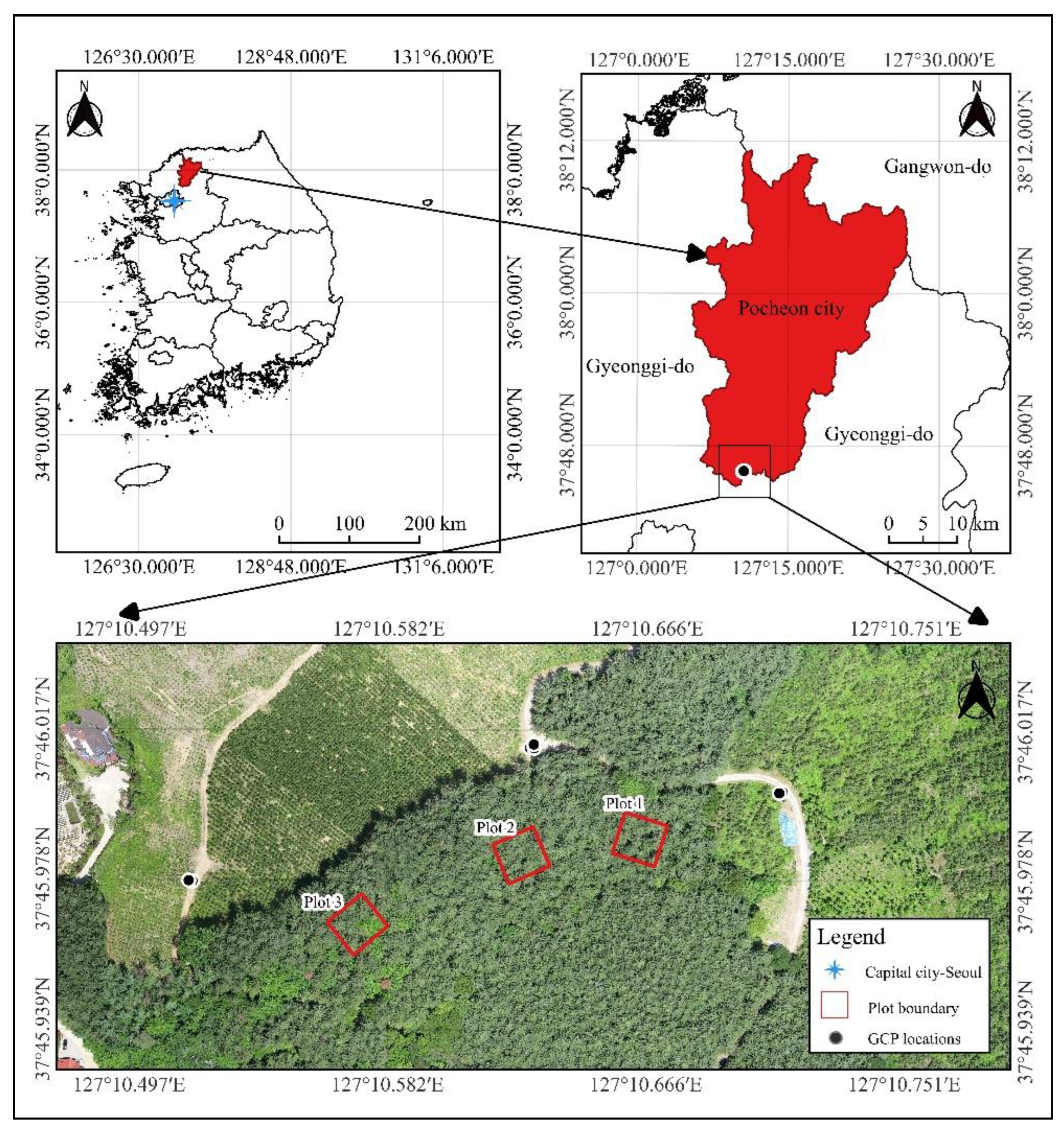
Figure 2.
Flowchart for data processing.
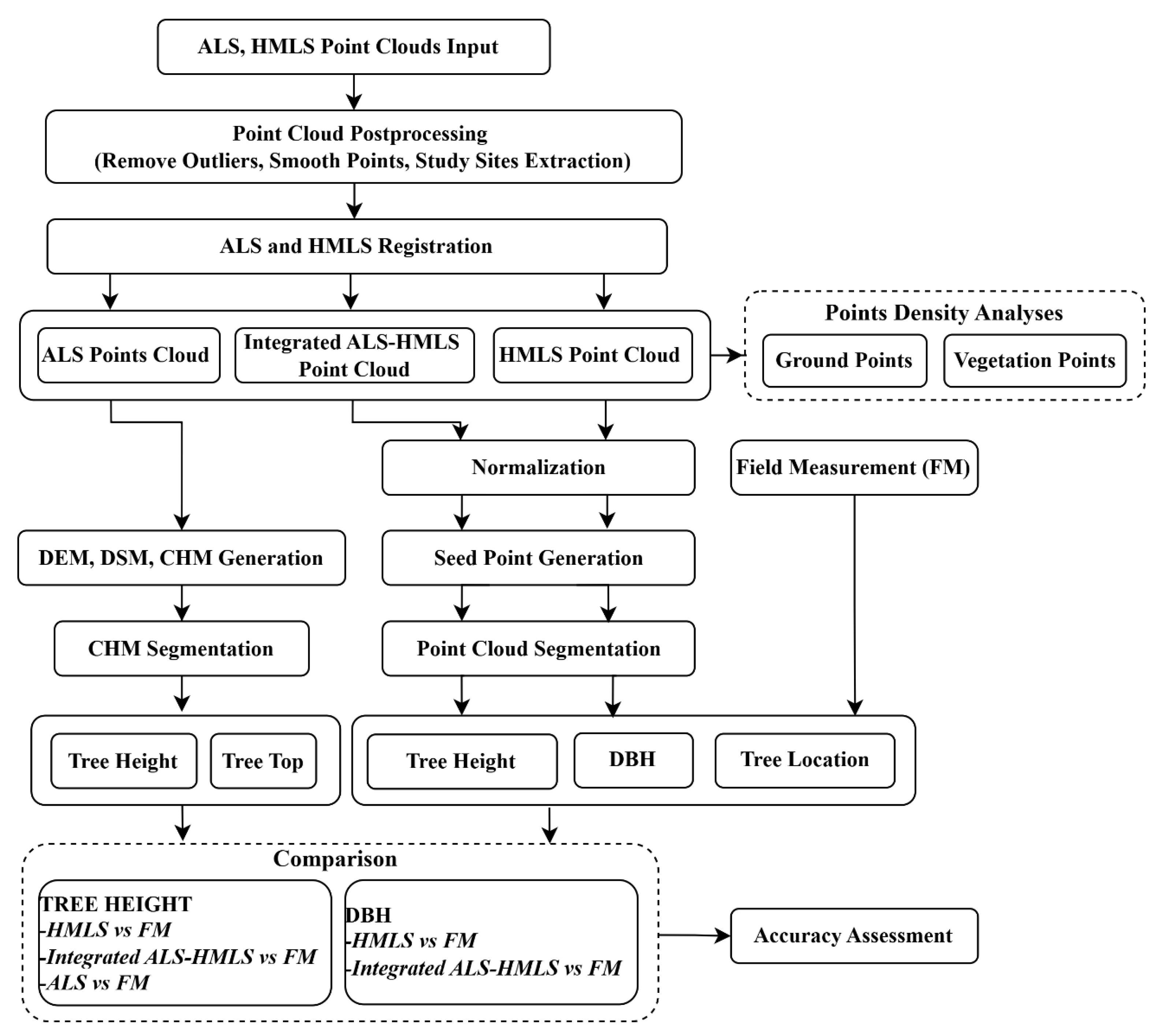
Figure 3.
ALS and HMLS data collection. (A), Pole at 4 corners of plots; (B), Handheld mobile laser scanning; (C), Airborne laser scanner mounted on drone; (D), Static base station on ground.
Figure 3.
ALS and HMLS data collection. (A), Pole at 4 corners of plots; (B), Handheld mobile laser scanning; (C), Airborne laser scanner mounted on drone; (D), Static base station on ground.
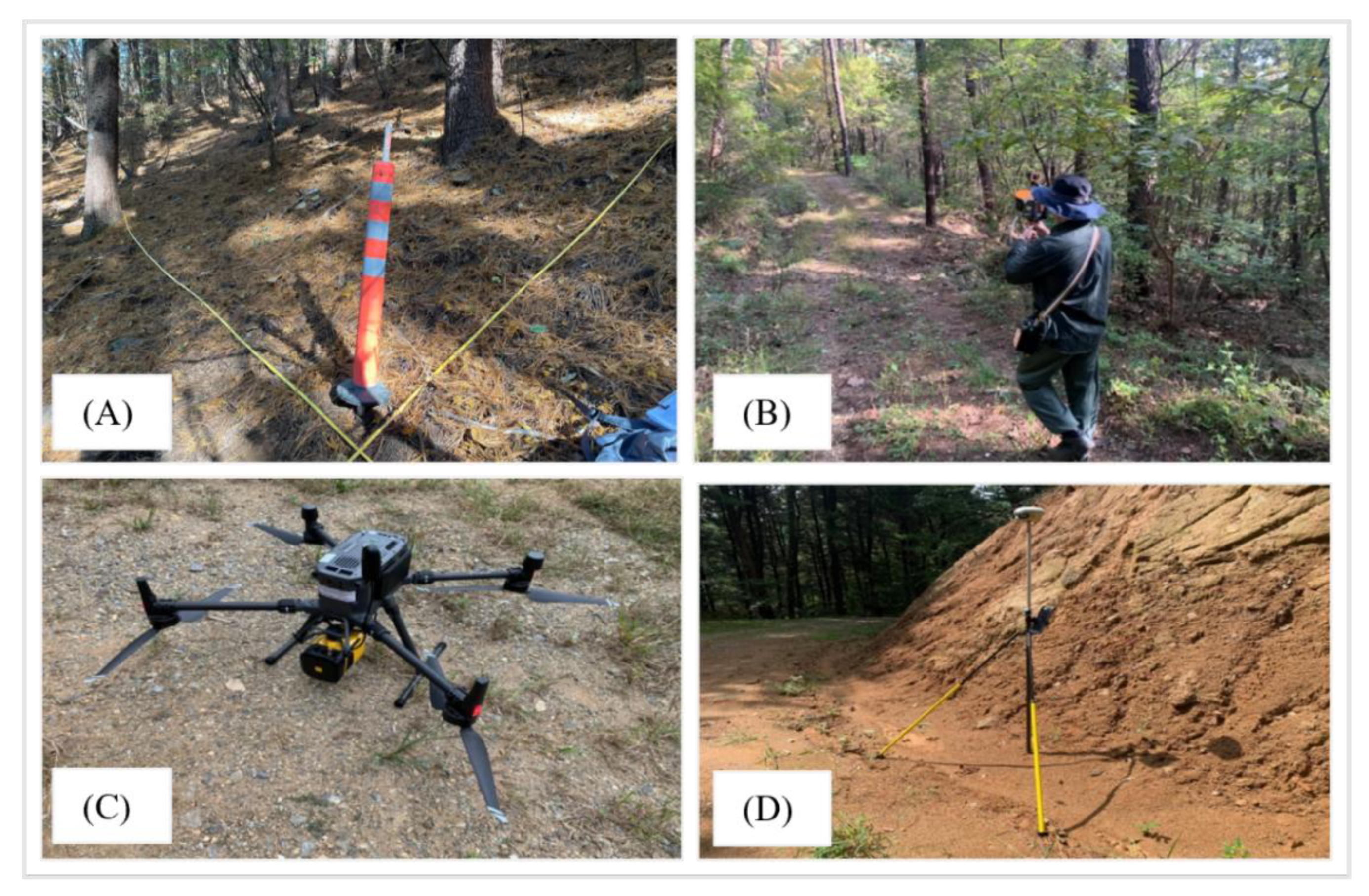
Figure 4.
Tree DBH measurement in 2D (A) and in 3D (B); visual inspection of tree height from HMLS (C).
Figure 4.
Tree DBH measurement in 2D (A) and in 3D (B); visual inspection of tree height from HMLS (C).
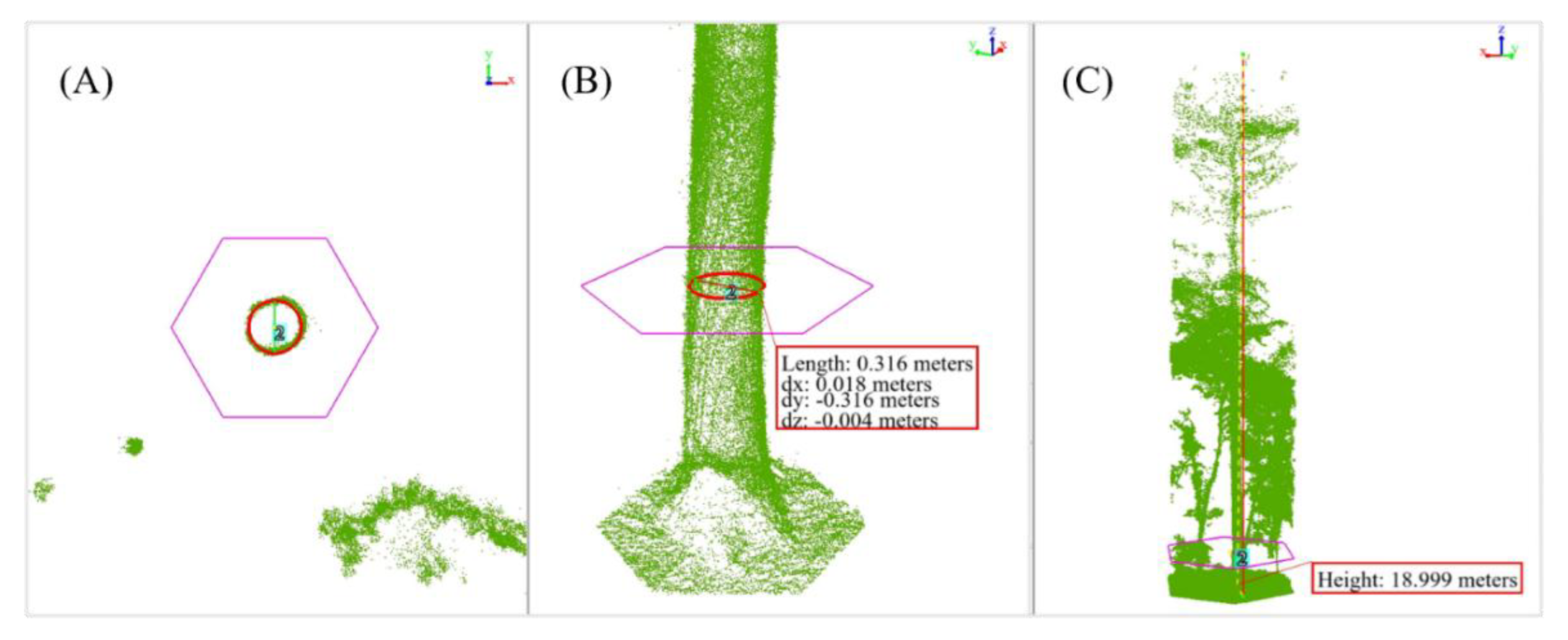
Figure 5.
Example of CHM results including DEM (A), DSM (B), and CHM (C).
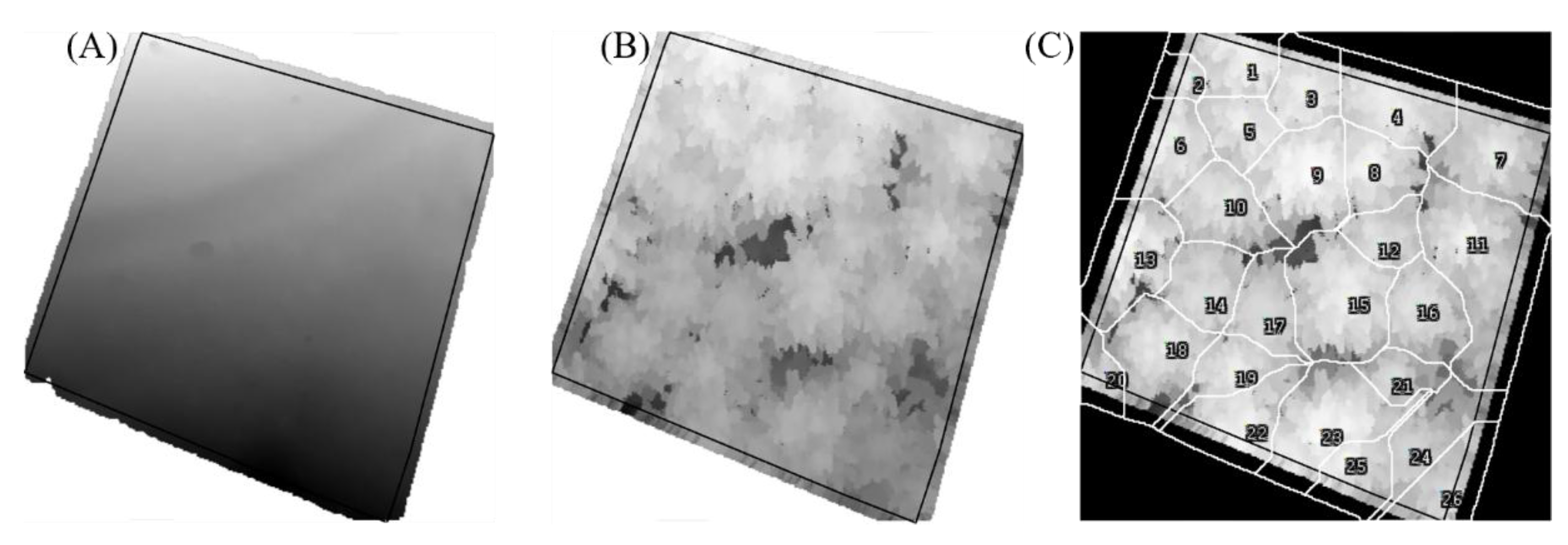
Figure 6.
Result of ALS and HMLS registration (C, F, I, L). Forest point cloud acquired from HMLS (A), ALS (B) and Integrated ALS-HMLS (C); Individual tree in plot 1 acquired from HMLS (D), ALS (E) and Integrated ALS-HMLS (F); Individual tree in plot 2 acquired from HMLS (G), ALS (H) and Integrated ALS-HMLS (I); Individual tree in plot 3 acquired from HMLS (J), ALS (K) and Integrated ALS-HMLS (L). Green color represents HMLS approach, red color represents ALS approach.
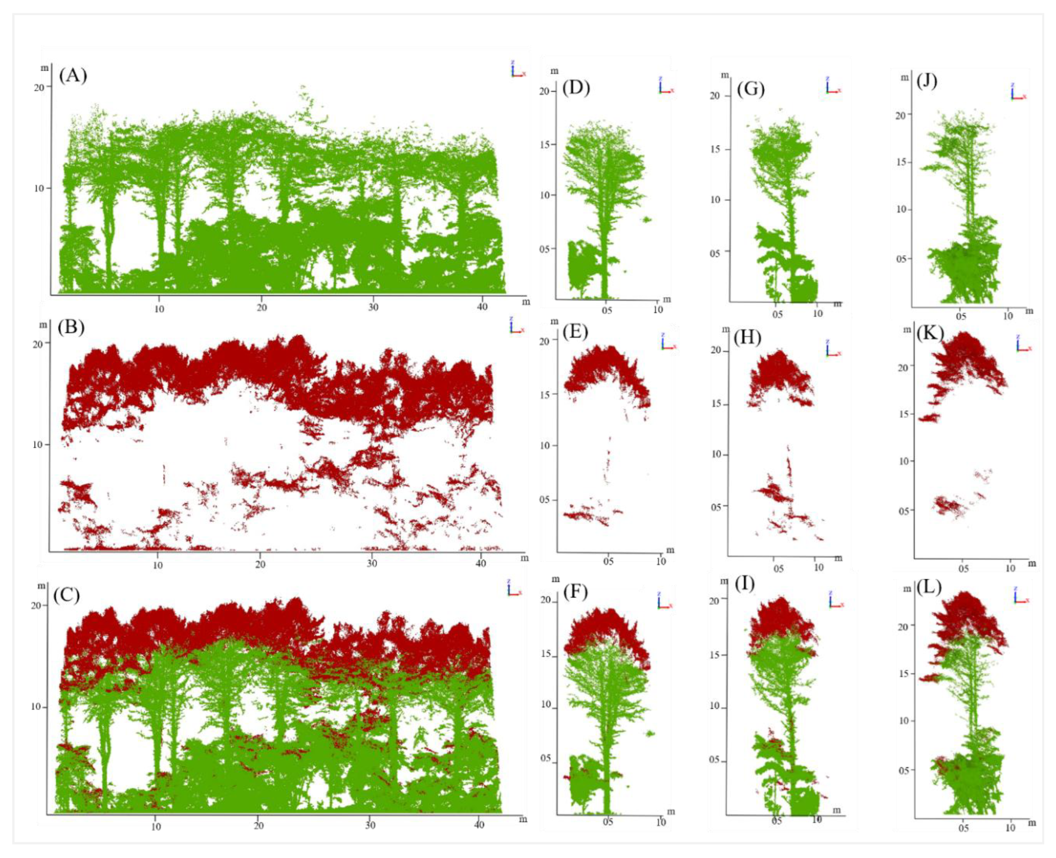
Figure 7.
Comparison of DBH acquired from HMLS and Integrated ALS and HMLS approaches using field measurement (FM) as a benchmark.
Figure 7.
Comparison of DBH acquired from HMLS and Integrated ALS and HMLS approaches using field measurement (FM) as a benchmark.
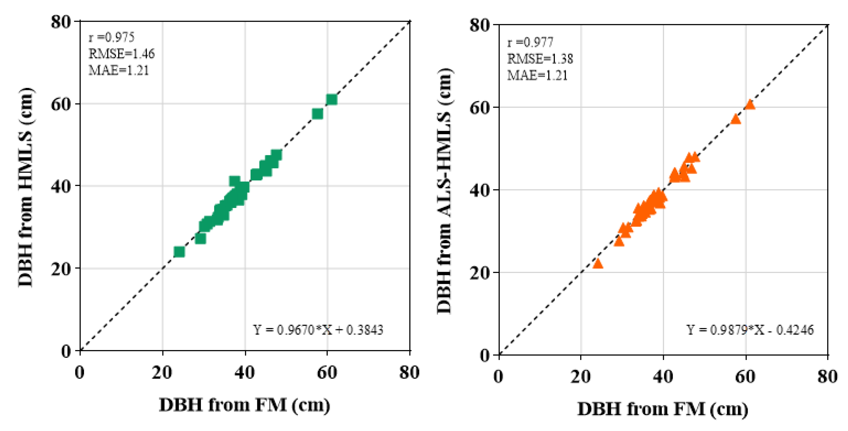
Figure 8.
Comparison of tree height estimations at plot level from Field Measurement against HMLS, ALS, and integrated ALS-HMLS.
Figure 8.
Comparison of tree height estimations at plot level from Field Measurement against HMLS, ALS, and integrated ALS-HMLS.
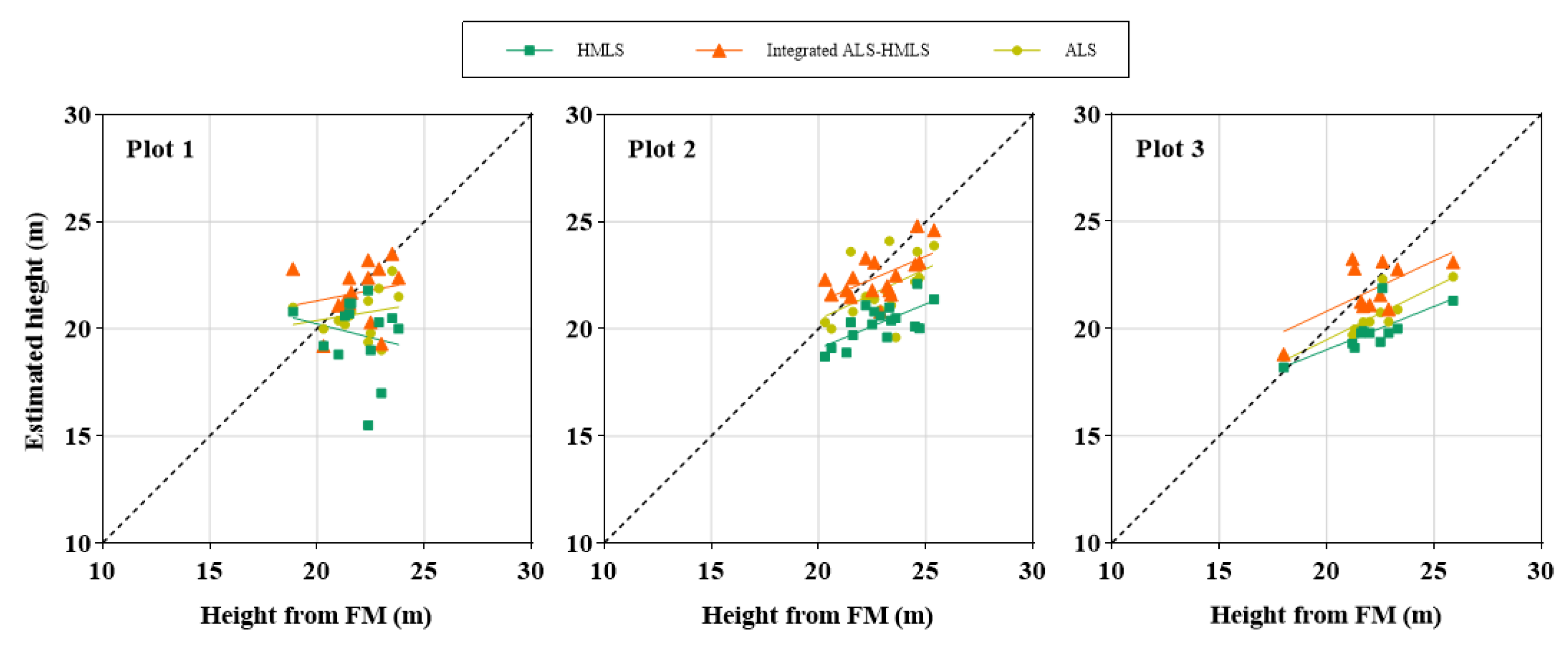
Figure 9.
Residual plots of tree DBHs in each plot. Zero lines are highlighted in red.
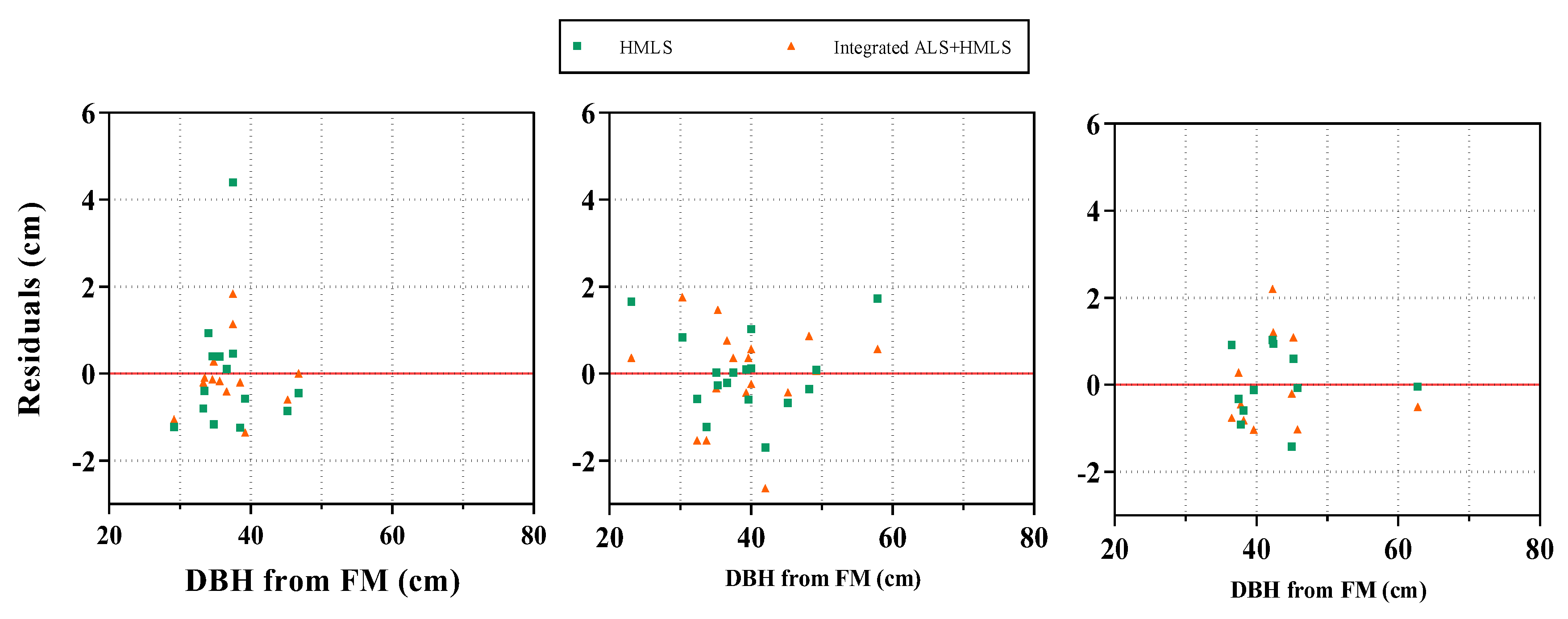
Figure 10.
Residual plots of tree height in each plot. Zero lines are highlighted in red.
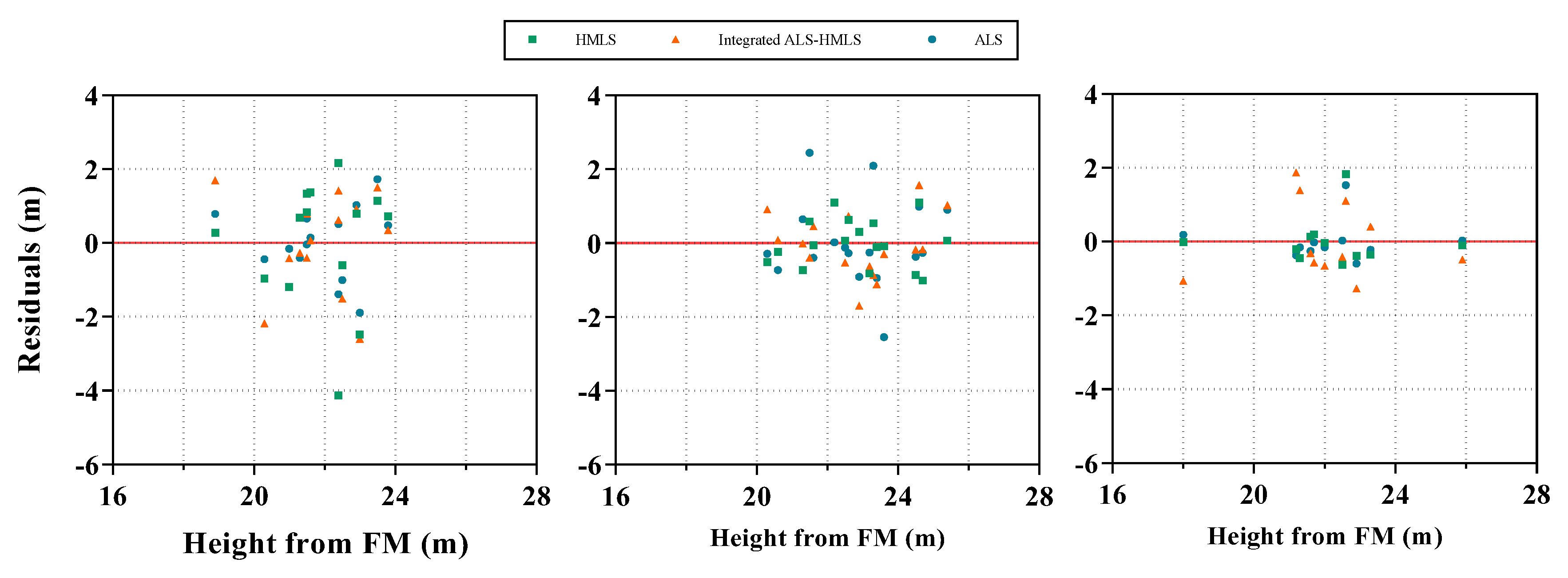
Table 2.
Specification of ZEB Horizon.
| Features | Description |
|---|---|
| Range | 100m |
| Laser | Class 1/ λ 903nm |
| FOV | 360° × 270° |
| Scanner points per second | 300,000 |
| No. of sensors | 16 |
| Vertical angular resolution | 2° |
| Horizontal angular resolution | 0.2° |
| Raw data file size | 25˗50MB/minute |
| Relative accuracy | Up to 6mm |
| Range sensor | Velodyne VLP˗16 |
| Range Rating | Class 1 Eye˗Safe |
| POS system | Integrated SLAM system |
| Operating time | 3hours |
| RGB camera | CAM |
Table 3.
Point cloud density of ground and vegetation point clouds classified from ALS, HMLS and Integrated ALS˗HMLS.
Table 3.
Point cloud density of ground and vegetation point clouds classified from ALS, HMLS and Integrated ALS˗HMLS.
| Point clouds | Plot | ALS | HMLS | Integrated ALS˗HMLS |
|---|---|---|---|---|
| Ground (points/m2) | Plot 1 | 16 | 3,389 | 3,393 |
| Plot 2 | 13 | 2,468 | 2,470 | |
| Plot 3 | 15 | 1,157 | 1,167 | |
| Vegetation (points/m2) | Plot 1 | 2,398 | 21,315 | 23,710 |
| Plot 2 | 2,683 | 26,727 | 29,129 | |
| Plot 3 | 2,793 | 23,594 | 26,356 |
Table 4.
Test results and mean DBH measure by two approaches. Parenthesis represents standard deviation.
Table 4.
Test results and mean DBH measure by two approaches. Parenthesis represents standard deviation.
| Plot | Approaches | Mean DBH |
p˗value (Normality test) |
r coefficient |
p˗value (Correlation) |
|---|---|---|---|---|---|
| 1 | HMLS | 36.22 (4.85) | 0.809 | 0.954 | <0.001 |
| Integrated ALS˗HMLS | 35.97 (4.44) | 0.452 | 0.982 | <0.001 | |
| 2 | HMLS | 37.85 (7.76) | 0.474 | 0.993 | <0.001 |
| Integrated ALS˗HMLS | 37.98 (8.11) | 0.542 | 0.991 | <0.001 | |
| 3 | HMLS | 42.34 (7.02) | 0.002 | 0.952 | <0.001 |
| Integrated ALS˗HMLS | 42.52 (7.1) | 0.007 | 0.936 | <0.001 | |
| All | HMLS | 38.48 (6.99) | 0.013 | 0.975 | <0.001 |
| Integrated ALS˗HMLS | 38.5 (7.13) | 0.015 | 0.977 | <0.001 |
Table 5.
Accuracies of DBH estimation using HMLS.
| Plot | Approaches | RMSE (cm) | rRMSE (%) | Bias (cm) | rBias (%) | MAE (cm) |
|---|---|---|---|---|---|---|
| 1 | HMLS | 1.54 | 4.18 | ˗0.66 | ˗1.79 | 1.23 |
| Integrated ALS˗HMLS | 1.54 | 4.18 | ˗0.66 | ˗1.79 | 1.23 | |
| 2 | HMLS | 1.59 | 4.05 | ˗1.28 | ˗3.28 | 1.40 |
| Integrated ALS˗HMLS | 1.59 | 4.06 | ˗1.16 | ˗2.98 | 1.27 | |
| 3 | HMLS | 1.10 | 2.55 | ˗0.68 | ˗1.58 | 0.91 |
| Integrated ALS˗HMLS | 1.18 | 2.74 | ˗0.48 | ˗1.13 | 1.04 | |
| All | HMLS | 1.46 | 3.70 | ˗0.92 | ˗2.33 | 1.21 |
| Integrated ALS˗HMLS | 1.38 | 3.50 | ˗0.90 | ˗2.29 | 1.21 |
Table 6.
Test results and mean tree height measured by three approaches. Parenthesis represents standard deviation.
Table 6.
Test results and mean tree height measured by three approaches. Parenthesis represents standard deviation.
| Plot | Approaches | Mean Height |
p˗value (Normality test) |
r coefficient |
p˗value (Correlation) |
|---|---|---|---|---|---|
| 1 | HMLS | 19.76 (1.74) | 0.039 | ˗0.191 | 0.514 |
| Integrated ALS˗HMLS | 21.69 (1.36) | 0.245 | 0.186 | 0.524 | |
| ALS | 20.71 (1.01) | 1.000 | 0.217 | 0.456 | |
| 2 | HMLS | 20.27 (0.9) | 0.984 | 0.684 | 0.003 |
| Integrated ALS˗HMLS | 22.47 (1.01) | 0.135 | 0.586 | 0.014 | |
| ALS | 21.78 (1.36) | 0.333 | 0.511 | 0.036 | |
| 3 | HMLS | 19.86 (1.01) | 0.228 | 0.757 | 0.007 |
| Integrated ALS˗HMLS | 21.8 (1.37) | 0.086 | 0.650 | 0.030 | |
| ALS | 20.52 (1.08) | 0.263 | 0.860 | 0.001 | |
| All | HMLS | 19.99 (1.26) | 0.009 | 0.339 | 0.028 |
| Integrated ALS˗HMLS | 22.03 (1.28) | 0.190 | 0.518 | 0.000 | |
| ALS | 21.09 (1.29) | 0.187 | 0.573 | <0.001 |
Table 7.
Accuracy assessment of tree height estimation from HMLS, ALS and Integrated ALS˗HMLS.
| Plot | Approaches | RMSE (cm) | rRMSE (%) | Bias (cm) | rBias (%) | MAE (cm) |
|---|---|---|---|---|---|---|
| 1 | HMLS | 3.13 | 14.31 | ˗2.14 | ˗9.78 | 2.41 |
| Integrated ALS˗HMLS | 1.66 | 7.57 | ˗0.21 | ˗0.98 | 1.04 | |
| ALS | 1.85 | 8.46 | ˗1.18 | ˗5.41 | 1.49 | |
| 2 | HMLS | 2.78 | 12.15 | ˗2.57 | ˗11.25 | 2.57 |
| Integrated ALS˗HMLS | 1.23 | 5.37 | ˗0.36 | ˗1.60 | 1.08 | |
| ALS | 1.73 | 7.57 | ˗1.06 | ˗4.66 | 1.45 | |
| 3 | HMLS | 2.55 | 11.55 | ˗2.23 | ˗10.08 | 2.26 |
| Integrated ALS˗HMLS | 1.40 | 6.36 | ˗0.29 | ˗1.33 | 1.19 | |
| ALS | 1.89 | 8.58 | ˗1.57 | ˗7.12 | 1.70 | |
| All | HMLS | 2.85 | 12.74 | ˗2.34 | ˗10.47 | 2.44 |
| Integrated ALS˗HMLS | 1.43 | 6.41 | ˗0.30 | ˗1.33 | 1.10 | |
| ALS | 1.81 | 8.13 | ˗1.24 | ˗5.54 | 1.53 |
Table 8.
Assessment of ability to produce accurate DBH and tree height from ALS, HMLS and Integrated ALS and HMLS compared to Field Measurement.
Table 8.
Assessment of ability to produce accurate DBH and tree height from ALS, HMLS and Integrated ALS and HMLS compared to Field Measurement.
| LiDAR approach | Field Measurement | |
|---|---|---|
| DBH | Height | |
| ALS | NA | High |
| HMLS | High | Medium |
| Integrated ALS and HMLS | High | High |
NA, Not Available.
Disclaimer/Publisher’s Note: The statements, opinions and data contained in all publications are solely those of the individual author(s) and contributor(s) and not of MDPI and/or the editor(s). MDPI and/or the editor(s) disclaim responsibility for any injury to people or property resulting from any ideas, methods, instructions or products referred to in the content. |
© 2025 by the authors. Licensee MDPI, Basel, Switzerland. This article is an open access article distributed under the terms and conditions of the Creative Commons Attribution (CC BY) license (http://creativecommons.org/licenses/by/4.0/).
Copyright: This open access article is published under a Creative Commons CC BY 4.0 license, which permit the free download, distribution, and reuse, provided that the author and preprint are cited in any reuse.


