Quantitative and Spatially Explicit Clustering of Urban Grocery Shoppers in Montreal: Integrating Loyalty Data with a Synthetic Population

1. Introduction

Geographically explicit models have played an instrumental role in advancing our understanding of spatially explicit, dynamic socio-economic systems. By incorporating spatial data and human decision-making processes, these models allow researchers to capture the nuanced ways in which individuals, communities, and larger populations interact within defined geographic contexts [27]. The selection of a grocery retail store by customers living in an urban environment is one such complex socio-economic problem that has a significant spatial aspect, and one in which customers and retailers interact dynamically. While spatial elements such as proximity to stores can directly influence a customer’s behaviour, it is also driven by marketing strategies, which are themselves informed by knowledge of their customer base, their profiles, needs, and habits [34]. Because of the complexities involved, only geographically explicit modelling enables a proper assessment of the diverse factors that drive consumer decisions, while also providing a platform for simulating potential policy interventions or market changes [6].

Amongst geographically explicit modelling strategies, Agent-Based Models (ABM) have emerged as a widely adopted approach due to its capacity to simulate complex systems by capturing the behaviours and interactions of autonomous decision-making agents within a spatial context [27,29]. Within an ABM, each agent operates according to a set of predefined rules, yet the collective behaviours of these agents can give rise to emergent patterns that may be difficult to predict using traditional modelling approaches [17]. When combined with Geographical Information Systems (GIS), ABM becomes particularly powerful [9]. GIS data supplies the spatial and environmental context, while ABM manages the cognitive and behavioural rules of agents, creating simulations that more closely represent the real-world processes.

However, a key requirement for accurate and reliable ABM simulations lies in constructing heterogeneous agent profiles [28]. Heterogeneity reflects the diversity among individuals in terms of demographic attributes, socioeconomic status, behavioural tendencies, and preferences [33]. In the context of food retail choice, for instance, individuals may differ in their household size, income, dietary preferences, vehicle ownership, and daily commuting patterns—all of which can greatly influence where and when they choose to shop for groceries. By incorporating such variation, model builders can produce simulations that better approximate real-world decision-making processes.

Despite the clear importance of agent heterogeneity, acquiring detailed, individual-level data to build such profiles can be challenging. Privacy regulations, for example, often limit the extent to which personally identifiable information can be shared or used for research purposes [12]. In addition, the cost and logistics of large-scale surveys may be prohibitive, and secondary data sources may not always offer the level of granular details required to construct agent profiles. These obstacles have led researchers to seek creative solutions for data gathering and synthesis. When real-world data is sparse or incomplete, synthetic approaches—where populations are generated or augmented based on statistical methods—can fill some of the gaps [1,18,35].

Synthetic population data is generated through techniques that approximate the demographic composition of actual populations. By relying on census information or large-scale surveys, synthetic populations are constructed to have the same statistical characteristics as real-world groups, including household size, age distribution, and income brackets [1]. These methods have been widely applied in ABM research to represent agent diversity without obtaining personally identifiable information [7]. Consequently, synthetic population datasets serve as an invaluable resource for modellers who wish to represent a range of demographic attributes while respecting data privacy constraints.

Secondary data sources, such as loyalty membership program data, can be combined with synthetic population data to help augment information about customer choice. Since the 1990s, such loyalty programs have become popular in the retail sector. These programs allow retailers to track an individual’s interaction with their stores, and often capture valuable information about consumer behaviours, such as the residential addresses of customers, types of products purchased, the frequency of store visits, and the total amount spent per visit [4]. While these data are typically anonymized and only provide limited information on the social-demographics to protect individual identities, they can still offer robust insights into the purchasing patterns of diverse customer segments.

Therefore, there is strong potential for integration of these two types of data, loyalty program and synthetic population, to develop richly detailed and heterogeneous agent profiles. Loyalty program data provide anonymized information about consumers’ behaviour, revealing purchasing habits and frequency, while synthetic population data addresses the need for demographic and socioeconomic attributes for constructing a broader customer landscape. By bringing these complementary datasets together based on residential postal codes, researchers can overcome many of the limitations posed by each individual data source. Rather than relying solely on synthetic demographic profiles that may or may not accurately reflect actual consumer behaviour, or exclusively on loyalty program data that may lack detailed demographic attributes, a combined dataset helps produce a holistic representation of consumers in a specific urban environment.

However, raw data integration alone may not be sufficient to understand and exploit the underlying heterogeneity within a consumer base, which can yield a large database without identifying any patterns. Clustering methods come into play as a powerful analytical tool for grouping individuals who share similar demographic, socioeconomic, and behavioural attributes [21], and further help build the computational representation of this typology as specific “agent types” in an ABM [30]. This clustering process not only assists modellers in identifying meaningful segments within large, complex datasets, but also aids stakeholders, such as retailers, urban planners, and policymakers, in grasping the diversity of consumer types across a geographic areas. Through the segmentation, decision-makers can develop tailored strategies by informing marketing strategies, store location planning, or targeted policy interventions.

The combined approach outlined above overcomes two principal limitations of most existing approaches to grocery customer clustering. First, they frequently rely on a single data source—either behavioural data (e.g., loyalty card data) or socioeconomic data [11]. In studies that emphasize socioeconomic data, census information is commonly employed rather than a synthetic population, thereby restricting customer variability and reducing agent heterogeneity in agent-based models. Consequently, it becomes difficult to capture a comprehensive understanding of customer behaviour. The second limitation is the lack of quantitative and geographical perspectives of customer clusters. For instance, although Sturley et al. [32] created customer segmentation for grocery purchases that incorporates clear geographical insights, the primary focus on model building precluded the inclusion of quantitative representations of clusters and socioeconomic variables. This can limit the utility and interpretability of segmentation for broader analytical or practical applications.

Building on these observations, this paper integrates loyalty program data with synthetic population data and applies clustering methods to enhance our understanding of grocery customers. By bridging the gap between single-source studies and those lacking quantitative geographic insights, this work seeks to capture both behavioural and socioeconomic dimensions of customer segments within a spatially explicit context. We argue that such an integrated approach not only enriches ABM simulations by representing heterogeneous consumer profiles more accurately, but also provides guidance for retailers, urban planners, and policymakers aiming to make data-driven decisions. In the remainder of this paper, we outline our methodology and present a quantitative view of customer segments.

2. Methods

2.1. Study Area

Our study area is the island that makes up the city of Montreal. Encompassing approximately 500.6 km², Montreal is the largest city in Quebec and the second largest in Canada. According to Statistics Canada [31], the city is home to over 1.7 million residents across 816,340 occupied private dwellings. Montreal’s diverse demographic landscape offers a unique opportunity to investigate population heterogeneity, thereby facilitating the derivation of distinct customer clusters. Figure 1 illustrates the location of our study area, the city of Montreal, and the spatial distribution of loyalty program members as their total count in each Dissemination Area (DA), the smallest standard geographical unit of the Canadian census.

2.2. Data Sources

This study utilizes two datasets: a synthetic population and customer loyalty program data, the latter obtained from a prominent local retail chain operating grocery stores on the island of Montreal, to construct a typology of customers. The synthetic population data are derived from the Syntheco project at the McGill Centre for the Convergence of Health and Economics (MCCHE) [13]. The Syntheco project aims to establish a synthetic ecosystem for the analysis of complex human individual behaviours, with the creation of synthetic populations for Canadian and US contexts from Census data as a key milestone. For this paper, we specifically utilize the Canadian synthetic population to ascertain the demographic profiles of customers from the loyalty dataset. This synthetic population is crafted using geographical boundary structures, data from the 2016 Canadian Census, and household data from the Public Use Microdata Files (PUMF) employing the Iterative Proportional Fitting (IPF) algorithm. Consequently, all attributes from the PUMF data are replicated in the synthetic population. In this synthetic population, individuals are linked with their corresponding households and each household has the coordinates to illustrate their geolocation [13].

The loyalty program dataset is sourced from a chain that operates retail stores with a focus on selling food items across Montreal and the province of Quebec, and covers 32 months from February 2015 to September 2017. It encompasses various types of data, including each transaction made by members, store details, and member information pertaining to their declared residential postal code. The transactional data contains detailed entries typically found on a receipt, such as timestamps, transaction IDs, total spending amounts, store IDs, and loyalty card IDs. These elements enable us to analyze customer behaviour by joining the datasets. However, the loyalty program data lacks personal information, with only a postal code available. This postal code presumably identifies the residential postal code of the member.

2.3. Connecting the Loyalty Data with the Synthetic Population

In order to conduct an analysis of consumer behaviours, our study focuses on transactional data for each member available in the loyalty program dataset. This data is foundational, as it is explicitly tied to individual loyalty IDs, providing a granular view of purchasing patterns by each member enrolled in the program. Based on Sturley et al. [32], we identify several critical behavioural metrics: frequency of store visits, distance to the most frequently visited store, distance to the nearest store, and timing of visits (differentiated by weekday/weekend and daytime/evening). These indicators are selected due to their proven relevance in understanding the landscape of consumer shopping preferences and patterns.

However, the mere analysis of transactional data can be limiting, as Carpenter & Moore [5] suggest that demographics are a significant determinant of consumer shopping behaviour. Unfortunately, our primary dataset—the loyalty program data—does not include comprehensive demographic details, with the exception of postal codes associated with each member. This limitation necessitates an alternate approach to deduce a more complete profile of our consumers. To address this gap, we leverage synthetic population data, which provides detailed demographic insights absent in our primary dataset.

Given the scale of our study, involving 295,632 loyalty cardholders, we employ a average nearest neighbour approach to attach demographic data to each loyalty program member. Specifically, we use the geographic boundary file of postal codes to find the five closest households within the synthetic population database for each loyalty member. This proximity-based matching is predicated on the assumption that individuals in close geographical proximity share similar demographic characteristics.

To facilitate a manageable and effective analysis, we sub-select a set of demographic attributes from the synthetic population. The original PUMF dataset includes 99 variables, which is unwieldy for direct analysis. Therefore, selecting variables that are most pertinent to retail consumer behaviour carefully is significant in this approach. Demographic attributes to be used for clustering purposes were selected from the PUMF dataset based on these criteria: (1) direct relevance to retail consumer behaviour and (2) spatially distributed. Considering the uncertainties introduced by proximity-based matching, we seek an attribute that is both spatially distributed and influential in purchase decisions. Consequently, we select individual gross income as this attribute, given its documented geographical variation in Montreal [22] and its established influence on grocery shopping behaviour [2,15,20]. Other variables either do not meet these requirements or are not explicitly specified in the PUMF. This integrated dataset thus serves as a foundation for subsequent analytical phases, where we delineate distinct customer segments based on this combined dataset.

Within the combined dataset, the following eight variables are considered: individual gross income, average spending per transaction, frequency of store visits, distance to the store they visit most frequently, distance to their nearest store, the total number of stores they visited, the percentage of their shopping done on weekend and in the evening. These variables were deemed suitable to demonstrate demographic and behavioural information about each customer with available transaction records in the database.

2.4. Typology Generation

For the purpose of generating a customer typology, we employ the K-means clustering algorithm to organize the integrated loyalty program data into distinct groups. The decision to use K-means over alternative clustering methods such as K-medoids or DBSCAN is informed by its demonstrated efficacy in customer segmentation tasks. According to Brahmana et al. [3], K-means provides a superior level of validity in defining customer segments compared with other approaches. In addition, because all our attributes are continuous or converted to continuous (e.g. from the time segments of shopping to the percentage of shopping time), K-means is well suited to clustering the integrated dataset [16]. Further, since our attributes are all numerical , we introduce a log transformation to those with pronounced skew (skewness > 0.75), a strategy used to enhance the performance of clustering algorithms, such as the K-means used in this study [26].

To ascertain the optimal number of clusters, we apply the elbow method. This technique involves plotting the explained variance as a function of the number of clusters and selecting the point where the increase in variance explained becomes less pronounced, resembling an "elbow" [10]. The results of this analysis are depicted in Figure 2. To assess the quality of our clustering, we utilize the sum of squares error (SSE). Notably, a distinct elbow is observed at the seven-cluster mark, suggesting that segmenting the data into seven categories will yield the most meaningful and actionable insights.

3. Results

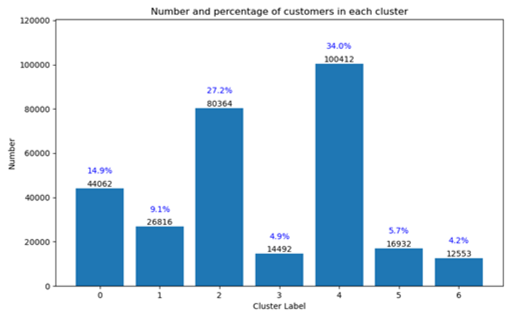
Following segmentation using the k-means algorithm, the 295,631 customers in the loyalty dataset are clustered into seven groups. As shown in Figure 3, cluster 2 and 4 have the largest number of total individuals among all the groups, and they together contribute more than half of the total customers recorded in the loyalty dataset. On the contrary, cluster 3, 5 and 6 have the lowest numbers at 10,000 individuals, and clusters 0 and 1 range between 20,000 to 40,000 individuals. Table 1 illustrates the descriptive statistics of all numerical variables for generating the typology. In the following part, we will describe these clusters from the perspectives of each attribute.

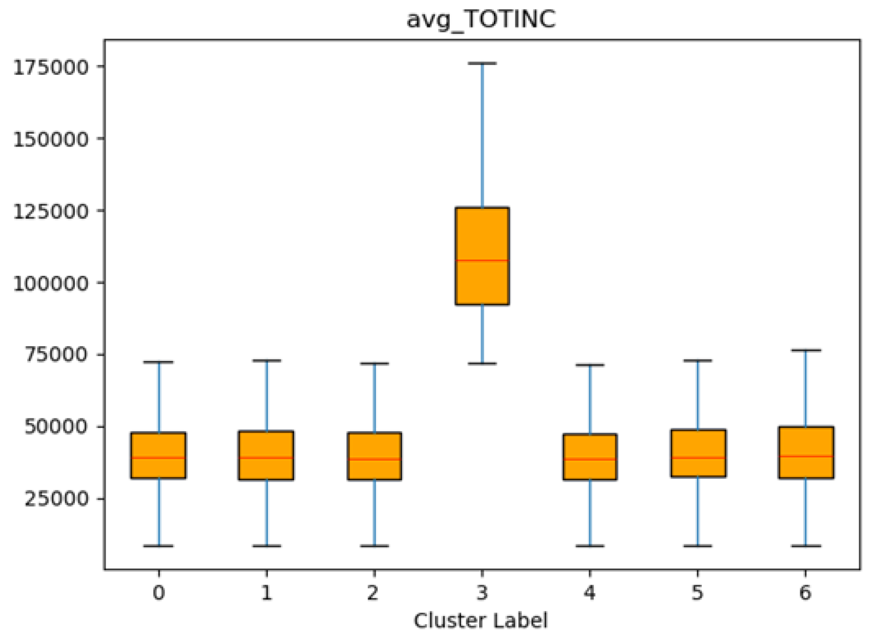
3.1. Total Income

Total individual gross income is a variable obtained from the synthetic population, and according to Prased [25], income is the most frequently mentioned variable influencing customer choice in markedly literature. Therefore, we believe including this attribute is imperative to carrying out proper customer segmentation in terms of shopping choices.

Table 1 and Figure 4 illustrates the total income of each segment of customers. The average income value of most clusters is approximately $40,000 to $50,000, except for cluster 3. The mean value of cluster 3 is the highest at $110,898.73, while also having significant variability, which is around 2 times that of other clusters.

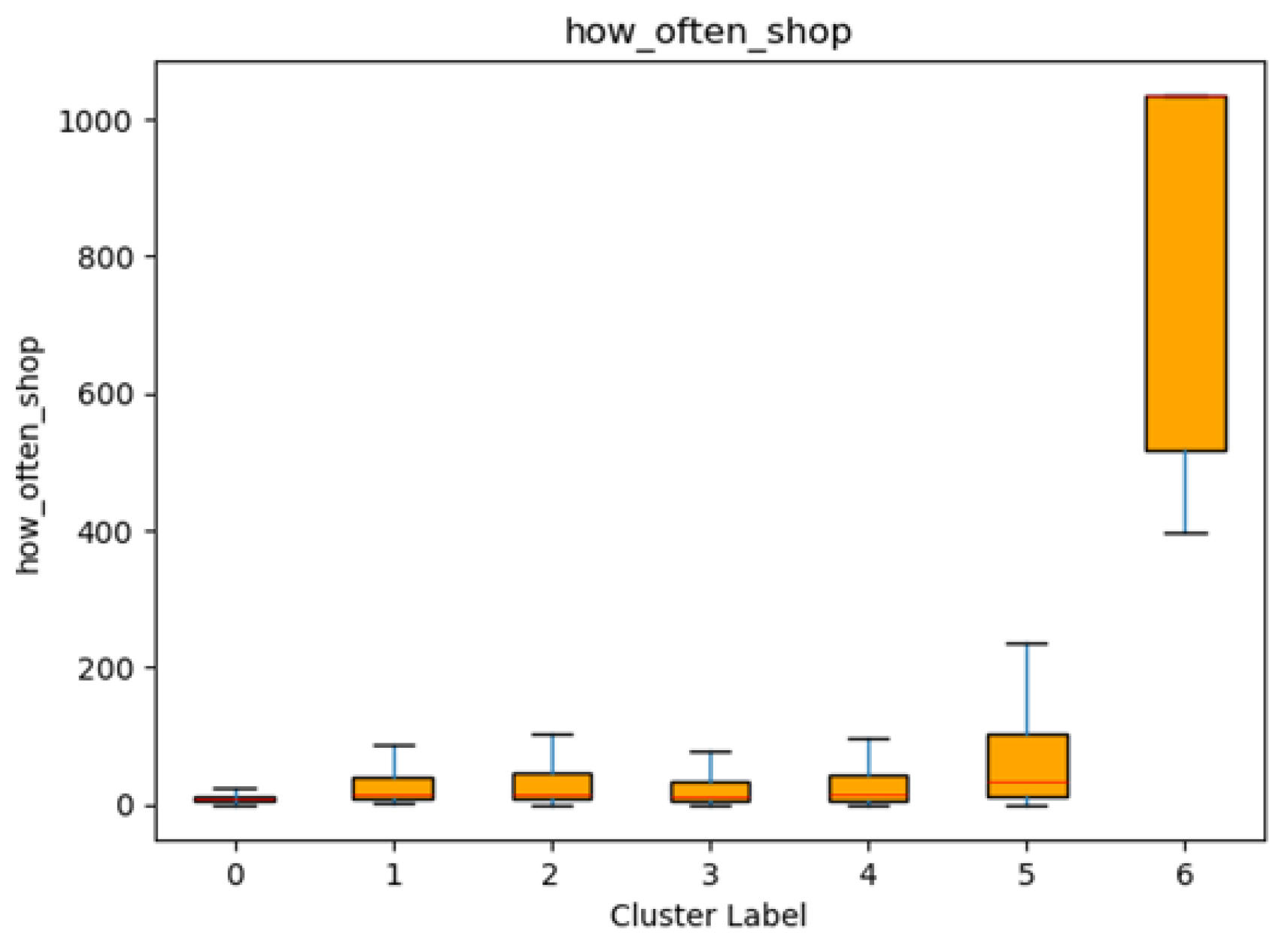
3.2. Frequency of Store Visits

Based on the transaction records in the loyalty dataset, the frequency of customer shopping in a total period “F” can be calculated as the number of times a customer visits any store of the chain during the total activation period of loyalty cards, which is calculated through the following equation:

$$F={\displaystyle \frac{Totalactivationperiodindays}{Thenumberoftotalvisits}},$$

(1)

The variable “F” thus captures the frequency of visits, e.g., an F value of “7” indicating one visit weekly. In the clustering process, this behavioural attribute is also included in the K-means method, and we can examine this variable by clusters.

Table 1 and Figure 5 provide a detailed comparison of median “days per store visit” across the seven identified customer segments, revealing notable differences in shopping frequency. Cluster 0 stands out as the most frequent shopper segment, with a median interval of only 7.39 days between visits, which means they visit stores every week. By contrast, Cluster 6 has a markedly higher median interval of 1034 days, making its members the least frequent group in the analysis, and it also has the fewest number of customers. This thus identifies this cluster as infrequent visitors who shopped less than 5 times over their entire activation period. Positioned between these two extremes, Clusters 1, 2, 3, and 4 exhibit moderate intervals (ranging from 12.77 to 16.00 days), indicating middle ground in terms of shopping frequency (i.e., approximately once every 2 weeks on average). They also make up the largest group of individuals. Cluster 5, at 34.47 days per visit (i.e., approximately once per month), is substantially less frequent than Clusters 0 through 4, but still far below the considerable gap shown by Cluster 6.

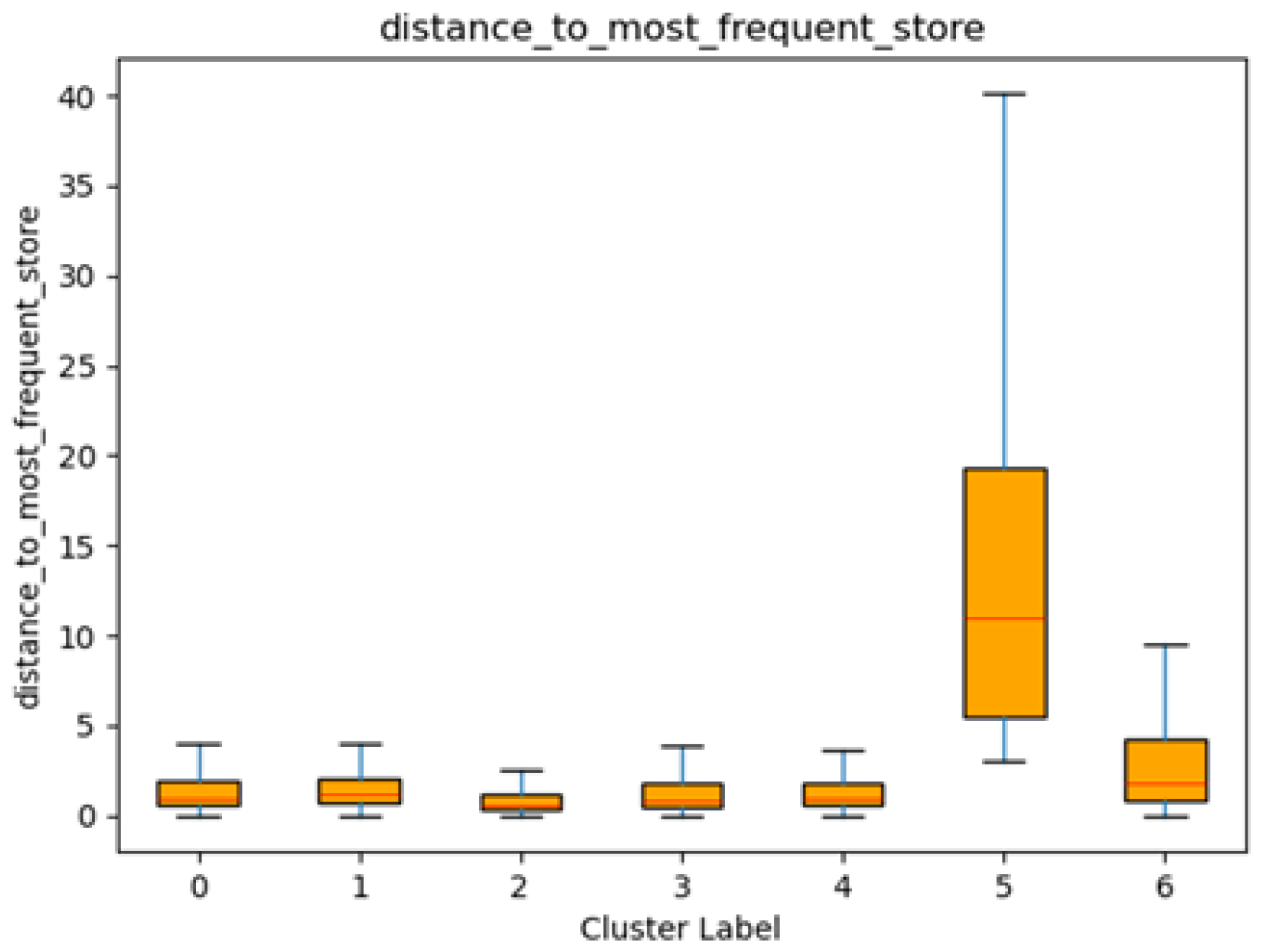
3.3. Distance to Their Most Frequently Visited, as Well as Nearest Store

To examine whether distance influences customers’ store choices, we analyzed the distances to both the most frequently visited store and the nearest store within each customer segment. Distances were obtained from the loyalty dataset, given the well-established impact of geographical proximity on consumer decision-making. Table 1 provides the statistics of the distances between customers and their most frequently visited store. Overall, Clusters 0–4 exhibit relatively small mean distances, ranging from approximately 1.20 to 1.74 km, suggesting that customers in these segments tend to frequent a store that is geographically close to them. Cluster 2 has the smallest mean distance (1.20 km), indicating that these customers strongly prefer nearby stores.

By contrast, Cluster 5 stands out with a much larger mean distance (14.27 km) and the highest standard deviation (11.09), implying that some customers within this segment routinely travel farther to shop. Cluster 6 has a moderately larger mean distance than Clusters 0–4 (3.62 km), and its higher standard deviation (4.88) also suggests more variation in store choice based on location. Figure 6 depicts the box plots for these distances by cluster, highlighting the pronounced difference in distance for Cluster 5 in comparison to the other segments.

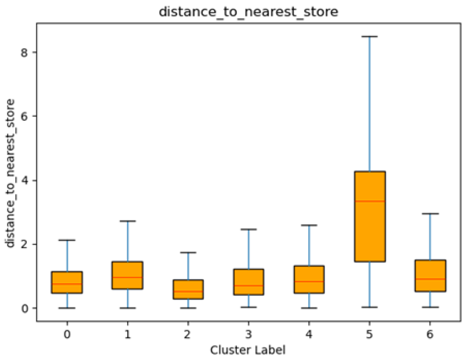
Based on the customer and store location, the average distance to the nearest store that each cluster’s members have visited can also be summarized and compared with the most frequently visited store. In general, Clusters 0–4 again show smaller mean distances, all below or around 1 km. Notably, Cluster 2 has the smallest mean distance (0.66 km), suggesting that these customers tend to have at least one store located very close to their residential postal codes.

Cluster 5 still registers the greatest distance (3.18 km) to the nearest store, though notably smaller than its distance to its most frequently visited store. Cluster 6 also has a higher mean distance compared to most other clusters (1.20 km), with a relatively large standard deviation of 1.02. These patterns suggest a greater willingness amongst individuals in Clusters 5 and 6 to travel farther—even for the nearest store—compared to the other segments. Figure 7 illustrates these distances via box plots, reflecting the comparatively wide distribution of distances for Cluster 5 and the moderate distances for Cluster 6.

Overall, these findings suggest that while most customer segments prefer stores located close to their primary residence or routine travel paths, certain segments (notably Clusters 5 and 6) are more likely to travel longer distances—whether to their most frequently visited store, or to other stores in the chain nearest to them—indicating distinct shopping preferences and behaviours within these groups.

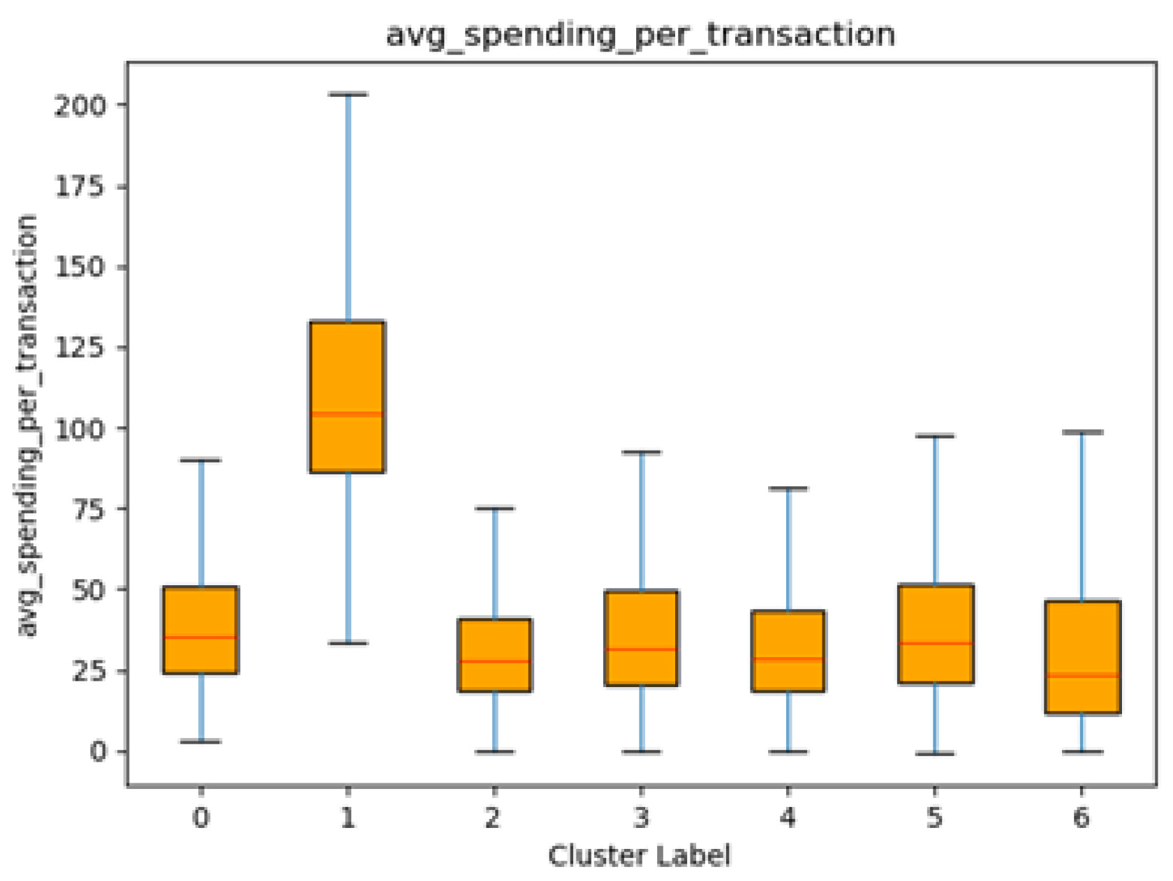
3.4. Average Spending per Transaction

By examining the average spending per transaction, we can identify key differences in how much customers typically spend during each visit, revealing the sales value of each cluster to the retailer. This analysis helps determine which groups are more inclined to spend more, and those that exhibit more conservative purchasing habits, allowing for targeted strategies and individual simulation that align with each segment’s distinct financial behaviours.

The spending patterns vary notably across the clusters, with Cluster 1 standing out due to its significantly higher mean spending ($115.71) compared to other clusters, whose average spending ranges between $31.72 and $39.75. Cluster 1 also shows a relatively high standard deviation ($47.83), indicating greater variability in spending compared to other segments.

Figure 8 displays box plots of the average spending per transaction by cluster, further highlighting the disparities among the clusters. Most clusters exhibit compact distributions with lower median spending values and moderate variability, suggesting consistent spending behaviours within these segments. In contrast, Cluster 1 shows a higher median and broader spread, reinforcing the data that this segment spends considerably more per transaction than others. The spread observed in Cluster 1 suggests that customers in this segment are more likely to engage in higher spending transactions.

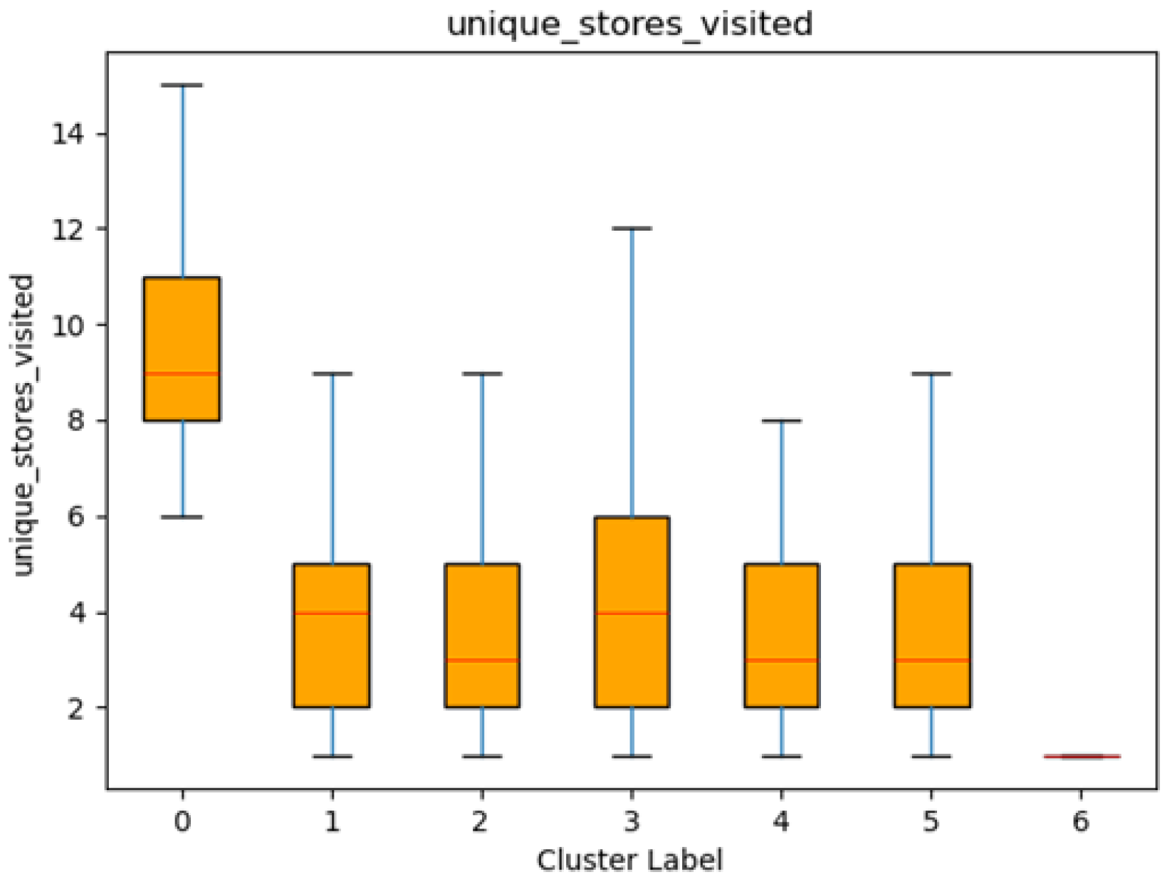
3.5. The Number of Unique Stores Visited

Examining the number of unique stores each customer visits provides additional valuable insights into their shopping preferences. A higher count may indicate more exploratory or variety-seeking tendencies, whereas a lower count suggests a narrower focus on specific stores, or very low frequency of shopping. In this section, compare the number of unique stores visited using descriptive statistics and a box plot visualization.

As shown in Table 1 and Figure 9, Cluster 0 stands out with the highest mean number of unique stores visited (9.93) and a relatively wide range (std = 3.09). By contrast, Cluster 6 exhibits the lowest mean (1.11) and the narrowest spread (std = 0.31), suggesting that members of this segment tend to visit very few, if any, additional stores apart from their “usual” store. Based on the results of shopping frequency mentioned earlier, we also know that Cluster 6 consists of extremely low-frequency shoppers. This helps explains the narrow choices of store visits, as this cluster is made up of very infrequent shoppers

In between these extremes, Clusters 1, 2, 3, 4, and 5 have average values ranging from 3.40 to 4.50, indicating moderate number of different stores visited. These patterns are also evident in the box plots, where each cluster’s median, quartiles, and any outliers visually reflect the variability observed in the table. Overall, the data suggest that Cluster 0 customers explore visiting many different stores, whereas Cluster 6 shoppers appear the most limited in their store visits.

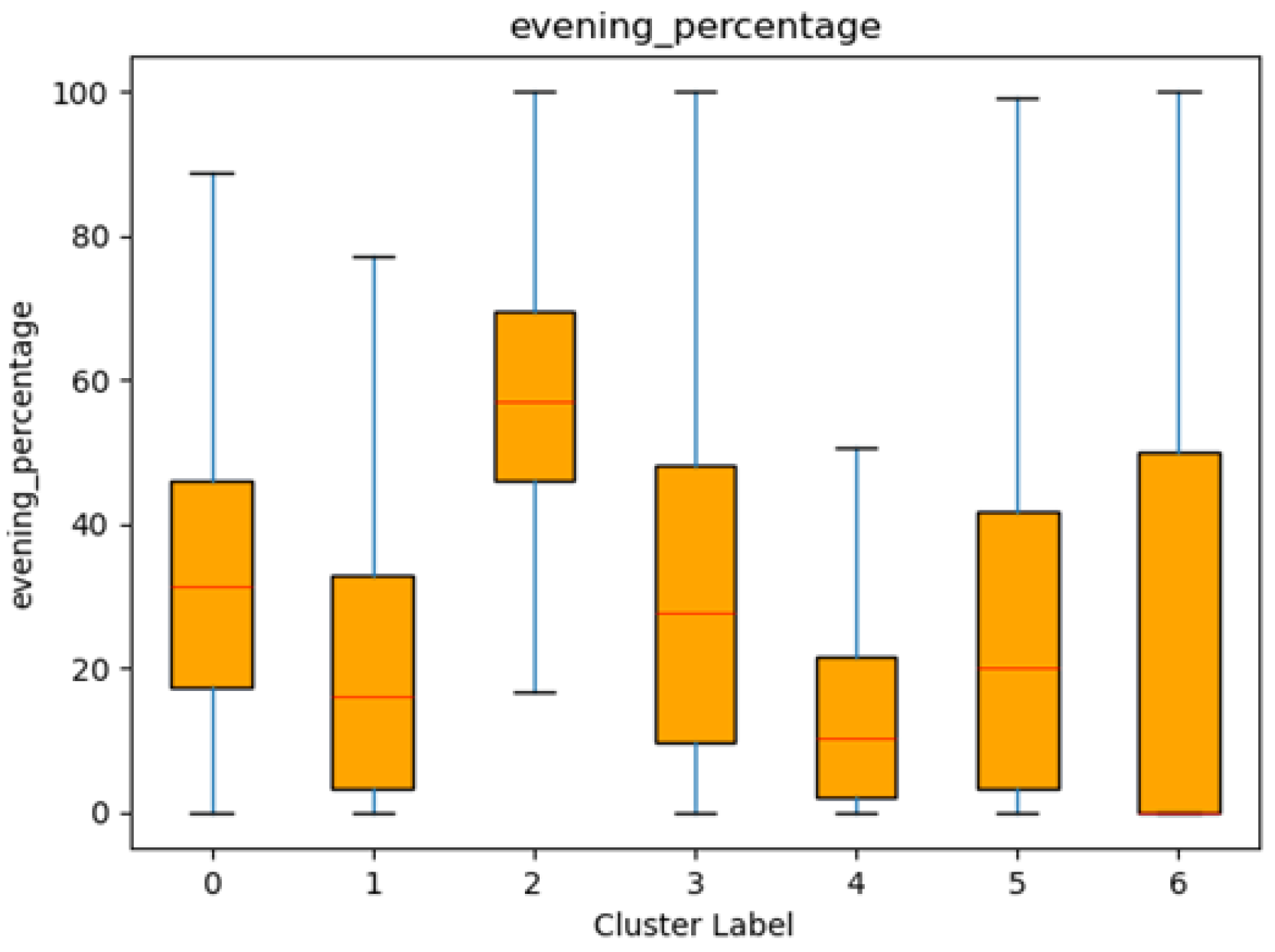
3.6. The Percentage of Shopping Done in the Evening

To further examine customer behaviours, we analyzed the proportion of shopping that occurs during the evening. Cluster 2 demonstrates the highest mean percentage of evening shopping at 58.77%, with a relatively low standard deviation (16.66) indicating that most customers in this segment consistently prefer to shop in the evening. Cluster 0 follows with a mean of 32.39%, and Cluster 3 has a comparable mean of 30.76%, though both clusters display wider variability in their distributions, as reflected by their higher standard deviations.

In contrast, Cluster 4 exhibits the lowest mean percentage of evening shopping at 12.64%, suggesting that these customers are least likely to shop in the evening. Cluster 1 also shows a relatively low mean (20.49%) but is more spread out, as indicated by a standard deviation of 19.67. Clusters 5 and 6 occupy the mid-range, with mean values of 25.67% and 27.76%, respectively. The particularly high standard deviation (41.94) for Cluster 6 suggests that while some customers do a considerable portion of their shopping in the evening, others in this cluster are not so consistent.

The box plots in Figure 10 illustrate these differences clearly. Cluster 2 has the highest interquartile range and median, confirming its strong evening-shopping tendency, whereas Cluster 4 remains consistently low in this behaviour. Clusters 0, 3, 5, and 6 fall between these two extremes but exhibit varying degrees of spread, indicating diverse evening-shopping patterns within each group.

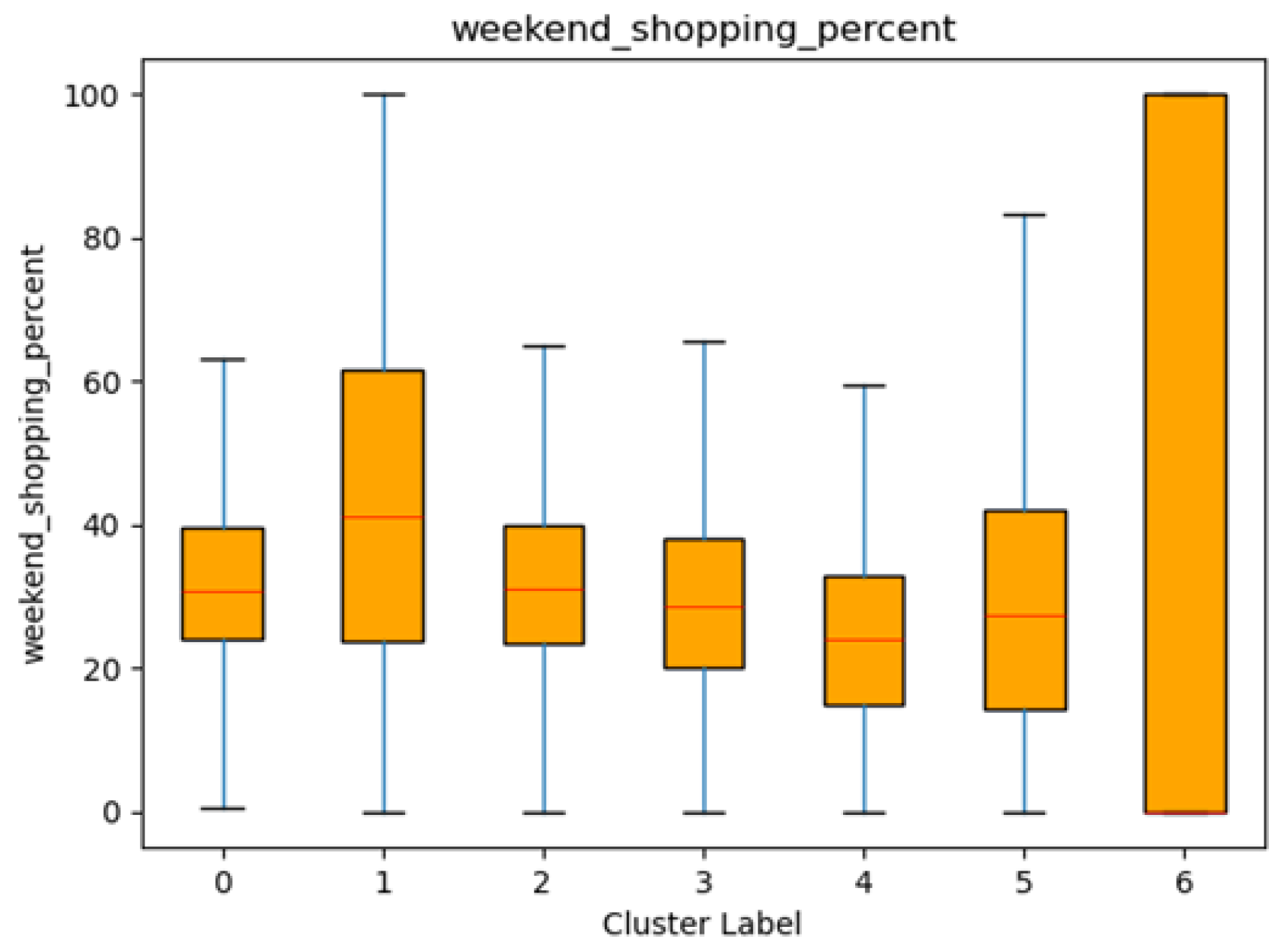
3.7. The Percentage of Shopping on the Weekend

The proportion of shopping conducted on weekends also provides unique insights into customers’ shopping patterns and preferences. By examining the mean, median, and spread of weekend shopping percentages across different customer segments, we can identify segments that are more inclined to make purchases on weekends, as well as those that appear less influenced by weekend shopping opportunities.

In general, Cluster 1 exhibits the highest average proportion of weekend shopping (mean = 43.23%), suggesting that these customers are particularly likely to carry out their shopping on weekends. The median value of 41.23% reinforces the tendency toward weekend purchases within this group, although their standard deviation (25.62) indicates a moderate spread in behaviour. By contrast, Cluster 4 shows the lowest mean percentage (25.09%), implying a preference for weekday shopping. Its median is 24.10%, again underscoring the relatively limited weekend engagement among these consumers. Clusters 0, 2, 3, and 5 display mean weekend shopping proportions ranging from roughly 30% to 33%, indicating moderate weekend shopping activity. Cluster 6 is notable for having a large standard deviation (43.67) and a median of 0.00, suggesting the presence of customers who rarely shop on weekends alongside others with very high weekend shopping percentages. This wide variability points to the heterogeneous nature of shopping behaviour within Cluster 6.

Figure 11. Box plots of the percentage of shopping in the weekend by clusters.

Figure 11. Box plots of the percentage of shopping in the weekend by clusters.

3.8. The Most Frequently Purchased Items

Examining the most frequently purchased items can inform the design of micro-level actions for both customers and retailers (e.g., targeted purchases and promotional strategies). However , due to the large amount of missing data, only 40% of customers could be linked to specific items. We also attempted clustering using only the subset of customers with item-level data, but the results were broadly similar. Consequently, items purchased were not included in the final clustering. Table 2 presents the top 10 most frequently purchased items.

Overall, the rankings remain consistent across most clusters, with the same 10 items—beverage, chips, juice, cheese, butter, mayonnaise, eggs, yogurt, milk, and sugar—appearing most often. Two exceptions are Cluster 1 and Cluster 6. As mentioned above, Cluster 6 mostly comprises of one-time shoppers, leading to a different ranking; milk and sugar are replaced by bread and cereals. In Cluster 1, cereals replace sugar, while the remaining items appear in similar positions as in other clusters.

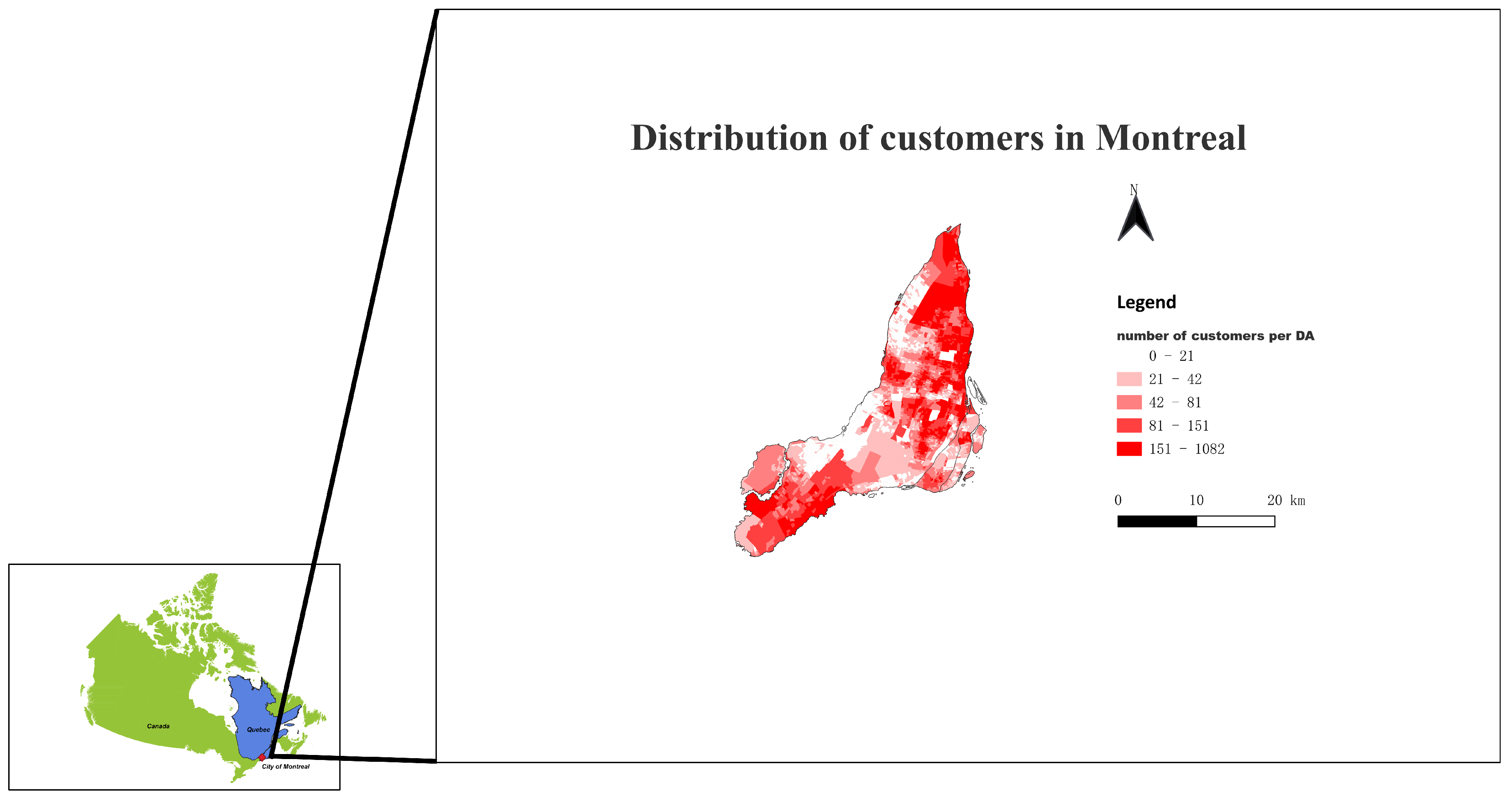
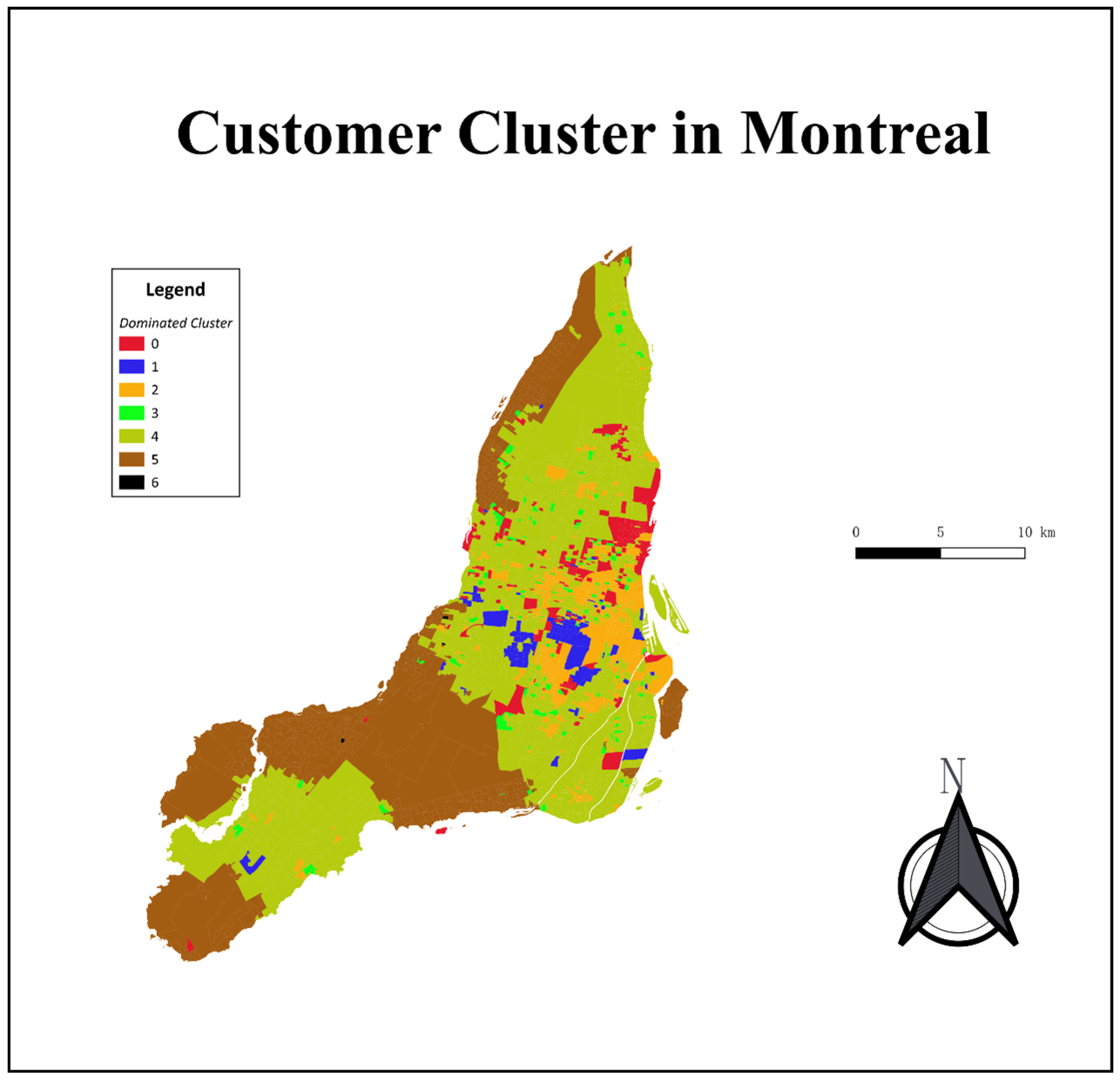
3.9. The Spatial Distribution of Customer Clusters

Understanding how customer segments are dispersed across a city can offer valuable insight into localized consumer behaviour, potentially guiding marketing strategies, resource allocation, service planning, and further aiding ABM modelling. Figure 12 illustrates the spatial distribution of the seven identified customer clusters in Montreal, which is similar to a presentation of geodemographics [14]. Each color-coded region represents the dominant cluster in that area, allowing for a clear visualization of where each segment is most prevalent. The basic spatial unit is dissemination area (DA), which is the smallest standard geographical unit in Canadian census available to the public.

As shown in Figure 12, Clusters 4 and 5 dominate much of the total region, although they occupy distinct areas. Cluster 4, the most populous cluster, is concentrated in central and eastern Montreal, as well as in southwestern suburbs. By contrast, Cluster 5 primarily appears in suburban areas, especially those located far from retail stores, though it comprises fewer individuals overall. Meanwhile, Clusters 0, 1, and 2 cluster around the downtown core, where they are largely surrounded by Cluster 4. In addition, Clusters 3 and 6 are the least populous, and thus only a small number of DAs are dominated by these segments.

To further understand the spatial contiguity, we also compute the overall join count ratio of this landscape with rgeoda library [23], since some widely used metrics, such as Moran’s I, are not suitable for the categorical variable with multiple classes[8]. The overall join count ratio is 0.6793, which means 67.93% of total connections among adjacent objects belong to the same cluster [19], and this indicates a moderate to strong tendency of spatial clustering.

4. Conclusion and Discussion

In this study, seven distinct customer segments were identified using both demographic and behavioural attributes. Each cluster exhibits unique characteristics that can inform targeted marketing strategies, store location planning, and personalized promotions. Table 3 summarizes each segment and provides a descriptive label that captures its principal shopping profile. For example, Cluster 4’s label of “Weekday Day Shoppers” represents the average shopping behaviour for the majority of customers. They usually shop at a nearby store, and prefer to shop on weekdays and in the daytime. This clearly distinguishes them from other clusters. For example, cluster 0 represents the most “Frequent Store Explorers”; they visit the retail chain’s stores on a weekly basis and frequent multiple locations, suggesting variety-seeking and convenience-oriented habits. Cluster 1, “High-Spending Weekend Shoppers”, have a lower shopping frequency but highest spending per trip, and they strongly favor weekend shopping. Individuals belonging to Cluster 2 usually shop at evening, and nearby their residences. While people in Cluster 3 have the highest income, their behaviour is quite similar with Cluster 0, yet they have a lower shopping frequency and travel further to get to stores. Cluster 5 represents those who travel far and are infrequent customers, and they also spend moderately. This may result from their shopping in stores under different brands, and this also possibly explains the behaviours of Cluster 6. Cluster 6 appears to be a group of outliers, as its members only shop at the chain’s stores intermittently over a three-year period, suggesting they may rely on other shopping options, have relocated outside the study area, or took the membership for a one-off access to promotional pricing.

Segmentation results like this not only enhance the understanding of the local customer landscape, but can also support targeted marketing strategies, and inform store location planning. Retailers could leverage the findings to refine store placement in areas with dense clusters of high-value or frequent shoppers. Further, they might tailor promotions by linking them to known cluster preferences in the neighbourhood area, as indicated by the mapping of clusters in Figure 12. For instance, store managers in the downtown core area can hold weekend and after-work promotions and deals for Cluster 1 and Cluster 2, since they are concentrated in that region.

Policy makers and urban planners can also utilize this study to understand how demographics and distances interact with shopping frequency, which may guide further infrastructure development or store location decisions. For example, although it is possible that Cluster 5, who live in suburban areas, have shopping alternatives in their surroundings, improving infrastructure and establishing new stores in that region will decrease travel distance, and possibly cause them to shift to Cluster 0-4, thereby further increasing the engagement of these consumers.

Agent modellers also benefit from these insights. They can draw on these findings to capture both the quantitative behaviour of consumers and the heterogeneity represented by the clusters. Additionally, the spatial distribution of these clusters can inform model initialization, and enhance the realism of more precise and robust simulations intended to reflect actual consumer landscapes.

However, several limitations and uncertainties should be noted. First, the reliance on loyalty program data means that only registered members could be analyzed, thereby excluding those who opt out of such programs. Further, there are also uncertainties within the loyalty dataset [24], such as the outliers in Cluster 6 (some of whom may have joined as a one-off to access promotional pricing). Future research should consider collaborating with multiple retailers or incorporating additional datasets to capture a more representative customer behavior landscape. Second, while the synthetic population provides valuable demographic attributes, its matching process—based on the nearest-neighbor approach—introduces potential spatial uncertainty, especially in densely populated areas. To minimize the impacts of this, we only incorporate income, an attribute that has been shown to have distinct spatial distribution across Montreal, and important to the action of purchase. Third, raw data quality also limits our choice of clustering attributes, for example, missing records of items purchased. In future work, incorporating other sources of data could help to generate greater insights at the micro-level.

In summary, this study demonstrates that merging loyalty program transactions with synthetic population can yield quantitative and spatially explicit insights into the multifaceted nature of grocery-shopping behaviours. Distinguishing customers into seven segments reveals substantial diversity in the dimension of spatial distribution, shopping behaviours, and demographics. These insights, in turn, can guide data-driven interventions—ranging from marketing campaigns to store location optimizations and urban planning initiatives—to better address the needs of Montreal’s diverse consumer base. Ultimately, this approach provides the basis for ABM approach that can enhance our capacity to plan more effectively for the dynamic interplay between customers, retailers, and the broader spatial environment in which these actors operate.