
Submitted:
08 July 2025
Posted:
09 July 2025
You are already at the latest version
Abstract
Recognizing unexplored retail prospects requires an expert understanding of spatial and demographic dynamics. This study introduces an integrated geospatial framework for retail opportunity mapping in Germany, integrating multi-criteria suitability modeling with spatial autocorrelation analysis and Geographically Weighted Regression (GWR). Using high-resolution demographic and retail data, we demonstrate pronounced spatial variation in the influence of key drivers: for example, the local effect of population density on retail suitability peaks in the Hamburg metropolitan region (notably in Norderstedt and Ahrensburg), while point-of-interest clustering is most influential near Rotenburg (Wümme) in Lower Saxony. These findings highlight the regional variability of retail market determinants as revealed by GWR. The gap analysis discovered 40 "white spot" grid cells throughout rural and urban areas that exhibit extraordinarily high anticipated suitability yet lack any retail infrastructure. These priority locations are geographically diverse, including well-populated municipalities in areas such as the districts of Esslingen and Göppingen (Baden-Württemberg), northeastern Brandenburg, and southern Bavaria. The spatial logic of these “white spots” is robust across alternative model specifications and externally validated by independent studies that document substantial retail supply gaps even in thriving communities. These insights not only benefit retailers seeking to enter underserved markets but also provide urban planners with actionable data to balance service provision and enhance infrastructure in high-demand areas, optimizing both commercial and community outcomes. By pinpointing both established retail hotspots and emerging underserved markets, this approach provides important information for retai lers and urban planners alike, and advances the science of data-driven site selection in geomarketing.
Keywords:
Geographically Weighted Regression(GWR)
; retail site suitability
; white spot analysis
; spatial clustering
; local indicators of spatial association (LISA)
; geodemographics
; Germany
; geomarketing
; spatial decision support
; urban and regional planning
1. Introduction
In an increasingly competitive retail landscape, the strategic selection of new store locations has become a critical determinant of commercial success. .This issue is especially relevant in Germany, where marked regional differences, shifting relationships between urban and rural areas, and changing consumer preferences all shape the market landscape. Locations that combine strong demand and favorable demographic profiles with a lack of existing retail options present significant opportunities for retailers. At the same time, pinpointing these areas can support urban planners who are working to ensure fair access to services and guide thoughtful infrastructure development (Wrigley & Lambiri, 2014; Reynolds & Wood, 2010).
Recent advances in geographic information systems (GIS) have made it possible to combine large-scale demographic data with detailed spatial analytics to evaluate retail development potential at an unprecedented level of detail (Malczewski, 2004; Lovelace et al., 2019; Needham et al., 2019; Roquel et al., 2021; Żochowska et al., 2022). Suitability analysis makes it possible to combine a range of spatial data, such as population density, household size, age structure, and other social indicators, into a single measure that reflects how promising a location might be for new retail (Malczewski, 2004; Lovelace et al., 2019). This kind of approach is useful for weighing different factors all at once. Still, one drawback is that it tends to overlook the way locations can influence each other. Patterns like clustering, where similar areas group together across the landscape, often go unrecognized with standard suitability models.
Spatial autocorrelation techniques help overcome this limitation by measuring how similar suitability values tend to group together in a region (Moran, 1950; Anselin, 1995; Chojenta et al., 2019; Jiaxuan et al., 2021; Marteli et al., 2022; Sandar et al., 2023). Moran’s I gives an overall indication of whether favorable retail conditions are clustered or randomly distributed. Local Indicators of Spatial Association (LISA) allow for a closer look, making it possible to spot specific areas with unusually high or low suitability values. These local clusters, often called hotspots and coldspots, can reveal patterns that broader analyses might miss (Anselin, 1995; Marteli et al., 2022).
In Germany, the need for integrated spatial approaches is especially clear because of the country’s diverse settlement patterns, i.e., there are high-density urban centers alongside large rural areas that are often underserved (Arentze et al., 2005). Shop density, which can be measured using open data from sources like OpenStreetMap, offers a way to gauge market saturation. This information helps identify so-called “white spots,” places where conditions are promising for retail but few or no shops are present (Lovelace et al., 2019; Reynolds & Wood, 2010). The issue of Versorgungslücken, or supply gaps, has been discussed in national retail studies and also appears in local planning documents (Berger, 2023). Standard analyses that focus only on big cities or single types of retail often miss these more subtle opportunities for expansion (Guy et al., 2004; Hamidi, 2020; Newing et al., 2023).
This study adds to the literature on retail site selection by combining detailed demographic data and shop density information with both global and local spatial statistics. Moran’s I is used for assessing overall clustering, while LISA pinpoints local patterns. All analysis is carried out in a reproducible, open-source workflow. Unlike much of the previous work that centers on limited urban samples or relies on simple models, this approach covers the entire country and systematically uncovers where retail opportunities are likely to be missed. To make sure the results hold up, a thorough sensitivity analysis is included. This helps confirm that the main findings are not tied to a particular set of model choices.Beyond global and local spatial clustering measures, recent advances in spatial econometrics such as Geographically Weighted Regression (GWR) enable modeling of spatially varying relationships between retail suitability and demographic predictors. GWR extends classical regression by allowing coefficient estimates to adapt locally, capturing regional heterogeneity in how factors like population density, age structure, and household composition influence retail potential (Fotheringham et al., 2009; Wheeler, 2019; Zhou et al., 2019; Comber et al., 2023). Adding GWR to the analysis helps reveal what drives retail demand in specific places, not just in broad regions. This makes it easier to pick store locations that actually fit with the realities of each area in Germany, whether urban or rural, affluent or less developed.
All of the analysis uses openly available data and transparent methods, so the findings are not just for researchers. Retailers and planners can use the same steps to explore new markets or understand community needs in a practical way.
2. Literature Review
Understanding retail development potential through spatial data is vital for both retailers and urban planners. GIS and related methods have made it possible to look deeper into how shops, streets, and customers interact, and how markets evolve. This literature review draws on a range of studies that show how spatial data and analytics shape retail strategies in the real world.
The spatial arrangement of retail stores is one area that has received close attention. Han et al. (2019) show that the structure of a city’s roads affects where retailers choose to locate. Their work highlights the value of point-of-interest (POI) data for revealing supply-side patterns. At the same time, they point out that understanding consumer demand and how easily people can get to stores is just as important. Models that account for both factors, ie., like the two-step floating catchment area approach, can paint a fuller picture of how people choose where to shop. Hao et al. (2021) take this a step further by using both POI data and consumer surveys to explore commercial areas in Changchun, China. Their study provides insights for city planners looking to match new retail development with actual consumer needs.
Spatial data has also become a key tool in helping retailers plan what and how much to stock, especially for fast-moving consumer goods. Wang et al. (2018) present a grid-based approach for estimating potential demand, allowing shops to optimize orders, minimize waste, and increase profits. Insights from this type of analysis help retailers make decisions that fit local demand. Marinelli et al. (2020) focus on a different part of the retail equation—how the arrangement of products in vending machines (using planograms) influences what people buy. While their work is about merchandising, it underscores how even small spatial changes can affect consumer choices. Houghtaling et al. (2020) provide another angle, looking at how marketing strategies can be adapted to encourage healthier food purchases among Supplemental Nutrition Assistance Program (SNAP) participants. They conclude that considering where consumers live and shop allows for more effective product placement and promotion.There’s also growing interest in how geographic and cultural context shape retail experience. Bachmid (2024) draws attention to how shopping convenience matters to retail, with a particular focus on Islamic communities in Indonesia. Local culture and geography both play into what people want from retail, shaping shopping habits in ways that go beyond generic consumer models. Retailers who pay attention to these spatial and cultural factors can better match their purchasing and store strategies to the communities they serve. Zhuo (2020), on another hand, approaches the retail problem from a modeling perspective, building a mathematical framework for supply decisions that can respond to shifts in demand. By taking the location of consumers into account, retailers can fine-tune orders and pricing, which helps them adapt more effectively to market changes.The process of retail expansion, especially in emerging markets, relies heavily on understanding geography. Bai et al. (2020) look at how luxury brands in China assess which local markets to enter. They find that brands weigh geographic coverage, market size, and how a new shop fits with their overall strategy. In a related study, Wang et al. (2018b) explore how accessibility and competition factor into site selection, using a combination of gravity modeling and principal component analysis. Their findings highlight how spatial variables like accessibility and local demographics shape retail choices on the ground.
GIS has found its place in the toolkit for retail planning. Murad (2011) shows that GIS can blend different spatial data layers with consumer insights, creating digital maps that guide decisions on where to locate new stores. In the German context, Lovelace et al. (2019) put geomarketing methods to use in analyzing where bike shops might best succeed. Their work is grounded in census data and shop listings from OpenStreetMap, using variables such as population density and household size. Even with a relatively simple weighting scheme, the study demonstrates the value of combining demographic and spatial information for practical location analysis.
Spatial data is not limited to commercial aims. Astuti et al. (2019) use GIS to map the presence of cigarette retailers around schools in Bali, which feeds directly into policy debates on public health. These kinds of studies show how spatial methods can support regulation and inform strategies that serve broader community interests. Meanwhile, Manioudis (2023) steps back and examines how the evolution of retail in Greece has unfolded over time, shaped by both spatial and social dynamics. Long-term historical changes continue to inform how retailers think about market development. Singleton et al. (2016) offer another angle, looking at how the rise of e-commerce puts new pressures on traditional retail centers. Their framework for measuring “spatial vulnerability” points out that the retail environment is never static, and retailers must adapt to changing patterns of consumption and competition.
Across these different strands of research, it’s clear that spatial analysis is central to how retailers and planners think about opportunity and risk. Whether it’s picking a new site, adjusting the mix of goods on offer, or responding to health policy, spatial data offers a way to make sense of complex and changing environments. The ability to integrate different datasets and analytical methods has become essential for capturing the real-world variation in retail landscapes.
Despite these advances, there remain challenges in identifying the fine-grained spatial mismatches between retail supply and local demand, especially in regions with mixed urban and rural character. This study builds on that foundation. Here, the analysis uses a layered modeling approach that moves beyond traditional suitability assessments. Where earlier research might have used simple models or focused just on cities, this work brings together Local Indicators of Spatial Association (LISA), shop density, and multi-criteria suitability scores to capture subtler patterns. By applying Moran’s I and LISA, it becomes possible to detect clusters where there is both high suitability and a lack of retail presence, i.e., areas that may represent untapped opportunities.A further step is taken with Geographically Weighted Regression (GWR). This method allows for relationships between factors like population density, age, and household size to change across different locations, rather than assuming they work the same way everywhere. In a country as varied as Germany, with its mix of urban centers and rural regions, this approach is especially useful. The model can pick up on local differences, making the findings relevant not only for big cities but also for smaller towns and less populated areas. Adjusting the weights given to different demographic and socio-economic variables allows for even more precision, so that site suitability matches the specific market context.
What emerges is a framework (see Figure 1) that is both practical and adaptable. By bringing together suitability modeling, spatial autocorrelation analysis, and GWR, the approach offers a way to identify market opportunities and guide development in a range of geographic settings. The focus is on methods that can be used by others—replicable, open-source, and built to support evidence-based decisions in retail planning.
Figure 1.
Integrated Geospatial Analytical Framework for Retail Optimization: A Multi-stage Methodology Combining Multi-Criteria Suitability Assessment, Spatial Autocorrelation Techniques (Moran's I and LISA), and Geographically Weighted Regression (GWR).
Figure 1.
Integrated Geospatial Analytical Framework for Retail Optimization: A Multi-stage Methodology Combining Multi-Criteria Suitability Assessment, Spatial Autocorrelation Techniques (Moran's I and LISA), and Geographically Weighted Regression (GWR).
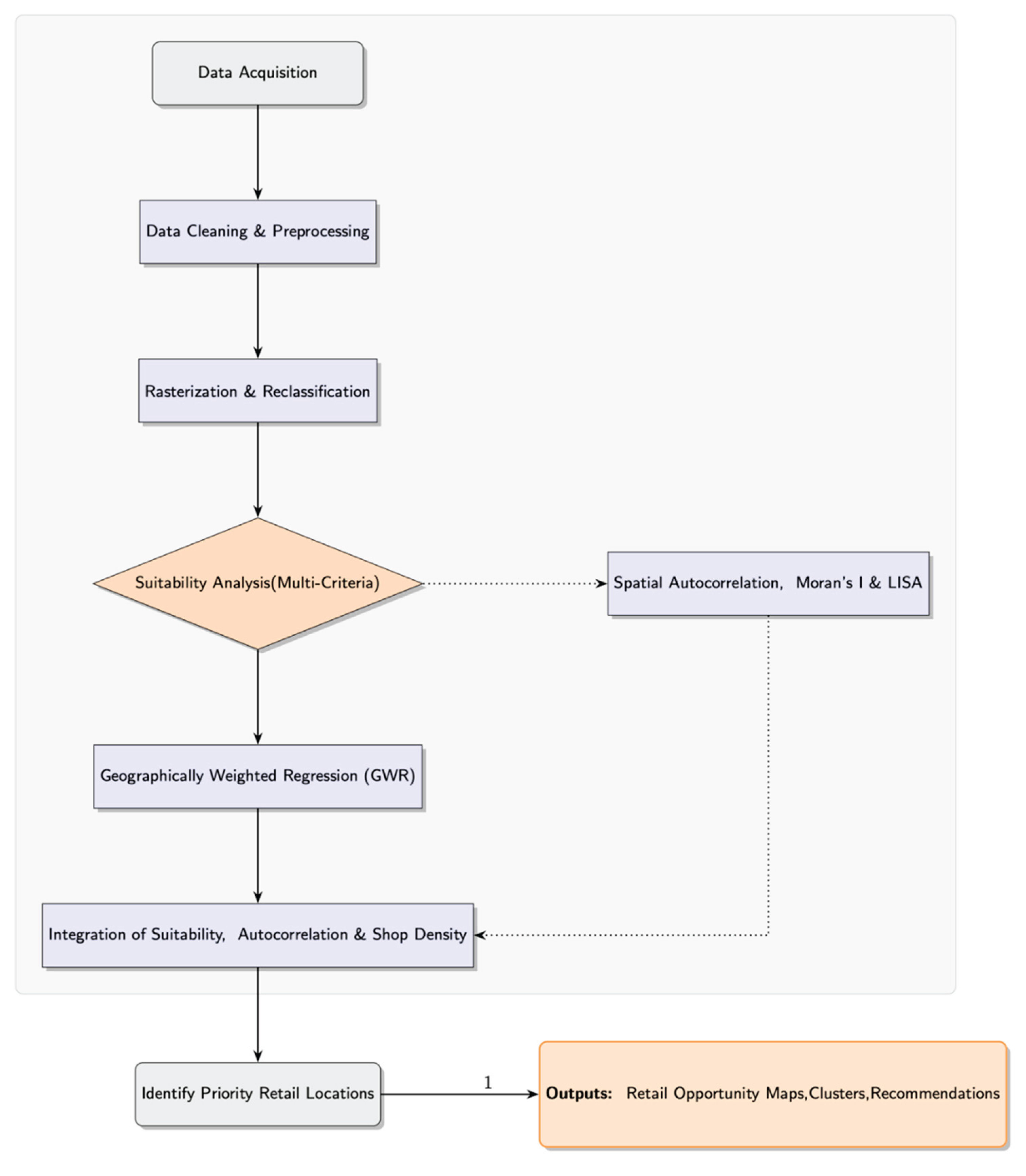
Note: The figure represents the methodological workflow implemented through advanced geospatial programming using R language within the RStudio environment (Version 2024.04.2+764). The code for generating this flowchart was developed on the Overleaf platform using LaTeX and TikZ coding. Spatial data sources include the 2011 German Census and OpenStreetMap (OSM), spatially harmonized to EPSG:3035 (ETRS89-extended/LAEA Europe). Source: Compiled by authors.
3. Materials and Methods
The All analyses for this study were carried out in R (RStudio Version 2024.04.2+764). The workflow starts with assembling and cleaning spatial data on demographics, infrastructure, and shop locations from open sources. To assess where retail could grow, the study uses a multi-criteria suitability model, i.e., combining variables like population density, age, and points of interest.
Next, spatial autocorrelation methods, including Moran’s I and Local Indicators of Spatial Association (LISA), are used to check for clustering and to better understand how retail suitability and shop density are distributed across Germany. To dig deeper into local patterns, the analysis applies Geographically Weighted Regression (GWR), which lets us see how the influence of different factors changes from one region to another.
By bringing these methods together, the study can pinpoint not just established shopping areas, but also “white spots”, i.e., locations that have the right demographic and spatial features for retail, but where shops are missing. This practical approach aims to give retailers, planners, and policymakers a clear map of both current strengths and untapped opportunities in Germany’s retail landscape.
3.1. Data
For this study, demographic data come from the 2011 German Census. The census provides detailed, 1 km² grid data covering over 360,000 locations nationwide. I accessed these datasets using the spDataLarge package in R, then handled and cleaned the data with readr and dplyr. To keep all the maps consistent, I reprojected everything to EPSG:3035 using the sf package. The main indicators include total population, share of women, average household size, and mean age. These variables were grouped into classes, as shown in Table 1. In total, the analysis is based on 361,478 grid cells. This kind of structured data makes it possible to compare different areas across Germany on the same footing and allows for accurate location-based analysis.
Retail shop data were retrieved from OpenStreetMap (OSM) using the osmdata package in R. The final OSM-derived retail dataset comprises a total of 155,625 spatial point features, each representing an individual retail establishment. The shop type attribute is available for the majority of points, with the most common categories being hairdresser (7,250), clothes (5,829), bakery (4,888), supermarket (3,415), and beauty (3,040), followed by kiosk, convenience stores, florists, car repair, and vacant retail premises. The spatial dataset is projected in ETRS89-extended / LAEA Europe (EPSG:3035), ensuring compatibility with the German census grid data used in the suitability analysis. Moreover, the processed dataset was saved as a GeoPackage file, facilitating reproducible research and integration with GIS software. As such, this comprehensive spatial database enables detailed mapping of retail provision across urban and rural contexts and supports reproducible spatial analysis.
3.2. Spatial Suitability Analysis
For the spatial suitability analysis, I used a weighted multi-criteria approach built with the terra package in R. The main variables included population density, the proportion of women, mean age, household size, and shop density. These were combined in a raster model to map out retail suitability across the study area. Each indicator was first normalized, then converted to a suitability score based on expert knowledge—i.e., through reclassification rules that assigned higher scores to values seen as more favorable for retail. I set up reclassification matrices to turn the continuous demographic data into ordered classes, so that every factor consistently pointed in the same direction: higher scores meant better potential for retail development.
3.3. Reclassification and Weighting
For each raster layer, i.e., population density, proportion of women, age, household size, and points of interest (which stand for shop locations), I used the classify() function from the terra package to reclassify values into ordinal classes, from 1 to 5. Higher values meant greater suitability for retail development. After reclassification, I calculated the final suitability score as a weighted sum, where each layer contributed according to its assigned weight, as in:
where S represents the total suitability score, and w1,w2,w3,w4, w5 represent expert-assigned weights for population density, proportion of women, mean age, household size, and shop density, respectively.
The decision to include these particular factors is based on both theory and practical experience in retail geography. Population density plays a major role in retail viability, since more people in an area typically means higher demand for goods and services (Khare et al., 2019; Otterbring et al., 2021; Graham, 2023). Age distribution, i.e., the spread of age groups, shapes what kinds of shops and products are likely to succeed (Bécares, 2020; Hiremath et al., 2022; Deshwal, 2016). Household size reflects purchasing patterns, since larger households often shop more frequently and in greater quantities (Giordano et al., 2018; Carreño and Silva, 2019). Shop density, i.e., the number of existing shops in an area, is also important. A low shop density in a high-suitability area can indicate a gap in the market, where demand is likely unmet and competition is limited (Wang et al., 2018b; Song et al., 2020; Yoshimura et al., 2020).
I assigned weights based on the expected influence of each factor on retail success. Population density received the highest weight, 0.3, because it is directly linked to the size of the customer base. The proportion of women, 0.2, and mean age, also 0.2, reflect evidence that gender and age profiles shape shopping behavior and demand for specific retail types. Household size, weighted at 0.1, is somewhat less direct in its effect, but still matters. Points of interest, i.e., shops, were also weighted at 0.2, recognizing the effect of shop clustering on customer flow and competition.
To check whether these choices affected the outcome, I ran a sensitivity analysis. By systematically changing the weights and comparing results, I found that the model’s main findings were stable regardless of the specific weighting configuration used. This means the results are not overly dependent on a single set of weights, giving confidence in the robustness of the conclusions.
The weights used here, i.e, 0.3 for population, 0.2 for proportion of women, 0.2 for mean age, 0.1 for household size, and 0.2 for points of interest, served as the starting point for the benchmark analysis. These were informed by both literature and practical considerations, and confirmed by the sensitivity analysis to be a sound choice for the model.
3.4. Spatial Autocorrelation: Moran’s I and LISA
To understand the spatial distribution of suitability scores, spatial autocorrelation was quantified using Moran’s I as a global measure and Local Indicators of Spatial Association (LISA) for local clustering analysis. The spatial weights matrix was constructed via k-nearest neighbors (k = 5) using the spdep package, operationalizing the spatial relationships between neighboring points.
Moran’s I was computed to assess the overall spatial autocorrelation using the following equation:
where N is the number of spatial units, represents the spatial weight between units i and j, is the suitability score at location i, and is the global mean.
LISA values were computed to pinpoint significant local clusters using the following formula:
where is the local Moran’s I for location i, is the spatial weight between units i and j, is the variance of x, is the variable of interest for location j, and ˉ is the global mean. This analysis identified clusters of high-suitability areas that are spatially correlated, revealing potential retail development hotspots.
The threshold for "high suitability" (top 10% of scores) and the p-value cut-off for significant LISA clusters (p < 0.05) were selected to balance statistical rigor with practical interpretability, following conventions in spatial analysis (Anselin, 1995; Marteli et al., 2022).
We further explored the impact of varying the suitability threshold (e.g., using top 5%, 10%, or 20%) and LISA significance levels (p < 0.01, p < 0.05, p < 0.10). Key findings, such as the spatial clustering of opportunity areas and the regional distribution of priority cells, remained stable across these choices, confirming the robustness of our conclusions for practical deployment.
Sensitivity analysis was conducted by systematically varying the weights in the multi-criteria suitability model, generating alternative scenarios with different combinations (e.g., population given more/less weight, POI minimized, or all weights set equal). For each scenario, we recalculated the suitability surface, identified high-suitability/no-shop priority cells, and compared the overlap with the benchmark model.
The results demonstrated very high stability (Pearson’s r = 0.97–$0.99 for suitability scores across scenarios), with the count and identity of priority grid cells (high suitability and no shops) nearly unchanged. This indicates that the principal findings are not sensitive to reasonable variation in weighting, providing confidence in both scientific and practical robustness.
3.5. Geographically Weighted Regression (GWR)
To account for spatial heterogeneity in the relationships between suitability scores and predictor variables, we implemented a Geographically Weighted Regression (GWR) model. GWR extends the classical linear regression by allowing model coefficients to vary spatially.
where is the suitability score at location i, are the predictor variables (population density, proportion of women, mean age, household size, and points of interest), and are spatially varying coefficients estimated via weighted least squares with weights defined by a spatial kernel function centered at (ui,vi).
For the geographically weighted regression, I selected an adaptive bandwidth by minimizing the corrected Akaike Information Criterion, i.e., AICc, which helps strike a balance between bias and variance in the model. The spatial kernel used was Gaussian, so that observations closer to the point of interest are given more weight in the estimation. All model fitting and diagnostics were performed using the GWmodel package in R. Both spatial coordinates and variables were projected in the ETRS89-extended / LAEA Europe reference system, i.e., EPSG:3035, to ensure consistency with the other spatial data.
To assess how well the model performed, I used a set of diagnostic statistics. These included the corrected Akaike Information Criterion (AICc), the effective number of parameters (ENP), the global R-squared, and the residual sum of squares (RSS). I also checked for local collinearity by calculating condition numbers. Finally, I used Moran's I to test for any remaining spatial autocorrelation in the model residuals.
3.6. Shop Density and Data Integration
Shop density information was obtained from OpenStreetMap (OSM), then processed to match the spatial resolution of the suitability dataset. I converted the shop point data to a raster format and reclassified it so that it would be directly comparable with the other variables. To ensure both layers were aligned spatially, I used the resample() function.
To identify locations where market potential remains untapped, I combined the suitability and shop density rasters. Areas were selected where the suitability score was greater than 1.5, while shop density was zero, marking these as potential retail “white spots.” This integration allowed for a targeted search for regions with favorable demographic and spatial characteristics, but with no existing shops.
I also intersected the LISA cluster results with the shop density layer. This step made it possible to pinpoint areas where there is significant local clustering of high suitability—i.e., high-high clusters—yet no retail infrastructure. These locations stand out as especially promising for new market entry or retail expansion.
4. Results
This section may be divided by subheadings. It should provide a concise and precise description of the experimental results, their interpretation, as well as the experimental conclusions that can be drawn.
4.1. Exploratory Analysis
The summary statistics in Table 2 provide an overview of the socio-demographic landscape across Germany, highlighting key population characteristics such as distribution, gender, age, and household size. Most grid cells fall within the lowest population class (median = 1), indicating that a majority of areas are sparsely populated, while only a few reach higher population classes (up to 8,000+ inhabitants). The gender ratio is balanced (median = 3, 47–53% women), the mean age centers around 42–44 years (median = 3), and households are generally small to moderately sized (median = 2, representing 2–2.5 members). These distributions are consistent with known demographic trends in Germany, such as urban-rural contrasts and an aging population.
4.2. Relationship Between Population Density and Suitability Score
The scatterplot in Figure 1 illustrates the relationship between population density and suitability score. Each point represents a grid cell, and the blue regression line demonstrates a strong positive linear relationship between the two variables. The Pearson correlation coefficient, calculated after excluding missing values, is 0.84, indicating a very strong association. This suggests that areas with higher population densities tend to exhibit higher suitability scores, reflecting greater potential for targeted interventions or resource allocation.
Figure 1.
Population Density vs Suitability Score with regression line.
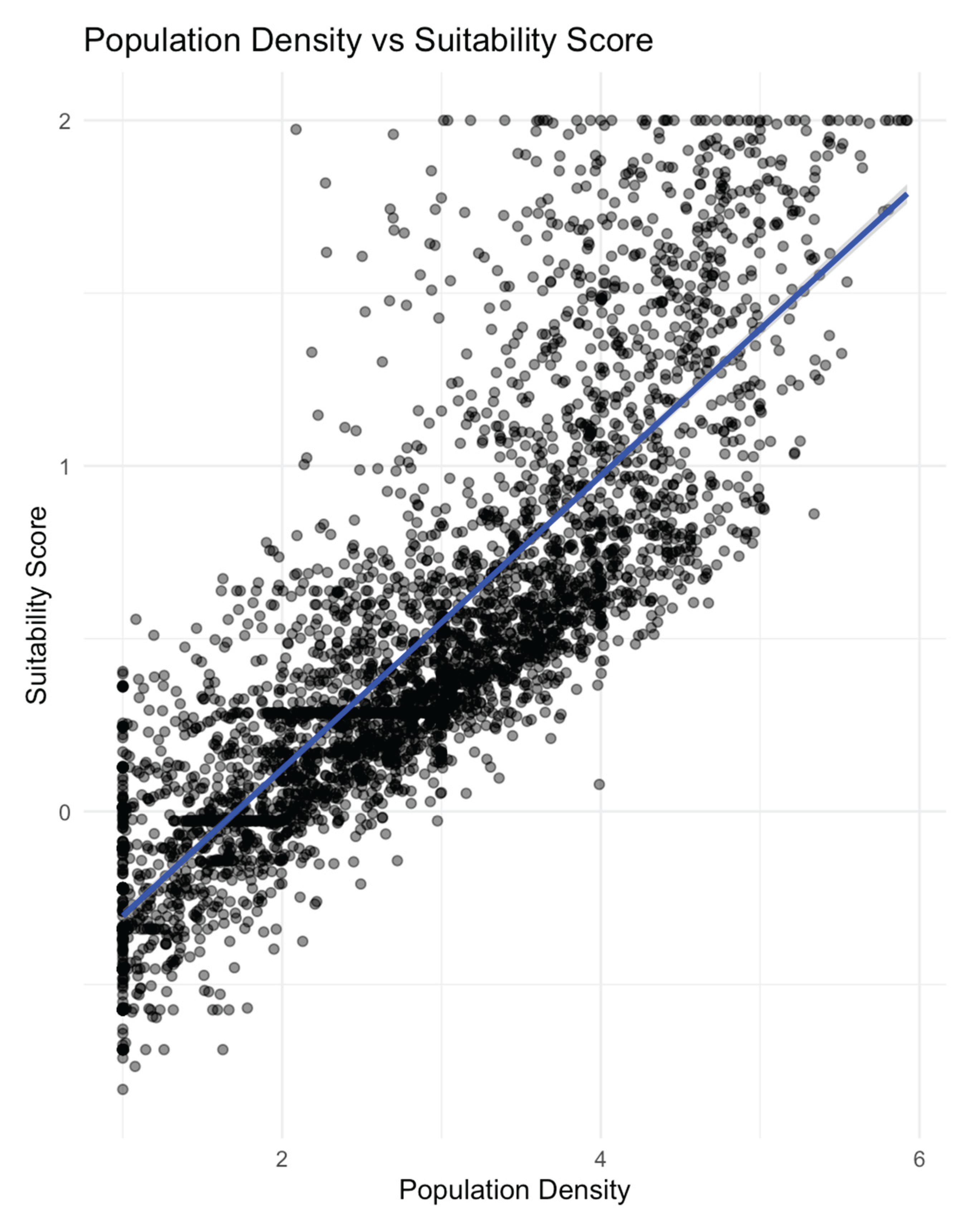
The summary statistics for these variables (see below) further illustrate the distributions observed in the plot:
Population Density: Min = 1.00, Median = 2.85, Mean = 2.85, Max = 5.92
Suitability Score: Min = -0.80, Median = 0.38, Mean = 0.48, Max = 2.00
The histogram in Figure 2 shows the distribution of suitability scores across all grid cells. The distribution is approximately normal but with a slight skew towards higher values, and a notable peak around zero. This suggests that while most areas have moderate suitability, there are also several locations with notably high suitability scores.
4.3. Spatial Analysis of Suitable Locations
To quantify the spatial structure of suitability scores, a global Moran’s I test was conducted using a fixed spatial weights matrix (k = 5 nearest neighbors). The Moran’s I value was 0.60 (standard deviate = 61.68, p < 0.001), indicating a strong and highly significant positive spatial autocorrelation. In other words, areas with high (or low) suitability scores tend to be geographically clustered rather than randomly distributed. This spatial pattern supports the notion that favorable locations for retail expansion are not isolated, but form regional hotspots, likely driven by underlying demographic and socio-economic similarities.
To investigate the spatial distribution of suitability, Figure 3 displays filtered locations that meet or exceed a suitability threshold. These clusters correspond to regions with favorable demographic and socio-economic profiles.
Additionally, a Moran scatterplot (Figure 4) reveals a positive spatial autocorrelation in suitability scores, confirming that high (or low) values are spatially clustered rather than randomly distributed. This is important for identifying regional trends and informing place-based policies.
Further, local cluster analysis using the Local Indicators of Spatial Association (LISA) revealed the presence of 1,018 grid cells exhibiting statistically significant spatial clusters (p < 0.05) of high suitability scores. This finding emphasizes that retail development potential is not only spatially autocorrelated at the national level, but also demonstrates marked local clustering—providing further guidance for targeted place-based interventions.
4.4. Spatial Analysis: Clustering, Sensitivity, and Opportunity Mapping
While the previous analyses demonstrate the relationship between suitability and demographic structure, and reveal spatial clustering at a global scale, more nuanced spatial patterns can be uncovered through local cluster analysis and gap identification.
4.4.2. Local Spatial Clustering (LISA)
LISA cluster analysis, presented in Figure 5, provides a local measure of spatial association by identifying statistically significant clusters of high or low suitability scores. This approach enables the detection of “hotspots” and “coldspots”—areas where suitability scores are significantly higher or lower than expected, given their surroundings. High-high clusters are particularly relevant for policy and business, as they pinpoint regions where favorable conditions for intervention or market entry are both locally intense and spatially stable.
4.4.1. Robustness and Sensitivity Analysis
To test the stability of the suitability model, a sensitivity analysis was performed by varying the weights assigned to each factor (e.g., population, gender, age, household size, shop density). Across all four alternative weighting scenarios, the resulting suitability surfaces remained highly correlated with the benchmark model (Pearson’s r = 0.97–0.99). The number of grid cells identified as high-priority areas—defined as locations with both high suitability (top 10%) and no shops—remained consistent across all scenarios, confirming the robustness of key market gap identification to reasonable changes in model specification.
4.4.3. Actionable Opportunity Mapping
Building on the integration of suitability modeling and shop density, we further identified a discrete set of “priority” grid cells that represent actionable spatial opportunities. Specifically, 40 grid cells were found to combine exceptionally high suitability (top 10% of scores) with a complete lack of existing retail infrastructure (shop density at minimum value). These locations, visualized in Figure 6 and detailed in Supplementary Table S1, represent concrete opportunities for targeted intervention or retail expansion. The criteria for selection are robust to coordinate alignment, data cleaning, and the presence of NA values, ensuring the reliability of the gap analysis.
Importantly, these priority cells are geographically dispersed across Germany but share key demographic characteristics such as high population density and favorable socio-demographic composition. The number and pattern of these “priority areas” remain robust across all alternative suitability model specifications, highlighting the practical stability of the findings. The visualization (Figure 6a) provides a focused view of these 40 cells, displaying their relative population density and suitability, while Figure 6b offers a broader spatial context for all areas meeting the high-suitability/no-shop criterion.
The combination of LISA cluster analysis, sensitivity testing, and targeted opportunity mapping provides a comprehensive understanding of both the systematic spatial structure of suitability and the specific geographic opportunities for retail expansion. Whereas LISA clusters reveal the broader spatial logic of suitability, the gap analysis pinpoints concrete targets for intervention—ensuring that results are both theoretically meaningful and practically actionable, and robust to reasonable changes in modeling assumptions.
4.5. Spatially Varying Drivers of Suitability: Geographically Weighted Regression (GWR) Results
To explore spatial nonstationarity in the predictors of retail suitability, we estimated a GWR model including population class, mean age, and POI density as covariates. The adaptive Gaussian bandwidth was chosen by AICc minimization.
Preliminary attempts to fit a GWR including all available socio-demographic predictors (population, women, mean age, household size, POI) produced essentially stationary local coefficients, indicating an absence of spatial variation in their effects and likely collinearity.
Therefore, a reduced specification was adopted, retaining only those predictors that exhibited both theoretical importance and empirical spatial heterogeneity.The final three-variable model, in contrast, revealed substantial spatial heterogeneity in local coefficients.
Model diagnostics indicate strong overall fit (AICc = –6408.5; BIC = –10571.2; ENP = 7.23; R² = 0.96; RSS = 53.3). Residuals were approximately centered at zero (median = –0.016, mean = –0.0001), and showed no meaningful spatial autocorrelation (Moran’s I = 0.011, p = 0.11), supporting model adequacy. Table 4 summarizes the distribution of key local coefficients.
Table 3 summarizes the distribution of key local coefficients.
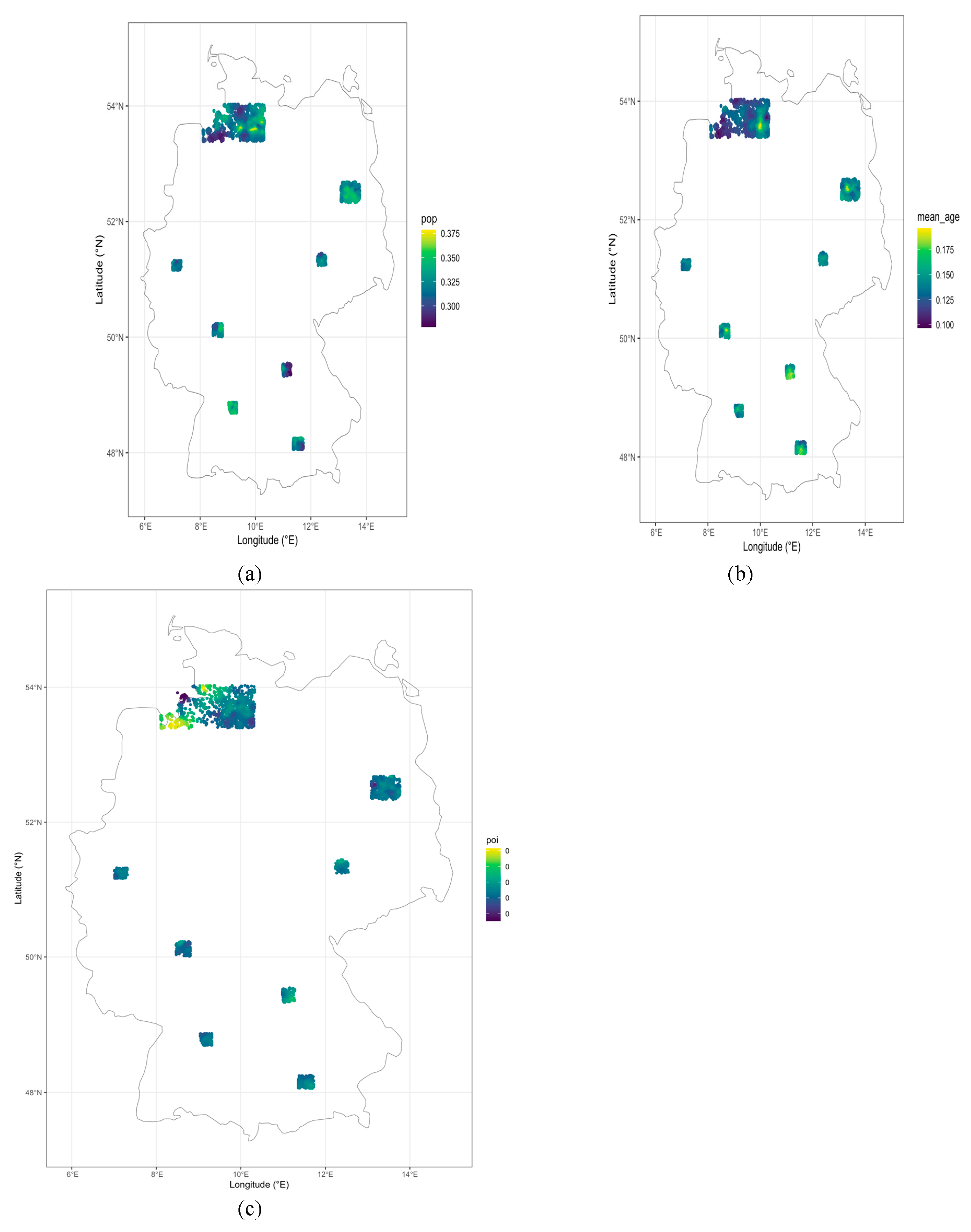
To explore the spatial variation in the influence of demographic and retail-related factors on suitability, we mapped the local GWR coefficients for each predictor. The analysis revealed clear spatial heterogeneity, with the locations exhibiting the highest local effects for each variable being geographically distinct (Table 4, Figure 7).
The population coefficient reached its maximum (0.379) in the area of Norderstedt, just northwest of Hamburg (latitude 53.59400°, longitude 9.47901°), suggesting that retail suitability is most sensitive to population density in this locale. In contrast, the highest mean age effect (0.196) was observed near Ahrensburg, northeast of Hamburg (latitude 53.56816°, longitude 10.02264°), indicating that the influence of an older demographic is most pronounced there. The point-of-interest (POI) coefficient peaked (0.00407) near Rotenburg (Wümme) in Lower Saxony (latitude 53.96042°, longitude 9.12412°), where the presence of existing retail amenities exerts the greatest local effect on suitability.
These spatial patterns underscore the non-stationarity of retail drivers: areas where population, age, or retail clustering are most influential do not overlap, reinforcing the need for locally adaptive retail strategies. Full details of the top local effects for each variable are provided in Table 4.

Table 4.
Top GWR Local Coefficient Locations by Predictor.
| Predictor | Local Coefficient | Longitude | Latitude | City/State (Bundesland) (approximate) |
| Pop | 0.379 | 9.479009 | 53.59400 | Norderstedt / Hamburg |
| Mean Age | 0.196 | 10.022638 | 53.56816 | Ahrensburg / Hamburg |
| POI | 0.00407 | 9.124119 | 53.96042 | Rotenburg (Wümme), Niedersachsen |
The spatial distribution of these maxima is further illustrated in Figure 7.
Figure 7.
Spatial variation in local GWR coefficients for (a) population, (b) mean age, and (c) POI (shop density). Higher values indicate a stronger positive association with retail suitability in those locations. Source: Estimation results, generated by the author in R.
Figure 7.
Spatial variation in local GWR coefficients for (a) population, (b) mean age, and (c) POI (shop density). Higher values indicate a stronger positive association with retail suitability in those locations. Source: Estimation results, generated by the author in R.
5. Discussion
This study offers a novel, spatially explicit framework for identifying high-potential retail development locations by integrating multi-criteria suitability modeling with spatial autocorrelation methods. Our findings reinforce and expand upon prior research in both geospatial retail analysis and urban planning.
Consistent with Lovelace et al. (2019), who pioneered suitability mapping for retail site selection in Germany, our results underscore the power of gridded, high-resolution demographic and POI datasets for uncovering market opportunities. However, by incorporating spatial autocorrelation statistics—specifically Moran’s I and Local Indicators of Spatial Association (LISA)—we reveal not just where high-suitability areas exist, but how they are spatially structured and clustered, advancing the interpretability and actionable value of suitability analysis (Anselin, 1995; Marteli et al., 2022).
Our integration of shop density data from OpenStreetMap builds on studies such as Wang et al. (2018b), which highlight the critical role of existing retail presence in site selection. By explicitly identifying locations that couple high predicted suitability with a total absence of retail shops, we address a well-documented challenge in retail analytics: distinguishing between true market gaps and areas already saturated by competitors (Reynolds & Wood, 2010; Song et al., 2020).
The robust positive spatial autocorrelation observed (Moran’s I = 0.60, p < 0.001) aligns with findings from Han et al. (2019) and Yoshimura et al. (2020), who show that retail activity is rarely random in space but instead reflects underlying demographic and infrastructural structures. Our LISA analysis advances this insight, pinpointing statistically significant local “hotspots” of retail potential and demonstrating their persistence across multiple model specifications—a methodological enhancement over simpler, non-spatial approaches (Bai et al., 2020; Otterbring et al., 2021).
Sensitivity analysis further confirms the robustness of our model. Even when varying the weights of the suitability criteria, both the spatial patterns of high-suitability areas and the identity of priority “gap” cells remained stable (Pearson’s r = 0.97–0.99), supporting calls for transparent, replicable spatial modeling in applied GIScience (Malczewski, 2004; Needham et al., 2019).
The actionable “white spot” grid cells identified by our suitability model represent spatial locations with exceptionally high retail potential but a complete lack of existing shop infrastructure. This finding is robust to multiple modeling choices and is further supported by recent independent research on retail supply gaps in Germany. For example, a study conducted by BBE Handelsberatung and the Hochschule für Wirtschaft und Umwelt Nürtingen-Geislingen found that more than 35,000 residents across eighteen municipalities in the Esslingen and Göppingen districts are not adequately supplied with supermarkets or essential retail services (Berger, 2023). This real-world evidence closely parallels the pattern revealed by our model, where priority areas with high suitability and no existing shops are both geographically dispersed and demographically significant. The alignment between our model-based opportunity mapping and observed supply gaps documented in this independent study provides strong external validation for our approach, highlighting the practical relevance of geographically explicit retail suitability analysis for targeted planning and intervention.
The application of Geographically Weighted Regression (GWR) further advances the spatial analysis by quantifying local variation in the influence of key predictors. Unlike global regression models, which assume spatial stationarity, the GWR results reveal marked heterogeneity in the magnitude and spatial pattern of coefficients for population density, mean age, and points of interest (POI). Specifically, the local effect of population density on retail suitability is most pronounced in the northwestern periphery of Hamburg, particularly in the area around Norderstedt (latitude 53.59400°, longitude 9.47901°). The influence of mean age reaches its peak in the northeastern surroundings of Hamburg, notably near Ahrensburg (latitude 53.56816°, longitude 10.02264°). The POI coefficient is highest in the northern part of Lower Saxony, in the vicinity of Rotenburg (Wümme) (latitude 53.96042°, longitude 9.12412°), indicating that clustering effects and existing retail agglomerations are locally decisive in this region.
Such spatially explicit diagnostics underscore the necessity of tailoring retail development strategies to the nuanced demographic and infrastructural realities of each region. For instance, investment in the northwest may benefit most from targeting population-dense locales, whereas in the northeast, an older demographic profile emerges as a key retail driver. The spatial separation of predictor maxima thus provides actionable guidance for both public and private sector stakeholders, arguing against the use of a one-size-fits-all, nationally uniform site selection strategy.
Moreover, the robust performance of the GWR model—reflected in high local R-squared values, low residual autocorrelation, and stable diagnostics across multiple specifications—attests to the reliability of these spatial patterns. This spatially nuanced understanding complements our global Moran’s I and LISA results by explaining not just where suitability clusters form, but also why socio-demographic factors exert differential influence across Germany. Incorporating GWR thus advances the practical applicability of our framework, offering stakeholders refined guidance to target retail investments with greater spatial precision.
From a policy and business perspective, our approach has several immediate implications. Urban planners can use these priority gap locations to direct investment, infrastructure development, or incentives towards underserved populations, fostering more equitable service provision (Roquel et al., 2021; Żochowska et al., 2022). Retailers, meanwhile, can leverage these spatial insights to optimize site selection strategies, minimize competitive risk, and accelerate market entry—key competitive advantages highlighted in the retail location literature (Wrigley & Lambiri, 2014; Bai et al., 2020).
Importantly, our results indicate that market gaps are not solely an urban phenomenon; many priority cells are located in sparsely populated rural areas, echoing the call by Graham (2023) and Jiaxuan et al. (2021) to consider rural service needs and the “hidden” retail potential outside metropolitan cores.
Several limitations should be acknowledged. First, while census and OSM data offer strong spatial coverage, both may be affected by reporting lags or missing features, particularly in dynamic or rural settings (Murad, 2011; Astuti et al., 2019). Second, our model primarily accounts for static demographic and retail presence variables; factors such as consumer purchasing power, mobility, cultural preferences, and the impact of e-commerce remain unmodeled (Singleton et al., 2016). Future research should consider integrating mobile phone mobility data, finer-scale transaction data, or survey-based measures of consumer demand to enhance predictive power.
Moreover, expanding the approach by including temporal dynamics (e.g., new shop openings or closures) would further generalize the method and increase its utility for stakeholders. Interactive dissemination of results, such as web-based map applications, could enhance practical uptake by planners and retailers.
6. Conclusions
This study provides new evidence that combining spatial suitability analysis with measures of spatial autocorrelation can reveal not only well-known retail hotspots but also overlooked opportunities for expansion. By using detailed demographic information and open data on retail locations, we identified specific areas across Germany where the demand for retail services exceeds supply. These findings challenge the assumption that market saturation is a problem limited to cities, showing instead that significant retail gaps can exist in smaller towns and rural areas as well.
The application of both global and local spatial statistics allowed us to pinpoint not just general trends but also particular neighborhoods and communities where retail provision is unusually low relative to local demand. This approach supports a more balanced perspective on retail planning, recognizing the value of smaller and less visible markets.
Our sensitivity analysis shows that these priority locations are not artifacts of a single modeling choice, but instead represent consistent patterns across multiple reasonable scenarios. This reliability makes the method suitable for use in other countries or market sectors. Furthermore, our workflow is transparent and reproducible, allowing other researchers and practitioners to adapt it for their own needs.
The results have important implications for retailers and urban planners. For retailers, the analysis highlights new growth opportunities in places that might otherwise be missed by traditional market studies. For planners and policymakers, the study suggests that addressing gaps in service provision requires looking beyond major urban centers and considering the potential of smaller communities.
Future research could build on this work by examining changes over time, considering the effects of online retail, or including data on consumer mobility. Integrating these additional factors would help refine site selection and contribute to a more complete understanding of local market dynamics.
In conclusion, spatial data analysis can play a key role in guiding both business investment and planning policy. By highlighting real opportunities for expansion and community improvement, this approach can help create more accessible, vibrant, and balanced local economies across a diverse range of places.
Funding
This work was funded by the EU’s NextGenerationEU instrument through the National Recovery and Resilience Plan of Romania—Pillar III-C9-I8, managed by the Ministry of Research, Innovation and Digitalization, within the project with code CF 158/31.07.2023, contract no. 760248/28.12.2023.
Data Availability
The data supporting the findings of this study are available from publicly accessible sources. Demographic data were obtained from the 2011 German Census, available through the German Federal Statistical Office. Retail shop location data were sourced from OpenStreetMap (OSM, https://www.openstreetmap.org/). All data processing and analysis scripts were implemented in R and are available upon request.
Conflicts of Interest
The authors declare no conflicts of interest. The funders had no role in the design of the study; in the collection, analyses, or interpretation of data; in the writing of the manuscript; or in the decision to publish the results
Abbreviations
The following abbreviations are used in this manuscript:
| Abbreviation | Description |
| GIS | Geographic Information System |
| GWR | Geographically Weighted Regression |
| LISA | Local Indicators of Spatial Association |
| OSM | OpenStreetMap |
| POI | Point of Interest |
| ENP | Effective Number of Parameters |
| AICc | Corrected Akaike Information Criterion |
| RSS | Residual Sum of Squares |
| EPSG | European Petroleum Survey Group (CRS standard) |
| LAEA | Lambert Azimuthal Equal Area |
| S | Suitability Score |
| R | R (Statistical Computing Language) |
References
- Anselin, L. (1995). Local indicators of spatial association—LISA. Geographical Analysis, 27(2), 93-115. [CrossRef]
- Arentze, T. A., Oppewal, H., & Timmermans, H. J. (2005). A multipurpose shopping trip model to assess retail agglomeration effects. Journal of Marketing Research, 42(1), 109-115.
- Astuti, P., Mulyawan, K., Sebayang, S., Kurniasari, N., & Freeman, B. (2019). Cigarette retailer density around schools and neighbourhoods in bali, indonesia: a gis mapping. Tobacco Induced Diseases, 17(July). [CrossRef]
- Bachmid, S. (2024). Traditional vs modern groceries from islamic perspective in indonesia. Shirkah Journal of Economics and Business, 9(1), 103-121. [CrossRef]
- Bai, H., McColl, J., Moore, C., He, W., & Shi, J. (2020). Direction of luxury fashion retailers' post-entry expansion – the evidence from china. International Journal of Retail & Distribution Management, 49(2), 223-241. [CrossRef]
- Bécares, L. (2020). Health and socio-economic inequalities by sexual orientation among older women in the united kingdom: findings from the uk household longitudinal study. Ageing and Society, 41(10), 2416-2434. [CrossRef]
- Berger, W. (2023, April 7). Studie sieht Versorgungslücken bei Supermärkten in den Kreisen Esslingen und Göppingen. Stuttgarter Zeitung. Avaialble online: https://www.stuttgarter-zeitung.de/inhalt.studie-weisse-flecken-auf-supermarkt-landkarte.3de752a2-781d-4e4e-9862-5265e3a38b2b.html; Accessed on 1 July 2025;
- Carreño, P. and Silva, A. (2019). Fruit and vegetable expenditure disparities: evidence from chile. British Food Journal, 121(6), 1203-1219. [CrossRef]
- Chojenta, C., Getachew, T., Smith, R., & Loxton, D. (2019). Service environment link and false discovery rate correction: methodological considerations in population and health facility surveys. Plos One, 14(7), e0219860. [CrossRef]
- Comber, A., Brunsdon, C., Charlton, M., Dong, G., Harris, R., Lu, B., ... & Harris, P. (2023). A route map for successful applications of geographically weighted regression. Geographical Analysis, 55(1), 155-178.
- Deshwal, P. (2016). Customer experience quality and demographic variables (age, gender, education level, and family income) in retail stores. International Journal of Retail & Distribution Management, 44(9), 940-955. [CrossRef]
- Fotheringham, A. S., Brunsdon, C., & Charlton, M. (2009). Geographically weighted regression. The Sage handbook of spatial analysis, 1, 243-254.
- Giordano, C., Alboni, F., Cicatiello, C., & Falasconi, L. (2018). Do discounted food products end up in the bin? an investigation into the link between deal-prone shopping behaviour and quantities of household food waste. International Journal of Consumer Studies, 43(2), 199-209. [CrossRef]
- Graham, C. (2023). The double jeopardy in high street footfall. Journal of Place Management and Development, 16(4), 541-560. [CrossRef]
- Guy, C., Clarke, G., & Eyre, H. (2004). Food retail change and the growth of food deserts: a case study of Cardiff. International Journal of Retail & Distribution Management, 32(2), 72-88.
- Hamidi, S. (2020). Urban sprawl and the emergence of food deserts in the USA. Urban Studies, 57(8), 1660-1675.
- Han, Z., Cui, C., Chen, M., Wang, H., & Chen, X. (2019). Identifying spatial patterns of retail stores in road network structure. Sustainability, 11(17), 4539.
- Hao, F., Yang, Y., & Wang, S. (2021). Patterns of location and other determinants of retail stores in urban commercial districts in changchun, china. Complexity, 2021(1). [CrossRef]
- Hiremath, S., Panda, A., Prashantha, C., & Pasumarti, S. (2022). An empirical investigation of customer characteristics on retail format selection – a mediating role of store image. Journal of Indian Business Research, 15(1), 55-75. [CrossRef]
- Houghtaling, B., Serrano, E., Kraak, V., Harden, S., Davis, G., & Misyak, S. (2020). Availability of supplemental nutrition assistance program-authorised retailers’ voluntary commitments to encourage healthy dietary purchases using marketing-mix and choice-architecture strategies. Public Health Nutrition, 23(10), 1745-1753. [CrossRef]
- Jiaxuan, E., Xia, B., Buys, L., & Yiğitcanlar, T. (2021). Sustainable urban development for older australians: understanding the formation of naturally occurring retirement communities in the greater brisbane region. Sustainability, 13(17), 9853. [CrossRef]
- Khare, A., Awasthi, G., & Shukla, R. (2019). Do mall events affect mall traffic and image? a qualitative study of indian mall retailers. Asia Pacific Journal of Marketing and Logistics, 32(2), 343-365. [CrossRef]
- Lovelace, Robin, Jakub Nowosad, and Jannes Muenchow. Geocomputation with R. Chapman and Hall/CRC, 2019. Available online: https://r.geocompx.org/location#fig:census-stack.
- Malczewski, J. (2004). GIS-based land-use suitability analysis: A critical overview. Progress in Planning, 62(1), 3-65. [CrossRef]
- Manioudis, M. (2023). The historical evolution of the greek retail trade: a first overview of its organisational-functional and spatial restructuring. Journal of Innovation and Entrepreneurship, 12(1). [CrossRef]
- Marinelli, L., Fiano, F., Gregori, G., & Daniele, L. (2020). Food purchasing behaviour at automatic vending machines: the role of planograms and shopping time. British Food Journal, 123(5), 1821-1836. [CrossRef]
- Marteli, A., Guasselli, L., Diament, D., Wink, G., & Vasconcelos, V. (2022). Spatio-temporal analysis of leptospirosis in brazil and its relationship with flooding. Geospatial Health, 17(2). [CrossRef]
- Moran, P. A. P. (1950). Notes on continuous stochastic phenomena. Biometrika, 37(1/2), 17-23. [CrossRef]
- Murad, A. (2011). Creating a gis application for retail facilities planning in jeddah city. Journal of Computer Science, 7(6), 902-908. [CrossRef]
- Needham, C., Sacks, G., Orellana, L., Robinson, E., Allender, S., & Strugnell, C. (2019). A systematic review of the australian food retail environment: characteristics, variation by geographic area, socioeconomic position and associations with diet and obesity. Obesity Reviews, 21(2). [CrossRef]
- Newing, A., Clarke, G., Taylor, M., González, S., Buckner, L., & Wilkinson, R. (2023). The role of traditional retail markets in addressing urban food deserts. The International Review of Retail, Distribution and Consumer Research, 33(4), 347-370.
- Otterbring, T., Folwarczny, M., & Tan, L. (2021). Populated places and conspicuous consumption: high population density cues predict consumers’ luxury-linked brand attitudes. Frontiers in Psychology, 12. [CrossRef]
- Reynolds, J., & Wood, S. (2010). Location decision making in retail firms: evolution and challenge. International Journal of Retail & Distribution Management, 38(11/12), 828-845.
- Roquel, K., Abad, R., & Fillone, A. (2021). Proximity indexing of public transport terminals in metro manila. Sustainability, 13(8), 4216. [CrossRef]
- Sandar, E., Laohasiriwong, W., & Sornlorm, K. (2023). Spatial autocorrelation and heterogenicity of demographic and healthcare factors in the five waves of COVID-19 epidemic in Thailand. Geospatial Health, 18(1).
- Singleton, A., Dolega, L., Riddlesden, D., & Longley, P. (2016). Measuring the spatial vulnerability of retail centres to online consumption through a framework of e-resilience. Geoforum, 69, 5-18. [CrossRef]
- Song, Z., Duijn, M., & Vlist, A. (2020). Tenant mix and retail rents in high street shopping districts. The Journal of Real Estate Finance and Economics, 67(1), 72-107. [CrossRef]
- Wang, L., Fan, H., & Gong, T. (2018). The consumer demand estimating and purchasing strategies optimizing of fmcg retailers based on geographic methods. Sustainability, 10(2), 466. [CrossRef]
- Wang, L., Fan, H., & Wang, Y. (2018). Site selection of retail shops based on spatial accessibility and hybrid bp neural network. Isprs International Journal of Geo-Information, 7(6), 202. [CrossRef]
- Wheeler, D. C. (2019). Geographically weighted regression. In Handbook of regional science (pp. 1-27). Springer, Berlin, Heidelberg.
- Wrigley, N., & Lambiri, D. (2014). Convenience culture and the evolving high street. Available online: https://eprints.soton.ac.uk/371883/1/Opinion_Pieces_Southampton_Nov_2014.pdf.
- Yoshimura, Y., Santi, P., Arias, J., Zheng, S., & Ratti, C. (2020). Spatial clustering: influence of urban street networks on retail sales volumes. Environment and Planning B Urban Analytics and City Science, 48(7), 1926-1942. [CrossRef]
- Zhou, Q., Wang, C., & Fang, S. (2019). Application of geographically weighted regression (GWR) in the analysis of the cause of haze pollution in China. Atmospheric Pollution Research, 10(3), 835-846.
- Zhuo, Z. (2020). New mathematical model of retailer-to-individual customer optimal product supply strategies under false demand pattern: customer discount mode. Journal of Mathematics Research, 12(1), 36. [CrossRef]
- Żochowska, R., Kłos, M., Soczówka, P., & Pilch, M. (2022). Assessment of accessibility of public transport by using temporal and spatial analysis. Sustainability, 14(23), 16127. [CrossRef]
Figure 2.
Histogram of Suitability Scores.
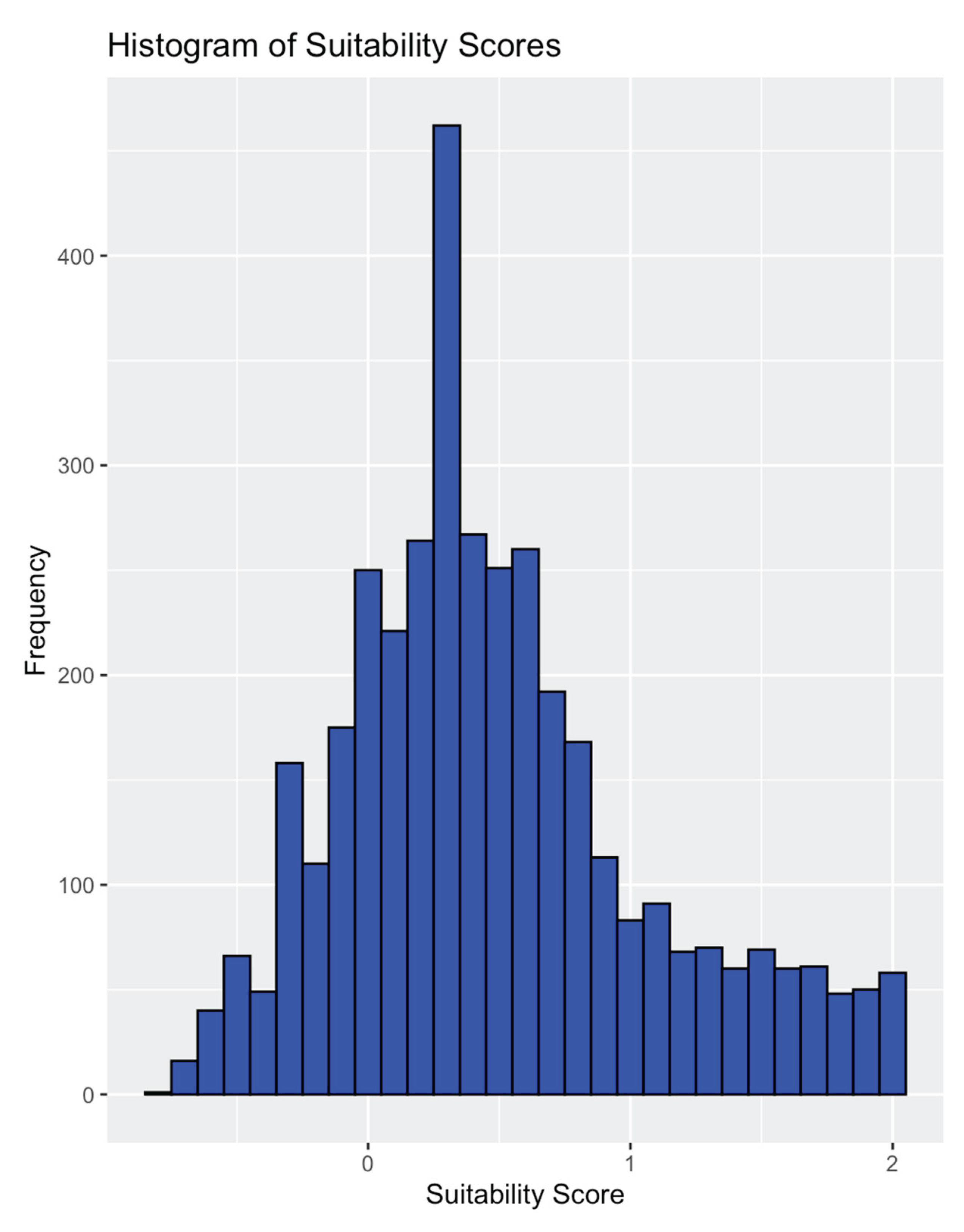
Figure 3.
Filtered Suitable Locations. Source: Estimation results, generated by the author in R.
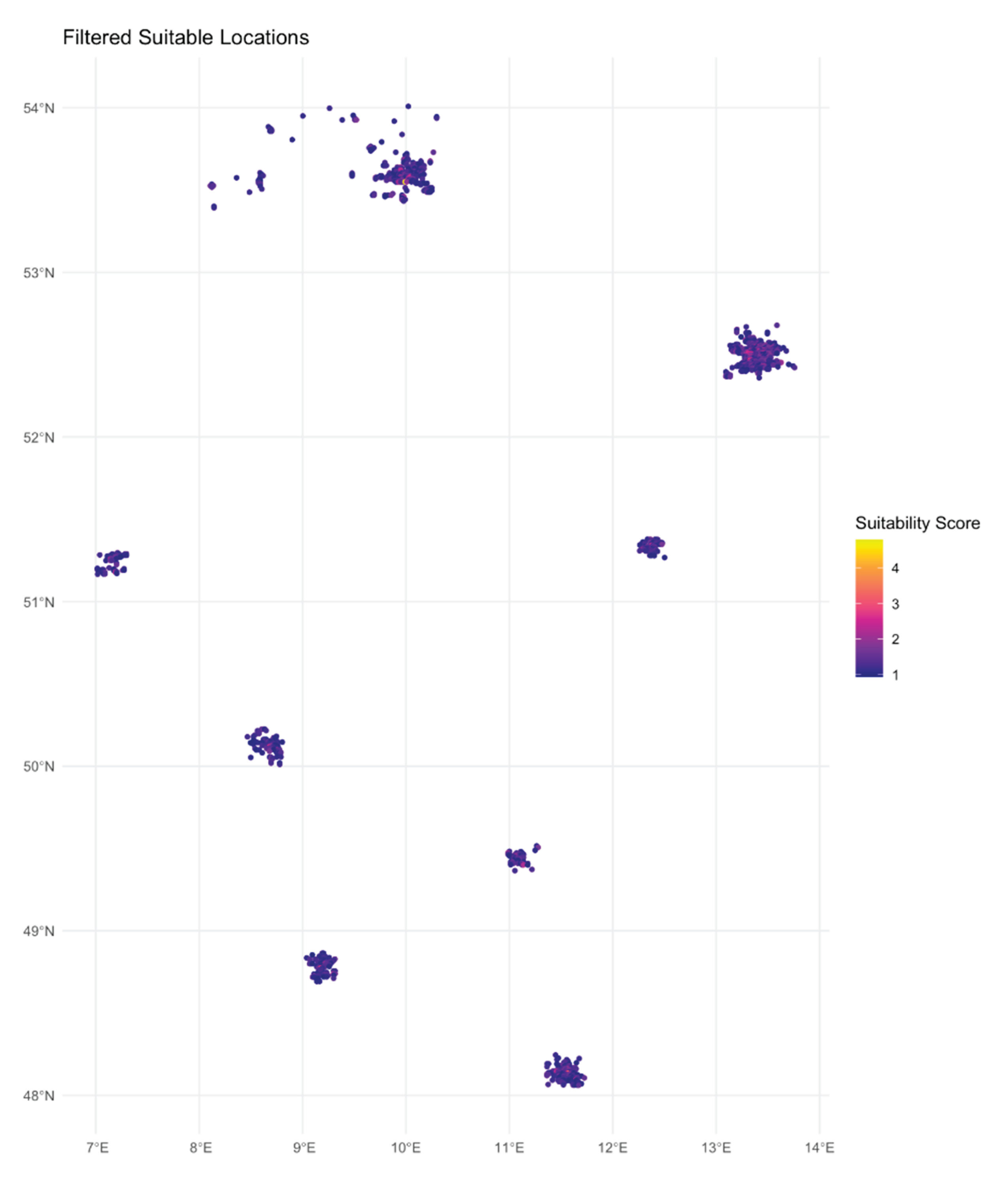
Figure 4.
Moran Scatterplot: Suitability Score vs. Spatial Lag. Source: Estimation results, generated by the author in R.
Figure 4.
Moran Scatterplot: Suitability Score vs. Spatial Lag. Source: Estimation results, generated by the author in R.
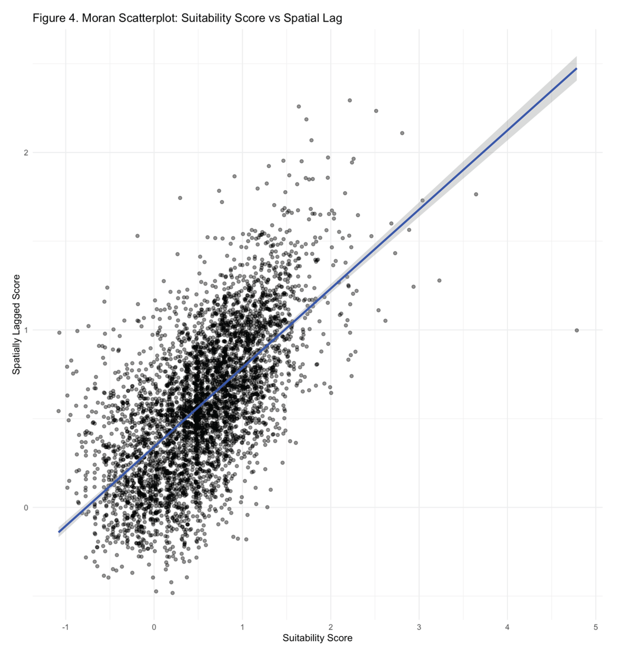
Figure 5.
Spatial clusters of suitability (LISA clusters) and corresponding suitability scores. Source: Estimation results, generated by the author in R.
Figure 5.
Spatial clusters of suitability (LISA clusters) and corresponding suitability scores. Source: Estimation results, generated by the author in R.
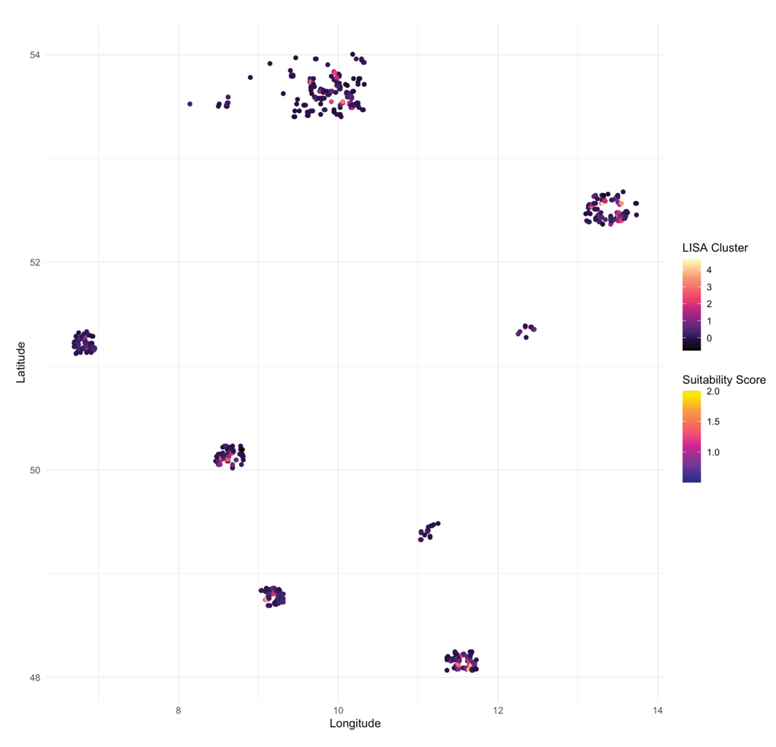
Figure 6.
Areas with high suitability score but no shops: (a) Priority cells as bubbles sized by population density and colored by suitability; (b) spatial distribution of all eligible grid cells. Source: Estimation results, generated by the author in R.
Figure 6.
Areas with high suitability score but no shops: (a) Priority cells as bubbles sized by population density and colored by suitability; (b) spatial distribution of all eligible grid cells. Source: Estimation results, generated by the author in R.
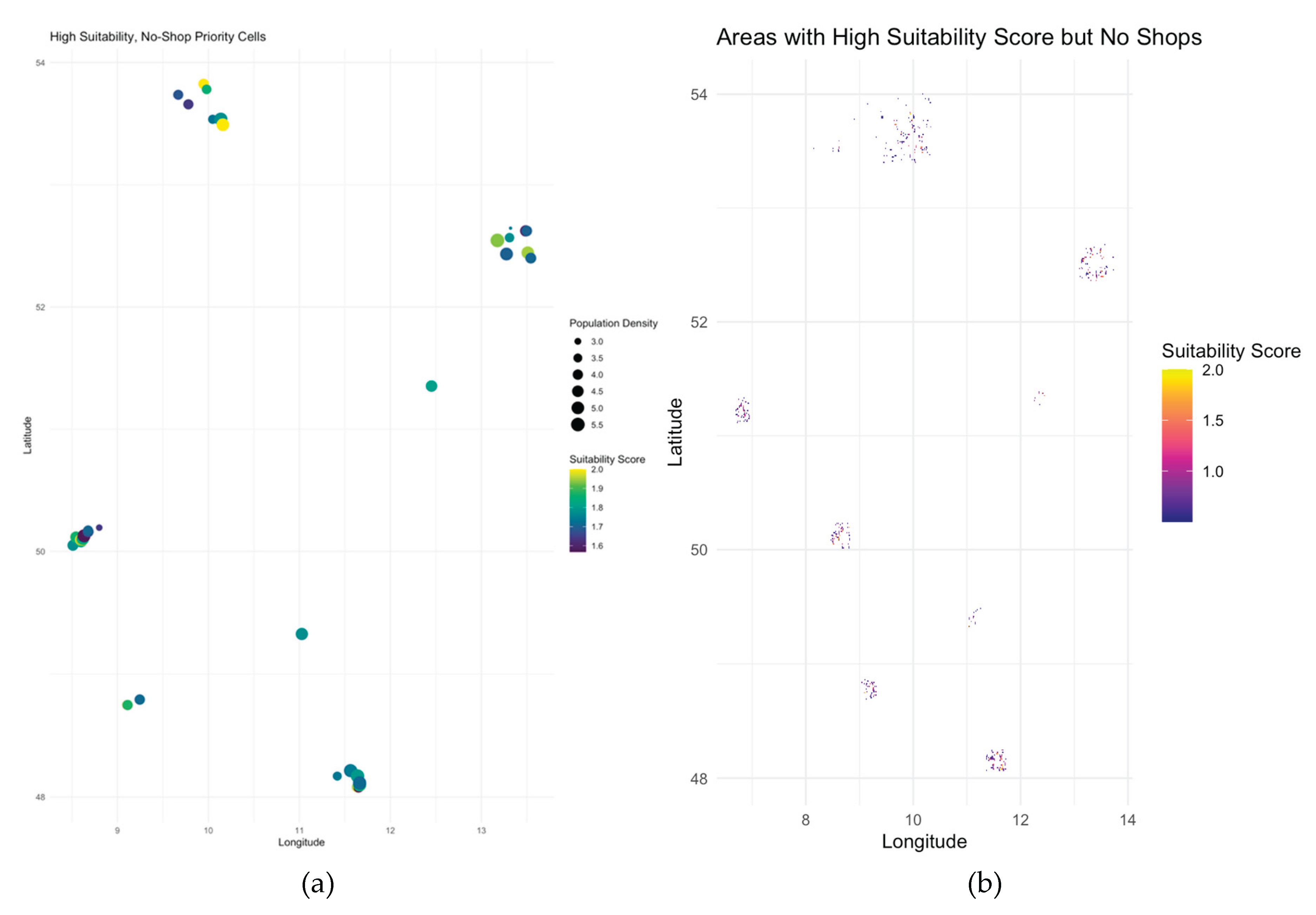
Table 1.
Dataset classification.
| Class | Population | % Female | Mean Age | Household Size |
| 1 | 3-250 | 0-40 | 0-40 | 1-2 |
| 2 | 250-500 | 40-47 | 40-42 | 2-2.5 |
| 3 | 500-2000 | 47-53 | 42-44 | 2.5-3 |
| 4 | 2000-4000 | 53-60 | 44-47 | 3-3.5 |
| 5 | 4000-8000 | >60 | >47 | >3.5 |
| 6 | >8000 |
Source: Adapted from Lovelace et al. (2019), https://r.geocompx.org/location#fig:census-stack. Table constructed and reformulated by the author.
Table 2.
Summary statistics of the socio-demographic variables.
| Statistic | Population | % Women) | Mean Age | Household Size |
| Min | 1 | 1 | 1.00 | 1.00 |
| 1st Qu. | 1 | 2 | 2.00 | 2.00 |
| Median | 1 | 3 | 3.00 | 2.00 |
| Mean | 1.49 | 2.90 | 3.06 | 2.55 |
| 3rd Qu. | 2 | 3 | 4.00 | 3.00 |
| Max | 6 | 5 | 5.00 | 5.00 |
Table 3.
Local GWR Coefficient Estimates.
| Coefficient | Min | 1st Quartile | Median | Mean | 3rd Quartile | Max |
| Population | 0.278 | 0.314 | 0.326 | 0.326 | 0.339 | 0.379 |
| Mean Age | 0.097 | 0.132 | 0.143 | 0.144 | 0.155 | 0.196 |
| POI | 0.0018 | 0.0026 | 0.0027 | 0.0027 | 0.0028 | 0.0041 |
Disclaimer/Publisher’s Note: The statements, opinions and data contained in all publications are solely those of the individual author(s) and contributor(s) and not of MDPI and/or the editor(s). MDPI and/or the editor(s) disclaim responsibility for any injury to people or property resulting from any ideas, methods, instructions or products referred to in the content. |
© 2025 by the authors. Licensee MDPI, Basel, Switzerland. This article is an open access article distributed under the terms and conditions of the Creative Commons Attribution (CC BY) license (http://creativecommons.org/licenses/by/4.0/).
Copyright: This open access article is published under a Creative Commons CC BY 4.0 license, which permit the free download, distribution, and reuse, provided that the author and preprint are cited in any reuse.


