
Submitted:
15 March 2025
Posted:
17 March 2025
You are already at the latest version
Abstract
Positional accuracy in cadastral data is fundamental for secure land tenure and efficient land administration. However, many land administration systems, experience difficulties to meet accuracy standards, particularly in areas with digitized historical maps, leading to disruptions in land transactions. This study investigates the use of unsupervised clustering algorithms in order to identify and characterize systematic spatial error patterns in cadastral maps. We compare Fuzzy c-means (FCM), Density-Based Spatial Clustering of Applications with Noise (DBSCAN), and Gaussian Mixture Models (GMM) in clustering error vectors derived from 500 homologous points. These points were obtained by comparing cadastral data with a higher-accuracy land survey within a 7 km² area in Ioannina, Greece, known for its inaccuracies in the Greek National Cadastre. The optimal number of clusters for each algorithm was determined. Results show that DBSCAN and GMM successfully captured a central area of random errors surrounded by a region exhibiting a systematic, counter-clockwise rotational error, whereas FCM did not capture this pattern. DBSCAN, with its ability to isolate noise points in the center of the study area, provided the most interpretable results. This clustering approach can be integrated into automated cadastral map improvement methods, contributing to progressive cadastral renewal efforts.
Keywords:
machine learning
; unsupervised learning
; clustering
; positional accuracy
; Greek National Cadastre
; land administration systems
; cadastral renewal
; fit-for-purpose land administration
1. Introduction
Accurate geospatial data are fundamental to the efficient operation of modern cadastral systems, supporting secure land tenure [1], effective land administration [2,3], fair taxation [4], infrastructure development [5], and reliable land transactions. Globally, modernizing Land Administration Systems (LAS) [6], and especially improving the positional accuracy of cadastral data remains an ongoing challenge. This effort is driven by the need to refine the geometric characteristics of spatial information ensuring the accurate representation of legal land objects and property boundaries [7]. Beyond initial LAS formation, there also exists the need for cadastral renewal (i.e., the process of updating, correcting, and enhancing existing cadastral data and maps). This renewal is necessary to meet accuracy standards, technological advancements, and societal needs [8,9,10] and may involve digitizing analog maps, correcting errors, updating land registry information, and integrating cadastral data with other spatial information systems [8].
Many countries have adopted cadastral renewal as a national policy to address technical and legal issues arising from outdated or inaccurate cadastral data, as illustrated by the Turkish Land Registry and Cadastre Modernization Project (TKMP) [8]. The complexity and quality of spatial data vary widely between countries, due to differences in historical development, economic resources, and organizational structures, which in turn shape the required renewal approaches [11]. Best practices in LAS management emphasize progressive improvement, where data quality is improved incrementally over time, allowing the systems to remain functional even in their early stages [12]. This method recognizes that cadastral data can exist at varying levels of encoding and accuracy, both spatially and temporally. This practice aligns with the concept of Fit-For-Purpose Land Administration (FFPLA), which proposes flexible, upgradable systems, designed to take into account local needs, resources, and land tenure types, with a focus on incremental improvement [13].
Traditional methods for enhancing positional accuracy in LAS, such as re-surveying or manual adjustments, are often costly and time-consuming. This has led the research community to explore computational correction methods that transform existing datasets using a set of homologous points (corresponding features identified in two datasets) from higher-accuracy sources [14,15,16,17]. On the other hand, automated techniques, particularly those utilizing Artificial Intelligence (AI) to minimize manual effort and improve efficiency, remain scarce, mainly in the area of vectorization [18,19].
Within AI methods, unsupervised learning algorithms uncover hidden structures in data without requiring predefined labels [20,21]. Clustering, a core unsupervised learning method [22], groups data points based on a similarity metric, such as the Euclidean distance, to uncover meaningful insights [23]. Numerous clustering methods are documented in the literature, and Oyewole and Thopil [24] provide a recent classification of these approaches. These techniques have been widely applied to spatial data analysis tasks, such as identifying patterns in geographic data, detecting hotspots, and grouping similar spatial objects [25,26,27,28].
In the context of progressive improvement of a LAS, clustering can be applied to error vectors that represent discrepancies between recorded locations on the system and more accurate survey data. If these errors have spatial structure (i.e., are not randomly distributed), clustering can identify distinct groups of points with similar error characteristics, potentially indicating systematic biases introduced during data acquirement or processing. The optimal number of clusters in unsupervised learning, which is, in general, initially unknown, is a major issue because different algorithms – or even a single algorithm with different parameters – may produce different clusters of data [29]. Hence, various methods have been developed for the determination of the optimal number of clusters (e.g., the elbow method, silhouette analysis, and information criteria) [30,31,32].
The Greek National Cadastre (GNC), like many national cadastral systems, faces ongoing challenges related to positional accuracy. Its history is marked by a series of incomplete or unsuccessful attempts to establish a comprehensive LAS [33]. Currently, it is organized under Laws 2308/1995 and 2664/1998, covering 59% of the country [34]. Despite these efforts, significant positional inaccuracies exist, particularly in areas covered by GNC first generation surveys (1995-1999). These early surveys, while aiming for 1:1000 scale accuracy in urban areas and 1:5000 in rural areas, are suffering from various issues, including systematic errors: (a) arising from the integration of administrative acts, such as land redistributions; and (b) introduced during the creation and use of photogrammetric diagrams [35].
Consequently, landowners submitted objections at an average rate of 20% of the total records (reaching up to 60% in certain areas), far exceeding the internationally accepted rate of 3–5% [34]. These discrepancies have led to legal disputes, difficulties in land transactions, and a general lack of trust in the accuracy of cadastral data. In response, the Greek State introduced Article 19A into Law 2664/1998 in 2011, enabling the en masse redefinition of land parcel positions and boundaries to support the renewal of the GNC in problematic regions.
To address these challenges, the GNC is actively exploring and implementing innovative technological solutions. In a pioneering move, it has become the first public organization in Greece to utilize Artificial Intelligence (AI) not only as a chat-bot for information, but also for making administrative decisions, aiming to accelerate the legal review process of land-related contracts. This initiative demonstrates a commitment to use advanced technologies in order to improve the effectiveness of cadastral administration [36].
This study explores the use of unsupervised clustering techniques to automatically detect and analyze systematic error patterns, focusing on a case study from Ioannina, Greece, a region from the first-generation GNC surveys, known for positional inaccuracies. The research has the following objectives: (a) to evaluate the performance of multiple clustering algorithms in the domain of spatial errors in cadastral maps; (b) to determine the optimal number of clusters for each algorithm using suitable model selection techniques; (c) to compare the performance of the algorithms using a combination of quantitative and qualitative visual assessment of the clustering results, both in the error and in the geographic space and; (d) to assess the potential of the best-performing clustering approach for generating correction models to guide automated LAS positional quality improvement.
To our knowledge, this is the first application of clustering algorithms to uncover systematic spatial errors in LASs’ data. Beyond, simply, identifying clusters, we interpret their meaning in relation to known cadastral processes and error sources, resulting in insights about data quality improvement strategies, following the philosophy of FFPLA, regarding incremental improvement, in context with the GNC needs, and its commitment using advanced technologies.
2. Data and Methods
2.1. Data and Study Area
The study area, Stavraki, is a community within the Municipality of Ioannina in the Region of Epirus, northwestern Greece (Figure 1). It spans approximately 7 square kilometers and has a mixed land use, predominantly residential areas combined with agricultural land and some commercial zones (Figure 2). Its topography consists of gently rolling hills, with an average elevation of 518 meters above sea level. The study area has been integrated into the GNC since 2005, and land records are managed by the operational cadastral office in Ioannina, responsible for maintaining property boundaries, ownership information, and related legal documentation. The region consists of 2,541 cadastral parcels, representing individual land properties.
A key characteristic of the study’s area cadastral history is the enactment of an Implementing Act under the Greek Law 1337/1983 at 2001. This Act aimed to reorganize and urbanize the land and create regularized parcels addressing the municipality’s development needs. The Act involved: (a) expropriation; (b) land contribution calculations; (c) the creation of new parcels; and (d) redistribution to the original owners. It is important to recognize that errors can be introduced at any stage of this complex Implementing Act process. The output of the Act was a map defining the final parcels with analytical coordinates. This provided a precise, mathematically defined representation of the parcel boundaries at 2001 before the development of the cadastral map for the GNC at 2005.
Despite the precise analytical definition that was provided by the Implementing Act, the study area has known problems, with professional surveyors reporting that: (a) the accuracy of the digitized cadastral map does not meet the standards of the GNC; and (b) the primary source of error is not within the Act itself, but rather in the subsequent digitization process undertaken during the creation of the GCN geodatabase at 2005 [35]. These errors, introduced during digitization, are the focus of this study.
2.2. Data Sources
The analysis uses two primary data sources:
- Land Survey Study Data: Higher-accuracy data were obtained from the digital land surveying study that was conducted by the Municipality of Ioannina in 2001 at a scale of 1:500. The survey was referenced to the Greek western zone of the Transverse Mercator (TM3 western zone) [39]. The purpose of this survey was to be the base map for the Implementing Act.
2.3. Data Preprocessing
The survey data were transformed from TM3 to HGRS87 using the second degree polynomials method, as given by the Hellenic Mapping and Cadastral Organization for this purpose [40].
To determine positional errors, homologous points were identified by comparing parcels between the 2025 data and the digital land survey of 2001. These points were selected using random sampling. Coordinate differences were calculated as:
where and Δ are the differences along the x and the y-axis, respectively, for a point . In this form, the vector represents the coordinates from the 2025 digital cadastral map and from the digital 2001 land survey, both in HGRS87. The magnitude of the error vector (i.e., the length) was also calculated for every point .
Homologous points with a length greater than 1.5 meters were excluded from the analysis, resulting to a dataset of 500 points. This threshold was used to remove potential outliers or points with gross errors, focusing the analysis on systematic error patterns rather than isolated large inaccuracies.
2.4. Clustering Algorithms
As already mentioned, clustering groups data points based on a predefined similarity measure, without prior knowledge of the group labels. In this context, the goal is to group homologous points that have similar error values , to reveal underlying spatial structure in the error distribution. If the errors were distributed randomly across the study area, clustering would likely produce arbitrary groupings without meaningful interpretation. Nonetheless, we make the hypothesis that systematic errors will be expressed as spatially district patterns. All analysis was performed using the R language [41] and the packages ‘cluster’ [42], ‘dbscan’ [43], ‘mclust’ [44], ‘factoextra’ [45], ‘ggplot2’ [46] and ‘sf’ [47].
2.4.1. Fuzzy c-Means
FCM is a clustering algorithm that extends the concept of ‘hard clustering’ (like k-means [48]) by allowing data points to belong to multiple clusters simultaneously, with varying degrees of membership [32]. This ‘fuzziness’ is particularly useful when cluster boundaries are not well-defined or when data points might have characteristics of multiple groups [49]. Initially developed by Dunn [50] and later improved by Bezdek [51], FCM aims to partition a dataset into C clusters by minimizing an objective function that considers both the distance of points to cluster centers and their membership degrees [52]. In the context of our cadastral error analysis, FCM offers a way to explore whether error patterns exhibit gradual transitions or overlapping characteristics, rather than strictly distinct, spatially separated groups. The core of FCM is the iterative minimization of the following objective function:
where: is the number of data points (homologous points, in our case); is the predefined number of clusters; is the membership degree of data point to cluster (a value between 0 and 1, where 1 represents full membership and 0 represents no membership); is the fuzzifier parameter (a real number greater than 1, controlling the level of fuzziness; typically, m = 2 [53]); is the i-th data point (the error vector; is the centroid (mean vector) of cluster ; and is the Euclidean distance between data point and cluster centroid .
The algorithm iteratively updates the membership values and the cluster centroids until convergence. The membership update equation is:
And the cluster centroid update equation is:
The algorithm stops when either a maximum number of iterations is reached or the change in the objective function between successive iterations falls below a predefined threshold, indicating convergence.
The application of FCM to our cadastral error data involves using the error vectors as input . The number of clusters, C, can be determined using the elbow method, examining the within-cluster sum of squares (WSS) [54]. The membership values and cluster centroids can then be visualized and analyzed to identify potential systematic error patterns. The algorithm was implemented using the ’fanny’ function from the cluster [42] package in R.
2.4.2. Density-Based Spatial Clustering of Applications with Noise
DBSCAN is a clustering algorithm particularly well-suited for identifying clusters of arbitrary shape and handling noise [55], making it a strong candidate to analyze cadastral error patterns. Unlike centroid-based methods, like FCM, DBSCAN does not assume that the clusters are spherical or elliptical [56]. Instead, it defines clusters based on the density of data points [57]. The algorithm operates on the basis that points within a cluster are densely packed together, while points belonging to different clusters, or noise points, are separated by regions of lower density. This density-based approach is suitable to our study because systematic errors in cadastral data may have spatial patterns that are linear or curved.
The DBSCAN algorithm is based on two key parameters [55,57]: (a) that defines the radius of a neighborhood around each data point; and (b) that specifies the minimum number of data points required within the radius for a point to be considered a ‘core point’. These parameters are used to define the -neighborhood of a point :
where is the dataset of points and is the Euclidean distance between points and . A core point is one point if its -neighborhood contains at least points:
A point is directly density-reachable from a point if is within the -neighborhood of a point , and is core point:
A point is density-reachable from a point if there exists a chain of points where and , and each is directly density-reachable from . Two points and are density-connected if there exists a point such that both are density-reachable from . A cluster is a set of density-connected points that is maximal with respect to density-reachability. Noise points are points that are not density-reachable from any other point. The algorithm proceeds iteratively, by examining each point and applying these definitions.
In our cadastral error analysis, the input data points to DBSCAN are the error vectors (. The parameter describes a distance in the error space, and represents the minimum number of points with similar error magnitudes and directions required to form a cluster. A suitable parameter can be selected using the k-nearest neighbor (kNN) distances for the dataset represented as a matrix of points [57]. The kNN distance is defined as the distance from a point to its k nearest neighbor. The algorithm was implemented using the ‘kNNdistplot’ and ’dbscan’ functions from the `dbscan` R package [43].
2.4.3. Gaussian Mixture Models
GMM is a probabilistic model that assumes that data points are generated from a mixture of several Gaussian distributions [58]. It’s a form of soft clustering, like FCM, assigning probabilities that a point belongs to each cluster [59].
The core concept of GMMs is to represent the overall probability density function (PDF) of the data as a weighted sum of individual Gaussian component densities. The PDF for a GMM with K components has parameters and is given by [59,60,61]:
where: is the number of Gaussian components (clusters), is the data point, is the mixing coefficient for the k-th component, representing the prior probability of a data point belonging to that component ( and ), is the multivariate Gaussian probability density function for the k-th component, defined by:
where: is the vector of means, is the covariance matrix, is the determinant and denotes the transpose. The GMM algorithm typically uses the Expectation-Maximization (EM) algorithm to estimate the parameters that maximize the likelihood of the observed data [62]. The EM algorithm iteratively performs two steps:
- Expectation (E-step): Calculates the posterior probability of each component for each data point, given the current parameter estimates. This represents the probability that a data point belongs to a particular Gaussian component;
- Maximization (M-step): Updates the parameters
to maximize the likelihood of the data, given the posterior probabilities calculated in the E-step.
These steps are repeated until convergence, by monitoring the change in the log-likelihood of the data [59].
In our analysis, the GMM is, also, applied to the error vectors . The number of components, G, can be determined using the Bayesian Information Criterion (BIC) for various predefined covariance models [59]. The EM algorithm then estimates the parameters of each Gaussian component. The ability of GMM to model elliptical clusters makes them suitable to capture additionally linear error patterns. The GMM was implemented using the `Mclust` function from the `mclust` package in R [44].
2.3.5. Selection of the Algorithms
The algorithms FCM, DBSCAN and GMM were selected due to the diverse clustering methodologies that they represent: (a) DBSCAN for its ability to identify clusters of arbitrary shape; (b) GMM for its probabilistic assumptions and its flexibility to model elliptical clusters, and (c) FCM for its assumption that points may belong to multiple clusters [52].
Another factor in algorithm selection was robustness to noise, as cadastral datasets often contain outliers. DBSCAN distinguishes noise from meaningful clusters by design [57], while GMM can address some degree of noise through its probabilistic framework [59]. However, FCM tends to be more sensitive to outliers [52], a fact that demands thorough preprocessing of the data.
Regarding the need to select in advance the number of clusters, while DBSCAN theoretically offers the advantage of automatically selection, this is indirectly linked to the values of its parameters, and especially ε that defines the neighborhood radius which influences clustering results [32]. Both FCM and GMM demand a priori the number of clusters as an input parameter of the algorithms, which can be determined using the aforementioned model selection methods.
Finally, all three algorithms are available as, well documented, open-source software in the R language, ensuring accessibility and ease of implementation. Summarizing, the selection of these methods allows a comprehensive evaluation of clustering algorithm’s effectiveness in cadastral error pattern recognition.
2.3.6. Evaluation and Clustering Validity
The evaluation and comparison of the clustering results from FCM, DBSCAN, and GMM algorithms comprise both arithmetic indices and visual assessments. The quantitative metric used in the study is the silhouette score [63], which measures the unity and separation of clusters. This score ranges from -1 to +1, with higher values indicating well-defined clusters. Nevertheless, given its known limitations [64], particularly in assessing non-spherical clusters, we emphasize on visual inspection of the results to insure that they are meaningful.
Qualitative assessment is necessary in evaluating clustering effectiveness through the visual examination of: (a) error vector plots; and (b) spatial distribution plots. Error vector plots, where points are colored according to the cluster that they belong, offer insights into the separation and shape of clusters within the error space. More essentially, spatial distribution plots reveal the geographic classification of homologous points in clusters, helping to determine whether these clusters create meaningful results in the actual space.
3. Results
3.1. Exploratory Analysis
To characterize the discrepancies between the 2025 cadastral map and the 2001 land survey, we calculated the error vectors (ΔE,ΔΝ) and their Euclidean distances (L) of the 500 homologous points. Table 1 presents descriptive statistics about the distribution of these error values. Prior the application of data filtering, the root mean squared error (RMSE) on the plane of the study area was m, a value that surpasses the current GNC’s geometric accuracy criterion of [65].
The key observations about these values are:
- Mean Error: The mean is close to zero (0.03 m), while the mean Δ is considerably larger and negative (-0.50 m). This indicates a systematic shift in the Northing direction between the 2025 and the 2001 data;
- Symmetry: The near-zero skewness values for both and Δ suggest that the error distributions are approximately symmetric, although Δ has a slight positive skew;
- Tails: The negative kurtosis for ΔE indicates a platykurtic distribution that has lighter tails and a flatter peak compared to a normal distribution, whereas the positive value for ΔN is a leptokurtic distribution with heavier tails and sharper peak;
- Variability: The CV for (10.67) is substantially larger than that for ΔNorth (0.66), indicating greater relative variability in the Easting errors compared to the Northing errors;
- Skewness: Near-zero values suggest approximately symmetric distributions;
- Kurtosis: Low values indicate light tails, consistent with normal-like distributions;
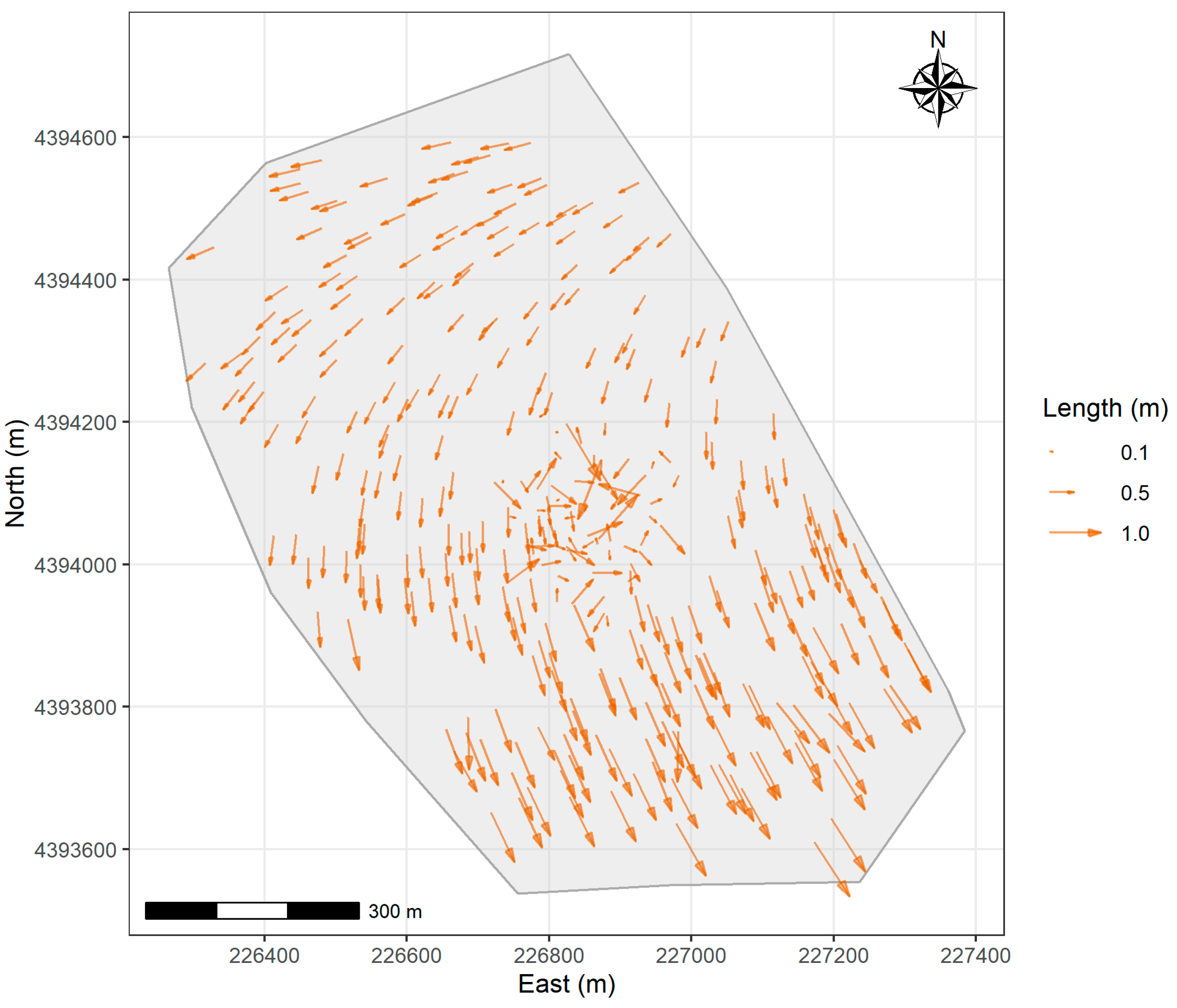
Figure 2 depicts the spatial distribution of (ΔE,ΔΝ). The length of each vector represents the magnitude of the error and its direction indicates the orientation of the discrepancy. This vector plot reveals that the errors are not randomly distributed across the study area, but instead have a clear spatial structure. While a small area in the central portion of the study area shows random error orientations and magnitudes, the dominant pattern across the rest of the region is a ring-like, counter-clockwise rotation. This pattern suggests a systematic transformation error, introduced during the integration of the Implementation Act map to the 2005 cadastral framework.
Figure 3.
Vector plot of positional errors in the study area.
3.2. Optimal Number of Clusters
The optimal number of clusters for each algorithm was determined as follows:
- FCM: The elbow method was used, examining the WSS value as a function of the number of clusters (Figure 4). A distinct ‘elbow’ is observed between 2 and 4 clusters, and the mean value of 3 was selected.
- DBSCAN: The 5-nearest neighbor distance plot (Figure 5) was examined. A visible ‘knee’ is observed around a distance of 0.10. Therefore, an ε value of 0.10 was selected. Additionally, a value of 10 points was chosen, as it appeared suitable for capturing meaningful cluster structures within the dataset.
3.2. Clustering Results - Visualizations
Figure 7, Figure 8 and Figure 9 depict the clustering results for each algorithm. The left panels show the error vector plot ΔΕ versus ΔΝ (i.e., in the error space), and the right ones depict the spatial distribution plot (i.e., in the actual space).
Regarding the error vector plots for each clustering algorithm:
- FCM (Figure 7a): Three relatively well-separated clusters are formed. However, they don’t capture the obvious linear pattern in the error space.
- DBSCAN (Figure 8a): The clear linear cluster (blue points) is identified as well as a large number of noise points (red points). The linear cluster matches the suspected systematic error.
- Regarding the spatial distribution plots for each clustering algorithm:
- DBSCAN (Figure 8b): The blue points (the linear cluster) form a distinct, spatially contiguous region covering the majority of the study area, matching the area where we observed the ring-like, counter-clockwise rotational error pattern in Figure 3. The red noise points are concentrated in the central area.
- GMM (Figure 9b): The spatial distribution is very similar to DBSCAN, with the blue points forming a contiguous region corresponding to the rotational error. Most of the ‘noise’ points from DBSCAN now form the red cluster, making the distinction of signal to noise less clear.
3.3. Quantitative Evaluation—Silhouette Scores
The mean silhouette scores for each algorithm are presented in Table 2, with FCM achieving the highest score, followed by DBSCAN and GMM. However, interpreting these scores in the context of the cadastral error patterns of the study area requires caution. The silhouette score inherently favors compact, spherical clusters, making it less suitable for evaluating clustering methods that capture more complex, non-spherical structures. DBSCAN and GMM, which captured the non-spherical linear pattern, have lower silhouette scores but provide meaningful results.
3.3. Cluster Characteristics
Table 3 summarizes the key statistics of the clusters identified by the three algorithms, including the number of points, mean displacement in the east and north directions, standard deviations, and mean error vector length. These statistics provide insights into the spatial patterns and magnitudes of cadastral errors captured by each algorithm.
DBSCAN effectively captures the systematic error pattern in Cluster 1, with a mean ΔΝ of -0.57 m, confirming a consistent southward shift. Meanwhile, noise points display a smaller mean error but high standard deviation, indicating greater variability.
GMM achieves similar results but forces all points into clusters, making the distinction between the systematic error and noise less clear. FCM, while producing well-separated clusters in the error space, fails to capture the spatial structure of the errors, demonstrating its unsuitability for this particular problem.
The systematic error identified by both DBSCAN and GMM is characterized by a counter-clockwise rotation and a significant southward shift in a ring-shaped area. This strongly confirms the issue during the digitization of the Implementation Act, where a transformation (likely involving a rotation and translation) was incorrectly applied to a large portion of the study area. The points identified as noise by DBSCAN and as the cluster number one by GMM represent the central area that has more complex, non-systematic errors.
4. Discussion
This study highlights that unsupervised machine learning algorithms can efficiently identify and characterize systematic spatial errors in cadastral data. The detection of a district ring-shaped region affected by a systematic error in the study area reveals an issue introduced during the digitization process of the Implementation Act to the GNC. This finding depicts the challenges that may arise in order to improve the positional accuracy in LASs, particularly when data are coming from various sources and historical maps [66,67,68]. It also highlights the need of cadastral renewal, to address errors and inconsistencies, as reported in the literature.
The comparison of the algorithms emphasizes the importance of choosing one appropriate to the specific domain’s data structure, in our case real-world cadastral data. While FCM produced well-separated clusters in the actual space, its assumption of spherical clusters limited its ability to capture the obvious spatial structure in the error space. DBSCAN, with its ability to identify clusters of arbitrary shape and its robustness to noise proved to be more effective algorithm. GMM performed equally well in identifying the linear pattern, but lacks the property of explicit noise handling, although it recognized as a different cluster the region at the center of the study area that has random errors.
While popular, the silhouette score, a quantitative measure of cluster quality, requires cautious interpretation in the specific dataset. The higher score for FCM does not agree with its performance. This underscores the importance of not relying only on quantitative metrics, but also use qualitative methods to evaluate whether clustering algorithms produce meaningful results.
The findings of this study have a direct application to the GNC. The identified region with the systematic error provides a clear target for corrections. Instead of conducting a re-survey of the entire area, resources can be directed to this region, using a simple transformation of the parcels, such as the Helmert transformation [69] to address the issue. This approach has the potential to reduce the cost and time required for cadastral map improvement in Greece.
Additionally, our results support the principles of FFPLA [13]. Clustering can be used as a ‘minimum viable’ method to identify and prioritize areas for improvement, supporting the FFPLA concept of upgradability. The identified clusters represent areas where the cadastral data are not currently ‘fit-for-purpose’ in terms of positional accuracy, and the clustering results provide a roadmap for targeted and economical corrections.
Finally, the identified clusters could also serve as input data for other supervised machine learning algorithms that can transform the cadastral map, in order to improve its positional accuracy. Despite the growing adoption of AI in geospatial analysis, AI-driven methods have not yet been widely applied to geometric corrections in LAS and this study highlights their potential.
5. Conclusions
This study demonstrates that unsupervised algorithms can effectively identify and characterize systematic spatial errors in digital cadastral maps. This automated identification of problematic regions has a significant practical value for the Greek National Cadastre, enabling targeted and cost-effective correction efforts, and directly contributes to the broader goals of cadastral renewal and progressive improvement.
This research has limitations because the analysis focus on a single study area. Therefore, findings may not generalize directly to other regions or countries. In addition, while clustering identifies the presence and location of systematic errors, it does not, by itself, provide the solution to correct them. Therefore, further work is needed towards the development of automated improvement methods.
Future research should validate this methodology on a larger set of areas, incorporate additional data sources to reveal error causes, and explore other clustering and machine learning approaches. Integrating expert knowledge through semi-supervised or active learning could improve results. Future work should focus on developing automated correction methods based on these findings, leading to a streamlined workflow for cadastral map improvement, with a goal for more reliable, fit-for-purpose, land administration systems.
Author Contributions
Conceptualization, methodology, K.V.; data curation, V.M.; writing—original draft preparation, K.V.; writing—review and editing, V.M. All authors have read and agreed to the published version of the manuscript.
Funding
This research received no external funding.
Data Availability Statement
The shape files of the parcels from the study area are available at the website of GNC: https://data.ktimatologio.gr/. The Implementation Act is available at the Unified Digital Map portal of the Technical Chamber of Greece at https://psifiakosxartistee.gr/.
Acknowledgments
This research was made possible by the generous support of the Cadastral Office of Ioannina, which provided access to the necessary cadastral and survey data for the study area, and shared valuable insights about the existing positional accuracy issues. During the preparation of this work the authors used Gemini 2.0 Pro in order to improve the text’s spelling and grammar. After using this tool, the authors reviewed and edited the content as needed and take full responsibility for the content of the publication.
Conflicts of Interest
The authors declare no conflicts of interest.
Abbreviations
The following abbreviations are used in this manuscript:
| AI | Artificial Intelligence |
| BIC | Bayesian Information Criterion |
| CV | Coefficient of Variation |
| DBSCAN | Density-Based Spatial Clustering of Applications with Noise |
| EM | Expectation Maximization |
| FCM | Fuzzy c-means |
| FFPLA | Fit-For-Purpose Land Administration |
| FIG | International Federation of Surveyors |
| GCN | Greek National Cadastre |
| GMM | Gaussian Mixture Model |
| HGRS87 | Hellenic Geodetic Reference System 1987 |
| kNN | k-Nearest Neighbor |
| LAS | Land Administration Systems |
| Probability Density Function | |
| RMSE | Root Mean Squared Error |
| SD | Standard Deviation |
| TKMP | Turkish Land Registry and Cadastre Modernization Project |
| TM | Transverse Mercator |
| WSS | Within-cluster Sum of Squares |
References
- Movahhed Moghaddam, S.; Azadi, H.; Sklenička, P.; Janečková, K. Impacts of Land Tenure Security on the Conversion of Agricultural Land to Urban Use. Land Degradation & Development 2025. [CrossRef]
- Bydłosz, J. The Application of the Land Administration Domain Model in Building a Country Profile for the Polish Cadastre. Land Use Policy 2015, 49, 598–605. [Google Scholar] [CrossRef]
- Uşak, B.; Çağdaş, V.; Kara, A. Current Cadastral Trends—A Literature Review of the Last Decade. Land 2024, 13, 2100. [Google Scholar] [CrossRef]
- Aguzarova, L.A.; Aguzarova, F.S. On the Issue of Cadastral Value and Its Impact on Property Taxation in the Russian Federation. In Business 4.0 as a Subject of the Digital Economy; Popkova, E.G., Ed.; Advances in Science, Technology & Innovation; Springer International Publishing: Cham, 2022; ISBN 978-3-030-90323-7. [Google Scholar]
- El Ayachi, M.; Semlali, E.H. Digital Cadastral Map, a Multipurpose Tool for Sustainable Development. In Proceedings of the Proceeding of the International conference on spatial information for sustainable development, Nairobi; 2001; pp. 2–5. [Google Scholar]
- Jahani Chehrehbargh, F.; Rajabifard, A.; Atazadeh, B.; Steudler, D. Current Challenges and Strategic Directions for Land Administration System Modernisation in Indonesia. Journal of Spatial Science 2024, 69, 1097–1129. [Google Scholar] [CrossRef]
- Hashim, N.M.; Omar, A.H.; Ramli, S.N.M.; Omar, K.M.; Din, N. Cadastral Database Positional Accuracy Improvement. Int. Arch. Photogramm. Remote Sens. Spatial Inf. Sci. 2017, XLII-4/W5, 91–96. [CrossRef]
- Ercan, O. Evolution of the Cadastre Renewal Understanding in Türkiye: A Fit-for-Purpose Renewal Model Proposal. Land Use Policy 2023, 131, 106755. [Google Scholar] [CrossRef]
- Kysel’, P.; Hudecová, L. Testing of a New Way of Cadastral Maps Renewal in Slovakia. 2022.
- Lauhkonen, H. Cadastral Renewal in Finland-The Challenges of Implementing LIS. GIM international 2007, 21, 42. [Google Scholar]
- Roić, M.; Križanović, J.; Pivac, D. An Approach to Resolve Inconsistencies of Data in the Cadastre. Land 2021, 10, 70. [Google Scholar] [CrossRef]
- Thompson, R.J. A Model for the Creation and Progressive Improvement of a Digital Cadastral Data Base. Land use policy 2015, 49, 565–576. [Google Scholar] [CrossRef]
- Bennett, R.M.; Unger, E.-M.; Lemmen, C.; Dijkstra, P. Land Administration Maintenance: A Review of the Persistent Problem and Emerging Fit-for-Purpose Solutions. Land 2021, 10, 509. [Google Scholar] [CrossRef]
- Morgenstern, D.; Prell, K.M.; Riemer, H.G. Digitisation and Geometrical Improvement of Inhomogeneous Cadastral Maps. Survey Review 1989, 30, 149–159. [Google Scholar] [CrossRef]
- Tamim, N.S. A Methodology to Create a Digital Cadastral Overlay through Upgrading Digitized Cadastral Data, The Ohio State University: Ohio, USA, 1992.
- Tuno, N.; Mulahusić, A.; Kogoj, D. Improving the Positional Accuracy of Digital Cadastral Maps through Optimal Geometric Transformation. Journal of surveying engineering 2017, 143, 05017002. [Google Scholar] [CrossRef]
- Čeh, M.; Gielsdorf, F.; Trobec, B.; Krivic, M.; Lisec, A. Improving the Positional Accuracy of Traditional Cadastral Index Maps with Membrane Adjustment in Slovenia. ISPRS international journal of geo-information 2019, 8, 338. [Google Scholar] [CrossRef]
- Franken, J.; Florijn, W.; Hoekstra, M.; Hagemans, E. Rebuilding the Cadastral Map of The Netherlands, the Artificial Intelligence Solution. In Proceedings of the FIG working week; Amsterdam, the Netherlands; 2020. [Google Scholar]
- Petitpierre, R.; Guhennec, P. Effective Annotation for the Automatic Vectorization of Cadastral Maps. Digital Scholarship in the Humanities 2023, 38, 1227–1237. [Google Scholar] [CrossRef]
- Hastie, T.; Friedman, J.; Tibshirani, R. The Elements of Statistical Learning; Springer Series in Statistics; Second Edition. Springer New York: New York, USA, 2001; ISBN 978-1-4899-0519-2. [Google Scholar]
- Tyagi, A.K.; Chahal, P. Artificial Intelligence and Machine Learning Algorithms. In Challenges and applications for implementing machine learning in computer vision; IGI Global Scientific Publishing, 2020; pp. 188–219.
- Hartigan, J.A. Clustering Algorithms; John Wiley & Sons Inc: NY, USA, 1975; ISBN 978-0-471-35645-5. [Google Scholar]
- Jain, A.K.; Duin, R.P.W.; Mao, J. Statistical Pattern Recognition: A Review. IEEE Transactions on Pattern Analysis and Machine Intelligence 2000, 22, 4–37. [Google Scholar] [CrossRef]
- Oyewole, G.J.; Thopil, G.A. Data Clustering: Application and Trends. Artif Intell Rev 2023, 56, 6439–6475. [Google Scholar] [CrossRef]
- Han, J.; Pei, J.; Tong, H. Data Mining: Concepts and Techniques; Morgan kaufmann, 2022.
- Grubesic, T.H.; Wei, R.; Murray, A.T. Spatial Clustering Overview and Comparison: Accuracy, Sensitivity, and Computational Expense. Annals of the Association of American Geographers 2014, 104, 1134–1156. [Google Scholar] [CrossRef]
- Wang, H.; Song, C.; Wang, J.; Gao, P. A Raster-Based Spatial Clustering Method with Robustness to Spatial Outliers. Scientific Reports 2024, 14, 4103. [Google Scholar]
- Xie, Y.; Shekhar, S.; Li, Y. Statistically-Robust Clustering Techniques for Mapping Spatial Hotspots: A Survey. ACM Comput. Surv. 2023, 55, 1–38. [Google Scholar] [CrossRef]
- Vantas, K.; Sidiropoulos, E.; Loukas, A. Robustness Spatiotemporal Clustering and Trend Detection of Rainfall Erosivity Density in Greece. Water 2019, 11, 1050. [Google Scholar] [CrossRef]
- Milligan, G.W.; Cooper, M.C. An Examination of Procedures for Determining the Number of Clusters in a Data Set. Psychometrika 1985, 50, 159–179. [Google Scholar] [CrossRef]
- Charrad, M.; Ghazzali, N.; Boiteau, V.; Niknafs, A. NbClust: An R Package for Determining the Relevant Number of Clusters in a Data Set. Journal of statistical software 2014, 61, 1–36. [Google Scholar] [CrossRef]
- Vantas, K.; Sidiropoulos, E. Intra-Storm Pattern Recognition through Fuzzy Clustering. Hydrology 2021, 8, 57. [Google Scholar] [CrossRef]
- Potsiou, C.; Volakakis, M.; Doublidis, P. Hellenic Cadastre: State of the Art Experience, Proposals and Future Strategies. Computers, Environment and Urban Systems 2001, 25, 445–476. [Google Scholar] [CrossRef]
- Arvanitis, A. Cadastre 2020; Editions Ziti: Thessaloniki, Greece, 2014; ISBN 978-960-456-423-1. [Google Scholar]
- Vantas, K. Improving the positional accuracy of cadastral maps via Machine Learning methods, Aristotle University of Thessaloniki: Thessaloniki, Greece, 2022.
- Cadastre: The First Public Agency to Integrate Artificial Intelligence (in Greek) Available online:. Available online: https://www.ktimatologio.gr/grafeio-tipou/deltia-tipou/1493 (accessed on 10 March 2025).
- Greek National Cadastre - Open Data Portal Available online:. Available online: https://data.ktimatologio.gr/ (accessed on 11 March 2025).
- Veis, G. Reference systems and the realization of the Hellenic Geodetic Reference System 1987; Technika Chronika; Technical Chamber of Greece: Athens, Greece, 1995. [Google Scholar]
- Fotiou, A.; Livieratos, E. Geometric geodesy and networks; Editions Ziti: Thessaloniki, Greece, 2000; ISBN 960-431-612-5. [Google Scholar]
- Hellenic Mapping and Cadastral Organization Tables of coefficients for coordinates transformation of the Hellenic area; HEMCO: Athens, Greece, 1995.
- R Core Team, R. R: A Language and Environment for Statistical Computing. Foundation for statistical computing Vienna, Austria 2025.
- Maechler, M.; original), P.R. (Fortran; original), A.S. (S; original), M.H. (S; Hornik [trl, K.; maintenance(1999-2000)), ctb] (port to R.; Studer, M.; Roudier, P.; Gonzalez, J.; Kozlowski, K.; et al. Cluster: “Finding Groups in Data”: Cluster Analysis Extended Rousseeuw et Al. 2024.
- Hahsler, M.; Piekenbrock, M.; Arya, S.; Mount, D.; Malzer, C. Dbscan: Density-Based Spatial Clustering of Applications with Noise (DBSCAN) and Related Algorithms 2025.
- Fraley, C.; Raftery, A.E.; Scrucca, L.; Murphy, T.B.; Fop, M. Mclust: Gaussian Mixture Modelling for Model-Based Clustering, Classification, and Density Estimation 2024.
- Kassambara, A.; Mundt, F. Factoextra: Extract and Visualize the Results of Multivariate Data Analyses 2020.
- Wickham, H.; Chang, W.; Henry, L.; Pedersen, T.L.; Takahashi, K.; Wilke, C.; Woo, K.; Yutani, H.; Dunnington, D.; Brand, T. van den; et al. Ggplot2: Create Elegant Data Visualisations Using the Grammar of Graphics 2024.
- Pebesma, E.; Bivand, R.; Racine, E.; Sumner, M.; Cook, I.; Keitt, T.; Lovelace, R.; Wickham, H.; Ooms, J.; Müller, K.; et al. Sf: Simple Features for R 2024.
- Bishop, C.M.; Nasrabadi, N.M. Pattern Recognition and Machine Learning; Springer, 2006; Vol. 4.
- Sarle, W.S. Finding Groups in Data: An Introduction to Cluster Analysis 1991.
- Dunn, J.C. A Fuzzy Relative of the ISODATA Process and Its Use in Detecting Compact Well-Separated Clusters. Journal of Cybernetics 1973, 3, 32–57. [Google Scholar] [CrossRef]
- Bezdek, J.C. Pattern Recognition with Fuzzy Objective Function Algorithms; Springer Science & Business Media, 2013.
- Nayak, J.; Naik, B.; Behera, H.S. Fuzzy C-Means (FCM) Clustering Algorithm: A Decade Review from 2000 to 2014. In Proceedings of the Computational Intelligence in Data Mining - Volume 2; Jain, L.C., Behera, H.S., Mandal, J.K., Mohapatra, D.P., Eds.; Springer India: New Delhi, 2015; pp. 133–149. [Google Scholar]
- Huang, M.; Xia, Z.; Wang, H.; Zeng, Q.; Wang, Q. The Range of the Value for the Fuzzifier of the Fuzzy C-Means Algorithm. Pattern Recognition Letters 2012, 33, 2280–2284. [Google Scholar]
- Syakur, M.A.; Khotimah, B.K.; Rochman, E.M.S.; Satoto, B.D. Integration K-Means Clustering Method and Elbow Method for Identification of the Best Customer Profile Cluster. In Proceedings of the IOP conference series: materials science and engineering; IOP Publishing, 2018; Vol. 336; p. 012017. [Google Scholar]
- Ester, M.; Kriegel, H.-P.; Sander, J.; Xu, X. Density-Based Spatial Clustering of Applications with Noise. In Proceedings of the Int. Conf. knowledge discovery and data mining; 1996; Vol. 240. [Google Scholar]
- Kriegel, H.; Kröger, P.; Sander, J.; Zimek, A. Density-based Clustering. WIREs Data Min & Knowl 2011, 1, 231–240. [Google Scholar] [CrossRef]
- Hahsler, M.; Piekenbrock, M.; Doran, D. Dbscan: Fast Density-Based Clustering with R. Journal of Statistical Software 2019, 91, 1–30. [Google Scholar] [CrossRef]
- Reynolds, D.A. Gaussian Mixture Models. Encyclopedia of biometrics 2009, 741, 3. [Google Scholar]
- Scrucca, L.; Fraley, C.; Murphy, T.B.; Raftery, A.E. Model-Based Clustering, Classification, and Density Estimation Using Mclust in R; Chapman and Hall/CRC, 2023; ISBN 978-1-032-23495-3.
- Scrucca, L.; Fop, M.; Murphy, T.B.; Raftery, A.E. Mclust 5: Clustering, Classification and Density Estimation Using Gaussian Finite Mixture Models. The R journal 2016, 8, 289. [Google Scholar]
- Fraley, C.; Raftery, A.E. Model-Based Clustering, Discriminant Analysis, and Density Estimation. Journal of the American Statistical Association 2002, 97, 611–631. [Google Scholar] [CrossRef]
- Yang, M.-S.; Lai, C.-Y.; Lin, C.-Y. A Robust EM Clustering Algorithm for Gaussian Mixture Models. Pattern Recognition 2012, 45, 3950–3961. [Google Scholar] [CrossRef]
- Shahapure, K.R.; Nicholas, C. Cluster Quality Analysis Using Silhouette Score. In Proceedings of the 2020 IEEE 7th international conference on data science and advanced analytics (DSAA); IEEE; 2020; pp. 747–748. [Google Scholar]
- Arbelaitz, O.; Gurrutxaga, I.; Muguerza, J.; Pérez, J.M.; Perona, I. An Extensive Comparative Study of Cluster Validity Indices. Pattern recognition 2013, 46, 243–256. [Google Scholar] [CrossRef]
- Hellenic Republic Approval of technical specifications and the regulation of estimated fees for cadastral survey studies for the creation of the National Cadastre in the remaining areas of the country; Ministry of Environment and Energy: Athens, Greece, 2016; p. 228.
- Sisman, Y. Coordinate Transformation of Cadastral Maps Using Different Adjustment Methods. Journal of the Chinese Institute of Engineers 2014, 37, 869–882. [Google Scholar] [CrossRef]
- Tong, X.; Liang, D.; Xu, G.; Zhang, S. Positional Accuracy Improvement: A Comparative Study in Shanghai, China. International Journal of Geographical Information Science 2011, 25, 1147–1171. [Google Scholar] [CrossRef]
- Manzano-Agugliaro, F.; Montoya, F.G.; San-Antonio-Gómez, C.; López-Márquez, S.; Aguilera, M.J.; Gil, C. The Assessment of Evolutionary Algorithms for Analyzing the Positional Accuracy and Uncertainty of Maps. Expert Systems with Applications 2014, 41, 6346–6360. [Google Scholar] [CrossRef]
- Watson, G.A. Computing Helmert Transformations. Journal of computational and applied mathematics 2006, 197, 387–394. [Google Scholar] [CrossRef]
Figure 1.
study area location in Greece (dark blue box). Reference System: HGRS87 (Hellenic Geodetic Reference System 1987).
Figure 1.
study area location in Greece (dark blue box). Reference System: HGRS87 (Hellenic Geodetic Reference System 1987).
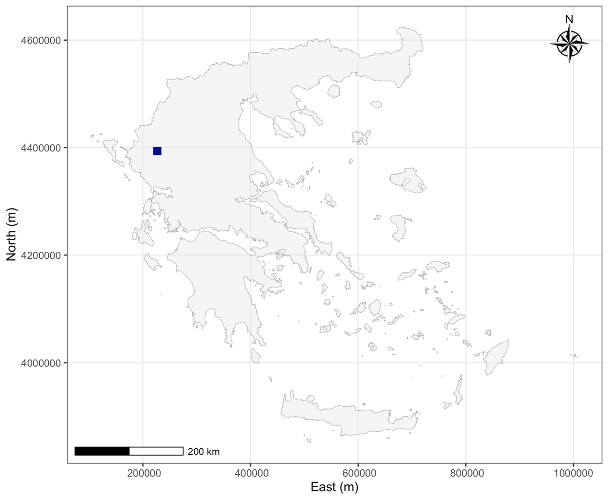
Figure 2.
Orthophoto map of the study area with yellow (2015). At the east of the study area is the city of Ioannina. Source: National Cadastre of Greece.
Figure 2.
Orthophoto map of the study area with yellow (2015). At the east of the study area is the city of Ioannina. Source: National Cadastre of Greece.
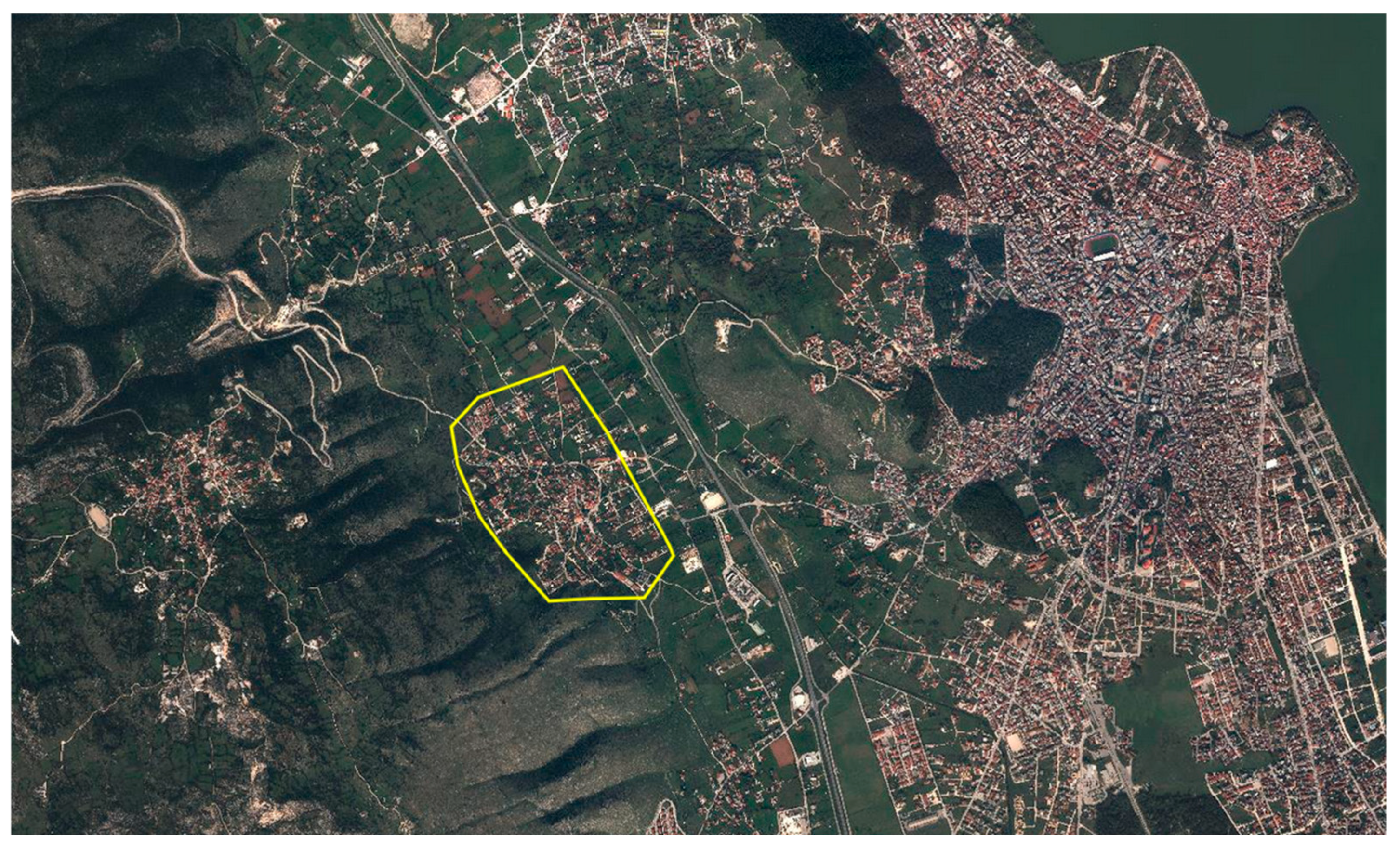
Figure 4.
Elbow plot for the FCM algorithm.
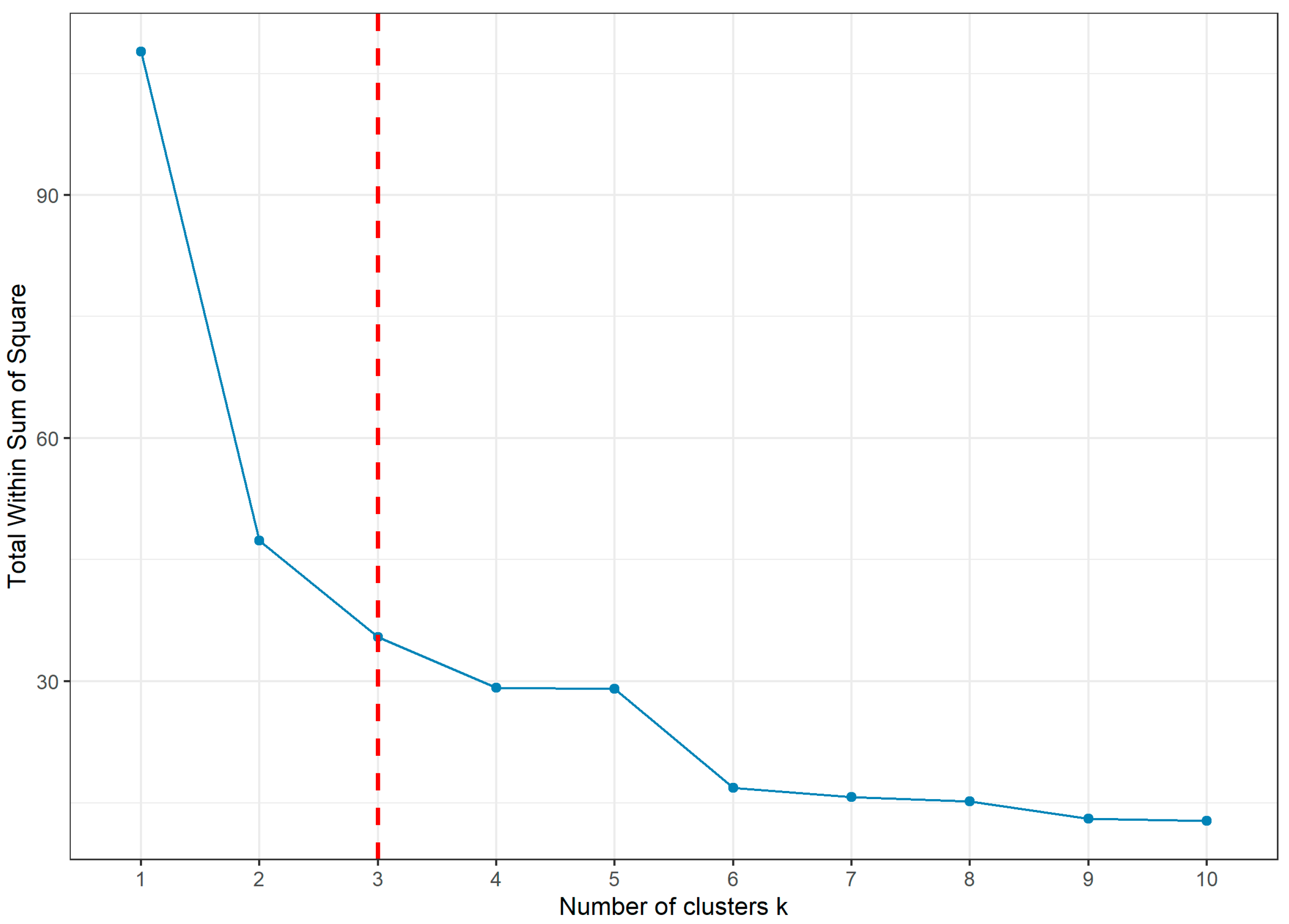
Figure 5.
5-NN distance plot for DBSCAN.
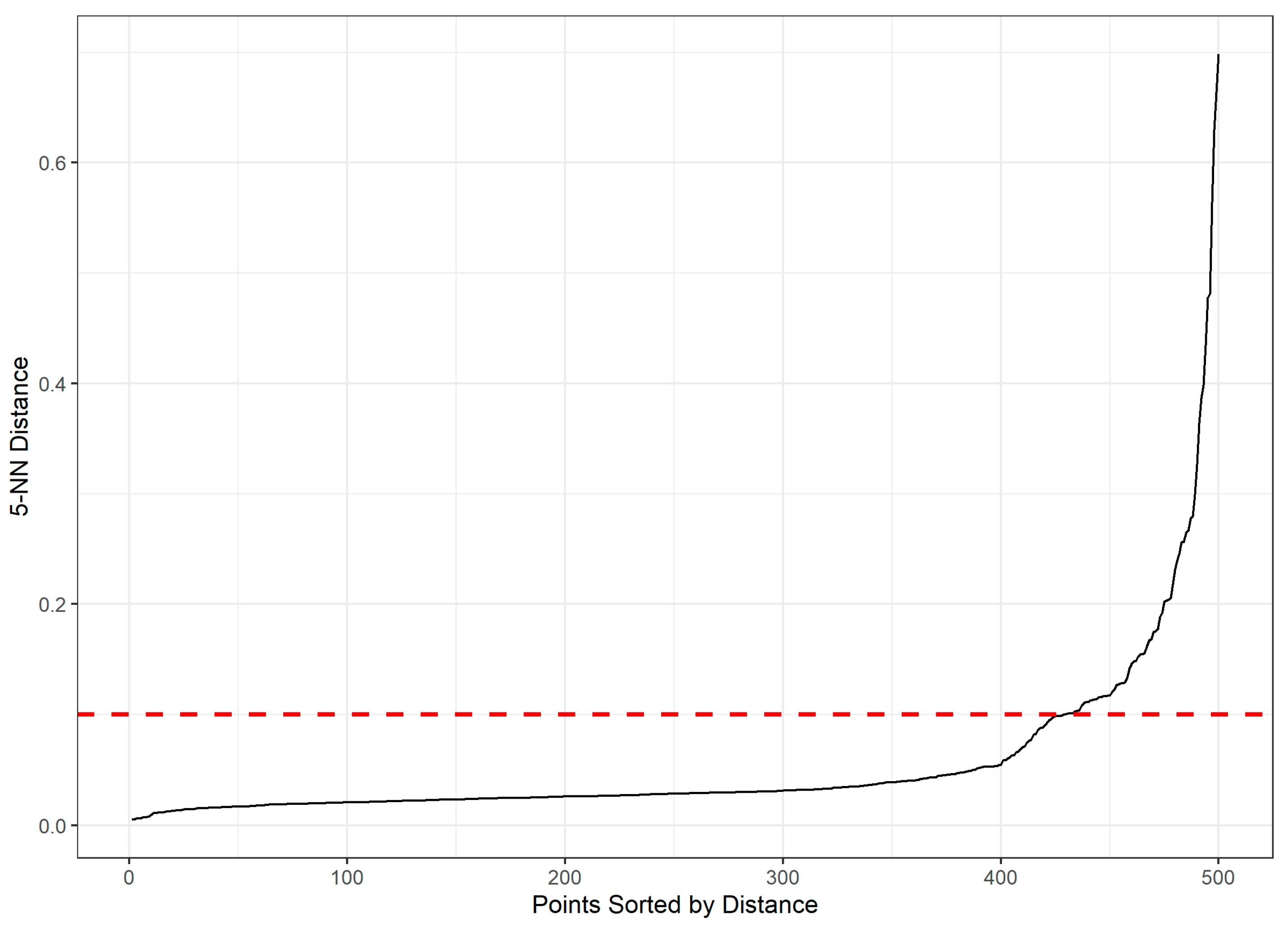
Figure 6.
BIC plot for GMM.
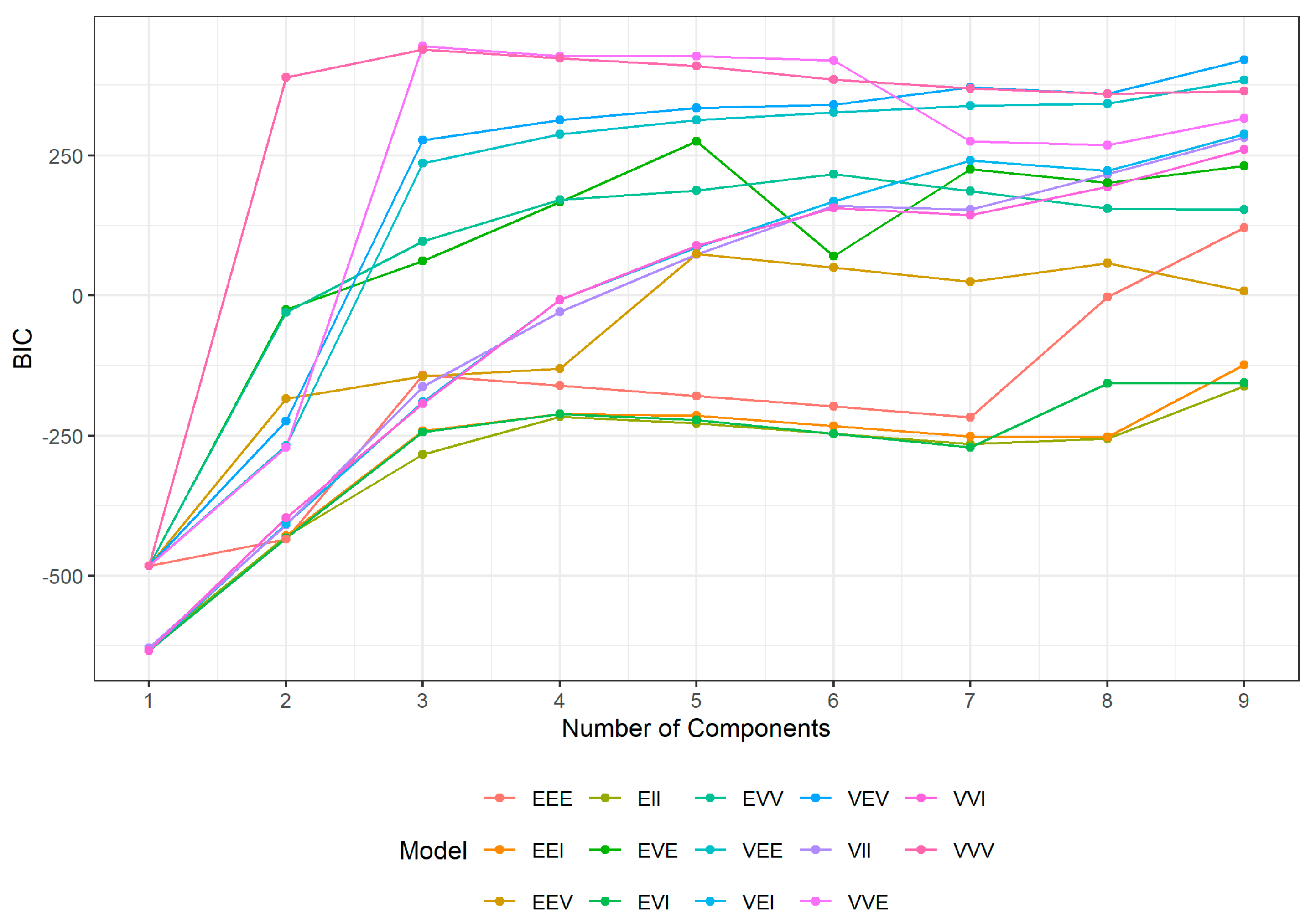
Figure 7.
FCM results: (a) Error space results; (b) Spatial distribution of clusters in the study area.
Figure 7.
FCM results: (a) Error space results; (b) Spatial distribution of clusters in the study area.
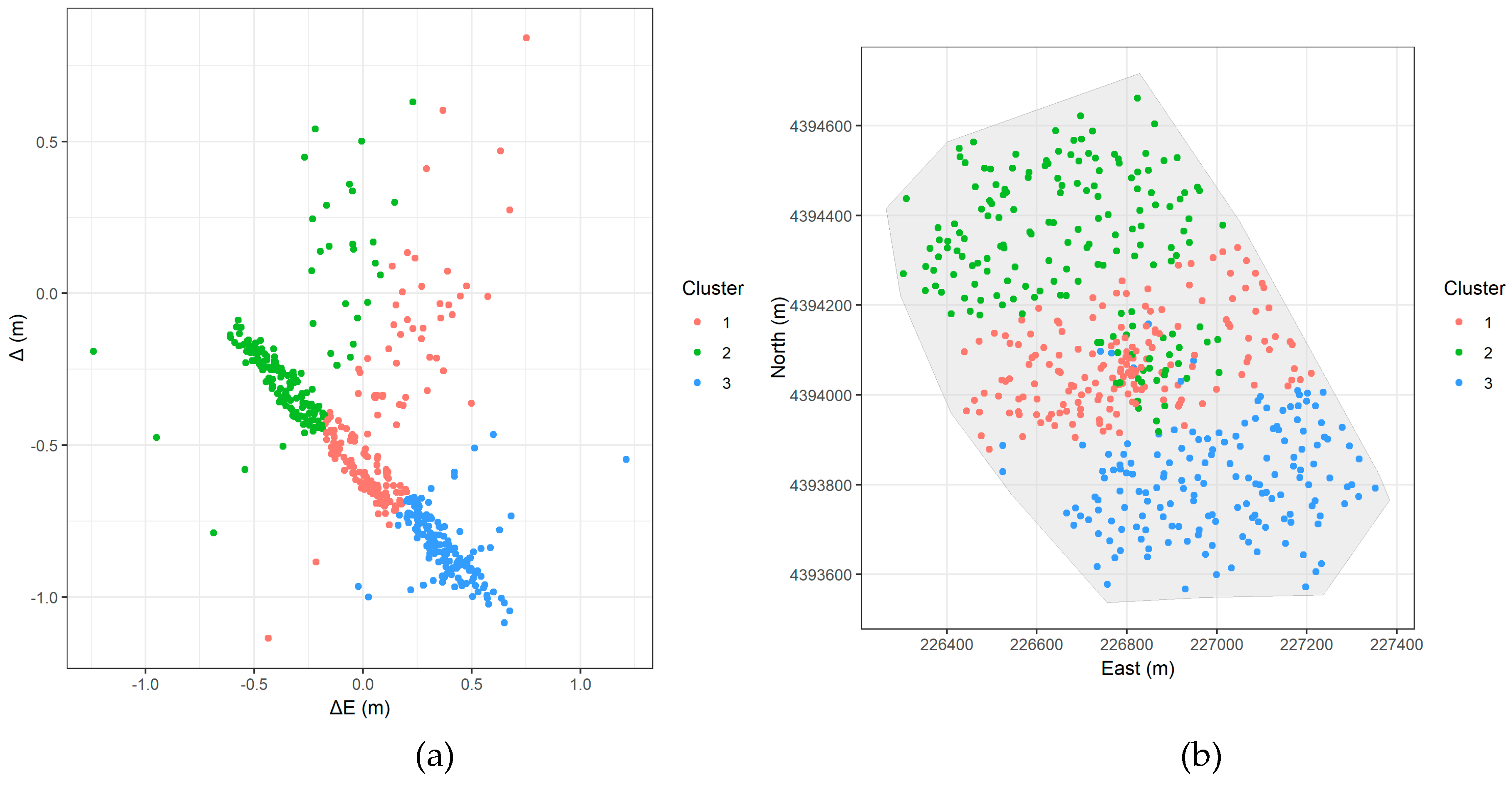
Figure 8.
DBSCAN results: (a) Error space results; (b) Spatial distribution of clusters in the study area.
Figure 8.
DBSCAN results: (a) Error space results; (b) Spatial distribution of clusters in the study area.
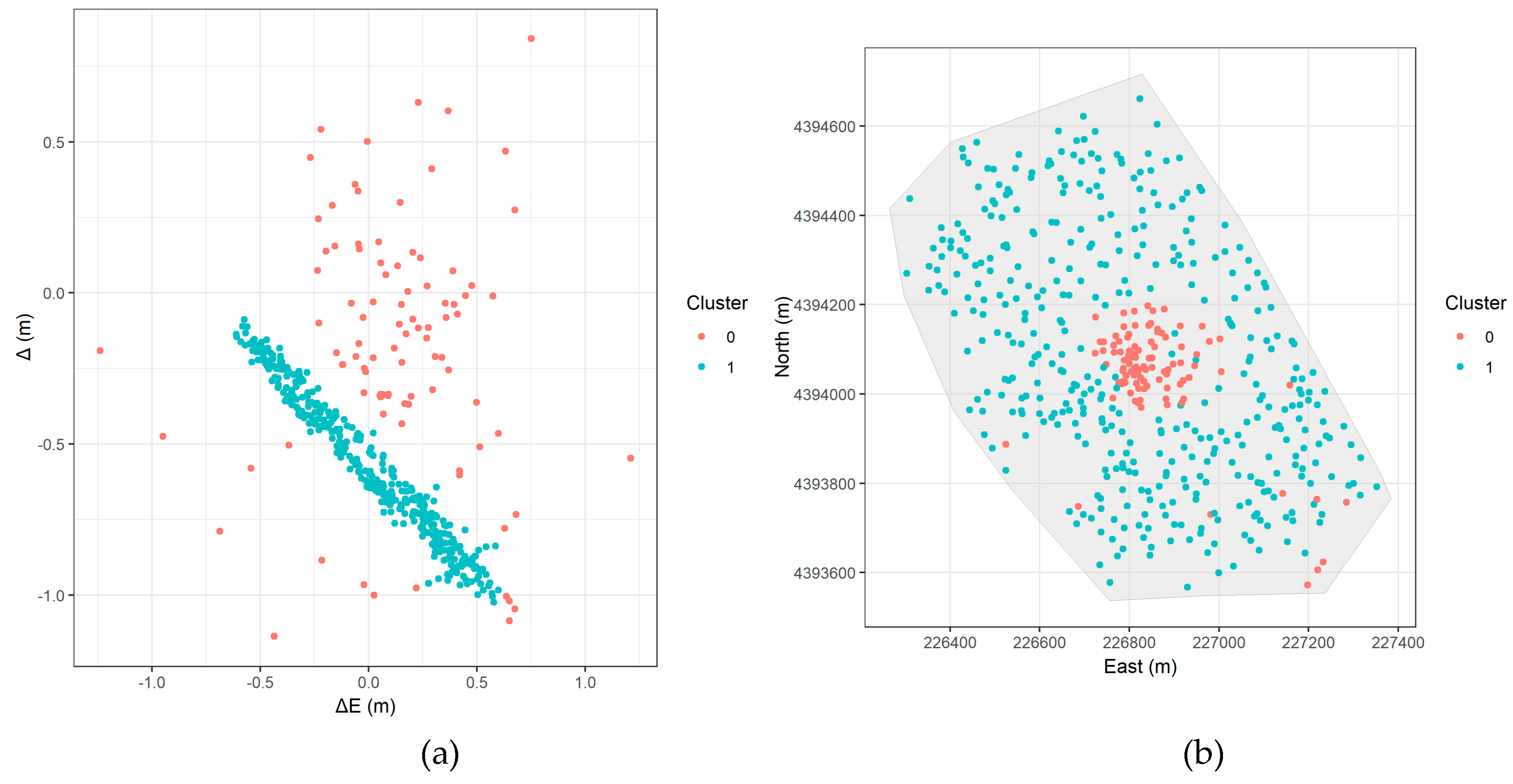
Figure 9.
GMM results: (a) Error space results; (b) Spatial distribution of clusters in the study area (actual space).
Figure 9.
GMM results: (a) Error space results; (b) Spatial distribution of clusters in the study area (actual space).


Table 1.
The average statistical properties of and and L values. SD is an abbreviation for standard deviation and CV for coefficient of variation (the absolute value of ratio of the standard deviation to the mean). All values except skew, kurtosis and CV are in meters.
Table 1.
The average statistical properties of and and L values. SD is an abbreviation for standard deviation and CV for coefficient of variation (the absolute value of ratio of the standard deviation to the mean). All values except skew, kurtosis and CV are in meters.
| Metric | Min | Mean | Median | Max | SD | Skew | Kurtosis | CV |
|---|---|---|---|---|---|---|---|---|
| ΔE | -0.95 | 0.03 | 0.05 | 1.21 | 0.33 | -0.06 | -0.65 | 10.67 |
| ΔN | -1.13 | -0.50 | -0.53 | 0.84 | 0.33 | 0.75 | 0.76 | 0.66 |
| L | 0.04 | 0.63 | 0.59 | 1.33 | 0.25 | 0.28 | -0.47 | 0.39 |
Table 2.
Mean Silhouette Scores (unitless) for Each Clustering Algorithm.
| Algorithm | Mean Silhouette Score |
|---|---|
| FCM | 0.43 |
| DBSCAN | 0.33 |
| GMM | 0.27 |
Table 3.
The average statistical properties of clusters. SD is an abbreviation for standard deviation.
Table 3.
The average statistical properties of clusters. SD is an abbreviation for standard deviation.
| Algorithm | Cluster | Number of Points | Mean ΔE (m) | Mean ΔN (m) | SD ΔE (m) | SD ΔN (m) | Mean Length (m) |
|---|---|---|---|---|---|---|---|
| FCM | 1 | 178 | -0.336 | -0.224 | 0.184 | 0.215 | 0.471 |
| 2 | 158 | 0.385 | -0.831 | 0.139 | 0.11 | 0.923 | |
| 3 | 164 | 0.068 | -0.462 | 0.169 | 0.262 | 0.537 | |
| DBSCAN | 0 (noise) | 102 | 0.088 | -0.172 | 0.366 | 0.387 | 0.47 |
| 1 | 398 | 0.008 | -0.576 | 0.332 | 0.246 | 0.678 | |
| GMM | 1 | 103 | 0.077 | -0.166 | 0.352 | 0.37 | 0.458 |
| 2 | 397 | 0.01 | -0.579 | 0.336 | 0.249 | 0.682 |
Disclaimer/Publisher’s Note: The statements, opinions and data contained in all publications are solely those of the individual author(s) and contributor(s) and not of MDPI and/or the editor(s). MDPI and/or the editor(s) disclaim responsibility for any injury to people or property resulting from any ideas, methods, instructions or products referred to in the content. |
© 2025 by the authors. Licensee MDPI, Basel, Switzerland. This article is an open access article distributed under the terms and conditions of the Creative Commons Attribution (CC BY) license (http://creativecommons.org/licenses/by/4.0/).
Copyright: This open access article is published under a Creative Commons CC BY 4.0 license, which permit the free download, distribution, and reuse, provided that the author and preprint are cited in any reuse.


