Comparative Study of Different Linear Analysis for Seismic Resistance of Buildings According to Eurocode 8

1. Introduction

The assessment of seismic resistance of buildings is very important on the stage of their design in order to prevent life losses in earthquake events. The methods of such an assessment are computational by modelling and applying the finite element method for analysis and simulation. The seismic loading can be presented in two ways [1]. One is by real accelerograms, recorded and scaled to the hazard level of design. The other one is to use the response spectrum as a generalized characteristic of the earthquake ground motion accounting for the hazard level.

The methods of seismic analysis are linear and nonlinear. The nonlinear methods aim to find the capacity of building structures to withstand plastic deformations in a seismic loading without collapse. In order to do such analysis, one should know the nonlinear behavior of all elements of the structure and the nonlinear model should represent that behavior with fidelity. Usually, the nonlinear analysis determines the capacity of the structure which is used in the linear analysis. In Eurocode 8 (EC8), the behavior factor, $q$, is used for such a characteristic [1].

The linear methods of analysis, described in EC8, are “Lateral force analysis” and “Modal response spectrum analysis”, which is pointed as a reference method [1]. The lateral force method uses two types of a distribution of the forces: a linear distribution in the form of an inverted triangle (proportional to the height) and proportional to the displacements of the first mode shape. Both distributions are not theoretically justified. The modal response spectrum method uses each separate mode response as a Single Degree of Freedom (SDOF) system response and then the total response is calculated by means of one of the methods: Square Root of Sum of Squares (SRSS), and Complete Quadratic Combination (CQC). All they are not theoretically justified.

The simulations of the structure behavior under seismic loadings by artificial accelerograms although using a linear-elastic model could reveal better the dynamic response of the structure as well as some problems with a torsional behavior [2]. The aim of this research is to compare different methods of finite element dynamic simulations with artificial accelerograms to the recommended linear methods of analysis, described in EC8. The dynamic simulations can be done by a direct explicit time integration of the differential equation of motion [3], by a direct implicit time integration method, or by a modal model of the structure and modal equations of motion time integration [4]. The time integration of equations of motion requires significant computational time and a powerful computer capability.

2. Methodology

2.1. Artificial Accelerograms

The artificial accelerogram should correspond to the response spectrum of the earthquake [5]. The generator of the accelerograms, which is used here, is an available MATLAB® script well described in [6]. The generation of the artificial accelerogram is based on the real records of accelerograms of the following earthquakes:

• ElCentro Earthquake (1940);
• Gebze Earthquake (1999);
• Mexico City Earthquake (1985).

The original records are scaled to the level of the maximum acceleration chosen as a reference and in this case, it is $a_g=0.15 g=1.4175$ m/${\mathrm{s}}^2$, using the coefficient of importance ${\gamma }_I=1.0$ for ordinary buildings. The response spectrum chosen is the elastic spectrum, which is recommended in EC8 for earthquake type 1, soil type C and damping ratio of response $\zeta =5\%$. The response spectrum parameters are given in Table 1.

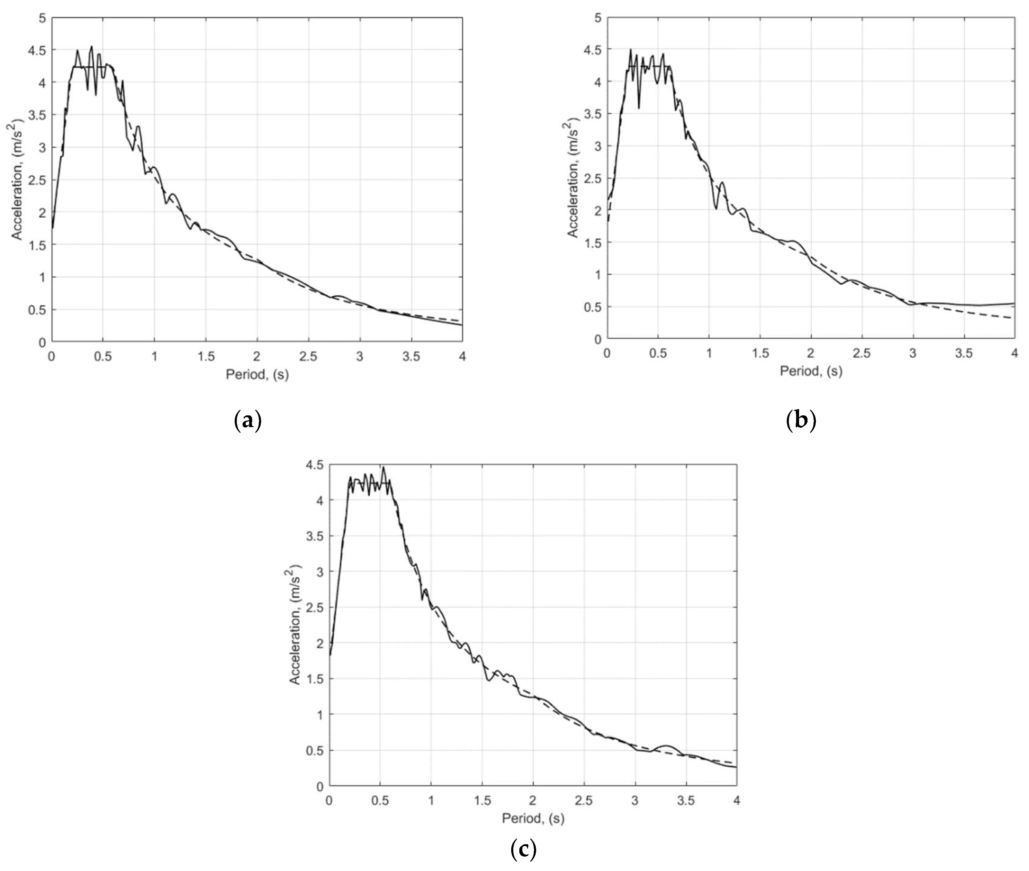
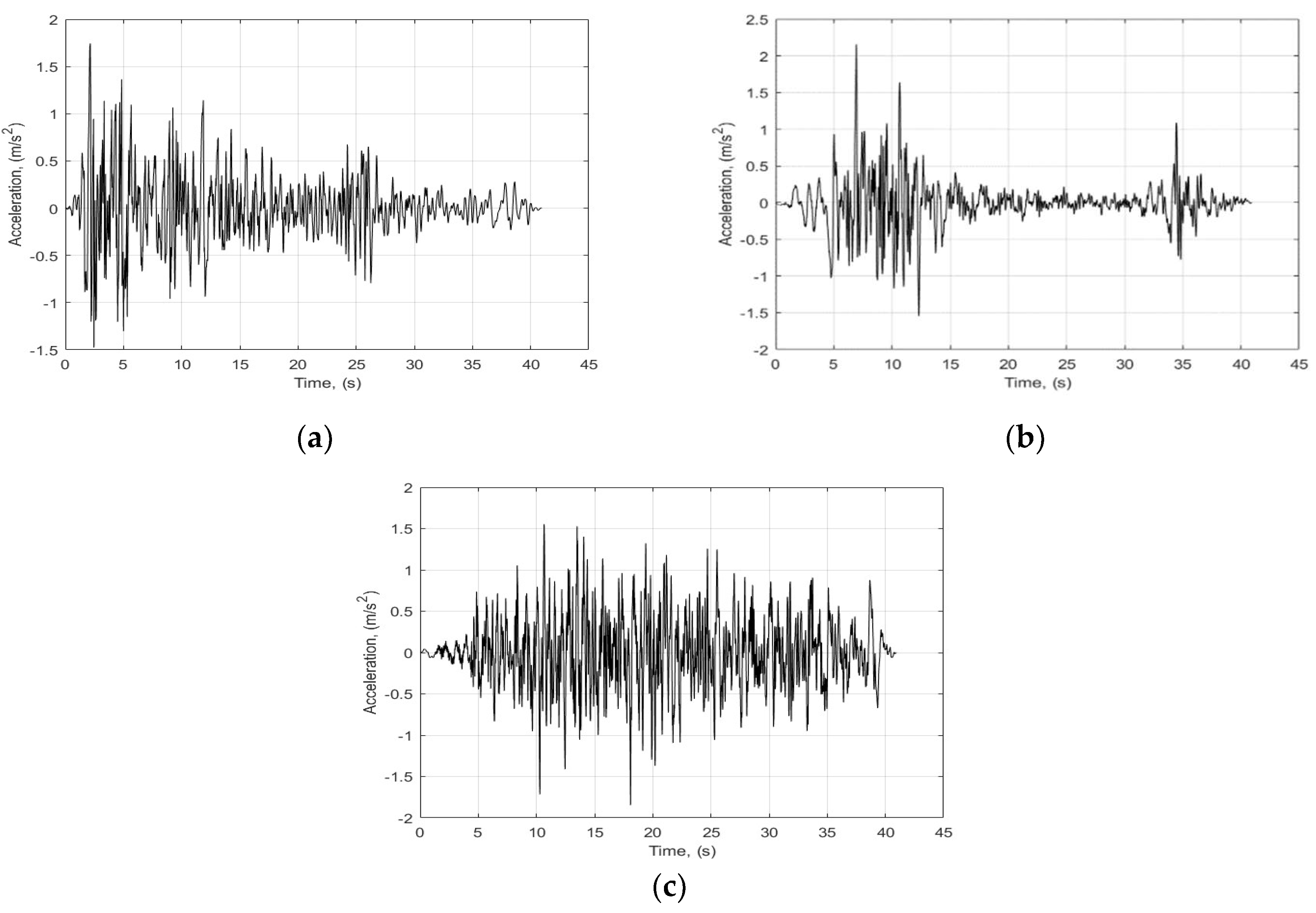
Three accelerograms are generated, corresponding to the earthquakes numbered above, and they are filtered in 8 iterations in order to be close to the chosen spectrum [6]. The correspondence of the generated accelerogram spectra to the reference spectrum can be seen in Figure 1. One can see that the artificial accelerograms are very good match for the response spectrum. The generated accelerogram are given in Figure 2. The time of accelerograms is trimmed at 40.96 s with a time step $\mathrm{d}t=0.005$ s which means 8192 points $=2^{13}$. The number of sample points should be some power of 2, in order the Fourier transformation to be done. When the accelerograms are generated, then the simulations of structure loading and response can be truncated up to any time less than 40.96 s. For the purpose of the structure dynamics simulations, the time of simulations is set to be 40 s and the number of sample points of the ground motion acceleration is $n_s=8000$.

2.2. Time-History Analysis

The solution of the dynamics of structure problem by accelerograms is found by direct time integration of the differential equation of motion for finite element model of the structure:

$$\mathbf{M}\ddot{\mathit{d}}+\mathbf{C}\dot{\mathit{d}}+\mathbf{K}\mathit{d}=\mathit{f},$$

(1)

where M, C, and K are the mass, the damping, and the stiffness matrices, respectively. The nodal displacements, $\mathit{d}$, are the unknowns as a function of time, $t$, while the external nodal force vector, $\mathit{f}$, is the inertia force vector, which components are:

$$f_i=r_i m_{i}a\left(t\right) , i=\mathrm{1,2}, \dots , N_{\mathrm{D}\mathrm{o}\mathrm{F}}$$

(2)

where $r_i$ is 1, if it is in the direction of seismic loading or 0 otherwise. Here $m_i$ is the lumped translational nodal mass and $a\left(t\right)$ is the acceleration at time, $t$, taken from the accelerogram, $N_{DoF}$ is the number of the Degrees of Freedom (DoF) of the finite element model of the structure.

2.2.1. Implicit Time Integration Method

The time domain is discretized in time steps, $\mathsf{\Delta }t$, and (1) holds at any time $t_n$ for step number $n$. There are two methods of time integration of (1): implicit and explicit. The implicit time integration can be expressed in this way:

$${\mathit{d}}_{n+1}=f({\dot{\mathit{d}}}_{n+1},{\ddot{\mathit{d}}}_{n+1}{,\mathit{d}}_n,\dots )$$

(3)

which should be read as find the displacements at $n+1$ time step as a function of the velocity and acceleration at the same time step plus all that is known from previous steps. The implicit method is unconditionally stable, so the time step, $\mathsf{\Delta }t$, could be any, but small enough in order to capture the dynamics of the structure. This is why we will solve the equation of motion with implicit method in 8000 increments (time steps). The great problem of the method is that a system of linear equations should be solved at each time step or iteration, which is time consuming calculations especially for large model with a lot of DoF.

2.2.2. Explicit Time Integration Method

The explicit method of time integration can be summarized in this way:

$${\mathit{d}}_{n+1}=f({\mathit{d}}_n,{\dot{\mathit{d}}}_n,{\ddot{\mathit{d}}}_n,{\mathit{d}}_{n-1},\dots )$$

(4)

Using lumped mass matrix and lagging the velocity in a half step behind leads to that all internal and viscous forces depending of displacements and velocities are known from the previous time steps, and only nodal accelerations should be determined for the current time step, ${\ddot{\mathit{d}}}_{n+1}$, then it is easy to find the velocities, ${\dot{\mathit{d}}}_{n+1/2}={\dot{\mathit{d}}}_{n-1/2}+\mathsf{\Delta }t {\ddot{\mathit{d}}}_{n+1}$, and the displacements, ${\mathit{d}}_{n+1}={\mathit{d}}_n+\mathsf{\Delta }t {\dot{\mathit{d}}}_{n+1/2}$, node by node. The solution of the equation of motion in the time steps consists of nodewise and elementwise cycles of calculations without any linear equation system solution. This makes time step calculations very fast and efficient, however the method is conditionally stable.

The condition for stability of the time integration is that the time step should be:

$$\mathsf{\Delta }t\le {\displaystyle \frac{2}{{\omega }_{\mathrm{m}\mathrm{a}\mathrm{x}}}} , {\omega }_{\mathrm{m}\mathrm{a}\mathrm{x}}={\displaystyle \frac{2c}{L_{\mathrm{m}\mathrm{i}\mathrm{n}}}}$$

(5)

where ${\omega }_{\mathrm{m}\mathrm{a}\mathrm{x}}$ is the maximum angular frequency of the discretized structure, which is determined by the element with a high sound speed, $c$, and a small minimal distance between its nodes, $L_{\mathrm{m}\mathrm{i}\mathrm{n}}$. This condition depends on the degree of discretization of the structure and makes the time step very small. The problem is solved on the level of tracking mechanical waves, which means it makes real life simulations of mechanical interactions and dynamics.

The number of increments in time could be very high. When it is comparatively small as in case of very short transient events as impact simulations or explosion simulations, a single precision is used in the computer calculations, which makes the problem solution quite acceptable. However, for time of event as 40 s, that we have for time-history analysis, double precision calculations are necessary in order to avoid the error accumulation with the large number of increments.

2.2.3. Modal Transient Dynamics

The other method of time-history analysis is to establish a modal numerical model of the structure and to solve the modal dynamics equation of motion [4]. The mode shapes ${\mathit{\varphi }}_i$ are the solution of the free vibration equation of motion:

$$\left(\mathbf{K}-{\lambda }_i\mathbf{M}\right){\mathit{\varphi }}_i=\mathit{O}$$

(6)

where ${\lambda }_i={\omega }_i^2$ are the eigen values, corresponding to the natural angular frequencies ${\omega }_i$, which are the solution of the algebraic equation:

$$\mathrm{d}\mathrm{e}\mathrm{t}\left(\mathbf{K}-\lambda \mathbf{M}\right)=0$$

(7)

Using the modal matrix $\mathsf{\Phi }=\left[\begin{array}{cccc}{\mathit{\varphi }}_1& {\mathit{\varphi }}_2& \cdots & {\mathit{\varphi }}_n\end{array}\right]$ to present the displacements $\mathit{d}=\mathsf{\Phi }\mathit{z}\left(t\right)$, the matrix equation of motion becomes a set of independent modal equations due to the orthogonality of the mode shapes, ${\mathit{\varphi }}_j$:

$${\overline{M}}_j{\ddot{z}}_j\left(t\right)+{\overline{C}}_j{\dot{z}}_j\left(t\right)+{\overline{K}}_j{z}_j\left(t\right)=y_j\left(t\right) , j=\mathrm{1,2},\dots , n$$

(8)

where ${\overline{M}}_j$, ${\overline{C}}_j$, and ${\overline{K}}_j$ are the modal mass, the modal viscous damping coefficient, and the modal stiffness coefficient, respectively. The modal force $y_j={\sum }_{i=1}^{N_{DoF}}{\varphi }_{ij}{f}_i$ is obtained from inertia nodal forces $f_i$ in seismic loading given by (2). The scalar ${\varphi }_{ij}$ is the $i,j$ component of the modal matrix $\mathsf{\Phi }$. The great advantage of the modal method is that the number of modes, $n$, used to represent the dynamic motion of the structure, can be very small, because it is dominated by the very low frequency mode shapes. According to the EC8 the modal model should include all modes with the accumulated participation of effective modal masses at least 90% of the total mass of the structure in each direction of seismic loadings and modes with more than 5% of the mass participation.

Because the truncation of modes leads to loss of masses, some methods are proposed to compensate the missing mass [7]. According to [8] the most efficient method however is to add the residual mode [9]. This additional improvement of the modal model of the structure will be examined for all modal solutions.

2.3. Response Spectrum Analysis

2.3.1. Lateral Force Method for Static Loading

Eurocode 8 recommends two linear-elastic solutions using the response spectrum. The first one is the lateral force method, where the structure is considered as a SDOF system, and the total base shear force is calculated from the response spectrum in this way:

$$F_b=S_d\left(T_1\right) m \lambda$$

(9)

where $S_d$ is a design spectrum pseudo acceleration corresponding to the fundamental period of vibration, $T_1$, in the direction of loading considered, $m$ is the total mass of the structure, and $\lambda =0.85$ if $T_1\le 2 T_C$ and the building has more than 2 stories, otherwise $\lambda =1.0$. Here, an elastic response spectrum with 5% damping is used instead of a design response spectrum because the artificial accelerograms are generated for the elastic response spectrum.

The base shear force is distributed as story forces acting on each floor in one of the two ways. One way is to distribute the force proportional to the story mass, $m_i$, and fundamental modal displacements, $s_i$:

$$F_i=F_b{\displaystyle \frac{s_i{m}_i}{{\sum }_{j=1}^k{s}_j{m}_j}}$$

(10)

where $F_i$ is the story force, and the number of stories is $k$. The other way is to distribute the force proportional to the floor height $z_i$ and story mass $m_i$:

$$F_i=F_b{\displaystyle \frac{z_i{m}_i}{{\sum }_{j=1}^k{z}_j{m}_j}}$$

(11)

The lateral force method is a static analysis method when the structure is loaded by those story forces.

2.3.2. Modal Response Spectrum Analysis

The Modal response spectrum method uses the modal equations (7), where instead of functions of time, we have the maximal response, which means the modal force becomes:

$$y_j={\overline{L}}_j{S}_{dj}\left(T_j\right) , j=\mathrm{1,2},\dots , n$$

(12)

where $S_{dj}\left(T_j\right)$ is the design response spectrum pseudo acceleration for a modal period $T_j$ and ${\overline{L}}_j$ is the coefficient of mass participation in the direction of motion:

$${\overline{L}}_j=\sum _{i=1}^{N_{DoF}}{m}_i{\varphi }_{ij}{r}_i , j=\mathrm{1,2},\dots , n$$

(13)

where $m_i$ is the node mass and $r_i$ is unity if $i-$DoF is in the direction of the seismic loading and zero otherwise. Introducing the modal mass ${\overline{M}}_j$ as:

$${\overline{M}}_j=\sum _{i=1}^{N_{DoF}}{m}_i{\varphi }_{ij}^2 , j=\mathrm{1,2},\dots , n$$

(14)

the modal participation factor of mode $j$ in the motion of loading direction, ${\overline{\mathsf{\Gamma }}}_j$, is defined:

$${\overline{\mathsf{\Gamma }}}_j={\displaystyle \frac{{\overline{L}}_j}{{\overline{M}}_j}} , j=\mathrm{1,2},\dots , n$$

(15)

The modal participation factor allows the maximum response as a modal acceleration, ${\ddot{z}}_j$, to be determined, ignoring the damping and elastic forces in the equation:

$${\ddot{z}}_j\left(\mathrm{m}\mathrm{a}\mathrm{x}\right)={\overline{\mathsf{\Gamma }}}_j{S}_{dj}\left(T_j\right) , j=\mathrm{1,2},\dots , n$$

(16)

Using the modal matrix $\mathsf{\Phi }$, the maximum acceleration of any DoF $i$ as a response to any mode $j$ can be determined:

$${\ddot{d}}_{ij}\left(\mathrm{m}\mathrm{a}\mathrm{x}\right)={\overline{\mathsf{\Gamma }}}_j{S}_{dj}\left(T_j\right){\varphi }_{ij} , i=\mathrm{1,2},\dots , N_{DoF} , j=\mathrm{1,2},\dots , n$$

(17)

or the maximum displacement of the $i$-th DoF to the $j$-th mode:

$$d_{ij}\left(\mathrm{m}\mathrm{a}\mathrm{x}\right)={\overline{\mathsf{\Gamma }}}_j{S}_{dj}\left(T_j\right){\varphi }_{ij}{\left({\displaystyle \frac{T_j}{2\pi }}\right)}^2 , i=\mathrm{1,2},\dots , N_{DoF} , j=\mathrm{1,2},\dots , n$$

(18)

Instead of the design response spectrum $S_d$ in (12, 17, and 18), the elastic response spectrum with 5% damping is used. Based on the maximum displacements determined above, any nodal effect, $E_{ij}$, due to the $j$-th mode as section forces and moments as well as stresses can be determined. The combination of them should be done by SRSS method:

$$E_i=\sqrt{{\sum }_{j=1}^n{E}_{ij}^2} , i=\mathrm{1,2},\dots ,N_{DoF}$$

(19)

according to the EC8, and if the natural frequencies of two modes are close enough, then the method of CQC is recommended:

$$E_i=\sqrt{{\sum }_{k=1}^n{\sum }_{j=1}^n{E}_{ij}{\rho }_{jk}{E}_{ik}} , i=\mathrm{1,2},\dots , N_{DoF}$$

(20)

where

$${\rho }_{jk}={\displaystyle \frac{8\sqrt{{\zeta }_j{\zeta }_k}\left({\zeta }_j+r{\zeta }_k\right)r^{3/2}}{{\left(1-r^2\right)}^2+4{\zeta }_j{\zeta }_{k}r\left(1+r^2\right)+4\left({\zeta }_j^2+{\zeta }_k^2\right)r^2}} , r={\displaystyle \frac{{\omega }_k}{{\omega }_j}}$$

(21)

Some investigations show that the CQC method is supreme over the SRSS method [10].

3. Structure Model

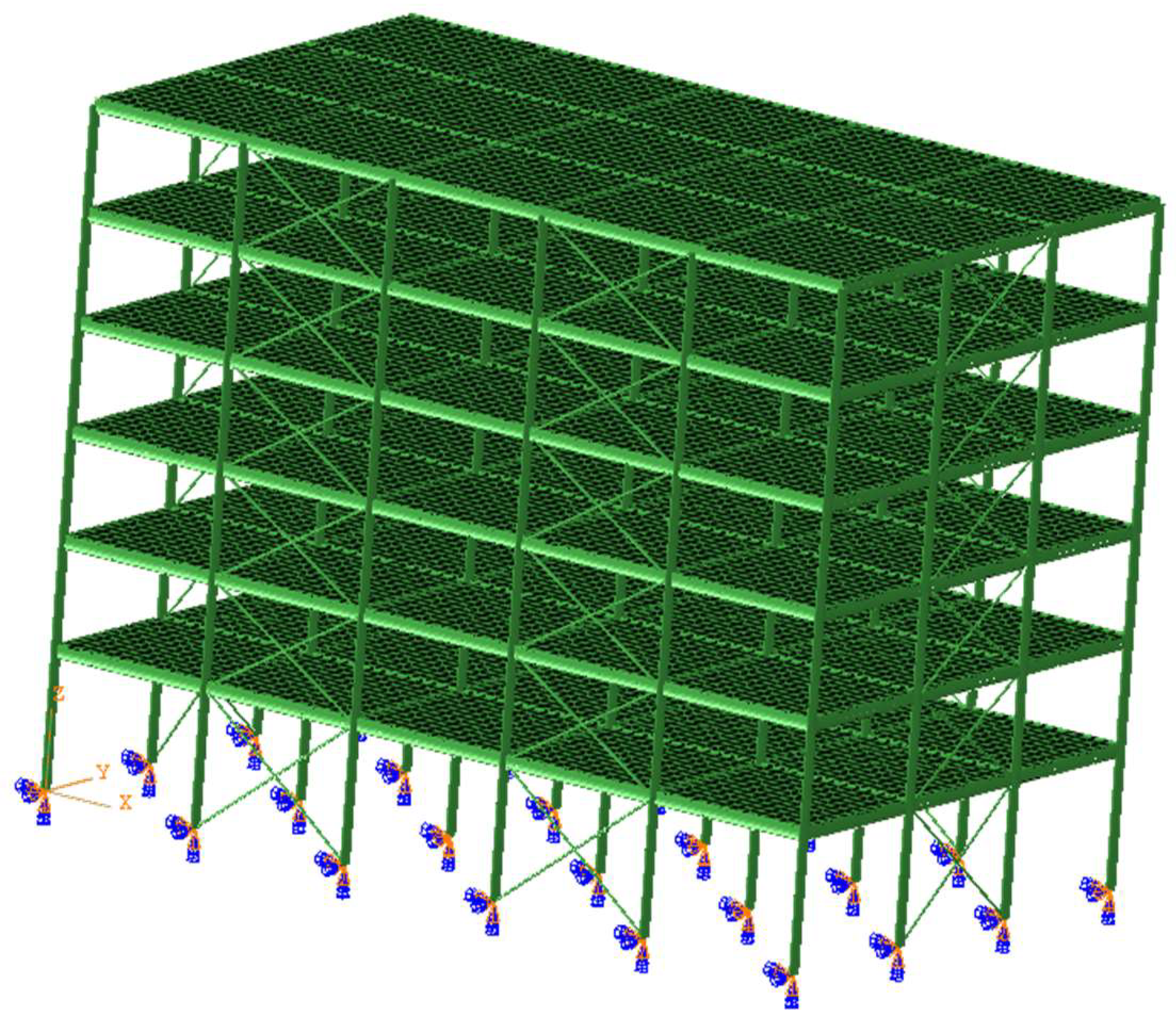
The example structure, which is examined under seismic loadings, is steel structure of a 6-story building. The finite element model of the structure in SIMULIA Abaqus® is given in Figure 3. It consists of 3 792 beam elements, 72 truss elements, and 12 960 shell elements or totally 16 824 elements, 22 062 nodes, and 86 868 variables or $N_{DoF}$.

The structure has 6 columns in X-direction and 4 columns in Y-direction or totally 24 columns of standard steel profile HE 500A (EN 10365: 2017). The strong axis of column profiles is oriented in X-direction. All girders are standard steel profile IPE 450 (EN 10365: 2017). The girders have their strong axis in Y-direction, if they have their longitudinal axis in X-direction and vise verses. The structure is braced by truss elements corresponding to standard steel profile UPN 120 (EN 10365: 2017). The geometric characteristics of profiles, necessary for their finite element section descriptions are given in Table 2. The elastic modulus of steel is $E=210 \mathrm{G}\mathrm{P}\mathrm{a}$, Poisson’s ratio is $\nu =0.3$, and material density is $\rho =7.85 \mathrm{t}/{\mathrm{m}}^3$.

The floor plates are modelled by shell elements having thickness of 20 cm, Young’s modulus $E=50 \mathrm{G}\mathrm{P}\mathrm{a}$, Poisson’s ratio $\nu =0.2$, and density $\rho =2.5 \mathrm{t}/{\mathrm{m}}^3$, which is close to a homogenized reinforced concrete plate. All elements have a preferable discretization size of 0.5 m and shell elements and beam elements have common nodes. The distance between the columns is 6 m in both directions, the height of the first story is 4.5 m and the distance between stories is 3.5 m. The structure is 30 m long in X-direction, 18 m wide in Y-direction, and 22 m high in Z-direction. All columns are fixed in their base.

4. Results and Discussion

The numerical examples using different methods of analysis are run on a work station computer having 2 processors Intel Xeon E5-1660 v4 @ 3.20 GHz, 8 cores each, but all solutions required 8 cores for the calculations. The natural frequency and mode shape analysis shows close first and second frequencies and that first 5 modes are enough to satisfy requirements for the effective modal mass participation as can be seen in Table 3, because the structure mass is calculated as 1 814.7 tones.

The effects of all seismic loading analysis, that are observed, are as follows: the total reaction at the base of columns in the direction of seismic loading, $R_{tot}$; maximum displacement, $d_{max}$; maximum von Misses stress in columns, ${\sigma }_{col}$; maximum von Misses stress in girders, ${\sigma }_{gir}$; and maximum von Misses stress in diagonal bars (truss elements), ${\sigma }_{bar}$;. The effects of seismic loadings to the plates are small, so they are ignored here. The total reaction could not be calculated for modal response spectrum method. The results for the modal response spectrum method, are given in Table 4.

The results show that there is almost no difference between model with only 5 modes and the model with 5 modes plus the residual mode. The difference between methods of gathering the effects of different modes is nothing although according to EC8 when the one frequency is higher than 90% of the next frequency, the CQC method should be applied, instead of the SRSS method, because they are very close frequencies, and the SRSS method is not appropriate.

Applying the lateral force method, the story masses are assumed to be equal, which means they are ignored in (10) and (11). The base total shear force is calculated for X-direction by the first mode natural frequency, 1.2459 Hz, and this results in $F_{bX}=4878$ kN, while in Y-direction, using the second natural frequency, 1.3647 Hz, the base shear force is $F_{bY}=5343$ kN.

The results for lateral force method are given in Table 5. The difference between the ways of distribution of the total base shear force over the stories is comparatively small. There is a difference between the modal response spectrum solution and the lateral force method. The difference however is not more than 4% and it is higher when the loading is in X-direction, in which direction the structure is stiffer.

The time-history simulations of seismic loading by accelerograms should be done in the same conditions as response spectrum methods, which means with the same damping ratio $\zeta =5$%. In order to do that, damping by Rayleigh is assumed, which is determined by the formula:

$$\zeta ={\displaystyle \frac{\alpha }{2{\omega }_1 }}+{\displaystyle \frac{\beta {\omega }_1}{2}}$$

(22)

where ${\omega }_1=2\pi f_1$ is the fundamental angular frequency of the structure and it is assumed that $\beta =0$. The obtained value for $\alpha$ is $\alpha =0.78282$.

The simulations are run for a 40 s problem time and 2 000 states are recorded. The implicit method of simulations as well as the modal dynamics method have 8 000 increments with fixed time step, while the explicit method has 2 143 928 increments. The wall-clock time for running the time-history analysis using different accelerograms is given in Table 6 in seconds.

The fastest analysis is the modal dynamics analysis which has approximately 18 minutes for running, but this method is linear-elastic by origin. The explicit analysis is running for approximately 1 hour and 40 minutes, which is quite longer, but the method can be totally nonlinear, because it is on the level of sound wave tracking. The implicit time-history analysis has time for running approximately 1 hour and 25 minutes. This is not very different than explicit simulations, because the building frame structures are very simple with relatively few DoF and high critical time step, where the explicit analysis has better performance, although it runs in double precision calculations.

The results for the effects of seismic loading for the different time-history analysis are given in Table 7. The first expression is that there is quite different response to the different accelerograms. Another issue is that the implicit, and the modal transient simulations show a little bit higher values, compared with the explicit analysis and the values of modal dynamics method with 6 modes (5 modes + residual mode) in X-direction are significantly higher.

The effects of the accelerogram #2 simulations are highest and let compare them to the other two accelerogram response. Taking as a reference the second accelerogram effects the relative divergency for explicit analysis is calculated and shown in Table 8. The relative divergency is calculated in percent by formula:

$$relative divergency={\displaystyle \frac{reference value-relative value}{reference value }} 100 \%$$

(23)

The results in Table 8 show a comparatively great divergency of the dynamic response of the structure to the accelerograms. The greatest one is 16.5 %. Let compare the different methods for time-history analysis to the explicit method by calculating the relative divergency only for an accelerogram #2. The results are given in Table 9.

The results in Table 9 show that all methods for time-history analysis have a comparatively close assessment of the effects of seismic loadings. The positive divergency is maximum 1.4 % and a negative divergency means overestimated values, which maximum is 6.4 %, but it is on the side of safety.

From safety point of view, the highest dynamic response of the structure to the accelerograms should be taken as a basis for design. The assessment of effectiveness of response spectrum method is done by calculating the relative divergency of the effects of seismic loading compared to explicit analysis using accelerogram #2. The results are given in Table 10.

The analysis of data in Table 10 shows that the response spectrum methods can give us approximately 10 % underestimation of seismic effects to the structure and especially to the weak direction of the structure. The modal response spectrum method can run for a few seconds but it is not so conservative, as it is believed. The structure should be examined even by more artificial accelerograms in order to find the maximum response and to reveal its behavior.

5. Conclusions

The different representations of seismic loading show some differences in the effects of that loading. Although the artificial accelerograms are pointed as alternative representation of seismic loadings to the response spectrum, they could become an essential part of the analysis for seismic resistance of building structures in the stage of their design. The following conclusions can be drawn:

• The artificial accelerograms, although having very similar spectra, have a great diversity to the dynamic response of structures and to the effects of loadings. Looking for the maximum response and effects, it is necessary to try more than the minimum requirement of three accelerograms in one direction;
• All methods for time-history analysis have similar results, and the fastest and the cheapest method is the modal transient dynamic method, which however is only linear method of analysis. However, when nonlinear simulations with accelerograms are needed the explicit time integration method is superior and it is not so expensive, because the building frame structure model have relatively few DoF and high critical time step, so itd can be easily calculated even with a double precision;
• The response spectrum methods are very fast and easy for calculations. However, they are not so conservative. Compared with time-history analysis methods, they can underestimate the effects of seismic loadings with approximately 10 %.

References

- European Committee for Standardization. EN 1998-1 Eurocode 8: Design of Structures for Earthquake Resistance – Part 1: General Rules, Seismic Actions and Rules for Buildings. European Committee for Standardization, Brussels, Belgium, 2004; pp. 33-76.
- Bommer, J.J.; Stafford, P.J. Seismic hazard and earthquake actions. In Seismic Design of Buildings to Eurocode 8, 2nd ed.; Elghazouli, A.Y., CRC Press, Taylor & Francis, Boca Raton, FL, 2017, pp. 7-40.
- Wu, S.R.; Gu, L. Introduction to the explicit finite element method for nonlinear transient dynamics, John Wiley & Sons, Inc., Hoboken, New Jersey, USA, 2012.
- Petyt, M. Introduction to finite element vibration analysis, 2-nd edition, Cambridge University Press, New York, USA, 2010; pp.367-412.
- Iervolino, I.; De Luca, F.; Cosenza, E. Spectral shape-based assessment of SDOF nonlinear response to real, adjusted and artificial accelerograms. Eng Struct. 2010, 32, 2776–2792. [Google Scholar]
- Ferreira F, Moutinho C, Cunha Á, Caetano E. An artificial accelerogram generator code written in Matlab. Eng. Rep. 2020;2:e12129. [CrossRef]
- Chopra, AK. Dynamics of structures: theory and applications to earthquake engineering. 4-th edition, New Delhi: Prentice-Hall of India; 2005.
- Dhileep, M.; Bose, P.R. A comparative study of ‘‘missing mass” correction methods for response spectrum method of seismic analysis, Comp. and Struct. 2008, 86, 2087–2094. [Google Scholar] [CrossRef]
- Salmonte, A.J. Considerations on the residual contribution in modal analysis. Earthq. Eng. & Struc. Dyn. 1982, 10, 295–304. [Google Scholar]
- Wilson, E.L.; Der Kiureghian, A.; Bayo, E.P. A replacement for the srss method in seismic analysis. Earthq. Eng. & Struc. Dyn. 1981, 9, 187–192. [Google Scholar]