
Submitted:
22 March 2025
Posted:
24 March 2025
You are already at the latest version
Abstract
It is evident that earthquakes can turn into disasters if buildings in affected areas are constructed without proper engineering. The February 6, 2023, Kahramanmaraş earthquakes of Türkiye impacted 14 million people across 11 cities and caused over 150 billion USD in damage. Assessing the structural safety of existing buildings is crucial to reducing earthquake risks. In this study, first phase of seismic risk assessment for an educational building in Yakutiye, Erzurum was conducted. Data was collected, a finite element model was created, and a theoretical modal analysis was performed. The theoretical fundamental vibration period of 1.220 seconds for the four-story structure was found to be high. To verify this, a dynamic identification study was carried out. Operational modal analysis, including sensor optimization, determined the in-situ fundamental vibration period as 0.241 seconds. The additional rooftop floor significantly affected the building’s modal behavior. The discrepancy between theoretical and experimental values was due to the omission of infill wall stiffness in the finite element model. Neglecting infill wall effects in seismic risk assessments may lead to incorrect results, underestimating seismic forces. The study found that the building could experience earthquake forces ~5 times higher than that of the theoretical estimation.
Keywords:
earthquake
; seismic risk assessment
; theoretical modal analysis
; operational modal analysis
; sensor optimization
; infill wall stiffness
1. Introduction
An earthquake is a natural phenomenon. It is possible to state that most of the earthquakes, which can be classified into different groups based on their formation, are tectonic earthquakes. Every day, earthquakes of varying magnitudes occur around the world. In 2024 alone, 1,374 earthquakes with a magnitude of 5 and above were recorded globally, while in 2023, the number was 1,780, including the catastrophic Kahramanmaraş earthquakes of February 6, 2023 [1]. The statistics of 2023 notably includes the earthquakes in Türkiye, which had an undeniable numerical contribution to the global total. According to the data from the Turkish Ministry of Interior Disaster and Emergency Management Authority, 62 earthquakes with a magnitude of 5 and above occurred in Türkiye in 2023, while in 2024, there were 7 such earthquakes [2]. The distribution of earthquakes with a magnitude of 5 and above in the Anatolian Peninsula in 2023 and 2024 is shown on the map in Figure 1.
The earthquake distributions shown in Figure 1 are displayed on the Earthquake Hazard Map of Türkiye. It is clearly observed that earthquakes are concentrated along the North Anatolian Fault Zone and East Anatolian Fault Zone. It can be stated that 3.5% of the 5 and above magnitude earthquakes recorded worldwide in 2023 occurred on Turkish land. As two of the world’s most active earthquake zones, these fault lines have been the sites of devastating earthquakes in the last 40 years. Earthquakes such as the 1992 Erzincan, 1998 Adana, 1999 Kocaeli and Düzce, 2003 Bingöl, 2011 Van, 2020 Elazığ, and İzmir are historic events that resulted in thousands of fatalities and enormous economic losses that cannot yet be fully quantified. These generally 6+ magnitude earthquakes culminated in the Kahramanmaraş earthquakes on February 6, 2023, which affected a 1.2 million square kilometre area, including Lebanon, Egypt, Iraq, Iran, and Syria, and caused unprecedented destruction in history. On February 6, 2023, Türkiye experienced the "Great Disaster of the Century" with two earthquakes of 7.7 and 7.6 magnitudes, occurring at 04:17 and 13:24, respectively. These earthquakes affected 11 cities and over 14 million citizens, leading to more than 50,000 casualties and making over 850,000 residential units uninhabitable [3]. The destruction caused by the Kahramanmaraş earthquakes of February 6, 2023, was the largest in the history of the Republic of Türkiye and was observed to be several times more intense than the 1939 Erzincan and 1999 Kocaeli-Düzce earthquakes. The seismic intensity along the Adıyaman-Antakya line was recorded as X-XI on the Modified Mercalli Intensity Scale, with the maximum ground acceleration recorded at 1.62g at a station in Fevzipaşa (Islahiye) [4]. Various sources have estimated the direct and indirect material losses from the Kahramanmaraş earthquakes of February 6, 2023, in Türkiye to exceed 150 billion U.S. dollars [5].
Türkiye, a country with high earthquake hazard, also faces significant challenges in terms of earthquake risks. It is known that earthquake hazard refers to the likelihood of an earthquake occurring in a specific area and time with a given magnitude/magnitude range, while earthquake risk refers to the material losses that would occur in case of such an earthquake. The INFORM Risk 2025 report, published by the European Union Office to measure risks related to disasters and humanitarian crises, outlines Türkiye’s status among 191 countries across various parameters. The INFORM initiative is a collaborative effort between the Risk, Early Warning, and Preparedness Inter-Institutional Permanent Committee Reference Group and the European Commission. In this report, Türkiye is classified as a “medium-risk country” with a general score of 4.9, ranking 44th among the most at-risk countries. However, the situation is different for earthquakes. Türkiye ranks 29th in terms of exposure to natural disaster hazards, with a score of 7.1. For earthquake risk, Nepal ranks first with a score of 9.8, and Türkiye is ranked 8th with a score of 9.3, as shown in Table 1 [6].
Türkiye's high earthquake risk can be attributed to the high population density in regions with significant seismic hazard and the weak building stock, which cannot withstand the effects of earthquakes. This situation can be examined through two separate earthquakes, one before and one during the instrumental period. A pre-instrumentational period example called the Erzurum earthquake of June 2, 1859, is considered the city’s greatest disaster. In the earthquake, 360 people lost their lives, 1,462 houses were completely destroyed, approximately 3,500 houses were severely damaged, 6 mosques were completely destroyed, and nearly 20 mosques and prayer halls (mescids) were partially destroyed, as recorded in historical documents [7]. A doctoral thesis completed in 2024 synthetically produced the acceleration record of the June 2, 1859, Erzurum earthquake. Finite element models of historical buildings, both damaged and undamaged as indicated in historical records, were used for dynamic analysis. Following operational modal analysis (OMA), nonlinear dynamic analyses on the calibrated finite element models resulted in calculated damage states that were consistent with the historical records. As a result, the maximum ground acceleration of the June 2, 1859, Erzurum earthquake, assumed to have a magnitude of 6.1, was calculated to be 0.19g. Spectral acceleration calculations and structural performance estimates concluded that the main cause of the destruction was not the maximum ground acceleration but the weak building quality [8]. The 1992 Erzincan earthquake, one of the most destructive post-instrumental earthquakes in Anatolia, marked a pivotal moment in Türkiye’s structural engineering practices. On March 13, 1992, a magnitude 6.8 earthquake occurred, and the maximum ground acceleration was recorded as 0.49g in the east-west direction. In this earthquake; around 500 people lost their lives, 2,800 were injured, 11,000 houses were damaged, and 5% of the 28,000 houses in Erzincan were either completely destroyed or severely damaged, while 10% sustained moderate damage and 14% suffered light damage [9]. The 1992 Erzincan earthquake went down in history as an earthquake with significant structural and life losses due to factors like soft story weakness, the use of low-quality concrete and steel materials, inadequate reinforcement detailing, and buildings constructed without proper engineering services. After the 1992 Erzincan earthquake, significant progress was made in Türkiye regarding earthquake-resistant building design and the retrofitting of existing buildings [10].
It is possible to state that the primary reason for the high earthquake risks and losses in Türkiye is the predominance of the existing building stock, which lacks the capacity to withstand the effects of earthquakes. Türkiye, located on one of the most active seismic belts in the world, the Mediterranean-Alpine-Himalayan belt, has experienced significant human and material losses during large earthquakes. In response to the question "What is the situation in the world?” the example of Chile can be examined.
Located in South America, Chile is situated on the Pacific Ring of Fire and is considered one of the most seismically active countries in the world due to its geographical location. Chile has experienced numerous earthquakes with magnitudes of 7 or higher in the past, and it is known that more than 28,000 people lost their lives during the 8.3-magnitude earthquake in 1939 [11]. In the same year, on December 27, 1939, the 7.9-magnitude earthquake in Erzincan, Türkiye, resulted in the death of 33,000 people and the injury of 100,000 people. The 1939 Erzincan earthquake, one of the most destructive in the world, caused the collapse of 116,000 buildings and led to significant financial losses [3]. After the 1939 earthquake, Chile focused on reviewing the types of buildings and construction methods, concentrating on masonry construction, and made updates to building regulations. In 1960, the Valdivia earthquake in Chile, with a magnitude of 9.5, occurred being the biggest magnitude earthquake ever recorded in the world. The earthquake's maximum ground acceleration was measured to be 2.93 g [12]. The earthquake, which lasted more than 10 minutes, was followed by a tsunami. It is reported that 1,655 people were killed, 3,000 people were injured, approximately 2,000,000 people became homeless, and material losses amounted to around 550 million dollars. Some sources report that the death toll ranged from 2,000 to 6,000 [13]. According to the data presented in source [14], in Chile in 1960 with a population of 8,141,820; 25% of the population became homeless. However the relatively low death toll from the 1960 Valdivia earthquake can be attributed to the improved quality of construction [15].
It is an undeniable fact that the ability of buildings constructed in earthquake-prone regions to withstand seismic loads is the most important factor in preventing earthquakes from turning into disasters. In Türkiye, where a large portion of the land designated as settlement areas lies in high earthquake risk zones, Law No. 6306 on the Transformation of Areas under Disaster Risk was enacted to reduce earthquake damage caused by low-quality building stock. The law was published in the Official Gazette on May 31, 2012, under number 28309. The purpose of Law No. 6306 is to establish procedures and principles for improving, clearing, and renewing the areas with disaster risk, as well as land and properties outside these areas where weak buildings are located, in order to create healthy and safe living environments in accordance with engineering standards and norms [16]. Following the law’s enactment, various amendments and additions were made, and the Regulation on the Implementation of Law No. 6306 was published on December 15, 2012, in the Official Gazette under number 28498. In Annex 2 of the Regulation, the Principles for Identifying Risky Buildings (RYTEİE) are presented in detail. The first version of RYTEİE was introduced in 2013, and as a result of changes made in 2019, the current version, RYTEİE (2019), is in use today [17]. Since RYTEİE (2019) is very well known and widely used Turkish abbreviation of this regulation; it will be used in this form through the entire manuscript.
As a result of the efforts under Law No. 6306, there are various government incentives and support mechanisms to encourage the transformation of buildings that are confirmed to be at risk under seismic effects. Building owners who wish to benefit from the law, which aims to renew or strengthen existing structures with public support, can apply to companies and organizations licensed by the Ministry of Environment, Urbanization, and Climate Change of the Republic of Türkiye to have risk assessments carried out. For structures that are confirmed to be at risk of total collapse, a demolition decision is made and the structure must be evacuated within the specified time which is no less than 60 days. In other words, structures confirmed to be at risk under Law No. 6306 are demolished by official authorities [17]. Therefore, under the regulations of the Law No. 6306, it is of great importance that performance evaluation studies must be carried out meticulously, without allowing any kinds of incorrect technical assessments, in accordance with the RYTEİE (2019) guidelines.
In Erzurum, a city that has experienced numerous destructive earthquakes in its history, there has been an observed increase in the number of structural evaluation and transformation projects carried out under Law No. 6306 in recent years. This increase can also be attributed to the momentum gained after the February 6, 2023 Kahramanmaraş earthquakes. The 2021 Provincial Risk Reduction Plan, published by the Erzurum Governorship's Provincial Disaster and Emergency Directorate, outlines the city's earthquake hazard and emphasizes the need for an overhaul of the building stock. According to the report, the likelihood of a 6-magnitude earthquake occurring within the city center of Erzurum between 2021 and 2031 is 73.1%. Based on various earthquake scenarios, it is predicted that a 6.9-magnitude earthquake occurring in the Erzurum city center could result in earthquake effects with an intensity of IX–X on the Modified Mercalli Intensity Scale. These intensity classes include situations where buildings could suffer severe damage or collapse [18]. Brief information about seismic hazard of Erzurum city is provided since the building evaluated within this research is located in this city.
In this study, a 4-story educational structure located in the Yakutiye district of Erzurum, an area with high seismic risk and hazard, has been studied. A research was planned to determine the seismic performance of the structure, and in this context, a field study was conducted in accordance with RYTEİE (2019). By strictly adhering to the RYTEİE (2019) rules, a finite element model was created, and the modal behavior parameters of the structure were initially calculated through theoretical modal analysis. The period values calculated for the 4-story building, which has reinforced concrete on the first three floors and a steel bearing system added on the last floor including the roof, were found to be quite high. As the natural vibration period was calculated to be 1.220 seconds, it became necessary to examine the finite element model through its modal behavior parameters to verify its capability for seismic performance analysis based on the modal behavior. In the second phase of the study, the process of obtaining the dynamic behavior characteristics of the structure experimentally was initiated, and OMA (Operational Modal Analysis) applications were performed for this purpose. Based on the modal shapes obtained from theoretical modal analysis, response vibration measurements were taken from all the designated points using precise accelerometer sensors, and modal behavior parameters were experimentally determined through the analysis. The initial evaluation showed that there were significant differences between the theoretical and experimental modal behavior parameters, and evaluations were made regarding the role of OMA applications in risk assessment studies for buildings. Since measuring the response vibration from the entire structure using accelerometer sensors is a labor-intensive and time-consuming task, it was considered that the application could be made practically feasible by optimizing the number of sensors and performing OMA with the fewest sensors possible. As a result, the study has also evolved into a sensor optimization study for OMA applications. The primary aim of the study is to examine the capability of the finite element model, created under RYTEİE (2019), to represent the existing structure when evaluating the performance of low-rise reinforced concrete buildings. The second target is to evaluate the place of OMA applications in the process of risk assessment for buildings. The following sections provide detailed information about the structure examined, the theoretical modal analysis conducted on the finite element model produced under RYTEİE (2019), the OMA application, and the sensor optimization studies.
2. Materials and Methods
In the presented study, an educational building located within the boundaries of the Yakutiye district of Erzurum was examined. The statements of the owner and users indicate that the construction date of the building is between 1985 and 1986. The educational building in question can accommodate 180 students simultaneously. General views of the building are presented in Figure 2.
The building consists of a ground floor, two regular floors, and an attic. There is no basement floor. The structure has a reinforced concrete load-bearing system, and there are no shear wall elements in the building. In all floors the building has beam-slab system. The ground floor and first floor are used as classrooms, the second floor is used as a cafeteria, and the attic is used as a meeting and resting room. Various interior views of the building are presented in Figure 3.
The attic is a structure without partition walls, except external facade walls and for the infill wall located to the left of the attic staircase exit. The system, which was later built as a steel structure, consists of roof trusses made of I profiles (IPE200) along the perimeter axes and box-section profiles (50x50x3.2 mm) in the short direction between these profiles. Photographs of the interior of the attic are shown in Figure 4.
The seismic performance assessment of the building briefly introduced above has been proposed, and contact has been made with the authors of the text. In Türkiye, studies for this purpose can be carried out under two different legal regulations. The first is the Turkish Building Earthquake Regulation (TSC) that came into force in 2018 [19]. Studies within the scope of TSC(2018) can be conducted by experts and institutions specialized in the field of construction. Based on the report produced from the study, property owners may choose to take action. However, the seismic performance evaluation report in this context does not have legal binding authority. Another legal regulation for seismic performance evaluation is the Law No. 6306 on the Transformation of Areas under Disaster Risk [16]. According to the provisions of this law, seismic performances and risks of existing buildings can be determined based on RYTEİE (2019) presented in Appendix-2 of the law [17]. However, applications under this regulation can only be made by persons and institutions licensed by the Ministry of Environment, Urbanization, and Climate Change through the Ministry’s electronic system. Although property owners have the right to appeal the performance evaluation report, legal procedures are carried out according to the final report’s provisions. In other words, buildings determined to be risky at the end of the evaluation process of RYTEİE (2019 are subject to demolition decisions, and this process is officially followed and carried out by the authorities. It should also be reiterated that the government provides certain opportunities to building owners who have received demolition orders under this law.
In seismic performance analysis, TSC (2018) requires the excavation of inspection pits within and around the building's foundation system for its examination. However, since the building occupants did not want to carry out this procedure, the structural performance evaluation could not be conducted in accordance with TSC (2018). Hence the decision was made to proceed with the evaluation according to RYTEİE (2019). Furthermore, it should be noted that the application of RYTEİE (2019) is an increasingly widespread regulation in Türkiye due to financial support opportunities of the Government. This study is regarded as research that explores a regulation frequently preferred in recent years through both theoretical and experimental approaches.
The first step of the research was to collect data according to the RYTEİE (2019) regulations and create a finite element model for the structural analysis. The theoretical modal analysis conducted on the finite element model revealed that the natural vibration period (1.220 seconds) was quite high, so an Operational Modal Analysis (OMA) was performed to experimentally obtain the dynamic behavior parameters of the structure on-site. The experimentally obtained natural vibration period was found to be significantly lower than the theoretically calculated value. It was experienced that equipping the building with accelerometer sensors and measuring response vibrations with these sensors was a challenging and time-consuming task. Therefore, it was deemed necessary to conduct a sensor optimization study where response vibrations would be recorded with fewer accelerometer sensors. The dynamic behavior parameters obtained from the OMA application would then be compared with the values calculated from the response vibration measurements taken from the entire structure. Modal behavior parameters are fundamental characteristics of a structure, essential for earthquake load calculations. Therefore, they play a crucial role in determining the seismic performance of the building. If the modal behavior parameters calculated from the finite element model differ from the experimentally measured values, it is clear that this could lead to erroneous performance evaluations. In the following section, information will be provided regarding the data collection from the examined educational building in accordance with RYTEİE (2019), the creation of the finite element model, and the subsequent implementation of the OMA application. The study does not include further calculations based on reinforced concrete element cross-sectional properties. However, to examine the construction practices of the period, interpret the engineering service levels of the existing building stock in Türkiye, and provide information for researchers wishing to evaluate the study, the reinforced concrete element properties have been included in the text.
2.1. Data Collection from the Building According to RYTEİE (2019)
The building under examination is a 4-story structure, including the attic, and falls under the "Low-Rise Reinforced Concrete Buildings" category according to RYTEİE (2019). At the beginning of the study, reinforced concrete project documents for the building were obtained. However, upon review, discrepancies between the project and the actual application were observed. Therefore, a surveying process was carried out in accordance with RYTEİE (2019) to obtain an accurate as-built drawing of the building. The regulations require the determination of the building’s structural system characteristics based on surveys of the examination floor and all basement floors. The examination floor is defined as the lowest floor with all facades exposed, throughout the entire floor height. If vertical structural elements (columns or shear walls) are discontinuous or if vertical load-bearing elements rest on beams or coupled columns, a survey must also be conducted on those floors, according to the same regulations. The examined low-rise reinforced concrete building does not have a basement, and only reinforced concrete columns were used as vertical load-bearing elements. In this case, the ground floor was chosen as the examination floor, and separate visual inspections were conducted on each floor for the structural system. The surveys taken from the ground and upper floors with reinforced concrete load-bearing systems revealed that the column placements were consistent across all floors, but a discrepancy was found in the beam layout on the first floor. Although RYTEİE (2019) does not require a survey in case of beam layout differences, this study opted to conduct a survey on all floors with reinforced concrete load-bearing systems in accordance with the RYTEİE (2019) regulations. The floor height for all floors was measured as 3 meters. Figure 5 and Figure 6 present the as-built drawings for the ground floor, second and third floors and the first floor, respectively.
RYTEİE (2019) requires that in all the floors for which a survey is taken, at least 20% of the total number of columns and at least 20% of the total number of shear walls must be inspected. This inspection must be done for at least 6 columns and at least 2 shear walls. Additionally, at least half of the vertical load-bearing elements that are to be inspected for reinforcement must have their cover concrete stripped. However, during the information collection process the building owners did not permit destructive testing. Because of this, the process of stripping the cover concrete could not be carried out and only concrete samples were able to be taken from the columns. Nevertheless, a reinforcement scan was performed for all the columns, beams, and slabs in the building and the reinforcement arrangements were determined. The columns of the entire structure have a section of 500x300 mm, the beams have a section of 300x500 mm, and the thickness of the beam-slab floor is 120 mm. Since the commonly used reinforcement type in Erzurum in the 1985-1986 period was plain reinforcement, plain reinforcement with a yield strength of 220 MPa was assumed for all the reinforcement. This type of reinforcement is defined as BÇI-class steel reinforcement in the reinforced concrete element design and manufacturing standard TS500 (1984) in force at the time of production [20]. It was found that the same longitudinal reinforcement layout was used in all columns, beams, and slabs. The scan revealed that Ø8/250 mm transverse reinforcement was used in all columns and beams. Column and beam section drawings are presented in Figure 7.
Using the reinforcement information in Figure 7, with the clear cover considered as 20 mm, the tensile reinforcement ratio for the beams was calculated to be 0.004. According to the TS500 (1984) standard which was in force during the construction period, the minimum tensile reinforcement ratio for the relevant beams was calculated to be 0.006 and the minimum longitudinal reinforcement diameter was determined to be 12 mm [20]. It was found that while the tensile reinforcement ratio of the beams was not in compliance with the standards of the period they were produced; the minimum reinforcement diameter condition was met. TS500 (1984) did not provide a limit condition for the transverse reinforcement diameter in beams, but it determined the maximum reinforcement spacing value as half of the section's effective height or 30 cm. For the clear cover, a condition was set that it should not be less than 20 mm for exterior beams and 15 mm for internal elements [20]. Although the cover concrete stripping could not be performed, the reinforcement scanning process concluded that there was a cover thickness between 20-25 mm in all column and beam elements. Hence the effective beam height was accepted as 480 mm, and the maximum spacing values for the transverse reinforcement were calculated to be 240 mm and 300 mm. The average transverse reinforcement spacing of 250 mm determined for the beams was accepted to approximately meet the limit value. While TS500 (1984) conditions stipulate that stirrup hooks should be manufactured with a 135° angle, since the shell concrete was not stripped, no evaluation could be made regarding this matter.
The cross-section and layout direction of all columns in the building are the same. The scan revealed that each column contains 6Ø16 longitudinal reinforcements. This corresponds to a longitudinal reinforcement ratio of 0.008. According to TS500(1984), the longitudinal reinforcement ratio in the cross-section of a column cannot be less than 0.008, and the diameter of the longitudinal reinforcement should not be smaller than 14 mm. A rectangular column cross-section should have at least 4Ø14 longitudinal reinforcement bars. Additionally, according to TS500(1984), the minimum cross-sectional size of a rectangular column is 250 mm, with a minimum cover thickness of 25 mm for exterior columns and 20 mm for internal columns [20]. In terms of both reinforcement ratio and quantity, as well as cover thickness and section dimensions, it can be stated that the columns are in compliance with the concrete construction regulations (TS500(1984)) applicable at the time the building was constructed. However, the situation is different for transverse reinforcement.
According to TS500(1984), the diameter of the stirrup bar should not be less than one-third of the diameter of the longitudinal reinforcement, and the stirrup spacing should not exceed 12 times the diameter of the longitudinal bars and 20 cm [20]. Longitudinal reinforcement with a diameter of 16 mm was used in the construction, and the minimum allowable transverse reinforcement diameter was calculated to be 5.3 mm. The construction used transverse reinforcement with a diameter of 8 mm. According to TS500(1984), the minimum allowable transverse reinforcement spacing is 12*16 = 19.2 cm, and it should not be less than 20 cm. In the application, the transverse reinforcement spacing was applied as 25 cm throughout the column. Therefore, it was determined that while the transverse reinforcement diameter used in the column construction is in compliance with TS500 (1984) standard, the reinforcement spacing does not comply with the standard.
The building has a beam-slab floor system having the slab thickness of 120 mm and the clear ranging from 10 to 15 mm. According to TS500 (1984) the minimum thickness for one-way slab is 80 mm, with a minimum cover thickness of 10 mm [20]. Based on the evaluation and calculations, it was found that the section dimensions of all floor slabs are compatible with TS500(1984).
Reinforcement scanning on the floors revealed that the reinforcement layout in one-way and two-way slabs are different. For one-way slabs the primary reinforcement was determined to be Ø14/300 mm straight + Ø14/300 mm bent, while the distribution reinforcement was Ø12/150 mm. TS500 (1984) provides the minimum primary reinforcement ratio and distribution reinforcement amounts for different steel reinforcement classes. For production with BÇI type reinforcement, the minimum primary reinforcement ratio is 0.003, and the maximum reinforcement spacing is 1.5 times the floor thickness (120*1.5 = 180 mm) or 200 mm [20]. Primary reinforcement ratio for one-way slabs was calculated to be 0.008. Considering that the reinforcement spacing in the span is 150 mm, it was concluded that the one-way slabs of the building are compatible with TS500 (1984) in terms of dimensions and reinforcement amounts. A similar analysis was also carried out for the two-way slabs. Ø16/300 mm straight + Ø16/300 mm bent bars were used in both primary directions. For these types of floors, the total reinforcement ratio in both directions must not be less than 0.004 for BÇI class steel reinforcement [20]. The calculation, assuming 10 mm cover and 6 reinforcements in a 1 m wide slab, showed resulted in 0.022 as the total reinforcement raito of both directions for two-way slabs. This ratio meets the minimum requirement of TS500(1984). For two-way slabs, TS500 (1984) specifies that the reinforcement spacing should not exceed 1.5 times the floor thickness (120*1.5 = 180 mm) and 200 mm in the short direction and 250 mm in the long direction [20]. The reinforcement spacing in both directions of two-way slabs in the building is 150 mm which satisfies the standard’s requirements. It can be concluded that all slab dimensions and reinforcement meet all the requirements of TS500(1984).
RYTEİE (2019) specifies that the yield strength of the reinforcement must be determined based on the type of reinforcement used. RYTEİE (2019) also requires the identification of elements with corrosion in the reinforcement and the determination of the reduction in reinforcement diameter due to corrosion. Although there is a possibility of reinforcement corrosion due to the building's age, this could not be clearly determined as the cover concrete removal could not be carried out. General images from the reinforcement scanning process are presented in Figure 8.
RYTEİE (2019) requires the use of non-destructive methods to determine the concrete strength from the inspection floor, and based on the results of this work, concrete samples should be taken. In order to determine the existing concrete strength on the inspection floor; non-destructive methods must be applied to at least 20% of the total number of columns, with no fewer than 12 columns. Based on these results concrete samples must be taken from half of the columns showing the lowest values and subjected to destructive axial compressive strength tests [17]. There are 22 columns on the inspection floor, and 20% of this number corresponds to 5 columns. Therefore, axial compressive strength estimations were made using the Schmidt hammer on 12 columns, and concrete samples were taken from the 6 columns with the lowest strength values and subjected to destructive testing. Concrete samples were taken as cylinder specimens with a diameter of 65 mm and a height of 65 mm. The results of the compressive strength tests, multiplied by the correction factor of 0.966 calculated according to RYTEİE (2019), are shown in Table 2, and the visual representation of the concrete sample collection process is shown in Figure 9.
RYTEİE (2019) stipulates that 85% of the average compressive strength value of 10.9 MPa, as presented in Table 2, should be accepted as the current compressive strength [17]. In this case, the current concrete compressive strength has been determined to be 9.3 MPa. With the determination of the concrete compressive strength, the data collection process for the structure was completed.
2.2. Creation of the Finite Element Model According to RYTEİE (2019)
Reinforced concrete buildings with a height of 30 meters, including basement floors, or buildings not exceeding 10 stories, including basement floors, are defined as Low-Rise Reinforced Concrete Buildings in the RYTEİE (2019) regulations [17]. The studied building does not have a basement floor, and it is a 4-story building consisting of a ground floor, two normal floors, and an added attic. With a total building height of 13 meters, this structure is evaluated as a Low-Rise Reinforced Concrete Building according to RYTEİE (2019). The rules to be followed during the risk assessment of low-rise reinforced concrete buildings are listed under Chapter 4 of the relevant regulations. The finite element model of the studied low-rise reinforced concrete building was created using the SAP2000-V21 (2021) software according to the rules presented in this section [21]. The details of this study are provided in the following text.
In the finite element model created to represent the existing structure, the main components of the building’s load-bearing system, such as beams and columns, are modeled using frame elements; the columns are connected to the foundation with fixed supports. The floors are added as shell elements to the model; and by this way, load transfer to the beams and columns is established. Since all floors in the building are 120 mm thick reinforced concrete slab elements, a rigid diaphragm has been created in the floors. The column-beam joints are modeled with the existing column and beam stiffnesses without defining rigid regions. Some element joints exhibit neglectable amount of misalignments according to RYTEİE (2019) [17].
The live load on the slabs was assigned as 3.5 kN/m² according to TS 498 (2021) [22]. The live load reduction factor of 0.6 was entered into the model for use in the mass source calculation [17]. The mass source definition is a very important step for the finite element model creation due to its effect on modal behavior parameter calculations. In the structural system analyses, the effective flexural stiffnesses were used in accordance with RYTEİE (2019). The effective flexural stiffness multipliers for columns and beams were defined as 0.5 and 0.3, respectively, in the model. RYTEİE (2019) has established the calculation of the concrete elasticity modulus using Equation (1) and the shear modulus using Equation (2) [17].
In Equation (1) and Equation (2); fcm is compressive strength of concrete in MPa, is modulus of elasticity of concrete in MP) and is shear modulus of concrete in MPa. Compressive strength of the concrete was determined to be 9.3 MPa on average. As a result of the calculations based on Equation 1 and Equation 2; modulus of elasticity of the concrete was calculated to be 15,248 MPa, and the shear modulus was calculated to be 6,099 MPa. Besides, Poisson’s ratio was calculated to be 0.25 using the formula presented in Equation 3.
In Equation 3; υ represents Poisson’s ratio. The unit weight of the reinforced concrete element was taken as 25 kN/m³.
RYTEİE (2019) regulations adopt the rule that the contribution of infill walls to lateral stiffness should not be included in the finite element model. In this case, the internal and external infill walls of the structure constructed with solid bricks have only been considered as uniformly distributed beam loads in the model. The contribution of the infill walls to lateral stiffness has been neglected. The unit weight of the infill wall was considered to be 18 kN/m³. The exterior and interior infill wall thicknesses were determined to be 20 cm and 10 cm, respectively. The corresponding wall loads were calculated to be 10.8 kN/m for exterior walls and 5.4 kN/m for interiors. A general view of the finite element model is presented in Figure 10.
As a result of the theoretical modal analysis, the first mode shape corresponds to horizontal translational movement parallel to the long plan direction with a period of 1.220 seconds. The subsequent mode shapes involve horizontal translational motion parallel to the short plan direction and lateral torsional movement around the vertical axis. For a low-rise building without reinforced concrete shear walls, a period of 1.220 seconds is considered to be quite high, and therefore, dynamic identification studies were conducted on the structure to experimentally determine the mode shapes and their associated period values. In this context, it is deemed beneficial to refer to the regulations that suggest relationships for the natural vibration period calculations of reinforced concrete structures without considering the rigidity contributions of the infill walls. Various regulations were reviewed, and empirical relationships suggested for the calculation of the natural vibration period of reinforced concrete frame-type buildings without considering the effect of infill walls were compiled. Using these relationships, period calculations for the examined structure were performed. The results of the study are presented in Table 3.
For the equations provided in Table 13; TpA, T are period of the building in seconds, Ct is a coefficient used to account for the structural system type, N is total number of floors and H, HN are total building height in meters.
Data in Table 3 shows that the maximum period value calculated using empirical formulas is 0.685 seconds, which aligns with the Turkish Earthquake Regulations. According to TSC (2018), the seismic design period of a building cannot exceed 1.4 times the empirically calculated period value [19]. For the examined 4-story structure, assuming that it was designed according to the regulations, the maximum allowable period is 1.4×0.685=0.959 seconds. Considering the additional steel-framed rooftop structure, the highest possible period value must account for the total number of reinforced concrete stories and overall building height. However, the maximum theoretical period obtained through empirical formulas (0.685 seconds) is only 56% of the 1.220 seconds period calculated using the finite element model. This significant discrepancy suggests the need for dynamic identification tests to better determine the building's actual behavior. Therefore, OMA has been chosen as the preferred method for this study.
2.3. Operational Modal Analysis Applications
Every structure responds to the vibrations it is exposed to. These vibrations may be caused by ground (earthquake, vehicle-explosion-induced vibrations, etc.), atmospheric sources (ambient noise, vibrations produced by air traffic, etc.), or usage-based effects. The structure’s response to these vibrations can be measured and recorded in terms of displacement, velocity, or acceleration. This data can be analyzed using appropriate methods to obtain the dynamic behavior characteristics of the structure; such as its mode shapes, modal frequencies, and damping ratios. This application, defined as experimental modal analysis, can be performed in two ways based on the excitation source of the structure. The first and most widely used method is Operational Modal Analysis (OMA). OMA is a technique used to non-destructively define the modal characteristics of a structure based on its vibration data under operational conditions. Unlike traditional modal analysis, which requires known artificial excitation, OMA relies on ambient vibrations coming from natural or operational sources. The main goal of OMA is to determine a structure's natural frequencies, damping ratios, and mode shapes. This method is particularly useful for civil engineering structures such as buildings, historical buildings, and bridges, where forced vibration tests may be expensive or destructive. OMA methods can generally be classified into frequency-domain and time-domain approaches, as well as Bayesian and non-Bayesian methods. One of the main advantages of OMA is its economy of application; because it only requires measuring the structure’s output vibrations. However, some disadvantages are also noted, such as the potential for significant identification uncertainties due to the need for complex identification methods and the lack of measured loading information [30].
It is possible to state that OMA applications have become widely used in recent years for evaluating the structural integrity and dynamic behavior of various structures in civil engineering projects [31]. OMA is used to monitor the health of structures such as bridges, buildings, and dams. By identifying changes in modal properties (natural frequencies, damping ratios, and mode shapes), it is possible to detect damage or degradation over time. It is well known that important structures around the world are being monitored through OMA applications. Examples of such structures include the Tsing Ma Bridge in Hong Kong with a main span of 1377 meters and the Cologne Cathedral in Germany [32,33]. A comprehensive review of OMA studies conducted on bridge structures can be accessed from [33]. Vibration analyses with OMA enable understanding the vibration characteristics of structures under operational conditions. Vibration analyses are crucial for designing structures capable of withstanding dynamic loads such as wind, traffic, and seismic activities. Detailed information on the OMA applications carried out to determine the modal behavior of the hospital building with rubber isolators in the Erzurum City Hospital Campus during the summer and winter months can be accessed from [34]. OMA applications in the preservation of historic structures provide a non-destructive method for evaluation of the structural integrity of historic buildings without causing any damage. This is particularly important for the preservation of the cultural heritage of old buildings. It can be stated that the number of studies in this field is on the rise both in Türkiye and worldwide. Studies [35,36,37,38,39,40,41,42,43,44] can be evaluated for OMA applications in historic buildings. OMA is an extremely powerful experimental tool that can be used to verify the design and construction of new buildings. By comparing the measured modal properties with the theoretical values calculated during the design phase, an evaluation can be made regarding whether the structure meets the required performance criteria. Details of the OMA application performed for design verification of the Burj Khalifa structure, which maintains the title of the tallest structure in the world with a total height of 828 meters, can be found in [45], and similar studies for precast concrete residential buildings can be accessed from [46].
In the works of strengthening or rehabilitation of existing structures; OMA applications carried out before and after the intervention help to understand the existing dynamic behavior and evaluate the effectiveness of the interventions. After the Kahramanmaraş earthquakes of February 6, 2023, Malatya Atatürk House, which is registered as a cultural heritage site, was damaged and repair works were initiated. In the ongoing doctoral thesis, the dynamic behavior parameters of the structure after the earthquake, during the intervention, and after the intervention were determined through OMA and positive evaluations were made regarding the effectiveness of the interventions [47]. A similar application has also been carried out for the Jura Chapel in Spain [48].
The briefly mentioned applications make OMA a valuable tool in ensuring, assessing, and enhancing the safety, reliability, and longevity of civil engineering structures. As a result of the theoretical modal analysis conducted on the finite element model generated according to RYTEİE (2019), the natural vibration period for the analyzed structure was calculated as 1.220 seconds. This value was compared with those presented in Table 3 and found to be relatively high for the structure. Therefore, it was decided that an OMA application should also be performed on the analyzed structure to experimentally obtain the modal behavior characteristics. In the first phase of the OMA application a sensor layout plan was created according to the theoretical mode shapes calculated on the finite element model of the structure, as shown in Figure 11.
It has been decided to measure the building's response vibrations with uniaxial accelerometer sensors of high precision, as shown in the sensor layout plan provided in Figure 11. However, due to the insufficient number of accelerometers available in the inventory to collect data from a total of 40 points simultaneously, the response vibration measurements were carried out using a floating sensor-reference sensor application. The only limitation was not the insufficient number of accelerometer sensors. Another constraint was the number of the data logging channels of portable dynamic data acquisition system; which was 16. In the floating sensor-reference sensor application, reference points where the sensors would remain permanently are first identified. Then, sensor placements for each measurement group are made as planned. After the relevant measurement is completed, the reference sensors are kept fixed, and the existing sensors are shifted. This process is repeated until data collection is completed from all the points where measurements are to be taken [31]. In the analyzed educational structure, the sensors marked with red arrows in Figure 11 were fixed as reference sensors. Vibration measurements were taken from all floors of the building in a total of 5 sets. Response vibrations were only measured in the horizontal directions from the corner points of the building, and no measurement was made in the vertical direction. The main reason for this is that no mode shape involving vertical displacement motion was found within the first 10 mode shapes calculated in the theoretical modal analysis. Images from the response vibration measurement work are presented in Figure 12.
Response vibrations were sampled and recorded at frequencies of 100 Hz and 200 Hz. For each floor, three 10-minute recordings were taken for each recording interval. It can be stated that the duration of the vibration measurements depends on many parameters such as the spectral shape and duration of the signal that vibrates the structure, the presence of harmonic vibrations, the complexity of the structure being tested, the quality of the measurement equipment, etc. In the relevant literature, it is suggested that the response vibration measurement duration in OMA applications should be at least 500 times the theoretically calculated natural vibration period [49,50]. Since the natural vibration period calculated on the finite element model is 1.220 seconds; measurements with a duration of 610 seconds (~10-minute) were taken. A general view of the response vibration graphs recorded at 100 Hz is shown in Figure 13.
The response vibration data was processed using Artemis Modal Pro (2024) software, and the modal behavior characteristics of the structure were obtained by conducting analyses within the frequency domain [51]. In case of data analysis of OMA; the geometry representing the structure was first created, measurement data was uploaded to the system, and analyses were then performed. However, the use of wired sensors in the field application and taking measurements at 8 points on each floor greatly extended the duration of the study. It is clear that, if the building's floor area is larger, taking measurements with wired sensors would be much more difficult. Therefore, in order to assess the feasibility of obtaining the modal behavior characteristics of the structure in an OMA application with the fewest possible sensors, a second response vibration measurement scheme was used for the study. The accelerometer sensor placement plan for this study is shown in Figure 14.
In the sensor layout plan presented in Figure 14, the device arrangement is made such that measurements are taken parallel to two horizontal plane directions from the rigidity center calculated from the column layout plan for each floor. The response vibration data collected within the framework of this application, referred to as OMA-2, has been processed in three separate configurations and dynamic behavior parameters have been calculated.
3. Results and Discussions
3.1. Results of Theoretical Modal Analysis
The theoretical modal analysis results calculated on the finite element model that prepared according to RYTEİE (2019) rules are presented in Table 4.
12 mode shapes were calculated in the theoretical modal analysis, and only the first five mode shapes are presented in Table 4. The main reason for this is that the first five mode shapes could be obtained as a result of the OMA-1 application. It can be stated that the mode shapes calculated by theoretical modal analysis reflect the expected theoretical modal behavior. The first mode shape corresponds to horizontal translational movement parallel to the long plan direction (X), the second mode shape corresponds to horizontal translational movement parallel to the short plan direction (Y), and the third mode shape corresponds to torsional movement around the vertical axis (Z). The period values for these mode shapes were 1.220 s, 0.819 s, and 0.800 s, respectively. The fourth mode shape is a local movement of the roof floor, which was added later to the structure. It was calculated as horizontal translational movement parallel to the long plan direction (X) for the roof floor only. The period value for this mode shape is 0.793 s. The fifth mode shape, calculated with a period of 0.392 s, corresponds to vertical torsional movement of the entire structure around the short plan direction (Y).
The order of the first and second theoretical mode shapes might seem surprising. However, looking at the column layout plan which is the same across all floors, it is observed that all column orientations are identical, and the total column moment of inertia in the short plan direction (6875000 cm⁴) is greater than that that of the long plan direction (2475000 cm⁴). Given that the rigidity effects of the infill walls are not reflected in the finite element model; it is theoretically expected that the first mode shape corresponds to horizontal translational movement parallel to the long plan direction (X), where rigidity is less.
In Table 3, the highest value of the natural vibration periods calculated based on various country regulations, is 0.685 seconds. For a 4-story building with the first 3 floors made of reinforced concrete and a subsequently added roof floor with a steel structural system, the natural vibration period calculated on the finite element model is 1.220 seconds. It is clear that this value is relatively high. Given that structural performance assessments made within the framework of RYTEİE (2019) regulations will have legal validity and consequences; the experimentally obtained natural vibration period value from the structure will clearly provide an opportunity for significant evaluation and discussion. Therefore, OMA applications were conducted on the structure, and the results obtained are presented in the following section.
3.2. Results of Operational Modal Analysis
OMA was performed by taking response vibration measurements with two different sensor layout plans. The application where measurements were taken from the corner points in the floor plan of the building with rectangular geometry in two horizontal plane directions on each floor is referred to as OMA-1, while the application made by placing accelerometer sensors at the floor rigidity centers allowing measurements in two horizontal plane directions is referred to as OMA-2. In both applications, the collected data was analyzed in three different models by using Artemis Modal Pro (2024) software, and spectral density functions were calculated. Mode shape estimations were made through these functions, and the corresponding frequency/period values were calculated. Consistency checks of the experimentally obtained mode shapes were carried out using the modal assurance criterion (MAC) values. It can be stated that MAC values are frequently used parameters in the consistency investigations of OMA results [42,50].
The mode shapes and frequency values obtained from the OMA-1 application are presented in the tables below. Table 5 contains the mode shapes and frequency values calculated from the response vibration measurement results obtained with a 100 Hz data recording frequency, while Table 6 contains the mode shapes and frequency values calculated from the response vibration measurement results obtained with a data recording frequency of 200 Hz.
As a result of the OMA-1 application, the obtained data were evaluated in three different models and processed. In Table 5 and Table 6, the data entry defined as Model-1 represents the application where a total of 80 response vibration recordings, taken from 40 points in 2 plan directions on all floors, were used. The longest and most effort-consuming OMA application is OMA-1/Model-1. The aim of all subsequent applications was to obtain the most practical response vibration measurement scheme that would yield the closest result to this application. Model-2 represents the application where a total of 16 response vibration recordings, taken from 8 points in 2 horizontal directions from the plan corners on the building’s base and the top floor, were used. With this measurement and analysis scheme, in addition to investigating the support conditions of the building’s base, the objective was to obtain mode shapes and frequencies. Model-3 represents the application where a total of 8 response vibration recordings, taken from 4 points in 2 horizontal directions from the plan corners on the building's top floor, were used. With this measurement and analysis scheme, the goal was to obtain mode shapes and frequencies, assuming that the building’s base was fixed. Among the OMA-1 applications, it can be stated that the most practical application of response vibration measurements with multiple sensors is OMA-1/Model-3.
In Table 5 and Table 6; it is seen that in the OMA-1/Model-1 application, the first 5 mode shapes, and in the OMA-1/Model-2 and OMA-1/Model-3 applications, the first 3 mode shapes and their frequencies have been directly obtained. In the OMA-1/Model-1 application, it was clearly seen that the first mode shape corresponds to the horizontal translational and local movement of the roof floor parallel to the short plan direction (Y). For this mode shape, analyses performed using response vibration data obtained at 100 Hz and 200 Hz measurement frequencies calculated periods of 0.254 seconds and 0.257 seconds, respectively. In the OMA-1/Model-1 application, the second and third mode shapes correspond to the horizontal translational motion of the entire building parallel to the short (Y) and long (X) plan directions, respectively. For the second mode shape, periods of 0.240 seconds and 0.243 seconds were calculated using the response vibration data recorded at 100 Hz and 200 Hz measurement frequencies. For the third mode shape, these values were 0.184 seconds and 0.183 seconds. In the OMA-1/Model-1 application, the fourth mode shape was a localized, lateral torsional motion of roof floor around the vertical axis (Z). For the fourth mode shape; periods of 0.180 seconds and 0.178 seconds were obtained using the response vibration data recorded at 100 Hz and 200 Hz measurement frequencies. In the OMA-1/Model-1 application, the fifth mode shape was calculated as a lateral torsional motion around the vertical axis (Z) of the entire building. Periods of 0.174 seconds and 0.173 seconds were obtained for the fifth mode shape using the response vibration data sampled at 100 Hz and 200 Hz measurement frequencies. In general, it is observed that in the OMA-1/Model-1 application, the same mode shapes were calculated in the same order with response vibration data recorded at 100 Hz and 200 Hz intervals, and the period values were very close with no significant differences. The largest difference in the period values between the OMA-1/Model-1 applications performed with response vibration data obtained at 100 Hz and 200 Hz measurement frequencies was calculated to be 0.7% for the second mode shape referring to the value obtained from the measurement data with the 100 Hz recording interval.
In the OMA-1/Model-2 and OMA-1/Model-3 applications, analyses performed on the response vibration data at both 100 Hz and 200 Hz recording frequencies automatically calculated the first 3 mode shapes as the same mode shapes. In both applications; the first, second, and third mode shapes were determined as the horizontal translational movement of the building parallel to the short plan direction (Y), the horizontal translational movement of the building parallel to the long plan direction (X), and the lateral torsional motion of the building around the vertical axis (Z), respectively. In these applications, the local mode shapes of the roof floor could not be detected.
In OMA-1/Model-2 application the analysis performed with the response vibration data of 100 Hz recording frequency provided period values of 0.243 s, 0.184 s, and 0.175 s for first, second, and third mode shapes, respectively. In the analysis performed with the 200 Hz frequency data for the same application, period values of 0.243 s, 0.185 s, and 0.173 s were determined, respectively. Similar to the OMA-1/Model-1 application, it was concluded that the response vibration recording frequency did not create a significant difference in this application as well. The highest difference in between the period values of 100 Hz and 200 Hz sampled data was calculated as 1% for the third mode shape.
The measurement and analysis work with the fewest sensors in the OMA-1 application was OMA-1/Model-3. For the first, second, and third mode shapes of this application, the period values were obtained as 0.241 s, 0.184 s, and 0.173 s, respectively in the analysis with the 100 Hz recording frequency data. In the analysis with the 200 Hz recording frequency data for the OMA-1/Model-3 application, the period values were determined as 0.239 s, 0.185 s, and 0.173 s, respectively. Similar to other OMA-1 applications, it was observed that the response vibration recording frequency did not create a significant difference in this application. Similarly, the highest difference in between the period values of 100 Hz and 200 Hz sampled data was calculated as 0.8% for the first mode shape.
In the OMA-1 application, it was observed that the response vibration measurement frequency did not create significant differences for all models, and the highest difference in the period values was calculated as 1%. In this case, the average period values calculated from the 100 Hz and 200 Hz recording frequency vibration data were computed and presented in Table 7 for a more comprehensive evaluation.
It is considered that the OMA-1/Model-1 application provides significant data regarding the structural health of the examined building in terms of experimentally determined mode shapes. It has been observed that the steel-framed roof structure, which was later added to the reinforced concrete building, did not integrate with the structure and influenced/altered the system’s modal behavior through local mode shapes. On the other hand, in the OMA-1/Model-2 and OMA-1/Model-3 applications, the effect of the later-added roof structure on the building’s modal behavior could not be distinguished. In these applications, as relatively expected, translational movements in the horizontal directions and torsional movements around the vertical axis were identified as mode shapes. When the local mode shapes of the roof structure (mode 1 and mode 4) were excluded in the OMA-1/Model-1 application, it was observed that the period values calculated for translational movements parallel to the horizontal plane directions and torsional movements around the vertical axis were extremely close for all three applications. Based on the reference period values obtained from the OMA-1/Model-1 application, the largest difference in period values was found to be 1.1% for both OMA-1/Model-2 and OMA-1/Model-3 applications, specifically for the translational movement parallel to the long plan direction. Considering these findings, the mode shapes determined for the examined structure and the average final period values obtained from the OMA-1 applications are presented in Table 8.
A large number of analyses have been performed for the OMA-1 applications, and spectral density functions have been calculated. Since it is not possible to present all of them, examples of the spectral density function graphs are presented in Figure 15.
Modal Assurance Criterion (MAC) values have been analyzed to assess the reliability and independency of the mode shapes determined from the data analysis of the OMA application. MAC values close to 0 indicate discreteness of the two mode shapes, while values close to 1 indicate a high degree of similarity. MAC values were calculated for each analysis in the OMA-1 application. The MAC values of the OMA-1 applications calculated for the corresponding spectral density functions presented in Figure 15 are shown in Table 9.
In the OMA-1/Model-1 application, MAC values of 0.784 and 0.900 were calculated for the first and second mode shapes, respectively, using vibration data with 100 Hz and 200 Hz sampling intervals. These values being close to 1 indicate a high similarity between the mode shapes. Considering that the first mode shape represents the localized horizontal displacement of the roof structure in the short direction, and the second mode shape represents the entire structure's horizontal displacement in the short direction; it is clear that the calculated MAC values accurately represent the behavior. Similarly, for the fourth and fifth mode shapes, MAC values of 0.477 and 0.401 were calculated, respectively, using 100 Hz and 200 Hz vibration data. The fourth mode shape represents the localized torsional movement of the roof structure around the vertical axis, and the fifth mode shape represents the entire structure's torsional motion around the vertical axis. In this case, the MAC values also support the conclusion that the related mode shapes are not entirely separate from each other.
An important case observed from the OMA-1 applications is that, based on the analyses conducted in the OMA-1/Model-1 and OMA-1/Model-2 applications, it was concluded that the structural boundary conditions of the building represented a fixed support behavior. As a result of the OMA-1 applications, it was found that the assumption of fixed supports in the finite element model, according to RYTEİE (2019), was not incorrect. Given that the OMA-1/Model-1 application provides extensive information regarding the structural health, it is clear that it holds an advantage over the other two applications. However, if the goal of the study is merely to obtain the natural vibration period of the structure and perform finite element model verification and calibration based on that, the most practical approach in the OMA-1 group would be the Model-3 application.
As a result of the study on obtaining modal behavior characteristics with the OMA-1 application, a need arose to investigate whether the same results could be obtained with a more practical sensor layout. Thus OMA-2 applications were carried out. In the OMA-2 application, accelerometer sensors were placed on each floor slab’s rigidity center along perpendicular horizontal plane directions, and response vibration measurements were taken. The OMA-2 application with the highest number of sensors was OMA-2/Model-1 in which response vibration records were taken with 10 single-axis accelerometer sensors placed at the rigidity centers of 5 slabs. In the OMA-2/Model-2 application, response vibration records were taken from 4 single-axis accelerometer sensors at 2 rigidity centers, one at the building’s base and one at the rooftop slab, and were analyzed. In the OMA-2/Model-3 application, assuming the building base was fixed, only 2 single-axis accelerometer sensors were placed at the rigidity center of the top floor slab for the response vibration measurement. Considering the number of sensors used and the application duration, it can be stated that the most practical dynamic identification application for the structure seems to be the OMA-2/Model-3 application. Similar to the OMA-1 application, OMA-2 application also involved vibration measurements with 100 Hz and 200 Hz recording intervals. The modal shapes and period values obtained from the OMA-2 applications, using the vibration measurements at 100 Hz and 200 Hz recording intervals, are presented in Table 10 and Table 11, respectively.
When the data presented in Table 10 and Table 11 is evaluated together, it is observed that the modal shapes are in the same order, while the periods are almost identical. In all six different applications performed with response vibration measurements at both 100 Hz and 200 Hz sampling intervals, three modal shapes were automatically calculated in the same sequence. The first and second modal shapes were parallel horizontal displacement in the short direction (Y), while the third modal shape was horizontal displacement parallel to the long plan direction (X). A clear torsional motion could not be identified in the OMA-2 applications. The first modal shape calculated in the OMA-2 application, which is horizontal displacement in the short plan direction, is thought to correspond to the first modal shape in the OMA-1/Model-1 application, which was the local horizontal movement of the roof addition along the short plan direction over the reinforced concrete structure. However, it must be noted that this evaluation would not be possible without the results of the OMA-1/Model-1 application. It can be stated that, in the examined structure, the identification of local modal shapes that allow the evaluation of the structure’s health, including the torsional modal motion, is achievable through OMA-1 applications using response vibrations collected with multi-sensor setups. In other words, in a low-rise reinforced concrete structure that has undergone subsequent intervention, OMA-2 applications may provide difficult-to-understand and even misleading experimental results. Additionally, as a result of analyzing the response vibration data collected by accelerometer sensors placed at the floor rigidity centers, it was not possible to identify or distinguish the modal shape involving lateral torsion around the vertical axis of the structure.
Evaluation of the data presented in Table 10 (100 Hz) shows that the period values calculated for all modal shapes in the OMA-2/Model-1, OMA-2/Model-2, and OMA-2/Model-3 analyses are quite similar to each other. For the first modal shape, the periods determined in the respective applications were 0.252 s, 0.261 s, and 0.263 s. The largest difference, with reference to the value obtained from the OMA-2/Model-1 application, was calculated as 4.4% for the result from OMA-2/Model-3. Similarly, the largest difference in the period values for the second and third modal shapes was 1.7%.
Table 11 contains the results of the OMA-2 application obtained by analyzing the response vibrations measured and recorded with a 200 Hz data recording frequency. For the first modal shape, the period value obtained in the OMA-2/Model-3 application is 0.278 s, while the period values for the same modal shape in the OMA-2/Model-1 and OMA-2/Model-2 applications were calculated as 0.252 s and 0.255 s, respectively. In terms of the first period values, the largest difference, calculated with reference to the OMA-2/Model-1 application, was found to be 10.3% for the OMA-2/Model-3 application. This difference is the largest among all the OMA-1 and OMA-2 applications conducted for the structure under review. It is notable that the first period value of the OMA-2/Model-3 application, which is designated to be the most practical and quick application, differs significantly from the other applications. This raises questions about the preference for such an application in the experimental determination of the building's modal characteristics. When OMA-2/Model-1 and OMA-2/Model-2 applications are considered together, it is seen that the period values are nearly identical. Similarly, the largest difference calculated for the third modal shape's period value in the OMA-2/Model-2 application is 1.1%. Therefore, it can be concluded that the experimental modal analysis results obtained from the response vibrations collected using the Model-1 and Model-2 configurations in OMA-2 applications are comparable. In all OMA-2 applications, similar to OMA-1 applications, it should be noted that the building behaves as if it is fixed at the base, and no movement was calculated at the foundation level. For a more comprehensive assessment of the OMA-2 applications, the average period values obtained from the analysis of response vibration measurements with 100 Hz and 200 Hz recording frequencies are presented collectively in Table 12.
The final experimental modal analysis results obtained by evaluating all models of the OMA-2 application are presented in Table 13.
Similar to the OMA-1 applications, numerous analyses have been performed for the OMA-2 applications, and spectral density functions have been calculated. Since it is not possible to present all of them, examples of the spectral density function graphs are provided in Figure 16.
MAC values were also analyzed to assess the reliability and correlations of the mode shapes determined from the data analysis of the OMA-2 applications, The MAC values calculated for the OMA-2 applications corresponding to the spectral density functions presented in Figure 16 are presented in Table 14.
The most notable data in the MAC values for the OMA-2 applications presented in Table 14 is that the MAC values calculated for the first and second mode shapes are close to 1 for all recording frequencies and measurement models. In all OMA-2 applications, the first and second mode shapes were determined as horizontal translational motion in the direction parallel to the short plan (Y). The MAC values close to 1 support the notion that these mode shapes are not distinct from each other and represent almost the same motion. The corresponding MAC values for 100 Hz recording frequency data for OMA-2/Model-1, OMA-2/Model-2, and OMA-2/Model-2 applications were calculated as 0.9966, 0.9812, and 0.9905, respectively. Similarly, for the first and second mode shapes, the MAC values for 200 Hz recording frequency data for OMA-2/Model-1, OMA-2/Model-2, and OMA-2/Model-2 applications were determined as 0.9969, 0.9314, and 0.9932, respectively. In all models of the OMA-2 group, the MAC values calculated for the first-third and second-third mode shapes were all very close to zero. This numerical data certifies that the third mode shape is completely distinct from the first and second mode shapes which are almost identical.
In OMA (Operational Modal Analysis), the placement of sensors at the correct locations is a critical aspect for obtaining accurate and reliable modal parameters. Sensor optimization aims to gather maximum information with the minimum number of sensors, and it is important for the following reasons. Incorrect placement of sensors in OMA applications can lead to missing or erroneous data due to impaired measurement accuracy. Additionally, data collection with an excessive number of unnecessary sensors can increase the cost of the application. Fewer but well-positioned sensors can make the data processing process more efficient. The core principle of sensor optimization is to place sensors at the points where modal shapes have the highest amplitudes to maximize modal contribution, to position the sensors at points with the most vibration and least noise interference to minimize the signal-to-noise ratio, and to ensure that sensor locations maintain the linear independence/decoupling of the measured modes. Furthermore, it is essential to consider the physical areas where sensors can be placed and connected to data loggers. In this study, alternative sensor configurations to the OMA-1/Model-1 application where sensors are placed at all points defined by the theoretical modal analysis have been created by considering these criteria. However, due to the subsequent modification of the structure, it was concluded that the results from OMA-2 applications cannot be independently evaluated from those of the OMA-1/Model-1 application. While the OMA-1/Model-3 application was found to have the most optimal sensor arrangement regarding the natural vibration period, it was observed that this application was not suitable for predicting the local modal behavior of the added top floor. When reviewing sensor optimization studies in OMA, it is generally seen that the focus is on configurations specific to the structure(s) under consideration [52,53,54]. In this regard, it is believed that the research presented here will contribute to the literature. Although artificial intelligence-based optimization methods, such as genetic algorithms, have begun to be used for sensor placement in recent years, it is evident that studies in this field are still limited [55,56]. The presented work is considered to be valuable data for AI applications. One of the main reasons for conducting the OMA-2 applications is the compulsory use of wired accelerometer sensors in the application. Data collection processes involving cables are challenging and time-consuming for existing buildings. Therefore, the possibility of determining modal behavior parameters with the minimum number of sensors has been examined. Considering the difficulties of working with wired sensors, it is anticipated that with the development of affordable wireless sensor technologies, sensor optimization studies can be conducted more flexibly [57,58].
3.3. Combined Evaluation of Theoretical and Experimental Modal Analysis Results
The final theoretical and experimental modal shapes and frequency values for the examined training structure are presented together in Table 15.
It is observed from Table 15 that the modal shapes calculated on the finite element model created according to RYTEİE (2019) differ from those obtained as a result of the OMA-1 applications. In the theoretical modal analysis, the first mode shape corresponds to a horizontal translation along the long axis of the structure (X), while in the OMA-1 application the first mode shape was determined as a horizontal translation of the recently added roof top parallel to the short axis of the structure (Y). This observation shows that the OMA application provides insights into the structural health, revealing that the newly added roof top is not integrated with the existing reinforced concrete structure. As a result of the OMA-1 application the fourth modal movement corresponded to a local, lateral torsional motion of the roof floor around the vertical axis of the building.
It can be stated that the vibration motion calculated as the first mode shape in the theoretical modal analysis is not surprising for the case where there are no infill walls in the model. When looking at the column layout plan, it is observed that the column directions and numbers are the same on all floors, and the total moment of inertia of the columns in the short direction (6875000 cm⁴) is greater than that in the long direction (2475000 cm⁴). In this case, it is theoretically expected that the first mode shape would correspond to horizontal translation in the long direction (X), where the stiffness is lower. However, it should also be noted that the natural vibration period of 1.220 seconds calculated for the first mode shape in the theoretical modal analysis is relatively high for a four-story building, as referenced by the period values presented in Table 3. Nonetheless, it is important to remember that according to RYTEİE (2019), the period value of 1.220 seconds is required by law for the seismic load calculation in risk building detection studies to be conducted in Türkiye [17].
If OMA is part of the seismic risk identification process, the first mode shape from the OMA-1 result—representing a local translational movement of the newly added roof with low mass participation—suggests that the second mode shape (0.241 s), which corresponds to the building's horizontal translational movement in the short direction, should be considered the natural vibration period. It would be considered appropriate to use the period value of 0.241 seconds as the natural vibration period in the earthquake load calculation. The first period value experimentally determined in the OMA-1 application was 0.255 seconds, and considering the horizontal elastic design spectrum that will be presented in the following section, it is believed that working with the natural vibration period of 0.241 seconds would not be an incorrect approach.
In both the theoretical and experimental modal analysis results, the second mode shape calculated for both applications was a horizontal translational movement parallel to the short direction (Y) of the building. While a period of 0.819 seconds was calculated theoretically for this movement, the value was determined to be 0.241 seconds as a result of the OMA-1 application. However, in the OMA applications, the second mode shape which is accepted as the natural vibration motion in terms of mass participation, is a situation that needs further analysis. An important factor that is not reflected in the finite element model under the RYTEİE (2019) rules, but which could affect seismic behavior, is the rigidity effect of infill walls. The exterior walls of the building under study were constructed with 20 cm thick solid bricks, and the interior partition walls were made of 10 cm thick solid bricks. Given the construction year, although hollow bricks were generally used in the construction of infill walls solid bricks of masonry having very high rigidity were used for infill wall construction. These rigid infill wall elements should be considered because of their rigidity effects in numerical solutions. These effects may create additional forces at the column-beam junctions, especially under seismic loading conditions. An example of this situation can be seen in the Malatya Governor's Office, which suffered severe damage in the Kahramanmaraş earthquakes of February 6, 2023, with moment magnitudes of 7.7 and 7.6. In the field study conducted by the authors after the earthquake, visual material shown in Figure 17 was recorded.
Figure 16 shows images of the damage status of the Malatya Governor's Office structure after the February 6, 2023 Kahramanmaraş earthquakes. Similar to the educational structure examined in this study, the Malatya Governor's Office was constructed with a reinforced concrete frame structural system, and solid bricks were used in the infill wall construction. The column-beam connections of the frames filled with very rigid infill walls were heavily damaged, while no significant damage was observed in the rigid infill walls working under in-plane effects, which would contribute to the energy dissipation of the system. However, it is naturally expected that infill walls, which are not considered structural elements, would be damaged in an earthquake and contribute to energy dissipation [59,60,61,62]. It was determined that the rigid infill walls did not sustain expected damage throughout the entire structure. But due to the severely damaged column-beam connections, the structure lost its overall load-bearing capacity, was heavily damaged, and was ultimately demolished. This result was attributed to higher rigidity of infill walls compared to that of surrounding reinforced concrete frames. Based on the example of the Malatya Governor's Office, it is considered that the lack of definition of the wall stiffness effects in the finite element model created within the framework of RYTEİE (2019) rules, aside from the natural vibration period, could lead to faulty/misleading results in the internal force calculations of frame elements under lateral loads.
The natural vibration period of 0.241 seconds, determined from the OMA-1 application can also be considered relatively low for a 4-story reinforced concrete structure without shear wall elements. To analyze this value, which could be significant if elements contributing lateral stiffness such as shear walls were present in a 4-story structure, Table 16 has been prepared. Empirical relationships that can be used to calculate the natural vibration period for reinforced concrete structures with shear walls have been gathered from various regulations. Using these relationships, period calculations for the case where the examined building contains shear walls have been made and presented in Table 16.
For the equations provided in Table 16; TpA, T are period of the building in seconds, Ct is a coefficient used to account for the structural system type, N is total number of floors and H, HN are total building height in meters.
Assuming the presence of shear wall elements in the system, it can be observed from Table 16 that the lowest natural vibration period calculated using empirical relationships is 0.334 seconds. It should be noted that the relationships used do not contain a parameter for the type and quantity of shear wall elements in the structure. Similarly, the lowest natural vibration period calculated for the reinforced concrete frame type structural system in Table 3 was 0.400 seconds. Considering the natural vibration period of 0.241 seconds obtained with the OMA-1 application, it can be seen that the natural vibration period of the structure is closer to the value calculated for systems containing shear walls. This comparison was made to assess the impact of the solid masonry walls on the dynamic behavior of the system within the limits of various regulations. The use of highly rigid solid bricks in the structure walls makes the result of the natural vibration period determined by OMA-1 as 0.241 seconds being closer to the period of a 4-story structure with shear walls more understandable. The literature specific to structures built/designed with the Turkish construction practice also supports this conclusion [64,65,66,67].
At this point, it is beneficial to take a closer look at three regulations in which masonry walls are considered in the calculation of the natural vibration period of the structure. The first of these is the Iranian regulation [27]. According to the Iranian regulation in moment resisting reinforced concrete frame systems, when the masonry walls are adjacent to the frame, the natural vibration period should be calculated by taking 80% of the period value obtained using the formula presented in Table 3. In the structure under consideration, all masonry walls are constructed adjacent to the frame. According to the Iranian regulation, the natural vibration period calculated for the structure is 0.480 seconds, and the period value recalculated considering the masonry wall effect is 0.384 seconds. On the other side; the Indian regulation allows for the calculation of the natural vibration period by incorporating the effect of infill walls using Equation 4 [29].
In Equation 4; Ta represents period of the building in seconds, L is the building's plan length in meters, considering the earthquake direction and H is total building height in meters. The plan dimensions of the examined building are 24.0x9.6 m. In this case, according to the calculation based on the Indian Code, the natural vibration period values for the structure are 0.239 sec and 0.378 sec obtained by considering the long and short directions, respectively. The 1987 Japan Code states that the natural vibration period can be calculated using the empirical relationship presented in Equation 5 [68].
In Equation 5; T is the period of the building in seconds, α is a coefficient defined as 0 for reinforced concrete buildings and 1 for buildings with a steel structural system and H is total building height in meters. Using Equation 5 the natural vibration period of the examined structure was calculated to be 0.260 s. Among the examined regulations, the closest values to the experimentally determined natural vibration period of 0.241 s are those calculated using Equations 4 and 5, which consider the infill walls, as suggested by the Japanese and Indian regulations.
In addition to the design and performance evaluation regulations of various countries, researchers have conducted valuable studies on determining the natural vibration period of reinforced concrete structures. It is observed that the studies generally propose period equations based solely on building height. The aim, of course, is to calculate the natural vibration period with the least amount of data possible. In their work, Chopra and Goel (2000) placed accelerometer sensors on many buildings from the 1971 San Fernando earthquake to the 1994 Northridge earthquake, recording building response vibrations and using this data to calculate the natural vibration periods. Upon comparing their findings with existing equations, they noted significant differences between experimental and theoretical period values, as seen in this study, and proposed a new relation [69]. Hong and Hwang (2000) proposed a period equation based on height for reinforced concrete frame structures through comprehensive regression analysis [70]. In Crowley and Pinho (2006), reinforced concrete buildings with infill walls were examined, and a simplified period equation was developed [71]. Another study on the natural vibration period of reinforced concrete frame buildings with infill walls was carried out by Güler and colleagues (2008). In this study, data obtained from analytical and experimental studies on reinforced concrete buildings having infill walls were evaluated together to develop a relation for calculating the natural vibration period [72]. Hatzigeorgiou and Kanapitsas (2013) worked on a total of 20 reinforced concrete buildings and related building height to natural vibration periods through regression analysis, proposing a period calculation relation [73]. Table 17 presents the relations proposed for the calculation of the natural vibration period in studies [69,70,71,72,73] and the period values calculated for the examined structure using these relations.
In Table 17; T is the period of the building in seconds and H is total height of the building in meters. The results in table Table 17 indicates that the closest results to the experimentally determined natural vibration period of 0.241 seconds are 0.231 seconds and 0.262 seconds, calculated using the equations proposed by Hong and Hwang (2000) [70] and Güler et al. (2008) [72], respectively. It is noteworthy that both studies take into account the effects of infill walls.
In the relevant literature, it is also possible to access many studies focusing on the calculation of the natural vibration period of reinforced concrete buildings, using parameters other than building height; such as the number of floors, the number of spans, span width, infill wall rigidity, infill wall ratio, etc.. It can also be stated that the equations that consider the presence of infill walls result in lower natural vibration periods compared to those that do not take the existence of infill walls into account [74,75,76].
A review of the mode shapes corresponding to the natural vibration periods determined by theoretical modal analysis and OMA-1 applications is appropriate to conclude this section. In theoretical modal analysis, the natural vibration period represents a horizontal translational movement in the direction parallel to the long axis of the structure (X). In the finite element model, reinforced concrete columns are the only vertical load-bearing elements. When analyzing the total moments of inertia around the plan axes, this behavior is considered expected. On the other hand, in OMA-1 application, the natural vibration period is associated with horizontal translational movement in the direction parallel to the short axis of the structure (Y). However, in OMA applications, the structural load-bearing system, including infill walls, is considered as a whole, and the modal shapes and period values are determined based on this condition. Current studies in the literature address the effects of vertical load-bearing elements (shear walls and columns) and infill walls on the natural vibration periods of reinforced concrete buildings. In some of these studies, in addition to the natural vibration period calculations based on the dimensions of the building or areas of the columns; existence of shear and infill walls on the ground floor are also considered together with discussions about the mode shapes [76,77].
In the ground floor of the analyzed building, the total wall and column area parallel to the long plan direction is 13.2 m², while this value for the short direction is calculated as 9.4 m². For the ground floor, it is observed that the building is more rigid in the long direction. Similar calculations have been made for other floors as well. In the first floor, these values are 17.7 m² for the long direction and 9.6 m² for the short direction, while in the second floor (used as a cafeteria), the values are 13.5 m² for the long direction and 8.8 m² for the short direction. Considering these data, it can be concluded that the building’s reinforced concrete floors have higher lateral rigidity in the long direction. However, the situation is different for the roof floor. From Figure 2 and Figure 4, it is clearly observed that the external facade walls of the roof floor contain large-sized windows along the wall line, and the only wall constructed along the floor height is the wall in the direction parallel to the short plan side (~1 m²). There are no other walls in the roof floor apart from the external facade walls and the partition wall in the short plan direction. Referring to the study [76], it can be concluded that infill walls with a large amount of openings do not contribute to the system's rigidity. Therefore, the roof floor is naturally the floor with the least lateral rigidity in both plan directions. This explains why the first modal movement in OMA-1 results in a distinct, horizontal translational movement in the short direction of the roof floor. Additionally, in the first three floors, the rigidity in the short direction (based on the total column and infill wall area) is less than that in the long direction. This leads to the second modal shape being a lateral translational movement in the short plan direction (Y). As a result, the third modal shape is expected to have a translational movement in the long plan direction (Y). Based on OMA-1 applications, the fourth and fifth modal shapes, diagnosed as lateral torsional movements around the vertical axis, are interpreted as local torsional movement in the roof and overall torsional movement of the structure, respectively. This interpretation makes sense in the context of the presence of infill walls referring to [76].
As a result of the evaluation up to this point, it can be concluded that the absence of infill wall stiffness effects in the finite element model created according to RYTEİE (2019) for the analyzed educational structure could lead to results that deviate from the experimentally determined modal behavior. This omission could significantly weaken the model's ability to accurately represent the existing structure and, in later stages of structural analysis; especially for column-beam connections, could lead to incorrect internal force calculations. It is believed that evaluation of this situation using spectral earthquake forces would be beneficial.
The soil at the location of the structure under study is classified as Class B according to TSC (2018). Class B soils are defined as poorly weathered to moderately hard rocks. In new building designs or performance evaluation studies for existing buildings, horizontal and vertical elastic design spectra based on the geographical location of the building/project and the soil class and provided by the Interactive Earthquake Hazard Map of Türkiye are used for earthquake load calculations. The horizontal elastic design spectrum for the location of the structure in this study is presented in Figure 18, which was obtained from the Interactive Earthquake Hazard Map of Türkiye. Turkish citizens or foreigners with temporary identity documents can access the Interactive Earthquake Hazard Map of Türkiye through the E-government system by entering their identity number and password.
Two points are marked on the horizontal elastic design spectrum presented in Figure 18. The first point corresponds to the spectral acceleration coefficient of 0.346, which is associated with the natural vibration period of 1.220 seconds, calculated from the theoretical modal analysis performed on the finite element model created according to the RYTEIE(2019) rules for the examined educational structure. The other point corresponds to the spectral acceleration coefficient of 1.753, which is associated with the natural vibration period of 0.241 seconds, determined experimentally through OMA applications. The spectral acceleration coefficients corresponding to the theoretical and experimental natural vibration periods differ significantly from each other. The spectral acceleration coefficient corresponding to the natural vibration period determined by experimental modal analysis is 5.1 times of the spectral acceleration coefficient corresponding to the natural vibration period determined by theoretical modal analysis. This is a remarkable result meaning that during a ground motion having a spectrum around the design spectra presented in Figure 18; the spectral seismic load could affect the structure with an impact of 5.1 times of that of the theoretical one used in dynamic analysis. A structural analysis using the spectral acceleration coefficient of 0.346, calculated according to RYTEIE (2019), might lead to a decision of continuity of the service and occupation. However, the modal behavior and natural vibration period of the structure determined by OMA applications strongly suggest that the building may perform differently than the performance outlined under rules of RYTEIE (2019). Therefore, it has been concluded that OMA applications are studies that would enhance the safety of evaluations in performance assessment studies of low-rise reinforced concrete buildings under RYTEIE (2019) or other regulations. The study presented in this text suggests following a procedure as outlined below:
- Creation of the finite element model for seismic performance assessment without considering the effect of infill walls, followed by theoretical modal analysis.
- Performing OMA studies based on the mode shapes calculated from the theoretical modal analysis and determining dynamic behavior parameters experimentally.
- Calibrating the finite element model to include the stiffness contributions of the infill walls, with the aim of aligning theoretical and experimental modal analysis results, particularly the natural vibration period
- Conducting structural analyses on the finite element model calibrated with infill wall additions to evaluate the seismic performance of the building.
This procedure is suggested for accurately assessing the seismic performance of the structure.
The stiffness contributions of infill walls can be reflected in the finite element model using equivalent diagonal compression strut definitions. The equivalent strut method allows for the estimation of the stiffness and strength contributions of infill walls, providing a practical option for seismic assessment and building strengthening studies. This approach is included in seismic design guidelines such as FEMA356 (2000) and ASCE41-06 (2007), where recommendations are provided on how infill wall panels should be addressed in structural assessments [79,80].
5. Conclusions
Data collection and finite element model creation phases of seismic performance assessment of a 4-story educational building located in the Yakutiye district of Erzurum, in eastern Türkiye, was assessed in this study. Data was collected in accordance with RYTEİE (2019), finite element model was created, and theoretical modal analysis was carried out. As a result of this analysis, the calculated natural vibration period to be used in the earthquake load calculation was found to be 1.220 seconds, which was considered to be relatively high for a low-rise reinforced concrete building, and the result was further examined. Period calculations were performed in accordance with various design codes used in Türkiye and different countries, and the highest natural vibration period calculated from these results was found to be 0.685 seconds.
The regulations and methods to be followed in determining the seismic risk of existing buildings in Türkiye are outlined in the RYTEİE (2019) code. Since Türkiye is a country with significant earthquake hazard, it is essential to evaluate existing buildings according to the RYTEİE (2019) rules, which makes this study necessary. As is well known, the natural vibration period is used in calculation of the spectral acceleration coefficients; hence seismic lateral loads. Therefore, it is clear that modal behavior characteristics that poorly represent the current state of the building will lead to inaccurate performance evaluations. In order to investigate this issue specifically for the building under study, the modal behavior was experimentally determined through OMA applications. The scope of OMA applications was expanded, and in order to enable its preference in seismic risk assessment studies, an optimization study for the minimum number of response vibration measurement sensors was conducted.
Based on the work presented in this research, the following conclusions have been reached:
- It has been concluded that the structural contributions of infill walls to the system's rigidity need to be incorporated into the finite element model of low-rise reinforced concrete buildings to accurately assess seismic risks in accordance with the RYTEİE (2019) rules. Considering the consensus in the relevant literature regarding the effects of infill walls, it is believed that the finite element model created by incorporating these effects will better represent the existing structure and allow for a technically more sound evaluation.
- It has been demonstrated that the modal behavior parameters of a low-rise reinforced concrete building can be experimentally determined using OMA applications. The relatively small volume of the building, coupled with environmental vibrations (e.g., traffic vibrations, human movement within the structure, etc.), allowed the building to be adequately excited, enabling the automatic extraction of mode shapes through response vibration measurements.
- In OMA applications on the low-rise reinforced concrete building, it was observed that modal behavior parameters could be easily obtained through the analysis of response vibration measurements of 100 Hz sampling frequency. Besides total measurement duration being equal to 500 times the theoretical natural vibration period was found to be adequate.
- It has been concluded that an OMA application (OMA-1/Model-1) that involves response vibration measurements at all points determined from theoretical modal analysis would not only provide modal behavior characteristics of the structure but also may supply valuable data regarding the structure's health. This type of OMA application also allowed for the detection and examination of interventions made to the structure, beyond its original state. However, this application was deemed to be time-consuming and required the use of a large number of sensors.
- Various options were explored for using the minimum number of sensors to determine the natural vibration period of the building through OMA. Reducing the number of sensors allows the process to be completed in a shorter time and at a lower cost. Based on the practical nature of OMA, it was concluded that the natural vibration period could also be determined by analyzing response vibration data collected with accelerometer sensors placed at the four corners of the top floor slab.
- The absence of a basement in the investigated building raised questions regarding the fixed-base definition of its foundation connections in the finite element model. However, no behavior contradicting the fixed-base connection modeling at the building's foundation was calculated following the OMA applications. This result led to the conclusion that, for low-rise reinforced concrete buildings with basements, the foundation connection can be assumed to be fixed, and that determining mode shapes and periods using response vibration measurements taken at the corner points along the top floor ceiling slab is feasible.
- In the OMA-2 applications conducted as part of sensor optimization studies, response vibrations were measured with accelerometer sensors placed at the rigidity center of each floor slab. While these applications were very fast and practical, it was observed that they could provide misleading modal behavior results for buildings that have undergone modifications (such as the addition of a roof floor as in the structure studied in this research). Additionally, in OMA-2 applications, mode shapes involving torsional motion around the vertical axis could not be identified. However, OMA-2 applications may be considered to be useful in determining the natural vibration period experimentally for low-rise buildings that have not been modified, although they may not be suitable for determining the general modal behavior of such structures. As a collective knowledge production practice, it is recommended that studies be conducted on this topic and their content shared with the literature.
- It is recommended to incorporate OMA applications into the seismic risk assessment of existing reinforced concrete buildings. By reflecting the dynamic behavior characteristics and structural health data obtained through OMA into the finite element model, and conducting structural analyses on the updated model, a much more realistic approach to performance evaluation can be achieved
Author Contributions
Conceptualization, D.O.; methodology, D.O.; software, D.O. and M.B.; validation, D.O. and M.B.; formal analysis, D.O.; investigation, D.O. and M.B.; data curation, D.O. and M.B.; writing—original draft preparation, D.O.; writing—review and editing, D.O..; visualization, D.O..; supervision, D.O..; project administration, D.O.; funding acquisition, D.O. All authors have read and agreed to the published version of the manuscript.
Funding
This research received no external funding.
Data Availability Statement
The original contributions presented in the study are included in the article, further inquiries can be directed to the corresponding author.
Acknowledgements
The authors of the text owe their thanks to Ms. Sena REFAYELİ and Mr. İbrahim ŞAHUD for their contributions to the fieldwork.
Conflicts of Interest
The authors declare no conflict of interest.
Abbreviations
The following abbreviations are used in this manuscript:
| ASCE | American Society of Civil Engineers |
| Ct | Coefficient used to account for the structural system type |
| Ec | Modulus of Elasticity of Concrete |
| FEMA | Federal Emergency Management Agency |
| fcm | Concrete Axial Compressive Strength (MPa) |
| Gc | Shear Modulus of Concrete (MPa) |
| g | Acceleration of Gravity (9.8 m/s²) |
| H, HN | Total building height (meters) |
| INFORM | Index for Risk Management |
| IPE | I-shaped Profile, European standard for structural steel profiles |
| L | Plan length of the building considering the earthquake direction (meters) |
| MAC | Modal Assurance Criteria |
| OMA | Operational Modal Analysis |
| N | Total number of floors |
| RYTEİE | Principles for Identifying Risky Buildings (in Turkish) |
| RC | Reinforced concrete |
| s | Seconds |
| TpA, T, Ta | Period of the building (seconds) |
| TSC | Turkish Seismic Code |
| USD | United States Dollar |
| υ | Poisson’s Ratio |
| α | Coefficient defined as 0 for reinforced concrete buildings and 1 for buildings with a steel structural system |
References
- Statista. Development of the Number of Earthquakes Worldwide Since 2000. Available online: https://www.statista.com/statistics/263105/development-of-the-number-of-earthquakes-worldwide-since-2000/ (accessed on 16 February 2025).
- AFAD. Event Catalog. Available online: https://deprem.afad.gov.tr/event-catalog (accessed on 17 February 2025).
- İletişim Başkanlığı. İnşa ve İhya. Cumhurbaşkanlığı, 2025. Available online: https://www.iletisim.gov.tr/images/uploads/dosyalar/Ihya_ve_Insa.pdf (accessed on 20 February 2025).
- Akıncı, A.C.; Ünlügenç, U.C. 6 Şubat 2023 Kahramanmaraş Depremleri: Sahadan Jeolojik Veriler, Değerlendirme ve Adana için Etkileri. Çukurova Üniversitesi Mühendislik Fakültesi Dergisi 2023, 38(2), 553–569. [CrossRef]
- Sabırsız, E.; Şöhret, M. 6 Şubat Depremlerinin Türkiye Ekonomisi Üzerindeki Makroekonomik, Sosyal ve Çevresel Etkileri. Akademik Yaklaşımlar Dergisi 2024, 15(1 - Deprem Özel Sayısı), 571–597. [CrossRef]
- JRC. INFORM Index. Available online: https://drmkc.jrc.ec.europa.eu/inform-index (accessed on 17 February 2025).
- Tozlu, S. Erzurum Tarihinde Depremler. In Tarih Boyunca Anadolu’da Doğal Afetler ve Deprem Semineri; İstanbul Üniversitesi Edebiyat Fakültesi Tarih Araştırma Merkezi: İstanbul, Turkey, 22–23 May 2000; pp. 93–117.
- Özdoğan, D.B. Investigation of the dynamic behavior of historical buildings using historical Erzurum earthquake records generated by stochastic modeling method. Ph.D. Thesis, Erzurum Teknik Üniversitesi, Fen Bilimleri Enstitüsü, Erzurum, Turkey, 2024. (In Turkish)
- Aslan, Ö. The Effect of Local Soil Conditions on Structural Damage of the March 13, 1992 Erzincan Earthquake. MSc Thesis, Istanbul Technical University, Institute of Science, 2015.(In Turkish).
- Okuyucu, D. Effects of Frame Aspect Ratio on the Seismic Performance Improvement of PC Panel Strengthening Technique, Ph.D. Thesis. Middle East Technical University, Ankara, Turkey, 2011.
- Wikipedia contributors. List of Earthquakes in Chile. Wikipedia, The Free Encyclopedia. Available online: https://en.wikipedia.org/wiki/List_of_earthquakes_in_Chile (accessed on 20 February 2025).
- U.S. Geological Survey. Earthquake Event Page for 1960 Chile Earthquake. Available online: https://earthquake.usgs.gov/earthquakes/eventpage/official19600522191120_30/shakemap/analysis?source=atlas&code=atlas19600522191117 (accessed on 20 February 2025).
- USGS. Impact Analysis of Earthquake Event: Official 1960 Chile Earthquake. United States Geological Survey. Available online: https://earthquake.usgs.gov/earthquakes/eventpage/official19600522191120_30/impact (accessed on 20 February 2025).
- MacroTrends. Chile Population. Available online: https://www.macrotrends.net/global-metrics/countries/chl/chile/population (accessed on 20 February 2025).
- Astroza, M.; Andrade, F.; Moroni, M.O. Confined Masonry Buildings: The Chilean Experience. In Proceedings of the 16th World Conference on Earthquake Engineering, Santiago, Chile, January 9–13, 2017; Paper No. 3462.
- Law No. 6306. Law on the Transformation of Areas Under Disaster Risk. Available online: https://www.mevzuat.gov.tr/mevzuat?MevzuatNo=6306&MevzuatTur=1&MevzuatTertip=5 (accessed on 20 February 2025).
- Regulation on the Implementation of Law No. 6306. Regulation on the Identification, Transformation, and Other Relevant Aspects of Risky Buildings (RYTEİE), 2019. Available online: https://www.mevzuat.gov.tr/mevzuat?MevzuatNo=16849&MevzuatTur=7&MevzuatTertip=5 (accessed on 20 February 2025).
- AFAD Erzurum IRAP. Erzurum Provincial Risk Reduction Plan (IRAP), 2025. Available online: https://erzurum.afad.gov.tr/kurumlar/erzurum.afad/IRAP/Erzurum_IRAP.pdf (accessed on 20 February 2025).
- TSC. Turkish Building Earthquake Code – Principles for the Design of Buildings Under Earthquake Effects, 2018. Available online: http://www.resmigazete.gov.tr/eskiler/2018/03/20180318M1-2-1.pdf (accessed on 10 September 2018).
- TS500. Turkish Standard for the Design and Construction of Reinforced Concrete Structures, Turkish Standards Institution, 1984.
- SAP2000-V21. SAP2000 Version 21, Computers and Structures, Inc., 2021. Erzurum Technical University.
- TS498. Turkish Standard for the Design and Construction of Reinforced Concrete Structures, Turkish Standards Institution, 2021.
- TSC. Turkish Earthquake Resistant Design Code (2007): Specifications for Buildings to be Built in Disaster Areas, Ministry of Public Works & Settlement, Ankara, 2007.
- ASCE7-16. Minimum Design Loads and Associated Criteria for Buildings and Other Structures in Seismic Design Requirements for Building Structures, Structural Engineering Institute, 2017, pp. 89–121. Available online: https://www.asce.org/asce-7/ (accessed on 10 September 2018).
- UBC-1997. Structural Design Requirements Earthquake Design, pp. 9–22. Available online: https://www.iccsafe.org/codes-tech-support/codes/ (accessed on 10 September 2018).
- EC8. Design of Structures for Earthquake Resistance in Part 1: General Rules, Seismic Actions and Rules for Buildings; 2004. Available online: https://eurocodes.jrc.ec.europa.eu/doc/WS_335/report/EC8_Seismic_Design_of_Buildings_Worked_examples.pdf (accessed on 10 September 2018)sistance in Part 1: General Rules, Seismic Actions and Rules for Buildings; 2004.
- ICPSRDB. Iranian Code of Practice for Seismic Resistant Design of Buildings; 2007. Available online: http://iisee.kenken.go.jp/worldlist/26_Iran/Iran%20National%20Seismic%20Code_2007_3rd%20Version_English.pdf (accessed on 10 September 2018).
- SI-413. Design Provisions for Earthquake Resistance of Structures; 2009. Available online: https://www.iec.co.il/Suppliers/101862470/Amendment%20No%205%20to%20SI%20413.pdf (accessed on 10 September 2018).
- Indian-Code. Criteria for Earthquake Resistant Design of Structures, in Design of Structures; 2002. Available online: http://iisee.kenken.go.jp/worldlist/24_India/24_India_Code.pdf (accessed on 10 September 2018).
- Au, S.-K. Operational Modal Analysis: Modeling, Bayesian Inference, Uncertainty Laws; Springer: Cham, Switzerland, 2017.
- Rainieri, C.; Fabbrocino, G. Operational Modal Analysis of Civil Engineering Structures: An Introduction and Guide for Applications; Springer: Berlin, Germany, 2014.
- Qin, Q.; Li, H.B.; Qian, L.Z.; Lau, C.-K. Modal Identification of Tsing Ma Bridge by Using Improved Eigensystem Realization Algorithm. Journal of Sound and Vibration 2001, 247, 325–341. [Google Scholar] [CrossRef]
- Faecke, A.; Parolai, S.; Kling, S.M.; Stempniewski, L. Assessing the Vibrational Frequencies of the Cathedral of Cologne (Germany) by Means of Ambient Seismic Noise Analysis. Natural Hazards 2006, 38, 229–236. [Google Scholar] [CrossRef]
- Hasani, H.; Freddi, F. Operational Modal Analysis on Bridges: A Comprehensive Review. Infrastructures 2023, 8, 172. [Google Scholar] [CrossRef]
- Şahin, M. Modal Behaviour Evaluation of a Rubber Bearing Isolated Structure under the Effects of Cold Weather by Operational Modal Analysis, MSc Thesis, Erzurum Technical University, Erzurum, Turkey, 2020. (In Turkish). [Google Scholar]
- Erkmen, E. Dynamic Identification Study on a Historical Cupola: Erzurum Three Cupolas Anonymous-2 Cupola Application, MSc Thesis, Erzurum Technical University, Erzurum, Turkey, 2022. (In Turkish). [Google Scholar]
- Yılmaz, M. Dynamic Identification Study on the Anonymous-I Cupola of Erzurum Three Cupolas, MSc Thesis, Erzurum Technical University, Erzurum, Turkey, 2022. (In Turkish). [Google Scholar]
- Gedik, Y. Dynamic Identification Study of Emir Saltuk Cupola, MSc Thesis, Erzurum Technical University, Erzurum, Turkey, 2022. (In Turkish). [Google Scholar]
- Özdoğan, D.B. Investigation of the Dynamic Behavior of Historical Buildings Using Historical Erzurum Earthquake Records Generated by Stochastic Modeling Method, PhD Thesis, Erzurum Technical University, Erzurum, Turkey, 2024. (In Turkish). [Google Scholar]
- Aymelek, A.; Yanık, Y.; Yıldırım, Ö.; Türker, T. Variations in the Natural Frequencies of Masonry Stone Minarets Depending on Temperature and Humidity. Journal of the Faculty of Engineering and Architecture of Gazi University 2025, 40, 951–966. [Google Scholar] [CrossRef]
- Aslay, S.E.; Okuyucu, D. Technical Evaluation of Abscissa Damage of Erzincan Değirmenliköy Church. Journal of the Faculty of Engineering and Architecture of Gazi University 2020, 35, 387–402. [Google Scholar]
- Ramos, L.F.; Aguilar, R.; Lourenco, P.B. Operational Modal Analysis of Historical Constructions Using Commercial Wireless Platforms. Structural Health Monitoring 2010, 10, 511–521. [Google Scholar] [CrossRef]
- Okuyucu, D. Operational Modal Analysis Method for Historic Masonry Structures: Applications. In Handbook of Cultural Heritage Analysis; D'Amico, S., Venuti, V., Eds.; Springer: Cham, 2022. [Google Scholar] [CrossRef]
- Chisari, C.; Zizi, M.; Lavino, A.; Freda, S.; De Matteis, G. Operational Modal Analysis and Safety Assessment of a Historical Masonry Bell Tower. Applied Sciences 2024, 14, 10604. [Google Scholar] [CrossRef]
- Yanık, Y.; Türker, T.; Çalık, İ.; Yıldırım, Ö. Investigation of Environmental and Time-Dependent Effects on Historical Masonry Minarets Using Vibration Testing. Journal of the Faculty of Engineering and Architecture of Gazi University 2022, 37, 799–814. [Google Scholar] [CrossRef]
- Abdelrazaq, A. Validating the Structural Behavior and Response of Burj Khalifa: Synopsis of the Full Scale Structural Health Monitoring Programs. International Journal of High-Rise Buildings 2012, 1, 37–51. [Google Scholar] [CrossRef]
- Savaş, G.K. Evaluation of Construction Quality Control of Multi-Story Reinforced Concrete Structures Using the Operational Modal Analysis Method. Master’s Thesis, Erzurum Technical University, Erzurum, Turkey, 2020. (In Turkish). [Google Scholar]
- Eslek, T. A Comprehensive Investigation on the Direction and Monitoring of Interventions on Historical Masonry Structures Using Operational Modal Analysis. PhD Thesis, Erzurum Technical University, Erzurum, Turkey, 2025. (In Preparation). [Google Scholar]
- Romero, M.; Pachón, P.; Compán, V.; Cámara, M.; Pinto, F. Operational Modal Analysis: A Tool for Assessing Changes on Structural Health State of Historical Constructions after Consolidation and Reinforcement Works—Jura Chapel (Jerez de la Frontera, Spain). Shock and Vibration 2018, Volume 2018, Article ID 3710419, 12 pages. [CrossRef]
- Jacobsen, N.J.; Andersen, P. Operational Modal Analysis on Structures with Rotating Parts. In Proceedings of the ISMA Conference: International Conference on Noise and Vibration Engineering, Leuven, Belgium; 2008. [Google Scholar]
- Okuyucu, D. Operational Modal Analysis Application on a Single Storey Reinforced Concrete Building, DÜMF MD 2020, 11, 3, 1407–1419. (In Turkish). [CrossRef]
- Artemis Modal Pro. Version 2024. Artemis International, 2024. Erzurum Technical University.
- Papadimitriou, D. Optimal Sensor Placement Methodology for Parametric Identification of Structural Systems. Journal of Sound and Vibration 2004, 278, 4–5, 923. [Google Scholar] [CrossRef]
- Brehm, M.; Zabel, V.; Bucher, C. Optimal Reference Sensor Positions Using Output-Only Vibration Test Data. Mechanical Systems and Signal Processing 2013, 41, 1–2, 196. [Google Scholar] [CrossRef]
- Li, B.; Der Kiureghian, A. Robust Optimal Sensor Placement for Operational Modal Analysis Based on Maximum Expected Utility. Mechanical Systems and Signal Processing 2016, 75, 155–175. [Google Scholar] [CrossRef]
- Kelmar, T.; Chierichetti, M.; Davoudi Kakhki, F. Optimization of Sensor Placement for Modal Testing Using Machine Learning. Applied Sciences 2024, 14, 3040. [Google Scholar] [CrossRef]
- Mostafaei, H.; Ghamami, M. State of the Art in Automated Operational Modal Identification: Algorithms, Applications, and Future Perspectives. Machines 2025, 13, 39. [Google Scholar] [CrossRef]
- Chen, Y.; Zheng, X.; Luo, Y.; Shen, Y.; Xue, Y.; Fu, W. An Approach for Time Synchronization of Wireless Accelerometer Sensors Using Frequency-Squeezing-Based Operational Modal Analysis. Sensors 2022, 22, 4784. [Google Scholar] [CrossRef]
- Walter, P.; Karl, P.; Kiefer, F.; Swanson, B.; Krug, E.; Ajupova, G. Wireless Sensors Applied to Modal Analysis. Sound & Vibration 2003, 37.
- Polyakov, S.V. On the Interactions Between Masonry Filler Walls and Enclosing Frame When Loaded in the Plane on the Wall. Translations in Earthquake Engineering 1960, Earthquake Engineering Research Institute, San Francisco, USA, pp. 36–42.
- Altın, S.; Ersoy, U.; Tankut, T. Hysteretic Response of Reinforced Concrete Infilled Frames. Journal of Structural Engineering, ASCE 1992, 118, 8, 2133–2150. [Google Scholar] [CrossRef]
- Asteris, P.G. Lateral Stiffness of Brick Masonry Infilled Plane Frames. Journal of Structural Engineering, ASCE 2003, 129, 8, 1071–1079. Mehrabi, A.; Shing, P.B.; Schuller, M.P.; Noland, J.L. Experimental Evaluation of Masonry Infilled RC Frames. Journal of Structural Engineering, ASCE 1996, 122, 3, 228–237.
- TSC. Regulation on Buildings to Be Constructed in Disaster Areas, Protection from Earthquake Hazards, 1998. Available online: http://www.resmigazete.gov.tr/eskiler/2007/07/20070714-7.htm (accessed on 10 September 2018).
- Sivri, M.; Demir, F.; Kuyucular, A. The Effects of Infill Walls, Frame Structures on the Earthquake Behavior and Failure Mechanism. Journal of Institute of Natural Sciences, Süleyman Demirel University 2006, 10, 1, 109–115.
- Tetik, D. Effect of Infill Walls on Free Vibration Characteristics of Reinforced Concrete Buildings; Master’s Thesis, Graduate School of Yildiz Technical University: Istanbul, Turkey, 2007. (In Turkish).
- Tüzün, C. Dynamic Analysis of RC Infilled Frames Structures; Master’s Thesis, Dokuz Eylül University: Izmir, Turkey, 1999. (In Turkish).
- Yıldırım, M.K. Determining the Period of Structure According to the Infill Wall Ratio of RC Frame Structures; Master’s Thesis, Graduate School of Yildiz Technical University: Istanbul, Turkey, 2009. (In Turkish).
- BSLJ. The Building Standard Law of Japan (BSLJ). Ministry of Construction, Japan, 1987.
- Chopra, A.K.; Goel, R.K. Building Period Formulas for Estimating Seismic Displacements. Earthquake Spectra 2000, 16, 33–536. [Google Scholar] [CrossRef]
- Hong, L.L.; Hwang, W.L. Empirical Formula for Fundamental Vibration Periods of Reinforced Concrete Buildings in Taiwan. Earthquake Engineering and Structural Dynamics 2000, 29, 327–337. [Google Scholar] [CrossRef]
- Crowley, H.; Pinho, R. Simplified Equations for Estimating the Period of Vibration of Existing Buildings. In Proceedings of the First European Conference on Earthquake Engineering and Seismology, Geneva, Switzerland, 3–8 September 2006; p. 1122. [Google Scholar]
- Guler, K.; Yuksel, E.; Kocak, A. Estimation of the Fundamental Vibration Period of Existing RC Buildings in Turkey Utilizing Ambient Vibration Records. Journal of Earthquake Engineering 2008, 12, 140–150. [Google Scholar] [CrossRef]
- Hatzigeorgiou, G.D.; Kanapitsas, G. Evaluation of Fundamental Period of Low-Rise and Mid-Rise Reinforced Concrete Buildings. Earthquake Engineering and Structural Dynamics 2013, 42, 1599–1616. [Google Scholar] [CrossRef]
- Kose, M.M. Parameters Affecting the Fundamental Period of RC Frame with Infill Walls. Engineering Structures 2009, 39, 93–102. [Google Scholar] [CrossRef]
- Asteris, P.G.; Repapis, C.C.; Repapi, E.V.; Cavaleri, L. Fundamental Period of Infilled Reinforced Concrete Frame Structures. Structure and Infrastructure Engineering 2017, 7, 929–941. [Google Scholar] [CrossRef]
- Yiğit, A.; Erdil, B.; Akkaya, İ. A Simplified Fundamental Period Equation for RC Buildings. Građevinar 2021, 73, 5, 483–497. [Google Scholar] [CrossRef]
- Koçak, A.; Yıldırım, M.K. Effects of Infill Wall Ratio on the Period of Reinforced Concrete Framed Buildings. Advances in Structural Engineering 2011, 14, 5, 731–743. [Google Scholar] [CrossRef]
- Earthquake Hazard Map of Türkiye. Available online: https://tdth.afad.gov.tr/ (accessed on 3 February 2025).
- ASCE 41-06. Seismic Rehabilitation of Existing Buildings; American Society of Civil Engineers: Virginia, Reston, 2006.
- Federal Emergency Management Agency (FEMA). Prestandard and Commentary for the Seismic Rehabilitation of Buildings, Report No. FEMA 356, FEMA: Washington, DC, 2000.
Figure 1.
Distribution of earthquakes with a magnitude of 5 and above in the Anatolian Peninsula: (a) 2023; (b) 2024 [2].
Figure 1.
Distribution of earthquakes with a magnitude of 5 and above in the Anatolian Peninsula: (a) 2023; (b) 2024 [2].
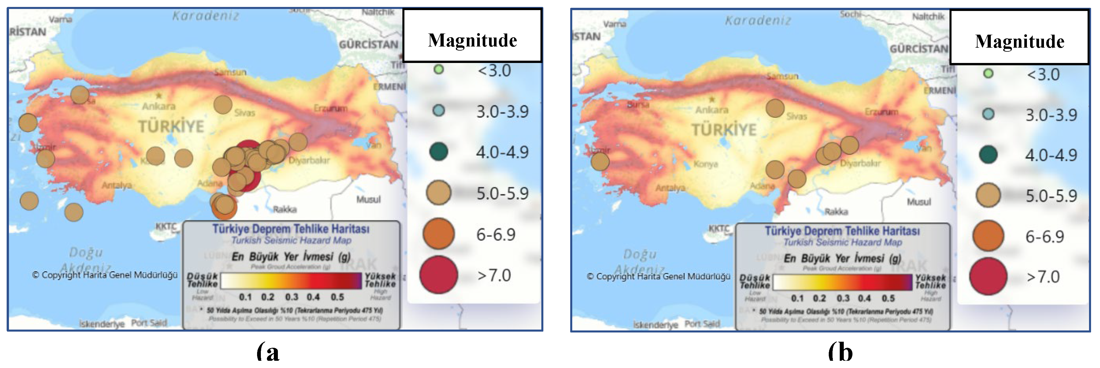
Figure 2.
Various views of the examined educational building: (a) Southeast facade; (b) Northeast facade; (c) east facade.
Figure 2.
Various views of the examined educational building: (a) Southeast facade; (b) Northeast facade; (c) east facade.
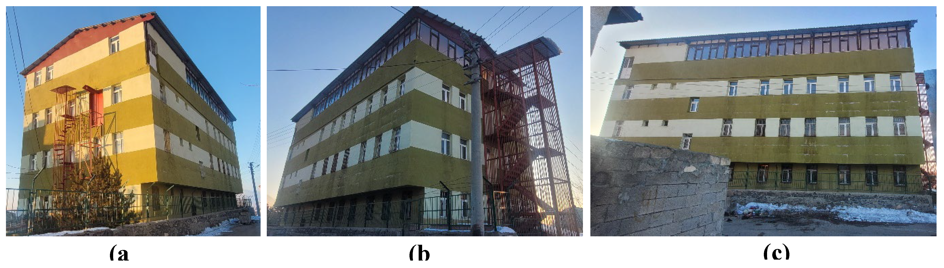
Figure 3.
Interior views of the examined building: (a) Second floor; (b) First floor.
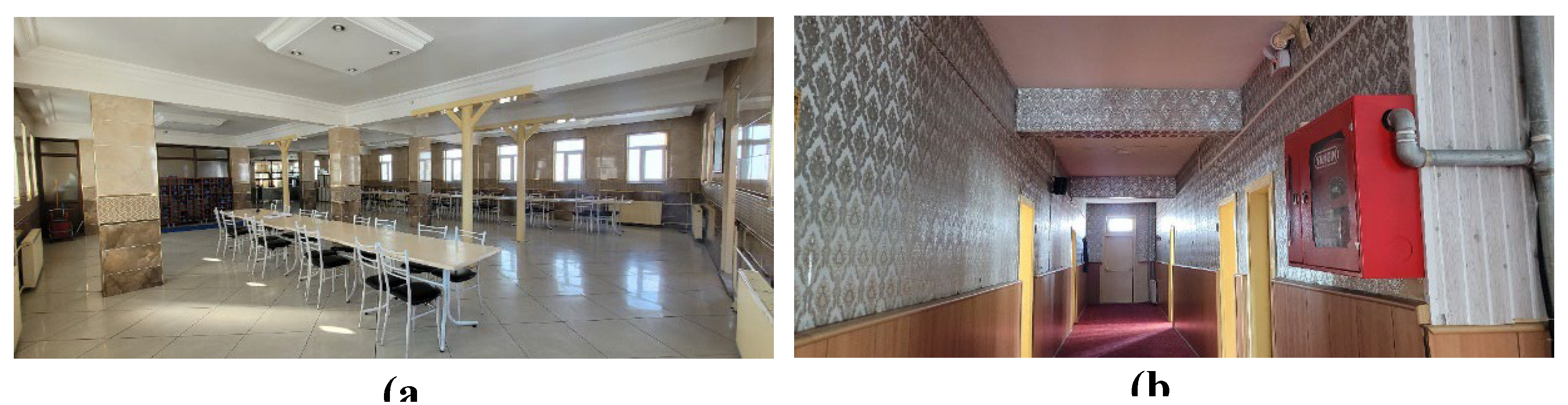
Figure 4.
Attic: (a) Meeting area; (b) Partition wall and roof support system.
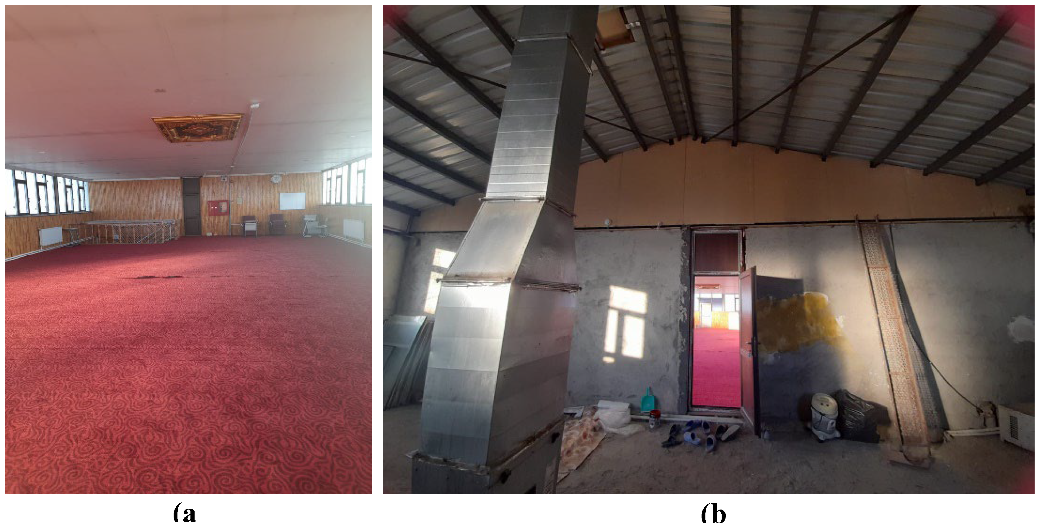
Figure 5.
Survey of the ground floor, second, and third floors.
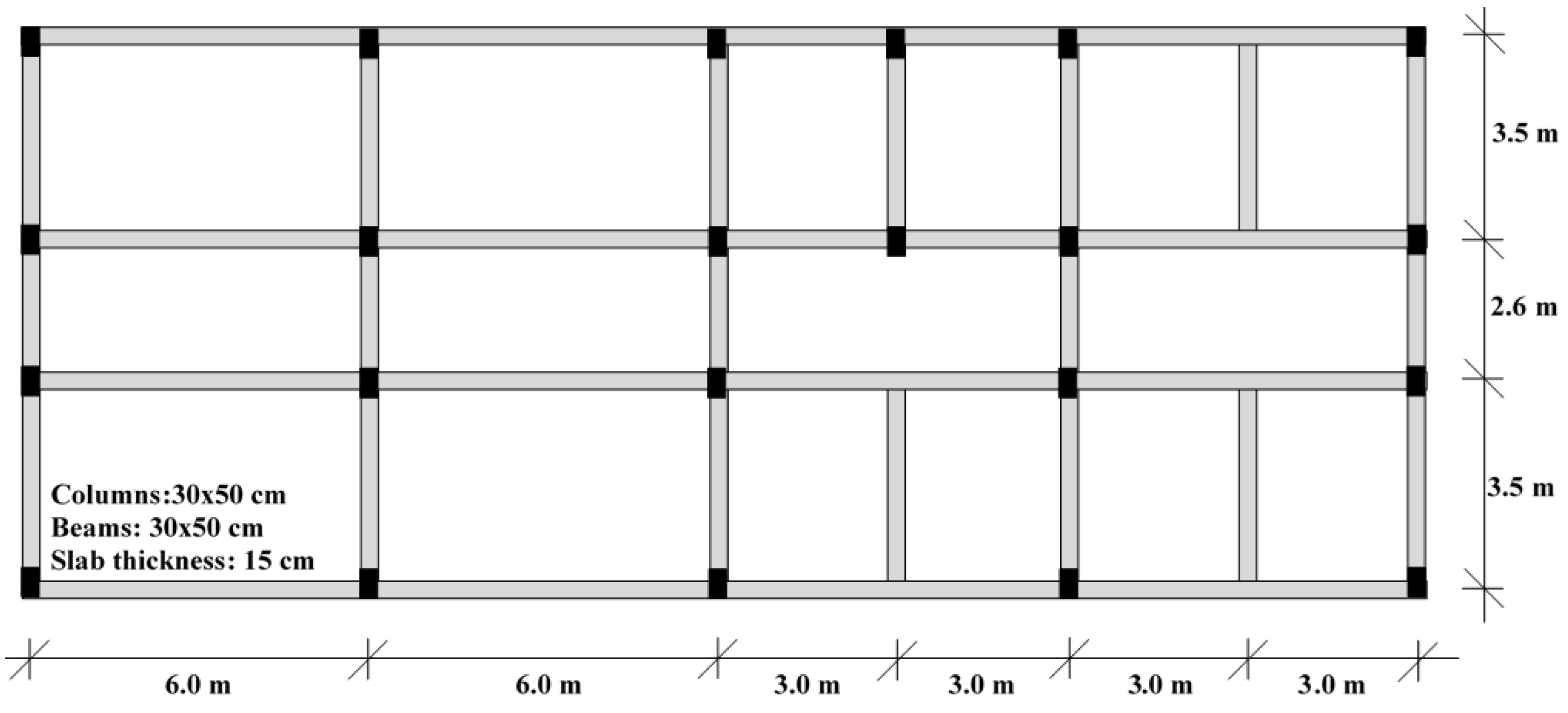
Figure 6.
Survey of the first floor.
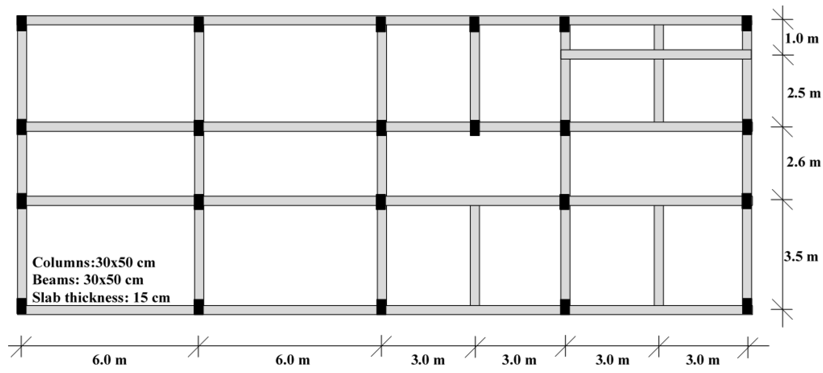
Figure 7.
Reinforced concrete sections determined as a result of the scanning application: (a) Column; (b) Beam.
Figure 7.
Reinforced concrete sections determined as a result of the scanning application: (a) Column; (b) Beam.
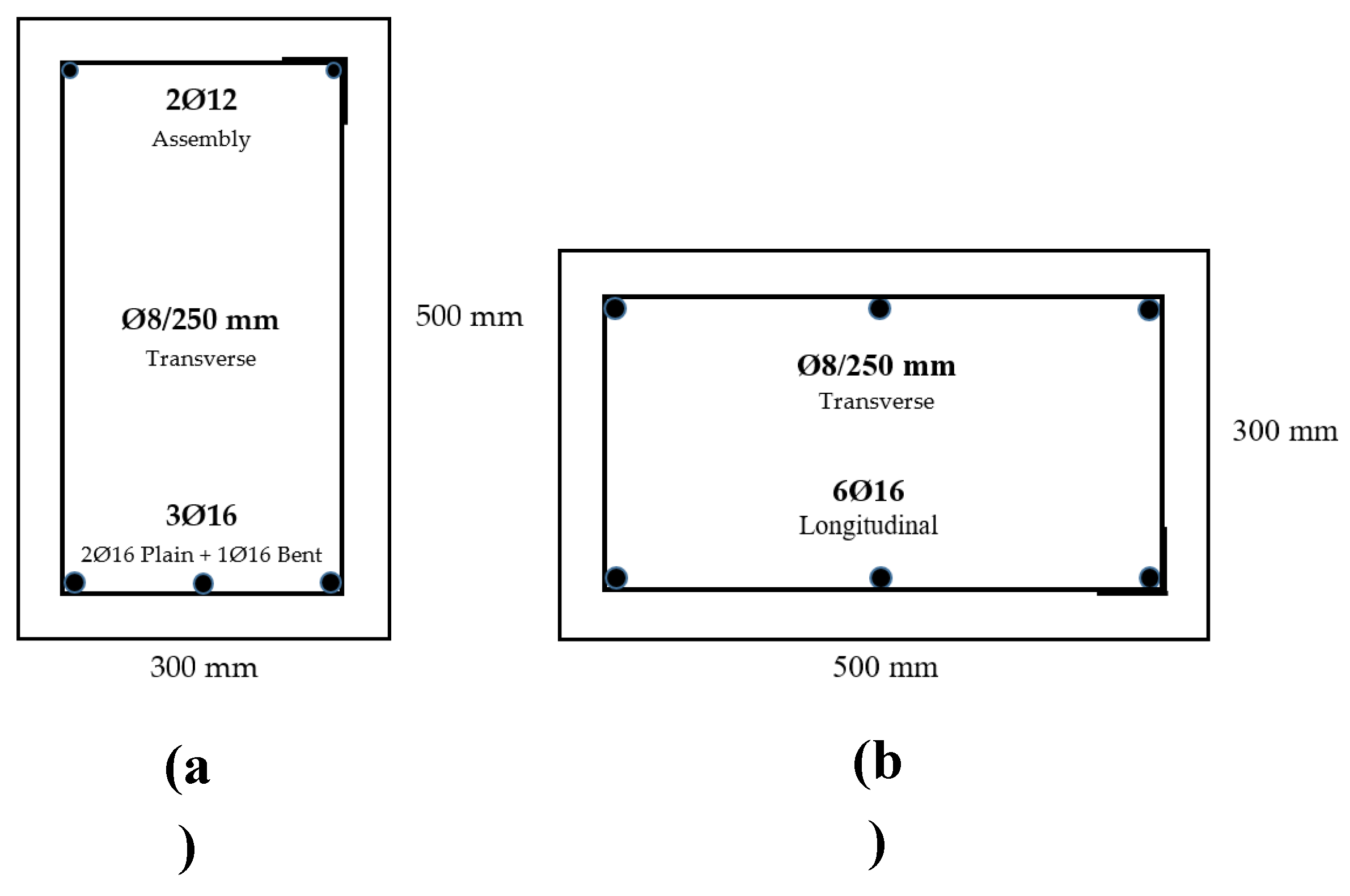
Figure 8.
Images from the reinforcement scanning process: (a) Beam; (b) Column.
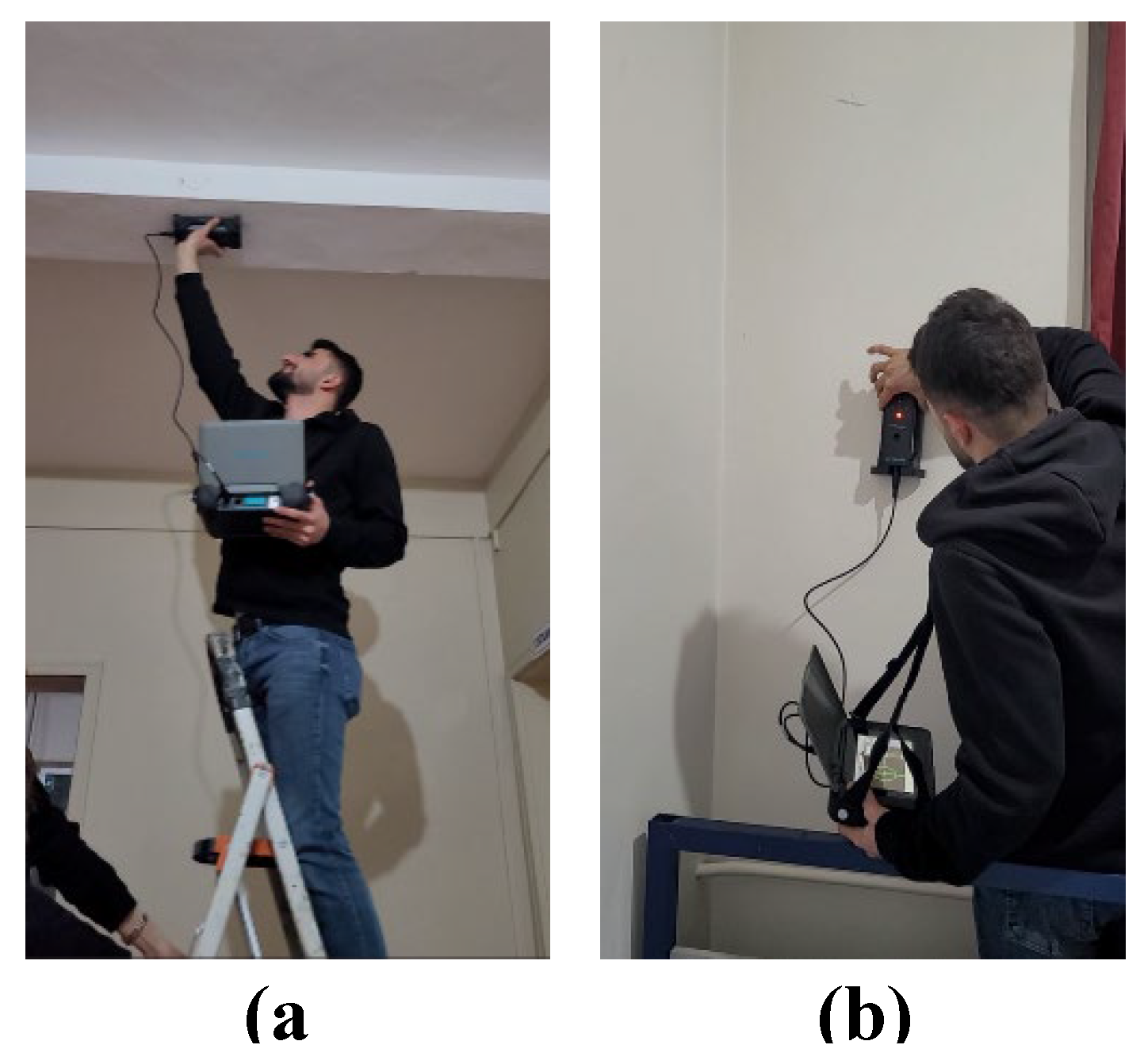
Figure 9.
Concrete sample taken from the column specimen.

Figure 10.
General view of the finite element model.
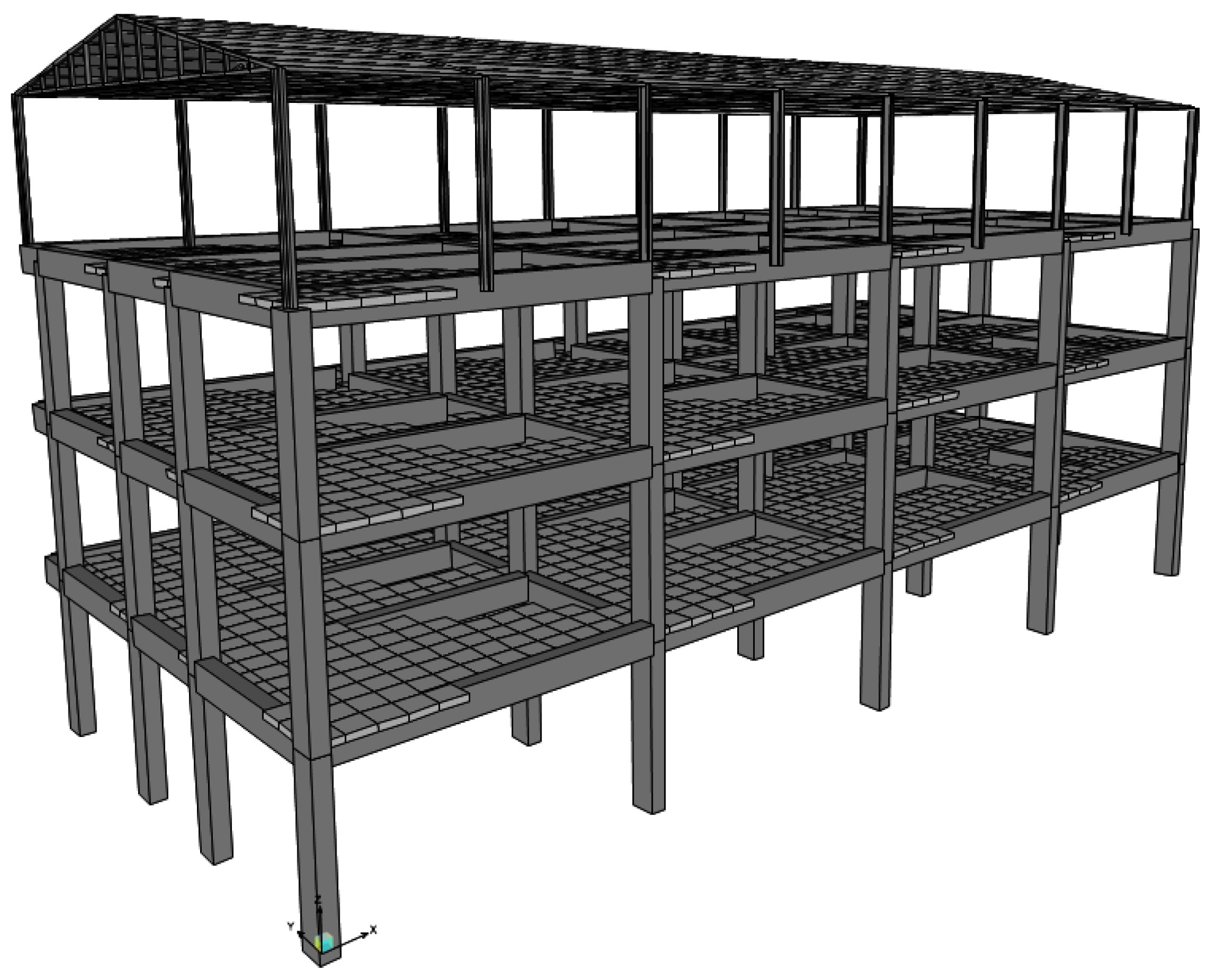
Figure 11.
Sensor layout plan for the OMA-1 application based on accelerometer placement.
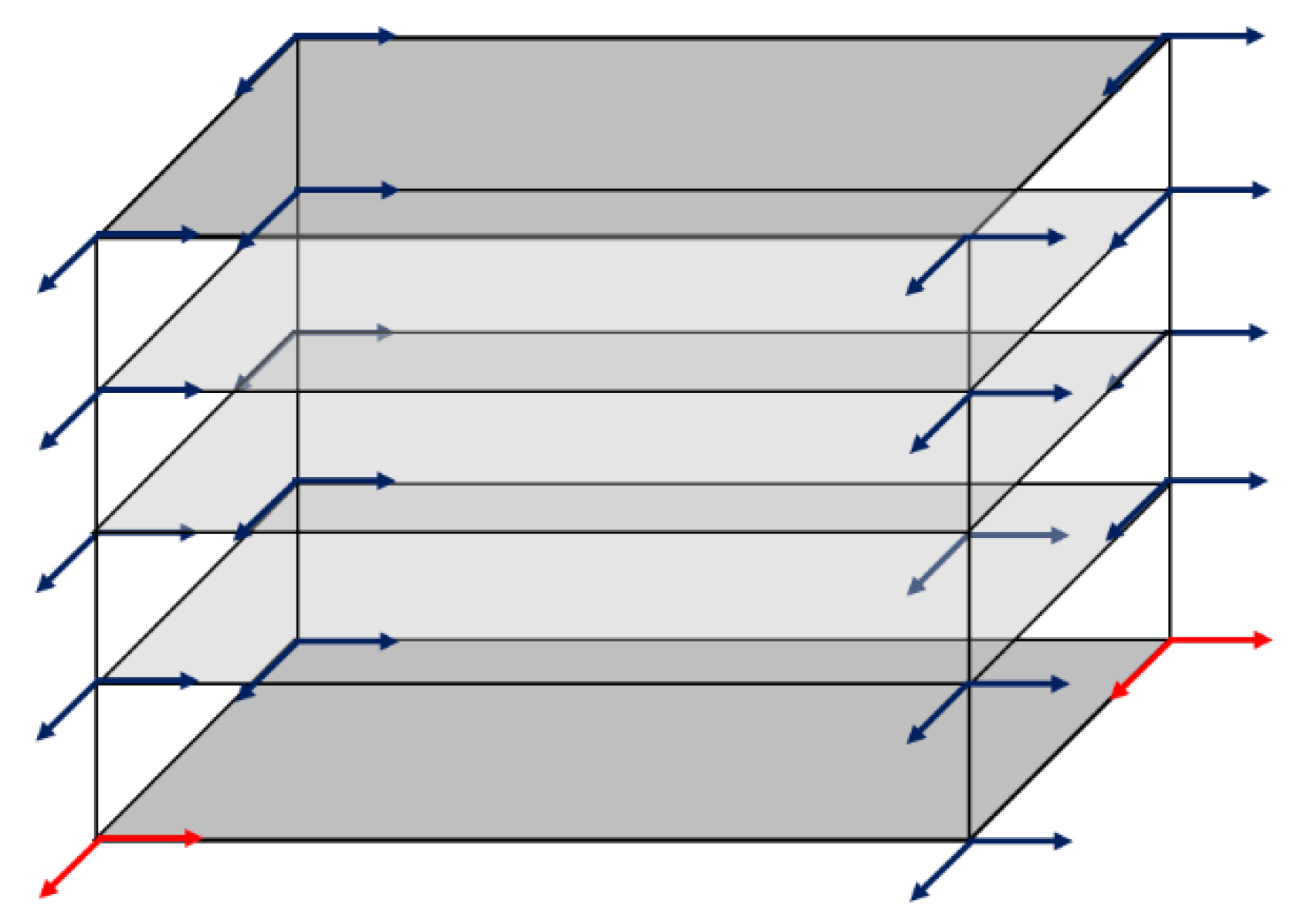
Figure 12.
Images from the response vibration measurement work within the scope of OMA applications: (a) Accelerometer sensors; (b) Data acquisition system.
Figure 12.
Images from the response vibration measurement work within the scope of OMA applications: (a) Accelerometer sensors; (b) Data acquisition system.
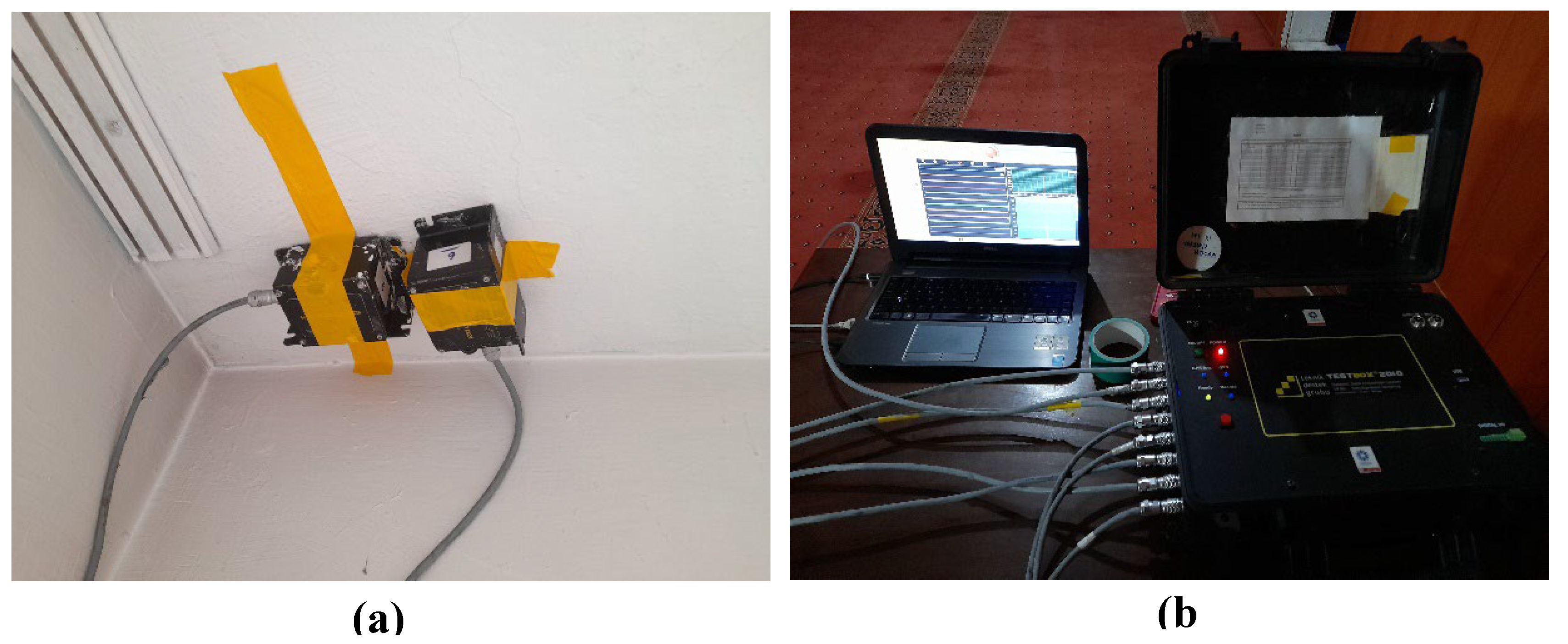
Figure 13.
Response vibration graphs recorded at a frequency of 100 Hz.
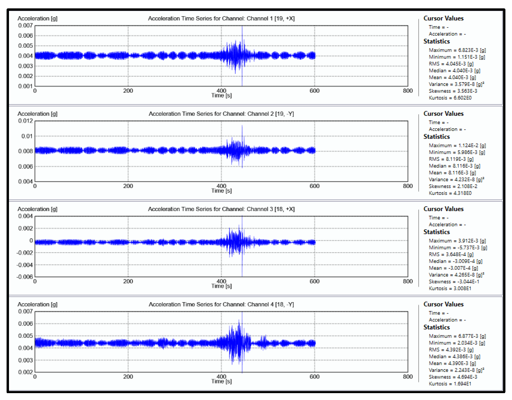
Figure 14.
The accelerometer sensor layout plan for the OMA-2 application.
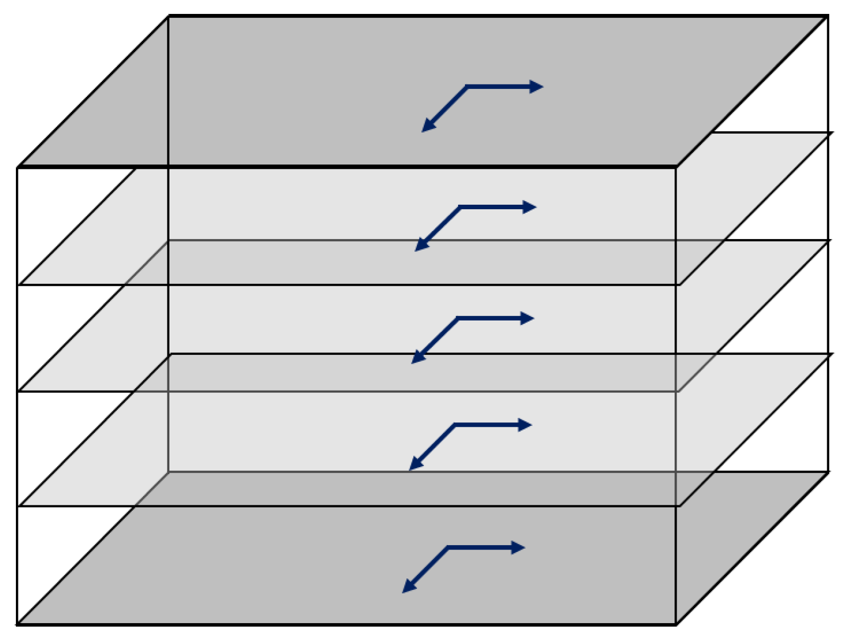
Figure 15.
Spectral density function graphs calculated for OMA-1 applications.
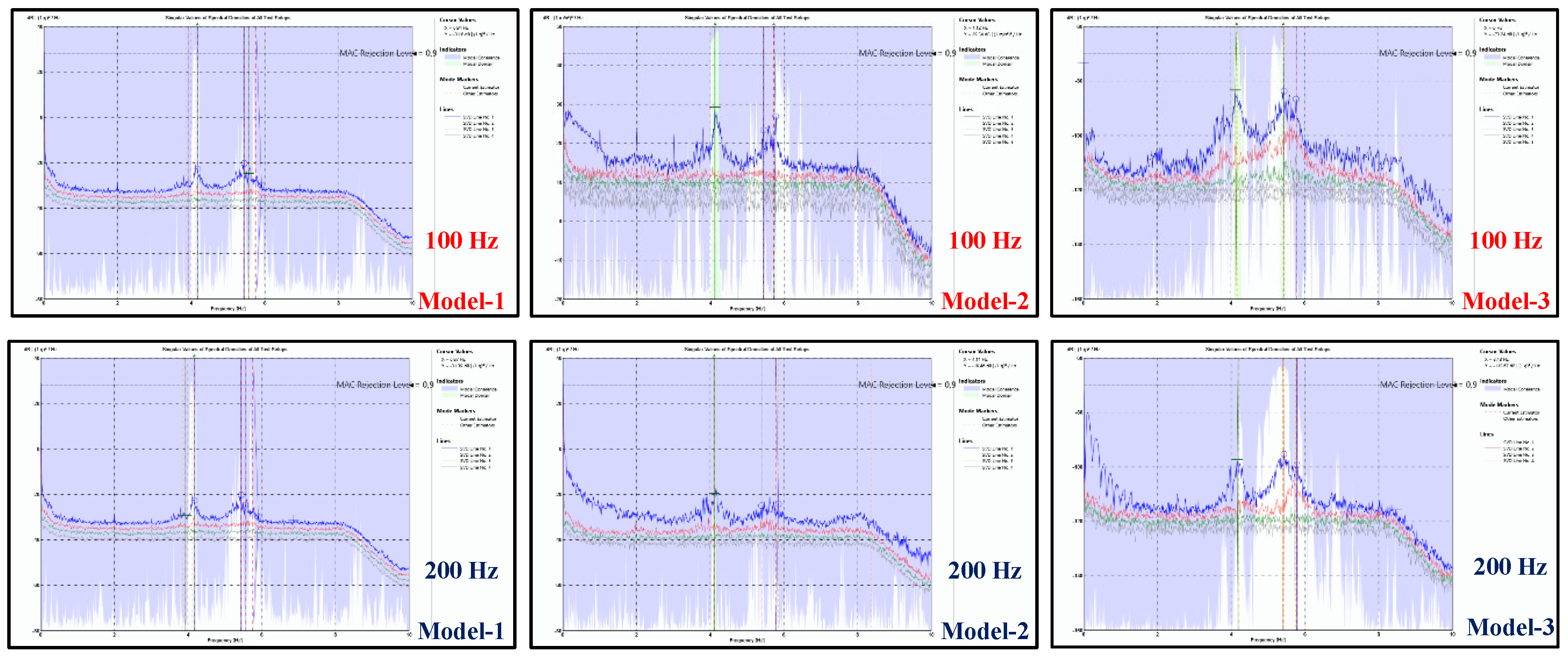
Figure 16.
The spectral density function graphs calculated for OMA-2 applications.
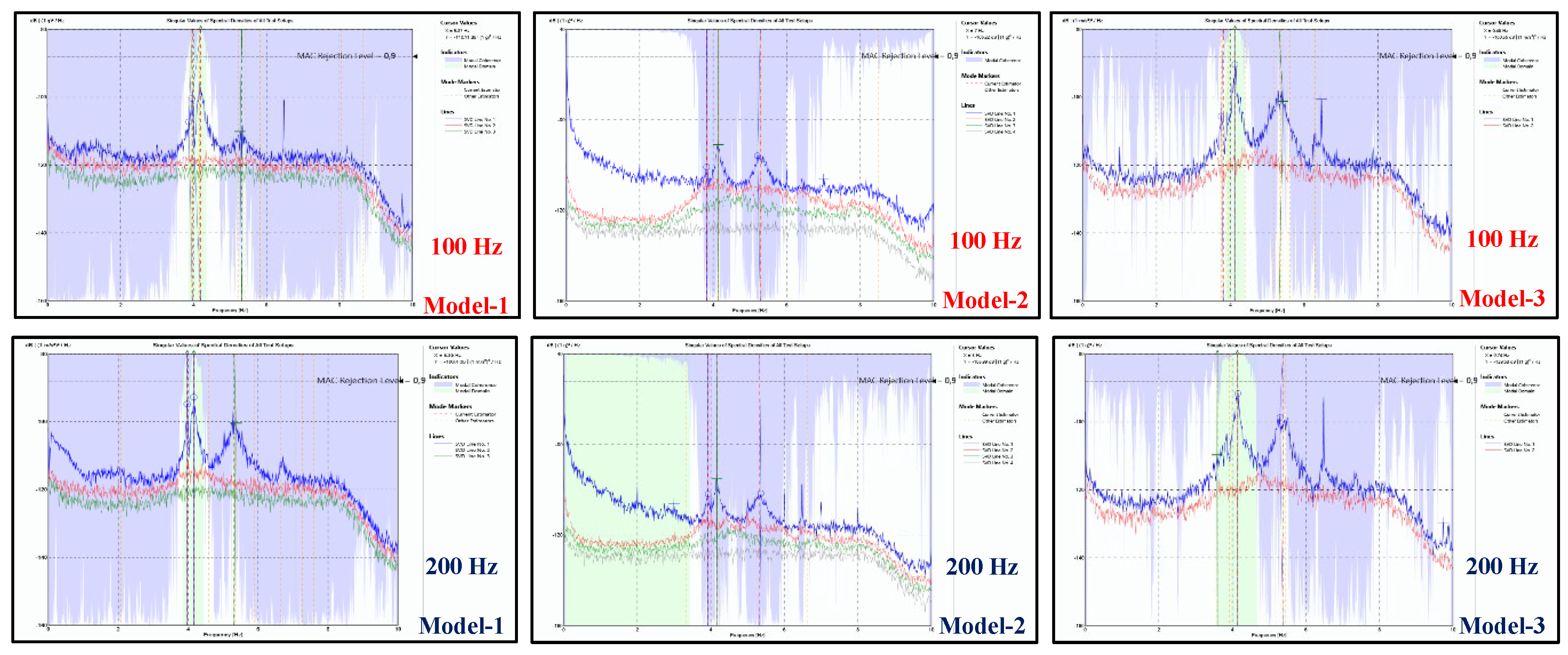
Figure 16.
Images of the Malatya Governor's Office after the February 6, 2023 Kahramanmaraş earthquakes: (a) Rear facade; (b) Side facade; (c) Interior of the building; (d) Damage to the column-beam connection inside the building.
Figure 16.
Images of the Malatya Governor's Office after the February 6, 2023 Kahramanmaraş earthquakes: (a) Rear facade; (b) Side facade; (c) Interior of the building; (d) Damage to the column-beam connection inside the building.
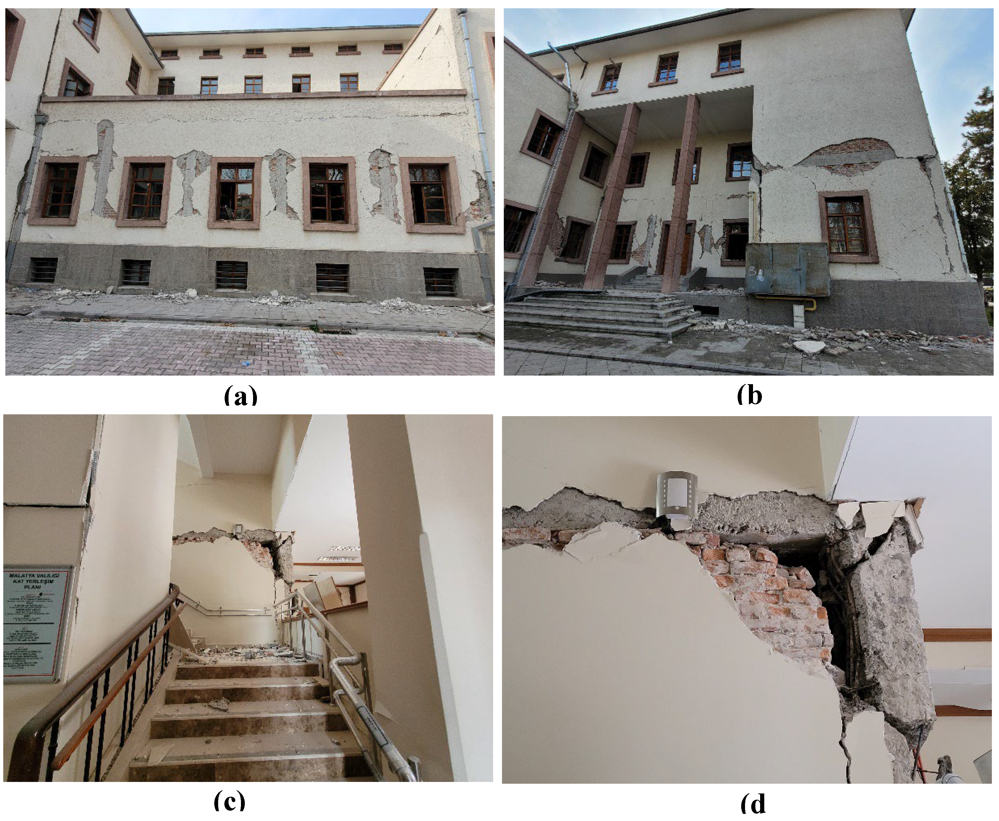
Figure 18.
Horizontal elastic design spectrum for the building studied.
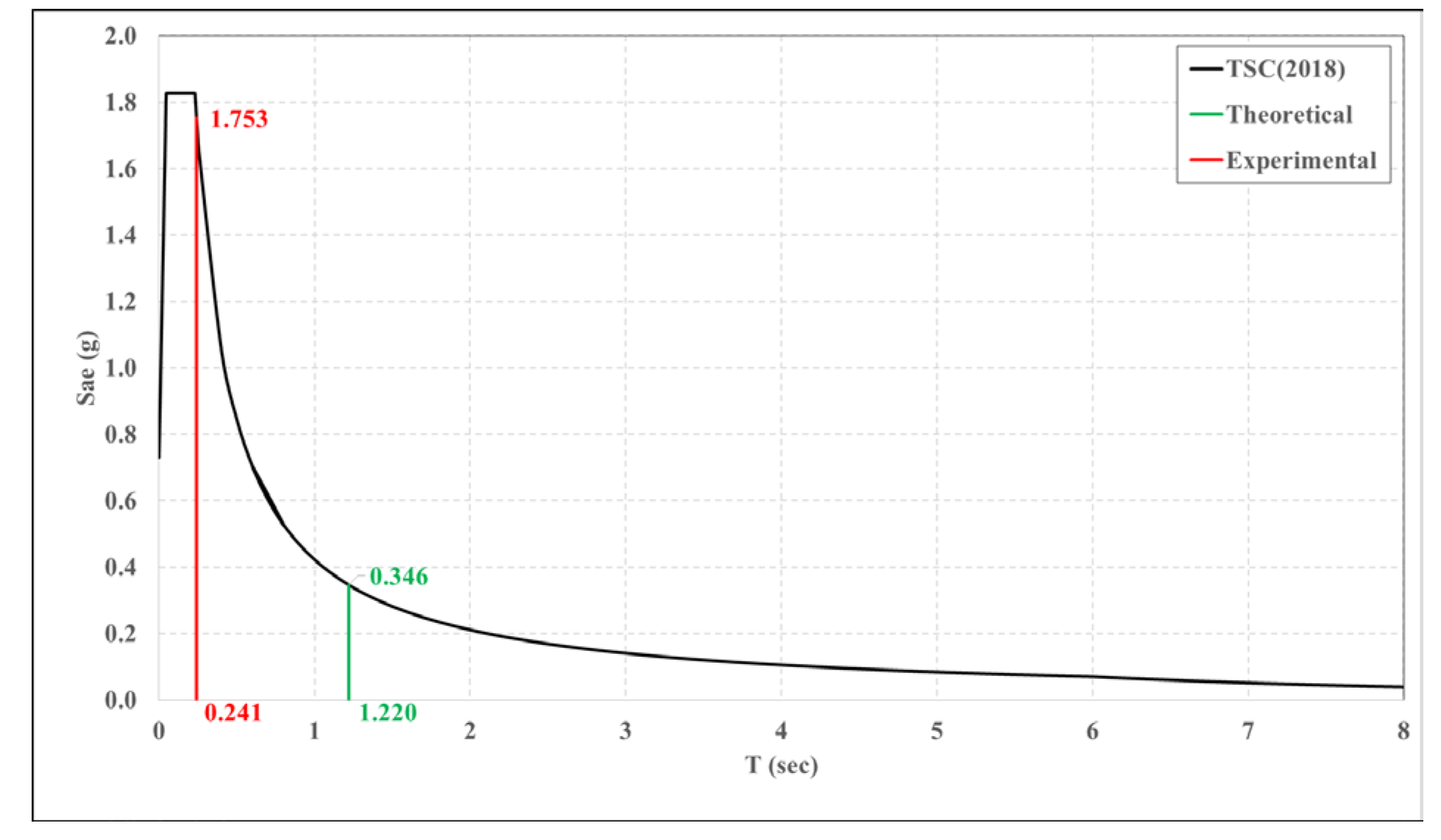

Table 1.
The top 10 countries with the highest earthquake risk according to the INFORM Risk 2025 report [6].
Table 1.
The top 10 countries with the highest earthquake risk according to the INFORM Risk 2025 report [6].
| Rank | Country | Earthquake Risk Score |
| 1 | Nepal | 9.8 |
| 2 | Philippines | 9.7 |
| 3 | Japan | 9.7 |
| 4 | Peru | 9.6 |
| 5 | Chilie | 9.6 |
| 6 | Ecuador | 9.5 |
| 7 | Guatemala | 9.5 |
| 8 | Iran | 9.3 |
| 9 | Türkiye | 9.3 |
| 10 | Pakistan | 9.2 |
Table 2.
Compressive strength test results of concrete samples.
| Specimen | Compressive Strength (MPa) |
| 1 | 11.7 |
| 2 | 8.2 |
| 3 | 8.4 |
| 4 | 12.8 |
| 5 | 12.7 |
| 6 | 11.6 |
| Mean: | 10.9 |
Table 3.
Theoretical natural vibration period calculation results for the examined building according to various codes.
Table 3.
Theoretical natural vibration period calculation results for the examined building according to various codes.
| Regulation/Code | Empirical Equation | Values of the Parameter | Period (s) |
| TSC(2007) [23] | TpA=Ct*HN3/4 | Ct=0.1, HN=13 m | 0.685 |
| TSC (2018) [19] | TpA=Ct*HN3/4 | Ct= 0.1, HN=13 m | 0.685 |
| ASCE 7-16 (2017) [24] | 0,1N | N=4 | 0.400 |
| ASCE 7-16 (2017) [24] | T= Ct*HNx | HN=13 m, Ct=0.0466, x=0.9 | 0.469 |
| Uniform Building Code(1997) [25] | T= Ct*HN3/4 | Ct : 0.0731, HN=13 m | 0.500 |
| Eurocode 8 (2004) [26] | T= Ct*H3/4 | Ct=0.075, HN=13 m | 0.513 |
| Iran Code (2007) [27] | T= 0.070*H3/4 | H=13 m | 0.479 |
| Israil Code (2009) [28] | T= 0.075*H3/4 | H=13 m | 0.513 |
| Indian Code (2002) [29] | T= 0.075*H3/4 | H=13 m | 0.513 |
Table 4.
Theoretical modal analysis results calculated on the finite element model.
| Mode Number | Mode Shape | Period (s) |
| 1 |
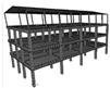 Horizontal translational movement parallel to the long plan direction |
1.220 |
| 2 |
 Horizontal translational movement parallel to short plan direction |
0.819 |
| 3 |
 Lateral torsional movement around the vertical axis |
0.800 |
| 4 |
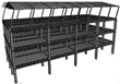 Horizontal translational movement of the roof floor parallel to the long plan direction* |
0.793 |
| 5 |
 Vertical torsional movement around the short span direction of the structure |
0.392 |
* Mode shapes related to the local movement of roof floor itself is explained by italic fonts in this table and beyond.
Table 5.
Modal behavior characteristics obtained from OMA-1 application (100 Hz).
| Model-1 | Model-2 | Model-3 | ||||
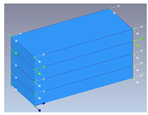 Sensor placement in all floors |
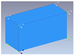 Sensor placement in the ground floor and the top floor |
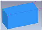 Sensor placement in only the top floor |
||||
| Mode Number | Mode Shape | Period (s) | Mode Shape | Period (s) | Mode Shape | Period (s) |
| 1 | Horizontal translational movement of the roof floor parallel to the short plan direction | 0.254 | Horizontal translational movement parallel to the short plan direction | 0.243 | Horizontal translational movement parallel to the short plan direction | 0.241 |
| 2 | Horizontal translational movement parallel to the short plan direction | 0.240 | Horizontal translational movement parallel long plan direction | 0.184 | Horizontal translational movement parallel long plan direction | 0.184 |
| 3 | Horizontal translational movement parallel long plan direction | 0.184 | Lateral torsional movement around the vertical axis | 0.175 | Lateral torsional movement around the vertical axis | 0.173 |
| 4 | Lateral torsional movement of the roof floor around the vertical axis | 0.180 | - | - | - | - |
| 5 | Lateral torsional movement around the vertical axis | 0.174 | - | - | - | - |
Table 6.
Modal behavior characteristics obtained from OMA-1 application (200 Hz).
| Model-1 | Model-2 | Model-3 | ||||
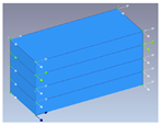 Sensor placement in all floors |
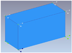 Sensor placement in the ground floor and the top floor |
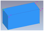 Sensor placement in only the top floor |
||||
| Mode Number | Mode Shape | Period (s) | Mode Shape | Period (s) | Mode Shape | Period (s) |
| 1 | Horizontal translational movement of the roof floor parallel to the short plan direction | 0.257 | Horizontal translational movement parallel to the short plan direction | 0.243 | Horizontal translational movement parallel to the short plan direction | 0.239 |
| 2 | Horizontal translational movement parallel to the short plan direction | 0.243 | Horizontal translational movement parallel long plan direction | 0.185 | Horizontal translational movement parallel long plan direction | 0.185 |
| 3 | Horizontal translational movement parallel long plan direction | 0.183 | Lateral torsional movement around the vertical axis | 0.173 | Lateral torsional movement around the vertical axis | 0.173 |
| 4 | Lateral torsional movement of the roof floor around the vertical axis | 0.178 | - | - | - | - |
| 5 | Lateral torsional movement around the vertical axis | 0.173 | - | - | - | - |
Table 7.
Modal behavior characteristics obtained from OMA-1 application (mean).
| Model-1 | Model-2 | Model-3 | ||||
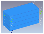 Sensor placement in all floors |
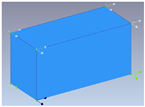 Sensor placement in the ground floor and the top floor |
 Sensor placement in only the top floor |
||||
| Mode Number | Mode Shape | Period (s) | Mode Shape | Mode Number | Mode Shape | Period (s) |
| 1 | Horizontal translational movement of the roof floor parallel to the short plan direction | 0.255 | Horizontal translational movement parallel to the short plan direction | 0.243 | Horizontal translational movement parallel to the short plan direction | 0.240 |
| 2 | Horizontal translational movement parallel to the short plan direction | 0.242 | Horizontal translational movement parallel long plan direction | 0.185 | Horizontal translational movement parallel long plan direction | 0.185 |
| 3 | Horizontal translational movement parallel long plan direction | 0.183 | Lateral torsional movement around the vertical axis | 0.174 | Lateral torsional movement around the vertical axis | 0.173 |
| 4 | Lateral torsional movement of the roof floor around the vertical axis | 0.179 | - | - | - | - |
| 5 | Lateral torsional movement around the vertical axis | 0.173 | - | - | - | - |
Table 8.
Final Mode Shapes and Period Values Obtained from the OMA-1 Application.
| Mode Number | Mode Shape | Period (s) |
| 1 | Horizontal translational movement of the roof floor parallel to the short plan direction | 0.255 |
| 2 | Horizontal translational movement parallel to the short plan direction | 0.241 |
| 3 | Horizontal translational movement parallel long plan direction | 0.184 |
| 4 | Lateral torsional movement of the roof floor around the vertical axis | 0.179 |
| 5 | Lateral torsional movement around the vertical axis | 0.173 |
Table 9.
MAC values calculated for OMA-1 applications.
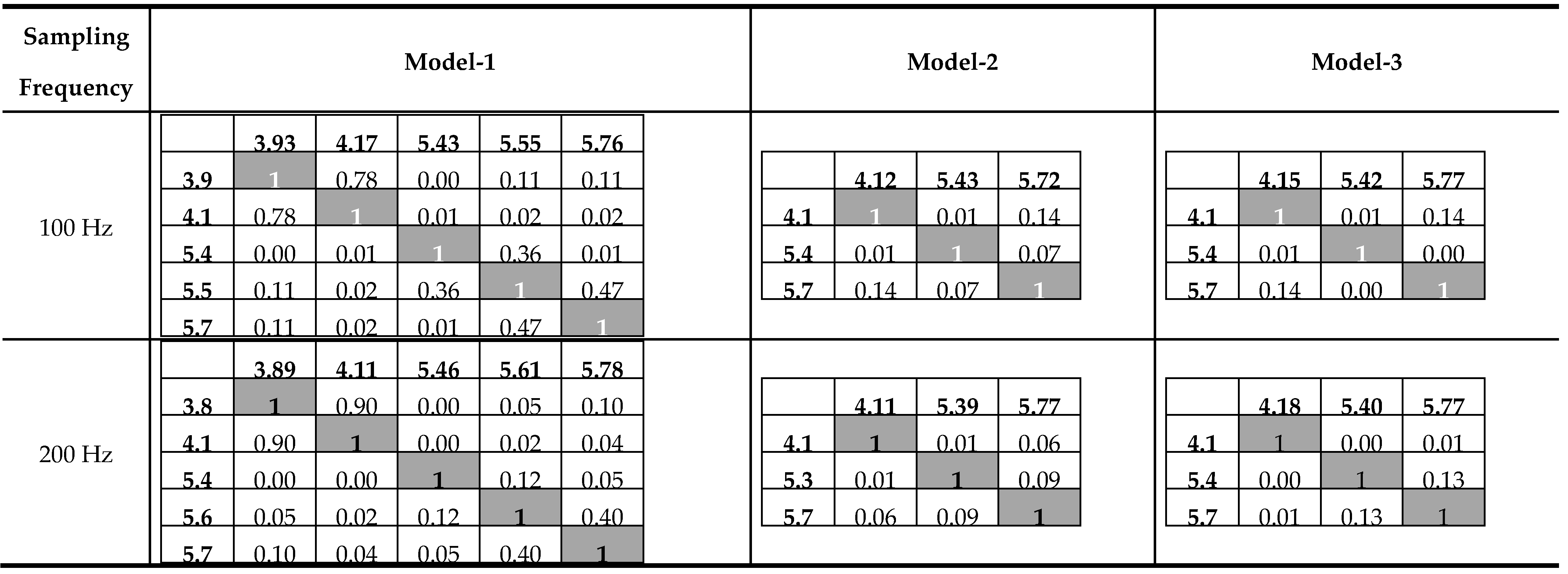
Table 10.
Modal Behavior Characteristics Obtained from the OMA-2 Application (100 Hz).
| Model-1 | Model-2 | Model-3 | ||||
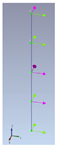 Sensor placement in all floors |
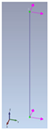 Sensor placement in the ground floor and the top floor |
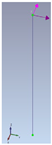 Sensor placement in only the top floor |
||||
| Mode Number | Mode Shape | Period (s) | Mode Shape | Period (s) | Mode Shape | Period (s) |
| 1 | Horizontal translational movement parallel to the short plan direction | 0.252 | Horizontal translational movement parallel to the short plan direction | 0.261 | Horizontal translational movement parallel to the short plan direction | 0.263 |
| 2 | Horizontal translational movement parallel to the short plan direction | 0.238 | Horizontal translational movement parallel to the short plan direction | 0.242 | Horizontal translational movement parallel to the short plan direction | 0.242 |
| 3 | Horizontal translational movement parallel long plan direction | 0.188 | Horizontal translational movement parallel long plan direction | 0.189 | Horizontal translational movement parallel long plan direction | 0.188 |
Table 11.
Modal Behavior Characteristics Obtained from the OMA-2 Application (200 Hz).
| Model-1 | Model-2 | Model-3 | ||||
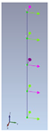 Sensor placement in all floors |
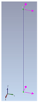 Sensor placement in the ground floor and the top floor |
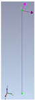 Sensor placement in only the top floor |
||||
| Mode Number | Mode Shape | Period (s) | Mode Shape | Period (s) | Mode Shape | Period (s) |
| 1 | Horizontal translational movement parallel to the short plan direction | 0.252 | Horizontal translational movement parallel to the short plan direction | 0.255 | Horizontal translational movement parallel to the short plan direction | 0.278 |
| 2 | Horizontal translational movement parallel to the short plan direction | 0.240 | Horizontal translational movement parallel to the short plan direction | 0.240 | Horizontal translational movement parallel to the short plan direction | 0.242 |
| 3 | Horizontal translational movement parallel long plan direction | 0.188 | Horizontal translational movement parallel long plan direction | 0.188 | Horizontal translational movement parallel long plan direction | 0.186 |
Table 12.
Modal Behavior Characteristics Obtained from the OMA-2 Application (Average).
| Model-1 | Model-2 | Model-3 | ||||
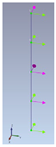 Sensor placement in all floors |
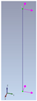 Sensor placement in the ground floor and the top floor |
 Sensor placement in only the top floor |
||||
| Mode Number | Mode Shape | Period (s) | Mode Shape | Period (s) | Mode Shape | Period (s) |
| 1 | Horizontal translational movement parallel to the short plan direction | 0.252 | Horizontal translational movement parallel to the short plan direction | 0.258 | Horizontal translational movement parallel to the short plan direction | 0.270 |
| 2 | Horizontal translational movement parallel to the short plan direction | 0.239 | Horizontal translational movement parallel to the short plan direction | 0.241 | Horizontal translational movement parallel to the short plan direction | 0.242 |
| 3 | Horizontal translational movement parallel long plan direction | 0.188 | Horizontal translational movement parallel long plan direction | 0.188 | Horizontal translational movement parallel long plan direction | 0.187 |
Table 13.
The final modal behavior characteristics obtained as a result of the OMA-2 application.
| Mode Number | Mode Shape | Period (s) |
| 1 | Horizontal translational movement parallel to the short plan direction | 0.260 |
| 2 | Horizontal translational movement parallel to the short plan direction | 0.241 |
| 3 | Horizontal translational movement parallel long plan direction | 0.188 |
Table 14.
MAC values calculated for OMA-2 applications.
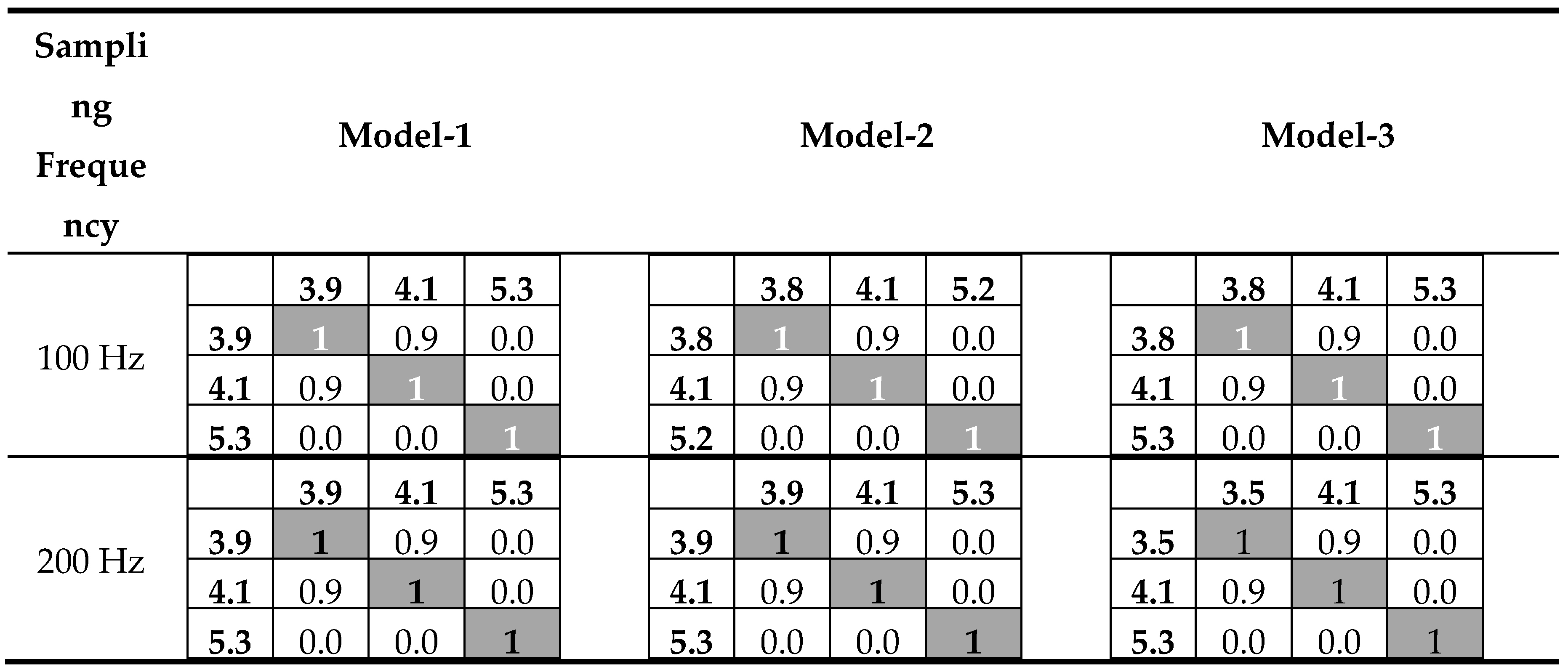
Table 15.
Results of theoretical and experimental modal analysis.
| Theoretical Modal Anlysis | Operational Modal Analysis | |||||
| RYTEİE (2019) | OMA-1 | OMA-2 | ||||
| Mode Number | Mode Shape | Period (s) | Mode Shape | Period (s) | Mode Shape | Period (s) |
| 1 | Horizontal translational movement parallel to the long plan direction | 1.220 | Horizontal translational movement of the roof floor parallel to the short plan direction | 0.255 | Horizontal translational movement parallel to the short plan direction | 0.260 |
| 2 | Horizontal translational movement parallel to the short plan direction | 0.819 | Horizontal translational movement parallel to the short plan direction | 0.241 | Horizontal translational movement parallel to the short plan direction | 0.241 |
| 3 | Lateral torsional movement around the vertical axis |
0.800 | Horizontal translational movement parallel long plan direction | 0.184 | Horizontal translational movement parallel long plan direction | 0.188 |
| 4 | Horizontal translational movement of the roof floor parallel to the long plan direction | 0.793 | Lateral torsional movement of the roof floor around the vertical axis | 0.179 | - |
- |
| 5 | Vertical torsional movement around the short span direction of the structure | 0.392 | Lateral torsional movement around the vertical axis | 0.173 | - | - |
Table 16.
Calculations of the natural vibration period for the examined building's structural system, considering the presence of shear walls, according to various regulations.
Table 16.
Calculations of the natural vibration period for the examined building's structural system, considering the presence of shear walls, according to various regulations.
| Regulation/Code | Empirical Equation | Value of the Parameter | Period (s) |
| TSC(1998) [63] | T=Ct*HN3/4 | Ct=0.05, HN=13 m | 0.342 |
| TSC(2007) [23] | TpA=Ct*HN3/4 | Ct=0.07, HN=13 m | 0.479 |
| TSC (2018) [19] | TpA=Ct*HN3/4 | Ct= 0.07, HN=13 m | 0.479 |
| ASCE 7-16 (2017) [24] | 0,1N | N=4 | 0.400 |
| ASCE 7-16 (2017) [24] | T= Ct*HNx | HN=13 m, Ct=0.0488, x=0.75 | 0.334 |
| Uniform Building Code(1997) [25] | T= Ct*HN3/4 | Ct : 0.0488, HN=13 m | 0.334 |
| Eurocode 8 (2004) [26] | T= Ct*H3/4 | Ct=0.05, HN=13 m | 0.342 |
| Iran Code (2007) [27] | T= 0.050*H3/4 | H=13 m | 0.342 |
| Israil Code (2009) [28] | T= 0.050*H3/4 | H=13 m | 0.342 |
Table 17.
Relations proposed for calculating the natural vibration period in studies [69,70,71,72,73] and the period values calculated for the examined structure.
| Study | Empirical Equation | Period (s) |
| Chopra and Goel (2000) [69] | T= 0.067*H0.9 | 0.674 |
| Hong and Hwang (2000) [70] | T= 0.0294*H0.804 | 0.231 |
| Crowley and Pinho (2006) [71] | T= 0.055*H | 0.715 |
| Güler et al. (2008)[72] | T= 0.026*H0.9 | 0.262 |
| Hatzigeorgiou and Kanapitsas (2013) [73] | T= 0.075*H0.75 | 0.452 |
Disclaimer/Publisher’s Note: The statements, opinions and data contained in all publications are solely those of the individual author(s) and contributor(s) and not of MDPI and/or the editor(s). MDPI and/or the editor(s) disclaim responsibility for any injury to people or property resulting from any ideas, methods, instructions or products referred to in the content. |
© 2025 by the authors. Licensee MDPI, Basel, Switzerland. This article is an open access article distributed under the terms and conditions of the Creative Commons Attribution (CC BY) license (http://creativecommons.org/licenses/by/4.0/).
Copyright: This open access article is published under a Creative Commons CC BY 4.0 license, which permit the free download, distribution, and reuse, provided that the author and preprint are cited in any reuse.


