1. Introduction
Higher dimensional - quantum optical communications is a subject of very significant current interest [
1,
2,
3]. It enables the transfer of higher dimensional quantum states using structured light, enabling more resilient quantum protocols and the investigation of new quantum phenomena such as hyper – entanglement. Methods for generating hyper-entangled states of light are found in [
2]. Mode coupling among photons traveling in different quantum channels during transmission however causes interference among signals and limits detection. Principal mode transmission [
4,
5,
6] is a means to deal with this limitation and can be implemented with quantum technologies.
A principal mode is a superposition of the N guided modes in a multimode fiber or few - mode fiber [
5]. If N guided modes exist within the fiber there exist N principal modes and the principal modes are a specific superposition of the fiber’s guided modes. The principal modes are orthogonal to each other and therefore cross talk free transmission can occur using these superpositions. They are independent of frequency to first order and this fact can be used to determine these modes [
5].
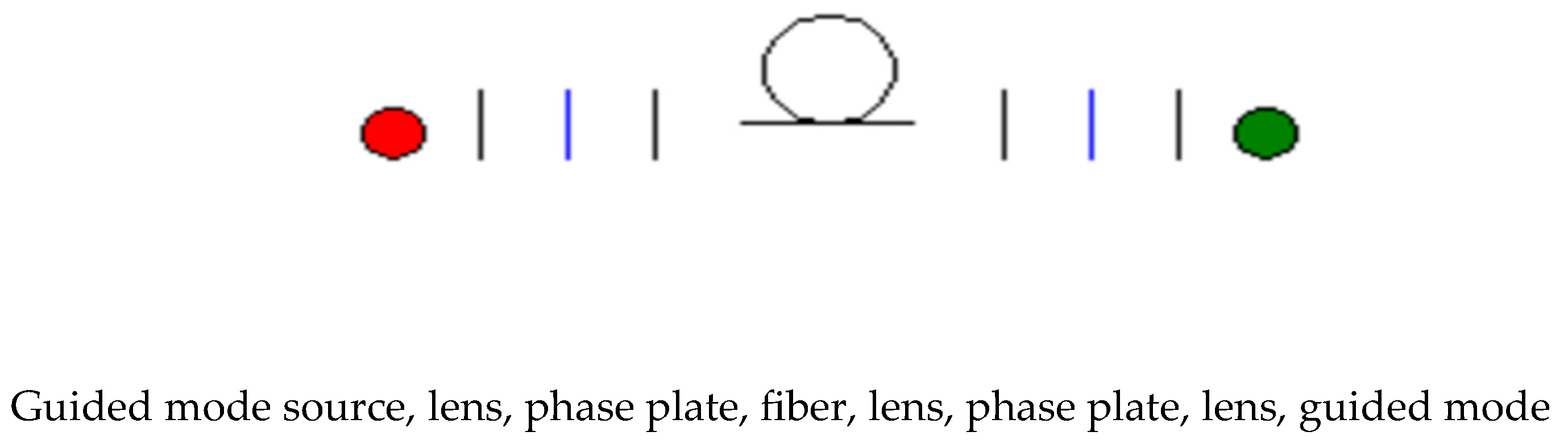
Figure 1 is a simplified schematic showing the component figuration required to implement principal state transmission. A source suitable for implementing guided transmission in the fiber is first passed through a lens and a spatial modulator, in order to implement the required phase transitions enabling the superpositions of modes. The light is then focused onto the fiber. At the output of the fiber, the superimposed modes are converted back to a specific guided mode or onto a detector. The guided mode can be hyperentangled. For example, it can contain a specific polarization state and a specific spatial mode. It can then be stored in an appropriate memory, for entanglement swapping. Determining these modes is a subject of significant interest and is the subject of section II.
In single mode fiber, there exist two orthogonal polarization states. These two states are not necessarily principal modes, so cross talk can occur when they are used to multiplex signals. However, principal polarization modes can be determined, and they used to send information over two separate channels [
5] without interference. In many quantum - communication protocols a polarization state in single mode fiber is used to communicate; and in quantum systems using entanglement swapping relating the polarization state at the output to input is necessary [
7]. Ulrich and Simon theoretically investigated this polarization state evolution in single mode fiber. This understanding is critical for tracking the polarization state and its evolution during transmission in quantum communication protocols. Ulrich and Simon [
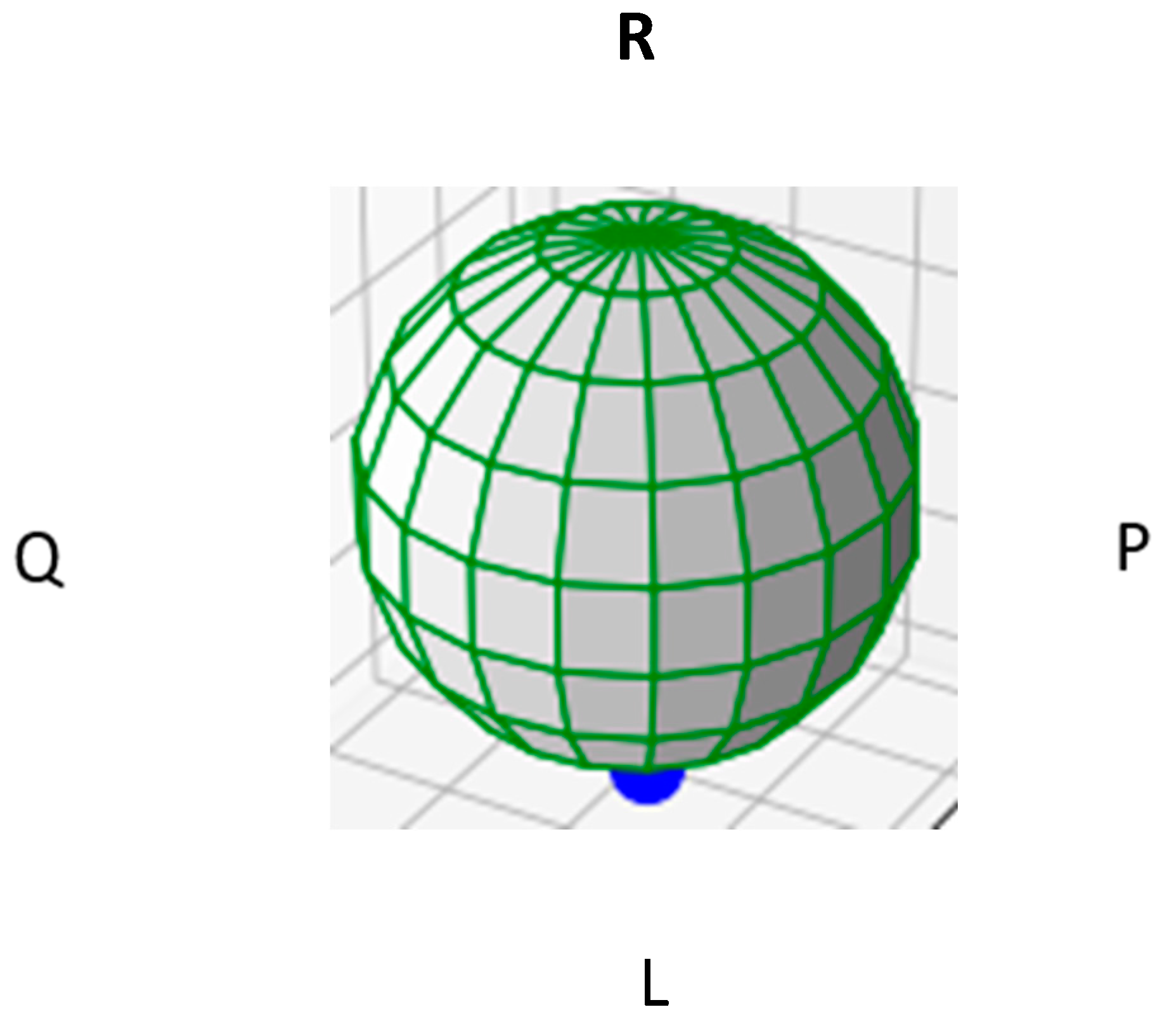
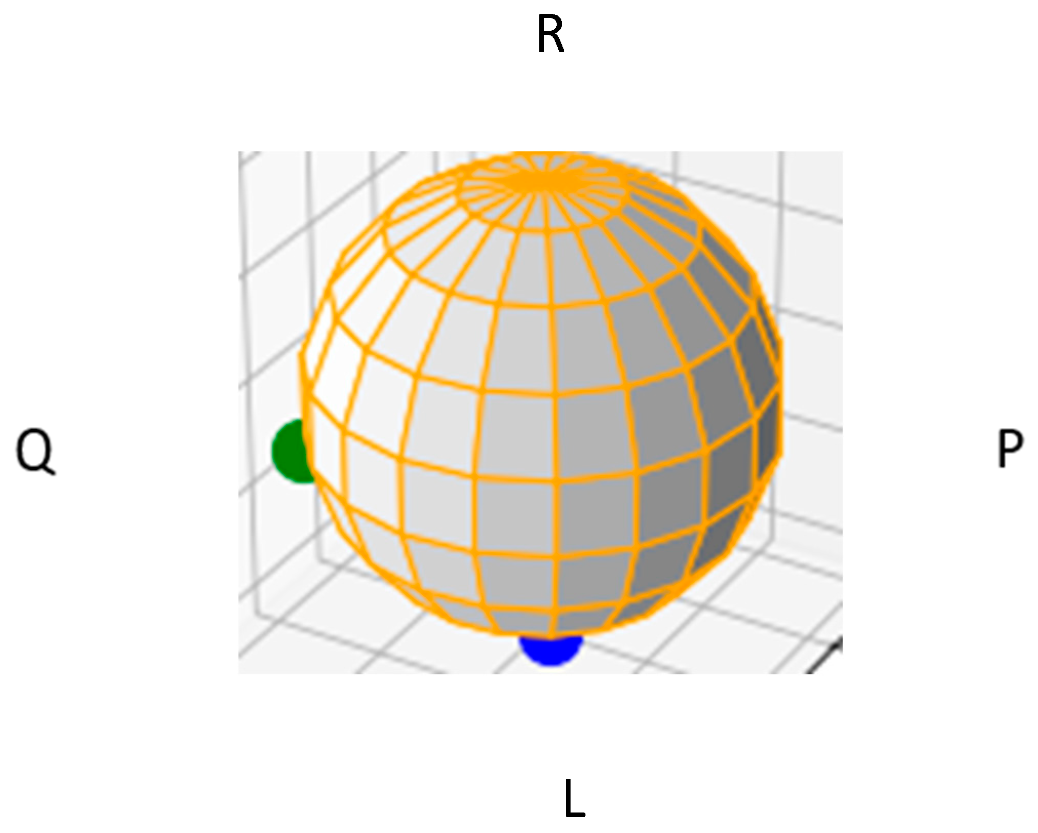
8] used the Poincare sphere to quantify this evolution. The polarization state in an optical fiber can be linearly, circularly or elliptically polarized and this state can evolve as the pulse travels in time. The Poincare sphere enables us to display these states and it is particularly important in relating the input polarization state to that at the output. On the sphere, P and Q represent positions of linear polarization, X and Y; while L and R represents points of circular polarization, left and right. In quantum communication systems, the output polarization is first set to be similar to the input state using classical communications and polarization controllers, which are well known commercial devices. The output polarization state can drift in time, on the order of seconds, so corrections are required. As an example,
Figure 2 shows the Poincare sphere with the polarization displayed in a linear state. The notation
In multimode fiber, and in the weak guidance approximation, each higher order – spatial mode contains two polarization states. These spatial modes can be characterized using the well-known linearly polarized modal numbers, LPnm [
9]. Here n quantifies the radial modal and m quantifies the azimuthal number, and also quantifies the orbital angular momentum. Similar to the Poincare sphere, Milione, Sztul, Nolan and Alfano [
10] introduced a higher order Poincare sphere (HOPS) to display these states.
For a specific - spatial LPnm mode, this state can be in an OAM, orbital angular momentum state or it can be in a a combination of OAM states. For this reason, it could be in the linear or elliptical rather than circular state. For this reason, displaying this mode on the higher order sphere is very useful. Because spatial modes contain two polarizations, we propose a combined polarization – spatial sphere displaying both spatial and polarization states,
Figure 4.
In higher order quantum communications, using spatial modes it is important to recover not only the original polarization state, but also the original spatial state. This can be achieved using polarization controllers for the polarization recovery and spatial light modulators to recover the spatial mode. In fact, spatial light modulators can be used to recover both the polarization and the spatial states. This will be discussed further below. Since the principal modes are orthogonal, one can use them for multiplexing.
2. Principal Modes
Principal modes for multiplexing multimode channels in optical fibers was first proposed by Kahn [
4,
5]. Carpenter [
11] was the first to measure these modes using a few mode fiber, polarization controllers, and spatial light modulators. Using a configuration like the simplified schematic in figure 1, he measured a mode transfer matrix, and from this matrix found an approximation to the principal modes of the fiber. The approximation is valid for weak mode coupling within the fiber. Xiong et. al. [
12] used a similar experimental configuration and the modal transfer matrix and then determined the principal modes in the case of strong coupling. Using transfer matrices at different wavelengths, they mathematically determined a group delay matrix and subsequently found a principal mode independent of frequency to first order. They showed the group delay matrix coincides with the Wigner – Smith time delay matrix, which is important in the study of the fundamentals of electromagnetics.
In a different approach, Milone, Nolan and Alfano [
13] proposed a method to determine the principal modes of a fiber using pulse delay data. This work was based on a fundamental paper on polarization mode dispersion authored by Gordon and Kogelnick [
14]. In this fundamental paper they derived an eigenvalue equation to determine the two – polarization principal modes propagating at the output of the fiber. In the presence of weak coupling, one can obtain the principal modes at the input by taking the complex of the principal modes at the output. In the case of strong coupling, one needs to send light from the output to the input and calculate the principal modes according to the protocol. The eigenvalues are the two different pulse delays and the eigenfunctions are the principal modes, giving the amplitude and phase of the light to be launched or received. They used SU(2) group theory and the Pauli spin matrices to derive their equations. Milione, Nolan and Alfano generalized this method to N modes using SU(N) group theory and the Gell Mann – general matrices. Later Nguyen and Nolan et, al, used this method to experimentally determine principal modes in a fiber propagating 3 spatial modes, the LP01 and LP11 modes.
For polarization mode dispersion, two modes, the method requires to measure three different time delays launching light into three different orientations of the fiber Each of these orientations contains two different propagating modes with prescribed input phases on these 2 modes of +1 +1; +1 -1; and +i – i. So, there are 3 different time delay measurements. Then using this pulse delay data, one assembles a 2 x 2 eigenvalue matrix. Solving gives the principal mode delays (eigenvalues) and launch conditions (eigenfunctions).
For the case of N modes, the eigenvalue square matrix is (N^2 -1) x (N^2 – 1). There are N^2 – 1 launch conditions, each launch condition requires light be launched simultaneously into multiple modes with defined phases. There are 15 launch conditions needed for a 4 x 4 matrix. These conditions are given in the appendix of reference 13. These values are appropriate for using the LP11 or LP21 mode to transmit 4 photons for example, each photon in a different modal or polarization position. The LP11 mode contains 2 spatial modes, each of which contain two polarizations. This is the case for all the LPm1 modes in a weakly guided fiber. So, for this reason, the LPM1 modes are useful for transmitting higher order quantum states, such as GHZ or W states [
15]. For example, a GHZ4 state is:
And W4 state is:
|W4> = 1/N^.5(|1>|0>|0>|0> + |0>|1>|0>|0> + |0>|0>|1>|0> + |0>|0>|0>|1>)
These states represent qudits, which have a probability amplitude of a photon in a modal slot or not. Each modal position is launched into a principal mode in order to traverse the fiber free of cross talk. At the output a principal mode can be projected back onto a specific LPm1 guided mode using a spatial light modulator. The mode can be stored in an optical memory or it can be projected onto a detector.
In section III, we show numerically how to assemble a 4 x 4 eigenvalue matrix to solve for the principal modes of the LPm1 modes. We mathematically relate the required 15 launch conditions and measured pulse delay times to the assembled matrix. We then simulate these time delay methods to determine principal states for 2 modes, simulating polarization multiplexing in single mode fiber and then determine principal states in a 4 mode fiber simulating the LPm1 modes, containing 2 spatial modes each with 2 polarizations. We calculate these modes under the fiber deployment conditions with imposed mode coupling sites and also the situation where the fiber has been spun drawing the drawing process. Fiber spinning during the fiber drawing process is often done in manufacturing to reduce polarization mode dispersion.
3. Numenrical Simulations, Determining Principal Modes
First, we consider the case for 2 principal modes. Gordon and Kogelnik showed how to determine these modes using the 3 Pauli spin matrices to specify the launch amplitude and phases as pulses are launched into the 2 modes. This gives 3 time delays are determined from the 3 launches. These time delays are inserted into a eigenvalue matrix, which is assembled by summing the three Pauli spin matrices. The eigenvalue matrix components (using Python nomenclature) as disclosed in their paper are:
H[0][0] = T1
H[0][1] = T2 – i T3
H[1][0] = T2 + i T3
H[1][1] = - T1
As mentioned, solving this equation for the eigenvalues gives the principal mode delays, PMD; and the eigenfunctions give the launch conditions, phases and amplitudes for a principal mode.
Milione et. al. derived these equations for the case of N principal modes, giving a square matrix of size N^2 -1. The number of required time delays is also N^2 -1. They also list in their appendix, the Gell Mann matrices for 4 principal modes, 15 matrices. This is especially useful for using the LPm1 modes in a fiber, containing 2 spatial modes each with 2 polarizations giving 4 modes. The 4 x 4 eigenvalue matrix components, using the 15 measured time delays and the 15 Gell Mann matrices are:
H[0][0] = T3 + T8/3.^.5 + T15/6.^.5
H[0][1] = T1 -i T2
H[0][2] = T4 -i T5
H[0][3] = -i T9 +T10
H[1][0] = T1 + i T2
H[1][1] = -T3 +T8/3.**.5 +T15/6.**.5
H[1][2] = TT6 -i T7
H[1][3] = T11 -i T12
H[2][0] = T4 + i T5
H[2][1] = T6 +i T7
H[2][2] = -2 T8/3^.5 + T15/6.^.5
H[2][3] = T13 -i T14
H[3][0] = i T9 + T10
H[3][1] = T11 +i T12
H[3][2] = T13 +i T14
H[3][3] = -3 T15/6.^.5
We use these matrices to simulate several optical fiber deployment conditions. We first consider the situation of 2 polarization mode transmission, under the situation of an imposed mode coupling site at 1/4th the transmission distance. We model the propagation of these two polarizations through the fibers similar to Matera and Someda [
15]. We also consider the case of using spun fiber. We model the case of mode coupling in spun fiber similar to that of Li and Nolan [
16]
As in [
15,
16], the polarization fields (i = 1,2) are written as
We consider the beat length of the fiber to be 1 meter with a fiber length of 1 km and a 50 / 50 mode coupling site 1/4th the fiber’s total distance, . the calculated principal mode vectors are of the form a + i b, with the phase θ given by acos(a/(a^2 + b^2)^.5. If θ = π/2 or 3 π/4, the state is circular and is plotted at the top or bottom vertex of the Poincare sphere. If θ = 0 or π. The state is linearly and lies on the equator of the sphere. The principal modes at the fiber output, for this mode coupling situation, characterized as a + j b, are calculated to be:
[-0.89849768+0.j 0.27518882+0.34201321j]
[-0.27518882+0.34201321j 0.89849768+0.j ]
It is important to point out that Python code does not necessarily return orthogonal eigen states. If, not one can use the well-known Gram – Schmitt orthogonalization procedure to guarantee orthogonality.
We now consider investigate the principal modes of a 2 - mode spun fiber, i. e. 2 polarization modes. Long distance single mode fiber is most often spun during the drawing process as it is fabricated. This is done to limit the polarization mode of the fiber.
In spun fiber as in [
16], the polarization fields ( i = 1,2) are written as
For these fibers, the coupling coefficients are of the form:
Kij = .5 Δβ exp(2 i ʅ α(z) dz)
Here α is the spin rate of the fiber. For a fiber of length is 100 meters, and a spin rate is 10 turns per meter, The principal modes at the output of the fiber are calculated to be:
[-0.90053504+0.j 0.26419304+0.34530955j]
[-0.26419304+0.34530955j 0.90053504+0.j
Now we consider 4 mode spun fiber, using the 15 time delays and the 4 x 4 eigenvalue equation above. This simulates coupling among the LPm1 group modes in a fiber. This group contains 2 spatial modes, each with 2 polarizations. Coupling can occur among all the modes. A spatial mode of 1 polarization can couple to a different spatial mode of a different polarization. As an example, we use 2 spatial modes, each with 2 polarizations. We use a beat length of 2 meters between the two polarizations of each spatial mode and a beat length of a meter between the spatial modes. The fiber is 100 meters long and the spin rate is 10 turns per meter.
The 4 principal modes are calculated to be:
[-0.74044508+0.j 0.4096249 +0.24005022j 0.19867378+0.25823086j
0.08210934+0.33679077j]
[-0.23991013+0.00983675j -0.39646849+0.27404799j 0.41446248+0.25245677j
0.68887099+0.j ]
[-0.55782419+0.07723921j 0.64889181+0.j 0.11380643+0.02186823j
-0.08269181+0.49146479j]
[-0.01448649+0.28972812j 0.2025892 -0.10091846j -0.50589067-0.1182527j
0.77117557+0.j ]
We use python eigen code (la.eig) to solve the eigenvalue equations, which again does not necessarily return orthogonal eigenfunctions.
It is of interest to transmit hyper-entangled states and not necessarily multiplex channels. In this case, one can convert an output principal mode to a state. In qubit – polarization based quantum key distribution one recovers the initial input launched polarization at the output. This is done, not necessarily knowing the output principal state, but knowing this would be helpful. In the 4 mode- qudit situation, one will similarly need to recover the input qudit state. One can take an output 4 mode principal state and project it onto a desired hyper-entangled state using a spatial light modulator. Methods to implement are dislosed in [
18,
19]
4. Outlook
Higher order dimensional quantum communications is of interest for applications related to increased transmission capacity, more resilience to noise and the transfer of hyper-entanglement. Methods for generating hyper-states of light can be found in [
2]. Mode coupling is a serious issue and the principal mode – transfer methods discussed in this report can deal with this problem. Beyond these theoretical considerations, new telecommunication worthy robust devices and components such as compact spatial light modulators, polarization controllers and metasurfcece based lenses will help hasten this implementation.
References
- M. Cunha, A. Fonseca, E. O. Silva, Tripartite Entanglement: Foundations and Applications, Universe MDPI, 2019, 5 209. [CrossRef]
- F. Graffitti, V D’ Ambrosio, M. Proietti, J. Ho, B. Piccirillo, C. De Liso, L. Marrucci, A. Fedrizzi, Hyperentanglement in Structured Light, Phys. Rev., Research 2, 043350 (2020).
- X. Gu, L. Chen, A. Zeillinger, M. Krenn, Quantum Experiments, and Graphs III: arXiv:1812.09558v2 [quant-ph] 2 Apr 2019.
- S. Fan and M. Kahn, Optics Lett, V 30, no, 2 pp 135 – 137, 2005.
- M. Shemirani, J. Kahn, Principal Modes in Multimode Fiber, VDM publication, 2010.
- D. Nolan and D Nguyen, Light Localization and Principal Mode Propagation in Optical Fibers, Frontiers in Physic, Sept, 2021, 9, 713085. [CrossRef]
- N. Sangouard, J. Bancal, P. Miller, J. Ghosh, and J. Eschner, Heralded mapping of photonic entanglement into single atoms: proposal for a loophole-free Bell test, New J. Physics, 15 085004, 2013. [CrossRef]
- R. Ulrich and A. Simon, Polarization Optics of Twisted Single – Mode Fibers Fiber, Applied Optics, 18 no 13, 1979 2241 - 2251.
- R. Black, L. Gagnon, Optical Waveguide Modes, McGraw Hill, 2010.
- G. Milione, H Sztul, D. Nolan and R. Alfano, Higher – order Poincare sphere, Stokes, parameters, and the angular momentum of light Phys. Rev. Lett., 107, 053601, 2011.
- J. Carpenter, First demonstration of principal modes in a multimode fibre, ECOC, Cannes France, PD.2.1. 201.
- W. Xiong, P. Ambichi, Y. Bromberg, B. Redding, S. Rotter, H. Cao, Principal Modes in multimode fibers: exploring the cross over from weak to strong coupling, arXiv: 1609.02516v1, 2016.
- G. Milione, D. Nolan, and R. Alfano, determining principal modes in a multimode fiber using the mode dependent signal delay method, J. Opt., Soc. Am. B, V 32, #1, 2015.
- J. Gordon, H. Kogelnik, PNAS, V. 97, #9, 4541 – 4550, 2000.
- Prevedel, R. Experimental One Way Quantum Computing, Sudwestdeutscher Verlag, 2009.
- F. Matera and C. Someda, Random birefringence and polarization dispersion in long single mode fiber optical fibers in Anisotropic and Nonlinear Optical Waveguides, Elsevier, 1992.
- M. Li, D. Nolan, Fiber spin – profile designs for producing fibers with low polarization mode dispersion, Opt. Lett., V 23, #21, 1659 – 1661, 1998. [CrossRef]
- G. Berkhout, G. Lavery, M. Courtial, M. Beijerbergen, and M. Padgett, Efficient sorting of the angular momentum states of light, Phys, Rev. Lett, 2010, 105, 153601,.
- D. Nolan, Higher-dimensional communications using multimode fibers, and compact components to enable a dense set of communicating channels, Optics, 2024, 5 330 – 341. [CrossRef]
|
Disclaimer/Publisher’s Note: The statements, opinions and data contained in all publications are solely those of the individual author(s) and contributor(s) and not of MDPI and/or the editor(s). MDPI and/or the editor(s) disclaim responsibility for any injury to people or property resulting from any ideas, methods, instructions or products referred to in the content. |
© 2025 by the author. Licensee MDPI, Basel, Switzerland. This article is an open access article distributed under the terms and conditions of the Creative Commons Attribution (CC BY) license (https://creativecommons.org/licenses/by/4.0/).