Submitted:
22 November 2025
Posted:
24 November 2025
Read the latest preprint version here
Abstract
We present a Space–Time Membrane (STM) model in which an eight-parameter, Planck-anchored elasticity equation provides a single deterministic framework for emergent quantum-like, gauge-like and gravitational phenomena. The master PDE \( \rho\ \partial_t^2\ u+T\nabla^2\ u-(E_{STM}\ \ (\mu)+\Delta E)\nabla^4\ u+\eta\nabla^6\ u-\rho\ \gamma\ \partial_t\ u-\lambda u^3-g\ u\ \Psi\Psi=0 \) is fixed by a dimensionless set \( {\rho,T,E_{STM}\ \ (\mu),\Delta E,\eta,\lambda,g,\gamma}\ \) anchored once to c, G, α and λ. A bimodal split of furnishes an effective spinor ψ ; local internal rephasings then support U(1) X SU(2) X SU(3) – type gauge structures as zero-energy wave/anti-wave cycles. Coarse-graining rapid sub-Planck oscillations yields Schrödinger-like envelope dynamics, with non-Markovian GKSL master equations modelling deterministic decoherence and Born-rule statistics for measurement-style scenarios. In the gravitational sector, the transverse–traceless tensor modes reduce uniquely to an Einstein–Λ limit in the infrared and acquire k4 – k6 corrections in the ultraviolet; enhanced short-range stiffness replaces singularities with solitonic cores whose microcanonical mode counting yields an area-law black-hole entropy with Hawking-like temperature and grey-body factors, and suggests specific deviations in strong-field and ringdown observables.Flavour is treated as a consistency check rather than a full derivation. A calibrated z = 3 scalar Functional Renormalisation Group (FRG) analysis (Appendix Y.10), anchored to the STM elastic coefficients, shows that an open set of ultraviolet couplings flows to an effective triple-well scalar potential at a finite infrared scale; the three resulting elastic basins are used as generation-labelled mass scales in the Yukawa sector. A flat-prior scan over STM elastic bands, with no flavour-specific tuning, then reproduces all nine CKM moduli at PDG-2024 precision (primary band) and yields a compact PMNS parameter-space fit at few-unit χ2 , supported by robustness tests (seed sweeps, ablations, down-scaled draws and a PMNS-target bootstrap). A minimal SMEFT bridge reproduces the tree-level e+e-→ μ+μ- line shape, including γ–Ζ interference and leptonic running of α(s). The STM construction realises a z = 3 Lifshitz-type scaling and is super-renormalisable and ghost-free in the UV, admits an Osterwalder–Schrader reconstruction with a spin–statistics theorem on globally hyperbolic backgrounds and anomaly cancellation for the bimodal spinor, and remains stable under small BRST-compatible GKSL deformations. It is directly testable in principle via membrane/metamaterial interferometry, gravitational-wave dispersion and selected collider channels.
Keywords:
deterministic quantum gravity
; spacetime membrane (STM) model
; high-order elasticity
; emergent gauge symmetry
; deterministic decoherence
; CKM–PMNS fit
; sextic regulator
; solitonic black-hole core
; tree-level electroweak scattering
; hubble-rate tension
1. Introduction
Modern physics is built upon two seemingly incompatible foundations: General Relativity (GR) [1–3],
which describes gravity through the curvature of spacetime, and Quantum Mechanics (QM) [4–6], whose probabilistic formalism governs microscopic phenomena. Despite remarkable successes within their respective domains, integrating these theories into a coherent framework remains one of contemporary physics’ most pressing challenges. Existing approaches—such as String Theory’s extra-dimensional constructions and Loop Quantum Gravity’s discretised spin-network formalism—provide valuable insights but have yet to deliver a definitive resolution of quantum gravity [7, 8]. Meanwhile, enduring puzzles such as the black-hole information paradox and the cosmological-constant problem underline fundamental tensions between GR’s smooth geometry and QM’s intrinsic randomness [9–11].
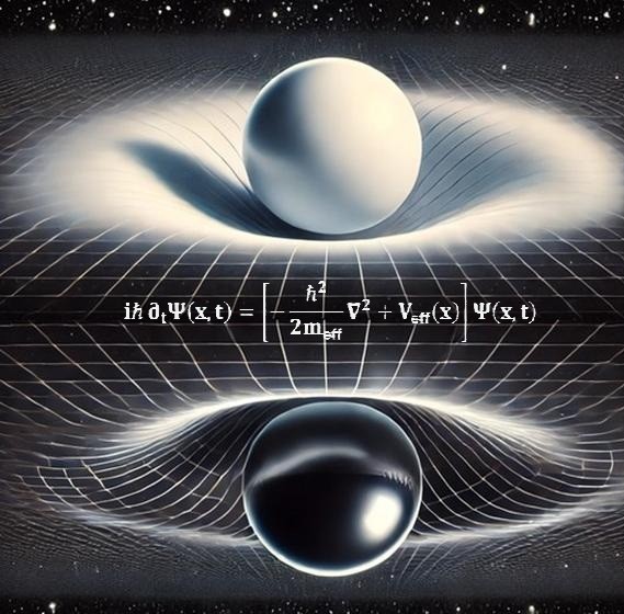
The Space–Time Membrane (STM) model proposes spacetime as a four-dimensional elastic membrane interacting with a parallel mirror domain. Every particle excitation on our “face” of the membrane has a corresponding mirror particle on the opposite face, ensuring exact matter–antimatter symmetry at the fundamental level and offering a possible route to addressing the observed baryon asymmetry. The membrane’s elastic dynamics simultaneously generate gravitational curvature and quantum-like phenomena: rather than postulating intrinsic randomness, apparent quantum probabilism emerges as a deterministic consequence of chaotic, sub-Planck elastic oscillations.
Gravity in STM. Transverse–traceless spin-2 excitations follow
with the identification . Time derivatives remain strictly second order. In the IR, the spin-2 bootstrap reproduces Einstein–; phenomenologically we obtain broadband inspiral phase shifts (), ringdown frequency shifts , and short-range Yukawa-type static corrections (symbols catalogued in Appendix Z).
UV control and EFT placement. Alongside these IR phenomenological aims, the refined STM model now has a complete UV control statement. In flat space and with vanishing open-system terms the quadratic Hamiltonian is positive and involves only , so no Ostrogradsky ghosts arise; the dominant sextic elasticity implies Lifshitz scaling with , under which the conservative interacting theory is super-renormalisable by power counting. Euclidean continuation yields reflection positivity for gauge-invariant composites and, via standard OS reconstruction, a positive spectral density. Finally, we state and use a decoupling/matching bound to Yang–Mills below a finite scale, which underwrites the SMEFT mapping employed later in the paper.
Concretely, the displacement field is decomposed into two complementary oscillatory modes that combine into a two-component spinor . Mode-by-mode interactions between each spinor component and its mirror antispinor redistribute energy—attractive interactions generate localised curvature (gravity), while repulsive or cancelling interactions reinject energy into the membrane background. Composite photons arise as coherent wave–anti-wave cycles. In the virtual (near-field) regime the energy exchanged in one half-cycle is returned in the next, so the period-averaged flux vanishes. By contrast, when the mode is on-shell—e.g. in an annihilation producing two photons—the same mechanism yields propagating gauge-like waves with positive cycle-averaged flux that carry away energy–momentum; the associated reduction in local strain/curvature equals the radiated energy.
When rapid sub-Planck oscillations in u are coarse-grained, a slowly varying envelope emerges that obeys an effective Schrödinger-like equation. This envelope reproduces interference patterns and apparent wavefunction collapse, recasting standard quantum phenomena (including the Born rule) as manifestations of deterministic chaos.
In this interpretation, Feynman’s path integral is re-expressed as a stationary-phase approximation to a single underlying wave field, rather than a literal sum over independently realised histories. The familiar kernel then appears as the WKB/multiple-scale approximation to STM’s Green function (Appendix D), providing a concrete, if still approximate, link between the membrane PDE and standard quantum-mechanical propagators.
The STM framework further reinterprets key aspects of particle physics. Electroweak symmetry breaking arises from rapid zitterbewegung-like interactions between spinors and mirror antispinors, generating and masses and yielding CP-violating phases without invoking extra scalar fields. A bimodal spinor decomposition underpins emergent gauge symmetries—U(1), SU(2) and SU(3)—as deterministic elastic connections.
The model incorporates:
- Scale-dependent elastic parameters and higher-order spatial derivatives (notably ) to regulate ultraviolet divergences.
- Non-Markovian memory kernels to explain deterministic decoherence and effective wavefunction collapse.
- A precise bimodal decomposition of u into a two-component spinor , yielding emergent gauge bosons.
- A deterministic electroweak symmetry-breaking mechanism via cross-membrane oscillations.
- A multi-loop renormalisation-group analysis and a nonperturbative scalar FRG study, revealing triple-well vacuum structure and elastic basins that can be used to model three fermion generations.
In the gravitational sector, linearised strain fields link directly to metric perturbations , yielding Einstein-like field equations from the STM action—even when including damping and scale-dependent couplings (Appendix M). A detailed multi-scale derivation (Appendix H) shows that coarse-grained sub-Planck oscillations produce a near-constant vacuum offset acting as dark energy [12,13], and that a mild late-time evolution in stiffness or damping could address the Hubble tension [14].
Crucially, Section 2.10—and the full parameter table in Appendix K.7—now fixes every STM coefficient to physical constants:
together with the vacuum-stiffness offset a macroscopic damping coefficient (corresponding to ), and the sextic regulator . These calibrations anchor the model quantitatively to the fundamental constants and , leaving no free elastic or damping parameters.
Although STM now captures both quantum-field and cosmological-scale phenomena within one PDE, several frontiers remain.
On the thermodynamics front, we have:
- Recovered the leading Bekenstein–Hawking area law via micro-canonical mode counting in the STM solitonic core (Appendix F.4), including estimates of finite-size corrections;
- Calculated grey-body transmission factors and effective horizon temperatures via fluctuation–dissipation (Appendix G.4–G.5);
- Sketched a Euclidean path-integral approach to the evaporation law, matching the leading-order timescale (Appendix H). Remaining thermodynamic tasks include subleading logarithmic and power-law corrections to the area law, Page-curve tests of unitarity and detailed first-law verifications (Appendix F.7).
Beyond thermodynamics, our analytic derivations (Appendices C and N) detail mode-by-mode spinor–antispinor couplings, while recent numerics anchored to physically motivated parameters reveal three well-separated mass minima that reproduce the Standard Model’s generational hierarchy, mixing angles and CP-violating phases (Section 3.1.4 & 4.3). Early tests (Section 3.3; Appendix K.7) suggested the damping coefficient might be dispensable, but a full analysis of measurement dynamics and deterministic wavefunction collapse (Section 3.4) confirms that a finite is essential. Although introduces mild non-conservatism, the model remains stable across a broad range of values.
Appendix T proves global well-posedness, self-adjointness and ghost-freedom, while Appendix U shows anomaly cancellation via mirror doubling. With these foundations in place, Appendix O now completes the spin–statistics link for STM’s bimodal spinor on globally-hyperbolic backgrounds; remaining frontiers are higher-loop renormalisation and the microstate structure of black holes.
Addressing the remaining challenges will be crucial to establishing the STM framework’s consistency across all scales.
Unlike many quantum-gravity schemes, the STM model is rooted in classical continuum elasticity, so it can be tested directly through numerical simulations and laboratory analogues such as metamaterials. By deriving Schrödinger dynamics, the Born rule, gauge symmetries and CP violation from a single deterministic PDE, STM uses far fewer independent postulates than frameworks of comparable scope—for example, the Standard Model plus general relativity, which require separate fundamental fields and symmetry assumptions. Approaches with an even sparser axiomatic core (e.g. asymptotically safe gravity) typically focus on the gravitational sector alone and do not yet reproduce the full gauge and flavour structure that STM aims to encompass.
We therefore encourage further numerical, experimental and theoretical exploration of the STM model as a promising, conceptually transparent route to reconciling quantum phenomena with gravitational curvature.
Organisation of the Paper
- Section 2 (Methods) provides a detailed overview of the STM wave equation, including explicit derivations of higher-order elasticity terms, spinor construction, scale-dependent parameters, and the deterministic interpretation of decoherence.
- Section 3 (Results) demonstrates how quantum-like dynamics, the Born rule, entanglement analogues, emergent gauge fields (, , ), deterministic decoherence, fermion generations, and CP violation naturally arise from the deterministic membrane equations.
- Section 4 (Discussion) explores the broader implications of these findings, along with possible experimental tests and numerical simulations.
- Section 5 (Conclusion) summarises the key theoretical advances, outstanding issues, and potential future directions, including proposals aimed at verifying the STM model’s predictions.
Appendices A–X comprehensively present supporting details, derivations, and numerical methods. They address:
- Operator Formalism and Spinor Field Construction (Appendix A)
- Derivation of the STM Elastic-Wave Equation and External Force (Appendix B)
- Gauge symmetry emergence and CP violation (Appendix C)
- Coarse-grained Schrödinger-like dynamics (Appendix D)
- Deterministic entanglement analogues (Appendix E)
- Singularity avoidance (Appendix F)
- Non-Markovian Decoherence and Measurement (Appendix G)
- Vacuum energy dynamics and the cosmological constant (Appendix H)
- Proposed experimental tests (Appendix I)
- Renormalisation Group Analysis and Scale-Dependent Couplings (Appendix J)
- Finite-Element Calibration of STM Coupling Constants (Appendix K)
- Nonperturbative analyses revealing solitonic structures (Appendix L)
- Covariant Generalisation and Derivation of Einstein Field Equations (Appendix M)
- Emergent Scalar Degree of Freedom from Spinor–Mirror Spinor Interactions (Appendix N)
- Spin–Statistics in the STM Framework (Appendix O)
- Reconciling Damping, Environmental Couplings, and Quantum Consistency in the STM Framework (Appendix P)
- Toy Model PDE Simulations (Appendix Q)
- CKM and PMNS flavour fits from an STM elastic template (Appendix R)
- STM Scattering Amplitude Validation (Appendix S)
- Well-Posedness and Ghost-Freedom of the STM PDE (Appendix T)
- Anomaly Cancellation in the STM Model (Appendix U)
- Effective Field Theory and Renormalisation Match for STM (Appendix V)
- Full SM-Gauge EFT (dim-6) and One-Loop RG (Appendix W)
- Causality (Non-Markovian) and Einstein– Bootstrap (Appendix X)
- UV structure, scaling and renormalisation, and a calibrated scalar FRG triple-well analysis (Appendix Y)
Finally, an updated Appendix Z serves as a Glossary of Symbols, ensuring clarity and consistency of notation throughout.
Scope and level of claim. It is important to stress what the present work does and does not establish. We do not claim a mathematically complete derivation of the Standard Model or a fully rigorous proof that quantum theory is redundant. Rather, starting from a single elasticity PDE we identify a set of consistent emergent structures — propagators, Schrödinger-type envelopes, gauge-like connections and flavour-mixing templates — and check them against selected experimental benchmarks. Within this scope we demonstrate a super-renormalisable elasticity field theory with Osterwalder–Schrader reconstruction and spin–statistics, an Einstein– limit for the transverse–traceless spin–2 modes, a calibrated scalar FRG triple-well analysis that underpins quantitative CKM/PMNS fits, and a minimal SMEFT bridge to collider observables. Several constructions (for example the solitonic FRG models of Appendix L and the non-Markovian master equations) are currently implemented in deliberately simplified truncations and geometries; by contrast, the scalar FRG analysis in Appendix Y.10 is anchored to the STM elastic coefficients and used quantitatively in our flavour fits. While non-trivial and quantitatively constrained in several sectors, the results should only be read as evidence that a deterministic membrane framework can plausibly reproduce key quantum and gravitational features, rather than as a finished, unique theory.
2. Methods
In the Space–Time Membrane (STM) model, spacetime is represented as a four-dimensional elastic membrane governed by a deterministic high-order partial differential equation. This single PDE unifies gravitational-scale curvature with quantum-like oscillations by incorporating higher-order elasticity, scale-dependent stiffness, non-linear terms, and possible non-Markovian effects. Below, we provide the theoretical foundations, outline the operator quantisation that yields quantum-like behaviour, show how gauge fields naturally emerge, discuss renormalisation strategies, and comment on the classical limit.
2.1. Classical Framework and Lagrangian
2.1.1. Displacement Field and Equation of Motion
We model the space–time membrane by a scalar displacement field , which encodes local departures from equilibrium. The canonical equation of motion is constructed so that each term has the dimensions of force per unit volume (N ). Higher-order elastic coefficients carry explicit powers of the Planck length where needed to keep SI units manifest. This equation is the master PDE from which all subsequent constructions are derived.
Canonical STM PDE (compact form).
The compact form derived in Appendix B is
Here collects the spatially uniform vacuum offset and any zero-mean local fluctuation . When fluctuations are not under discussion we write and may absorb it into . This expression suppresses explicit factors, which are absorbed into the higher-order moduli; it is the reference form used throughout the appendices.
The damping parameter is the mass-normalised rate (); the corresponding SI force-density coefficient is , which appears in the SI PDE as .
Explicit SI force-density form.
Restoring to make units manifest gives
Mass-normalised SI form.
Dividing by yields the form used for non-dimensionalisation and numerics:
with
and when fluctuations are retained. This is the form actually used for non-dimensionalisation and in the numerical solvers (Appendices K.6–K.7).
EFT sign-map.
The spectral identifications
are carried into the operator normalisations in Appendix V and Appendix W, so the signs of the derivative operators and the Wilson-coefficient conventions are consistent across the PDE, the emergent Lagrangian and the SMEFT translation (Appendix V §§V.1–V.2, Appendix W §W.2).
In what follows we use the compact (canonical) form; SI units are recovered by reinstating so that the and terms read and , with mass-normalised coefficients obtained by dividing by . The UV/renormalisation summary for the conservative sector appears in §2.4, with proofs in Appendix Y.
For gravitational notation we use , and as defined in Appendix Z and mapped to using §2.11 (tensor-mode EFT map) together with §2.1.1 (signs/units) and the conversion tables in Appendices K.6–K.7; the IR Einstein– completion is summarised in Appendix M.
Parameter summary.
For ease of reference we collect the main symbols, their roles, and the linear dispersion relation here.
Notation.is the baseline quartic stiffness, the spatially uniform vacuum offset, and zero-mean local fluctuations. Tildes () denote mass-normalised coefficients. We write for the Planck length, for spatial gradients, and for time derivatives. The emergent wave speed satisfies .
Key ingredients.
- : inertial density, fixed by matching dispersion to relativistic propagation.
- T: baseline tension, defines the emergent light-cone speed .
- : quartic stiffness, linked to the Newtonian gravitational sector.
- : vacuum offset, matched to the observed dark-energy density.
- : sextic regulator, set by the Planck-scale UV cut-off.
- (; damping rate): in SI force-density form the PDE carries ; after mass-normalisation this is . We distinguish a Planck-stage calibration rate (used only to set non-dimensional scales) from the laboratory/environmental rate obtained by ring-down of the same mode (if then ). Unless stated otherwise, in figures, fits and phenomenology means . The SI force-density coefficient is .
- : cubic nonlinearity, Higgs-like self-interaction.
- g: Yukawa/gauge coupling to spinor bilinears.
While not appearing explicitly in the scalar PDE, the spinor sector carries a milder dephasing that enters the Dirac-like equations for the spinor and mirror-spinor fields. Coarse-graining ties it to the scalar damping so that flavour decoherence occurs on the same physical timescale as scalar Born-rule collapse:
(see §3.4.1 and Appendix K.6).
Dispersion (linear, mass-normalised).
For plane-wave solutions and the rule , the linearised dispersion relation is
For we have : exponential decay, as expected for physical damping. With , the quadratic energy is positive and the linear operator is sectorial (Appendix T), ensuring well-posedness and the absence of higher-derivative ghosts in the second-order-in-time formulation.
This PDE therefore provides a unified mathematical context in which large-scale curvature emerges as low-frequency deformations and short-scale oscillations mimic quantum phenomena—without extra dimensions or intrinsic randomness.
2.1.2. Lagrangian Density
The elastic dynamics follow from a local Lagrangian density . Damping and external work are handled via a Rayleigh dissipation functional and an explicit forcing term, rather than being placed inside the conservative Lagrangian. As in §2.1.1, the compact (canonical) form suppresses explicit powers of the Planck length ; the SI-expanded form reinstates them so that every Euler–Lagrange term has units of force per unit volume (N ).
Canonical (compact) Lagrangian density.
Variation of the action built from reproduces the conservative part of the canonical STM PDE in §2.1.1 (i.e. without damping and ).
Explicit SI form (higher-order pieces with).
Writing the quartic and sextic operators with explicit Planck-length factors,
For covariant discussions we use a split and write the quartic term in terms of the spatial Laplace–Beltrami operator ; time evolution remains second order, while higher-order operators act on space alone (Appendix T). With the and insertions, each Euler–Lagrange term carries SI units N (Appendix K.6), matching the force-density PDE in §2.1.1.
Rayleigh dissipation (damping).
Damping is introduced via a Rayleigh functional
Here is the mass-normalised rate (); the corresponding SI force-density coefficient is , which appears in the SI PDE as . In the Euler–Lagrange–Rayleigh equation, enters on the right-hand side; moving it to the left reproduces precisely the term in §2.1.1.
Mass-normalised density (solver form).
Dividing by gives the mass-normalised Lagrangian density
with
In this normalisation, damping corresponds to
and the Euler–Lagrange–Rayleigh equation yields the mass-normalised PDE
in place of , in agreement with §2.1.1 and Appendices B, K, P, Q and T. This mass-normalised form is the starting point for the non-dimensionalisation used in Appendices K.6–K.7.
Assumptions for linear analysis.
For the linear theory we assume
and the nonlinear terms are locally Lipschitz on . These conditions match those used in Appendix T (Thm T.1, Prop. T.2) and underpin the well-posedness and ghost-freedom statements quoted in §2.4.
2.1.3. Hamiltonian Formulation and Poisson Brackets
The Hamiltonian density follows from a Legendre transform of the conservative Lagrangian; Rayleigh damping and external work enter only as generalised forces and do not contribute to the Hamiltonian.
Canonical momentum.
Hamiltonian density.
(In SI-expanded form, insert and on the and pieces exactly as in § 2.1.2.)
Canonical brackets.
Hamilton’s equations, , , reproduce the conservative STM dynamics; energy decay arises solely from the Rayleigh term:
A rigorous curved-spacetime proof of self-adjointness, ghost-freedom and global well-posedness is given in Appendix T (Thm T.1; Prop. T.2). The BRST-compatible open-system implementation of damping appears in Appendices P and T (Thm T.6).
Energy flux (Noether). For spatial translations, the conservative energy density and flux obey the local continuity law
A convenient symmetric representative, consistent with the elastic operator , is
This closes the continuity equation for the conservative field equation
Units. .
Mass-normalised flux
Dividing by and writing , , ,
with (specific energy flux).
With damping and forcing
Including Rayleigh damping and external work, the local balance becomes
and the control-volume balance over Vis
Ifvaries in space–time
When is not constant, spatial translation invariance is broken by the explicit coefficient dependence, and the conservative continuity law acquires source/sink terms:
Thus strict conservation holds whenever is constant (or at least and ).
2.1.4. Conjugate Momentum and Dispersion
Conjugate momentum. From the conservative Lagrangian density of §2.1.2 the canonical momentum is
Rayleigh damping contributes only as a generalised force; it is not part of the conservative Hamiltonian.
Mass-normalised linear PDE. Dropping nonlinearity, spinor coupling and forcing, and dividing the SI equation by , the linearised STM equation with physical damping reads
With
Dispersion relation. Insert a plane wave and use . One obtains
or, equivalently (multiplying by ),
Thus for : physical exponential decay. The positive signs , , correspond to a positive quadratic energy and a sectorial generator (see Appendix T).
Coherence note (envelope visibility).
In interference estimates it is convenient to collect dephasing/inhomogeneous broadening into an effective transverse rate
so the propagation decoherence length is
with the group speed extracted from the dispersion. For slit–screen time of flight , the visibility decays as
which reduces to in the baseline STM (no extra spinor dephasing and negligible inhomogeneity).
Interpretation and limits.
Inertia gives ; damping contributes .
fixes the emergent light-cone speed; and stiffen the spectrum, with the sextic piece suppressing short-wavelength growth and bounding the UV.
Long-wavelength : . High-k limit: . Weak damping : conservative dispersion with a small imaginary correction.
When is non-negligible or periodic, the plane-wave analysis is replaced by the numerical framework of §2.5/Appendix K, or by a Bloch-type treatment for band structure.
Numerics hook (sign/unit fidelity). All solvers (Appendix Q) implement the linear spectral stencil
which exactly matches the mass-normalised PDE above.
When modelling coherence/visibility rather than field amplitude, fold additional channels into and apply the factor (temporal) or (spatial).
Propagator conventions and boundary prescriptions for L are collected in § 2.1.5. The envelope (Schrödinger) and path-integral structures derived from the same operator appear in § 3, with multi-scale details in Appendix D and open-system/response links in Appendices G and T.
2.1.5. Propagators and Response Functions (Linearised STM).
We fix propagators as inverses of the linearised STM operator defined in § 2.1.1–2.1.4. We take , so and .
Retarded/response. The retarded Green function solves
For homogeneous coefficients the frequency–wavenumber form reads
Optionally, in mass-normalised variables (divide by ):
For small , each simple pole lies at with .
Time-ordered, Euclidean, and Keldysh.uses the prescription; the Euclidean/Matsubara version follows . For non-equilibrium we use the Schwinger–Keldysh triplet , with fixed by fluctuation–dissipation in equilibrium.
Inhomogeneity and boundaries. If parameters vary spatially, write ; then with ; contour choice fixes causality.
Spectral representation and stability.
Positivity and sum rules provide checks/identifications.
Envelope connection. The Schrödinger-type envelope kernel Ais not the same object as , but shares small- pole data (group velocity, curvature/diffraction, attenuation via ), bridging membrane waves to envelope dynamics.
Notes on symbols. Here is Rayleigh damping (mass-normalised form used in § 3.1.1); g denotes the Yukawa/gauge coupling (not a scalar “gap”); ℏ is the usual reduced Planck constant.
2.2. Operator Quantisation
2.2.1. Canonical Commutation Relations
As in § 2.1.3, quantisation applies to the conservative Hamiltonian sector; the damping and forcing terms arising from the Rayleigh functional are excluded and play no role in the commutator structure.
Building on the Hamiltonian structure just introduced, we promote the displacement field and its conjugate momentum a to operators and on a suitable Sobolev domain. The classical Poisson bracket
is elevated via the Dirac correspondence
which immediately yields
with all other commutators vanishing. Thus the non-commutativity of and emerges naturally from the membrane’s intrinsic symplectic form, without requiring an extra quantisation postulate.
Spin–statistics. Equal-time CAR for the bimodal spinor are not assumed here; they are derived in Appendix O from locality, microlocal/Hadamard positivity and normal hyperbolicity, with stability under small, local BRST-compatible GKSL deformations.
2.2.2. Normal Mode Expansion
In nearly uniform regions, one may write
The associated Hamiltonian sums over the modes, each with a modified dispersion . When varies, a real-space diagonalisation or finite element approach is more suitable. Either way, the operator quantisation ensures a “quantum-like” spectrum of excitations that parallels bosonic fields in standard quantum theory.
2.3. Gauge Symmetries: Emergent Spinors and Path Integral
2.3.1. Bimodal Decomposition and Emergent Gauge Fields
A distinctive aspect of the STM model is constructing a bimodal decomposition of . Formally, one splits u into two complementary oscillatory components, sometimes referred to as in-phase and out-of-phase fields:
and arranges into a two-component spinor . Imposing a local phase invariance necessitates the introduction of gauge fields, e.g.\ for . Extending this principle can yield non-Abelian fields and , reproducing the main gauge bosons familiar from the electroweak and strong interactions [15, 16].
Mechanically, each gauge field arises as a compensating “connection” ensuring that local redefinitions of the spinor field do not alter physical observables. Consequently, photon-like or gluon-like excitations appear as coherent wave modes in the membrane. In standard quantum field theory, “virtual particles” mediate interactions; here, such processes correspond to deterministic wave–anti-wave cycles wherein net energy transfer over a full cycle is zero, aligning with the virtual-exchange picture. By including local phase invariance in the STM action, one automatically generates covariant derivatives (or the non-Abelian analogue), reinforcing how gauge fields naturally emerge from the underlying elasticity.
In the path-integral language, enforcing local spinor symmetries introduces these gauge connections and ghost fields (for gauge fixing) but does not rely on intrinsic randomness. Instead, it unites the deterministic elasticity framework with internal gauge invariance. This places photon-like excitations (for U(1)), bosons (for SU(2)), and gluons (for SU(3)) as collective membrane oscillations that preserve local symmetry at each point in spacetime.
2.3.2. Ontology of Non-Abelian Gauge Fields
In STM the familiar non-Abelian gauge symmetries SU(2) and SU(3) arise in exactly the same way as U(1), only now acting on higher-dimensional internal oscillator spaces. Concretely:
SU(2) as Local Doublet Rotations
At each spacetime point the STM spinor is promoted to a two-component doublet . The internal freedom to rotate
corresponds to choosing a new basis in the two-mode oscillator plane.
To compare and without ambiguity we introduce the matrix-valued connection , so that the covariant derivative remains well-defined under local SU(2) rotations.
Physically, each generator of SU(2) is realised as a distinct “twist” or shear of the STM membrane’s two-mode oscillation, and the Yang–Mills field strength measures the membrane’s curvature in that internal rotation space.
SU(3) as Local Triplet Rotations
Similarly, for colour we carry a three-component oscillator transforming under local SU(3) rotations .
An eight-component connection (with the Gell-Mann generators) compensates infinitesimal changes in that three-mode orientation, yielding .
The associated field strength is nothing but the elastic-energy cost of non-commuting shears in the membrane’s colour-triplet oscillation bundle.
Unified Membrane Interpretation
In every case, gauge symmetry is simply the freedom to rotate the internal oscillator basis at each point in a way that costs elastic energy when misaligned.
All familiar Maxwell or Yang–Mills Lagrangians arise from writing down the membrane’s elastic energy as the square of these curvature two-forms.
Thus, U(1), SU(2) and SU(3) gauge fields share a single ontological origin: the tangent-space rotations of the STM membrane’s multimode oscillations.
No mandatory high-energy convergence
Because U(1), SU(2) and SU(3) all arise as different rotational polarisations of the same four-dimensional membrane, their common origin is already encoded in the Lagrangian. The usual grand-unification requirement at some ultra-high scale is therefore optional, not obligatory. Functional-RG trajectories in Appendix J show that for some stiffness ratios the three couplings can approach one another near the sextic fixed point, but nothing in the STM dynamics enforces that coincidence. Hence proton-decay bounds do not constrain STM, and the model accommodates either convergent or non-convergent running without additional fields.
Path-integral viewpoint.
For calculations, the emergent gauge sector can be handled in the usual BRST-fixed path integral,
2.3.3. Virtual Bosons as Deterministic Oscillations
In standard quantum field theory, “virtual particles” are ephemeral excitations in Feynman diagrams. Here, such processes are reinterpreted as energy-balanced wave–plus–anti-wave cycles. Over one period the cycle-averaged energy flux through any closed surface vanishes, consistent with a virtual (near-field) exchange:
so the membrane’s local elastic/curvature energy is borrowed and returned within each cycle, rather than being dissipated or radiated.
By contrast, on-shell (far-field) emission — e.g. an annihilation on our face producing two photons — carries positive cycle-averaged flux,
and the associated decrease of local strain/curvature equals the radiated energy (up to small damping losses). There is therefore no double counting: energy that leaves as real radiation is not simultaneously assigned to a separate “curvature-relief” reservoir. Bound-state shifts (e.g. Lamb-like) are computed from the coarse-grained Hamiltonian density.
Equivalently, with the total STM+gauge energy density and Sits Noether/Poynting-like flux, the balance in a fixed control volume Vis
Near field: the surface term averages to zero over one period; far field: it does not.
2.4. UV Structure and Power Counting
We summarise the UV properties proven in Appendix Y. In the conservative limit () the linearised STM Lagrangian yields and a positive quadratic Hamiltonian; higher derivatives are purely spatial, excluding Ostrogradsky modes. The dispersion implies in . With and , local scalar and Yukawa couplings carry positive mass dimension and the superficial degree of divergence obeys , so only the elastic set and a finite number of relevant interaction normalisations renormalise. Gauge-invariant composites satisfy reflection positivity and admit a Källén–Lehmann representation; a gauge-covariant gradient flow provides a non-perturbative definition of renormalised local operators. Below a matching scale the STM gauge-invariant Schwinger functions agree with Yang–Mills up to ; this underwrites the SMEFT bridge used in Apps. V–W.
2.5. Renormalisation and Higher-Order Corrections
2.5.1. One-Loop and Multi-Loop Analyses
The sixth-order operator ensures strong damping of high-momentum modes, so loop integrals converge more rapidly than in a naive second-order theory. Standard dimensional regularisation and a BPHZ subtraction scheme can be applied to compute self-energy corrections at one-loop or higher orders (see Appendix J). The resulting beta functions typically take the schematic form:
where are integrals influenced by and factors in the propagator. Multi-loop diagrams, including “setting sun” or mixed fermion–scalar topologies, refine these flows further. Crucially, running elastic couplings and can exhibit non-trivial fixed points, opening the door to multiple stable vacua or discrete mass spectra.
Nonperturbative FRG and Solitons
Perturbation theory alone cannot capture phenomena like solitonic black hole cores or multiple vacuum states. Thus we employ Functional Renormalisation Group (FRG) methods in two complementary sectors: a calibrated scalar analysis for the STM elastic potential (Appendix Y.10) and a deliberately simplified FRG-plus-soliton toy model (Appendix L), both tracking an effective action as fluctuations are integrated out down to scale k. These flows can reveal topologically stable solutions (e.g. kinks, domain walls) and non-trivial vacuum structure which are crucial for:
- Fermion generation: In the calibrated scalar sector (Appendix Y.10) an open set of STM-anchored UV couplings flows to an effective triple-well potential at a finite infrared scale; the three resulting elastic basins define distinct, well-separated mass scales, paralleling the three observed fermion generations and feeding the flavour templates of Appendix R.
- Black hole regularisation: Enhanced stiffness from and stops curvature blow-up, replacing singularities with finite-amplitude standing waves.
2.6. Classical Limit and Stationary-Phase Approximation
In a classical or macroscopic regime, one sets or assumes heavy damping. The path integral
is dominated by stationary-phase solutions of the PDE. Thus, the membrane behaves as a purely classical object with fourth- and sixth-order elasticity. Conversely, at sub-Planck scales—where the chaotic interplay of and acts—coarse-graining these rapid oscillations yields interference, Born-rule-like probability patterns, and gauge bosons as emergent wave modes (Appendix D).
Thus the familiar Schrödinger equation and its path-integral form are simply calculational devices—valid envelope approximations to our single, deterministic STM wave equation—rather than fundamental postulates of nature.
2.7. Non-Markovian Decoherence and Wavefunction Collapse
Although the STM PDE is fully deterministic, real-world observations exhibit effective wavefunction collapse. In STM this emerges from non-Markovian decoherence. We split the field into slow (“system”) and fast (“environment”) components, integrate out the fast sector on a closed-time-path (Schwinger–Keldysh) contour, and obtain a Feynman–Vernon influence functional [19]. The reduced state of the slow component then satisfies an integro-differential memory-kernel master equation. Off-diagonal elements in the pointer basis decay deterministically due to the finite correlation time of the eliminated modes, reproducing apparent measurement collapse without introducing fundamental randomness. In the Markov limit (short memory) the kernel reduces to a GKSL form with dephasing rate (as in §§2.1.1–2.1.4), and the construction is BRST-compatible (Appendix T.6).
This same non-Markovian structure supports deterministic entanglement analogues (Appendix E): CHSH-type violations arise at the coarse-grained level via contextual, measurement-dependent correlations seeded by the shared preparation and finite-memory channel (see §3.4.4), while preserving locality of the underlying PDE and no-signalling. The rate and mechanism of decoherence are, in principle, testable in laboratory analogues and metamaterial platforms (Section 4.1; Appendix I).
2.8. Persistent Waves, Dark Energy, and the Cosmological Constant
In the long-wavelength, low-frequency limit , the full SI STM equation
reduces because the and operators are suppressed by factors and . The surviving SI balance is
and, dividing by ,
Both terms in the SI form carry units of force per unit volume (since and ). After division by , every term has units of acceleration .
The slow, mirror-induced modulation of the quartic stiffness,
does not appear as a zero-derivative “mass term” in the wave equation. Rather, it enters the energy balance through the contribution to the energy density . When varies slowly, the local balance (§2.1.3) reads
so phase-locked persistence of the standing/interference pattern comes from the parametric input balancing Rayleigh loss in the near field (where the surface flux averages to zero over a cycle). The spatially uniform component that survives coarse-graining acts as a tiny, slowly varying stiffness offset on large scales (H.4) and maps onto in the IR Einstein– sector (see T.2); there is no double counting with (§2.8/T.2 note).
Units note.
- In SI equations of motion: (force density).
- In energy density : (pressure).
- Planck factors appear only with higher-order terms in SI: multiplies and multiplies ; the term has no factor.
A “Eureka” reinterpretation of the double-slit
Persistent waves via modulated stiffness
Treating the double-slit fringes as persistent elastic standing/interference waves immediately poses a puzzle: with Rayleigh damping present, such waves cannot survive without a gentle, phase-locked trickle of energy. In STM this persistence arises because rapid mirror exchange (App. P) induces a small, slow modulation of the effective quartic stiffness,
which acts as a parametric feedback that phase-locks the oscillations and compensates the Rayleigh loss. In near-field (virtual) exchange the cycle-averaged radiative flux vanishes, so the tiny input from -modulation is what keeps the pattern alive without net radiation.
At the level of energy balance (§2.1.3), a space–time dependent adds a source term. Locally,
so in a steady, near-field periodic state (no net surface flux, ) the time-averaged parametric input balances damping:
The uniform component that survives coarse-graining acts as a tiny, slowly varying stiffness offset on large scales, providing the same discussed in T.2 (no double counting with ; see §2.8/T.2).
B Emergent cosmological constant
The strain-to-curvature map of Appendix M.6 identifies the constant offset with a vacuum-energy term
Because , an imperceptible fractional shift
reproduces the observed dark-energy density . Thus STM links quantum interference and cosmic acceleration without introducing extra fields or stochastic postulates.
A full spin-2 bootstrap showing that these assumptions yield Einstein’s equations with a cosmological constant appears in Appendix X §X.2.
C Ultraviolet safety and solitonic cores
At large strain the sextic regulator dominates, raising the effective stiffness and preventing divergences. Appendix M.7 shows this caps curvature inside collapsing regions, replacing general-relativistic singularities with finite-energy solitonic cores that still satisfy .
D Numerical window
Even with , quartic and sextic terms re-enter at LIGO-band strains (), far above laboratory scales yet well below the Planck modulus—ensuring consistency from tabletop interferometers to gravitational-wave astronomy.
In essence. A single eight-parameter elasticity law explains persistent quantum fringes, an effective cosmological constant, and singularity avoidance. The eureka insight—that double-slit coherence demands a mirror-induced, additive stiffness modulation—turns out to be the same ingredient that could drive the Universe’s late-time acceleration.
2.9. Action Principle in Curved Spacetime
2.9.1. Action Principle
We embed the STM framework on a four-dimensional Lorentzian manifold by introducing a single action
where R is the Ricci scalar of the metric . The STM Lagrangian splits into three parts:
- the scalar “membrane” sector ,
- the two-component spinor sector , and
- their elastic interaction .
All ordinary derivatives are replaced by Levi–Civita covariant derivatives, and each elastic constant enters as a diffeomorphism-invariant scalar. In particular, we define
2.9.2. Field Equations
Varying S with respect to yields the Einstein equations with an STM stress–energy tensor:
Variation with respect to the scalar field gives a covariant sixth-order membrane equation:
Variation with respect to produces the curved-space Dirac equation with nonlinear coupling:
2.9.3. Flat-Space and WKB Limits
By specialising , replacing and taking the semi-classical (WKB) limit, one recovers:
- the sixth-order scalar membrane PDE;
- the nonlinear Schrödinger-like envelope equation with STM coefficients;
- the elastic spinor–scalar coupling driving unseeded spinor emergence.
Thus the covariant formulation reduces exactly to the flat-space STM model under the appropriate limits.
2.10. Physical Calibration of STM Elastic Parameters
Even though the STM equation is written in dimensionless form, its coefficients must reproduce familiar physical constants when reinstated with units. The table below summarises each STM symbol, its calibrated SI value, and the physical anchor (derivation given in Appendix K.7):
| STM symbol | Value (SI) | Anchor |
| T | ||
| Quartic stiffness (coefficient of in SI force-density form) | GR matching for the quartic operator. | |
| observed | ||
| UV cut off | ||
| g | ||
| Higgs quartic * | ||
| (coefficient of the term) | Planck-time decoherence | |
* Calibrated to the magnitude of the SM Higgs quartic to set the symmetry-breaking scale in the effective low-energy sector. This is not a claim of a fundamental Higgs field in STM: electroweak masses arise from deterministic face–mirror zitterbewegung and gauge-sector dressing (see §2.3 and App. C.3.1), withacting as an emergent elastic proxy that fixes the infrared scale. In explicit SI force-density form the higher-order terms areand; do not quotein Pa in tables—quotein N.
These eight calibrated coefficients—, T, , , , g, , and —anchor the STM model quantitatively to c, G, , and the Planck scales, yielding a fully testable system of dimensionless parameters for use in Section 3 and 4. The same sign choices ensure positivity/sectoriality in the conservative UV analysis (§2.4; App. Y).
When reporting SI coefficients, list (N) rather than (Pa). Provide or as appropriate for spatial-propagation fits.
2.11. Tensor-Mode EFT Mapping (STM → GR with Soft UV Corrections)
In this subsection we isolate the transverse–traceless tensor sector of STM and present a minimal effective-field-theory (EFT) mapping to a GR-like graviton with soft UV corrections. The goal is to provide a clean dictionary between the STM elastic coefficients and the usual graviton EFT parameters, not to claim a full derivation of general relativity from STM.
Sign choices and parameter map.
We work with the same sign conventions as in §2.1.1 and §2.4 and assume
In the tensor sector we identify
with under IR Lorentz restoration (solver/SI conversions as in App. K.6–K.7).
In the explicit-SI PDE of §2.1.1 the quartic piece is , so the mass-normalised SI coefficient is
and one may equivalently write . In what follows are dimensionless EFT parameters expected to be , while encodes the effective UV scale of the tensor sector.
Minimal graviton EFT (closed/unitary sector).
Restricting to transverse–traceless (TT) modes on a GR background, the linearised STM tensor sector is second order in time and higher order in space. A convenient EFT parametrisation of the TT dispersion relation is
which carries no extra polarisations and no higher-time derivatives (so no Ostrogradsky ghosts).
In this language:
- the term reproduces GR’s massless graviton in the IR;
- the and pieces encode STM’s quartic and sextic stiffness as soft UV corrections;
- observable consequences appear as small modifications to gravitational-wave dispersion/phasing, static weak-field tails and black-hole ringdown spectra.
Appendix M gives the Einstein-like mapping in more detail and §M.12 quotes the corresponding phenomenological scalings.
Static weak-field potential.
In the static, weak-field limit the tensor-mode EFT reduces to a modified Poisson equation for the potential :
Solving this with the sign choices above yields the standard Newtonian term
plus short-range Yukawa and/or oscillatory corrections, whose ranges and relative weights are fixed by the roots of the characteristic polynomial
These corrections are controlled by the same that enter the graviton dispersion; they therefore provide an independent way to constrain and via laboratory and Solar-System tests of gravity.
Scope of the mapping.
The dictionary above applies to the closed, linear TT sector and assumes that scalar and vector perturbations are either non-propagating or heavy/screened at the scales of interest. Non-linear back-reaction, strong-field effects and possible scalar-tensor mixings are treated in Appendix M and in the black-hole analysis of Section 4.7; here we restrict ourselves to the minimal tensor-mode EFT needed for dispersion, near-field and ringdown phenomenology.
2.12. Summary of Methods
We start from a single high-order elastic wave equation for the membrane displacement u, incorporating scale-dependent stiffness, fourth- and sixth-order spatial derivatives, linear damping, cubic non-linearity, Yukawa-like coupling to emergent spinors and external forcing.
Canonical quantisation promotes u and its conjugate momentum to operators in a suitable Sobolev space, with self-adjoint Hamiltonian terms up to . All eight coefficients are calibrated once to and the Planck scales (table in §2.10; App. K.7); thereafter, no additional elastic or damping parameters are tuned in the predictions reported here. In the IR, the spin-2 bootstrap (App. X.2) shows that STM’s two-derivative gravitational sector closes uniquely to Einstein– with matter stress–energy supplied by the emergent spinors.
A bimodal decomposition of u yields a two-component spinor field; imposing local phase invariance generates U(1), SU(2) and SU(3) gauge fields.
A multiple-scale (WKB) expansion separates fast sub-Planck oscillations from a slow envelope, giving an effective Schrödinger-like equation whose interference, Born-rule density and decoherence follow deterministically once is included (see Section 3.4).
Functional and perturbative renormalisation analyses exploit the term to tame UV divergences, reveal non-trivial fixed points (fermion generations) and support solitonic cores (singularity avoidance).
The model is immediately testable through a Mylar-membrane interferometer whose geometry fixes the quartic stiffness/propagation coefficient by design, leaving the mass-normalised damping as the sole exported laboratory parameter (see App. I.2). This single number calibrates flavour dephasing and informs gravitational-wave amplitude analyses ; consequently, a Mylar measurement or bound on propagates directly to tighter cross-sector constraints (see App. I.6)
3. Results
This section presents the principal findings of the Space–Time Membrane (STM) model.
Throughout this section we work in the near-paraxial, small-amplitude regime of the linearised operator L, with quasi-monochromatic carriers , slowly varying coefficients , and a clear carrier–envelope scale separation; all envelope and path-integral statements are at leading non-trivial order in these parameters. We use the operator, Fourier and damping conventions fixed in § 2.1.5 throughout Section 3.
Gravitational-wave and static predictions use the tensor-mode parameterisation introduced in §2.11, with IR Einstein– behaviour supplied by Appendix X/M.
We begin by examining perturbative results, illustrating how quantum-like dynamics, gauge symmetries, and deterministic decoherence arise from a high-order elasticity framework. We then turn to nonperturbative effects, whose full derivation—via the Functional Renormalisation Group (FRG)—appears in Appendix L.
3.1. Perturbative Results
3.1.1. Emergent Schrödinger-Like Dynamics and the Born Rule
We start from the mass-normalised STM equation of motion (see §2.1.1):
where , , , and is the calibrated damping (Appendix K.7). (SI force-density form has ; after dividing by this becomes .)
With the conventions of § 2.1.5, the linearised dispersion is
so damping is strictly stabilising (Appendix T).
Envelope/WKB reduction. By coarse-graining the rapid, sub-Planck oscillations in , one obtains a slowly varying “envelope” . Specifically, one applies a smoothing kernel (often Gaussian) and adopts a WKB-type ansatz,
and expanding (3.1) order-by-order separates into a Hamilton–Jacobi equation for S and a continuity equation for A. Using the operator, Fourier and damping conventions of § 2.1.5, the near-paraxial coarse-graining yields the envelope law stated below. At leading order the slow envelope obeys an effective Schrödinger equation,
where and are fixed combinations of and the slow background; the term controls the UV through its contribution to those coefficients (details in Appendix D). The small positive is the calibrated, mass-normalised damping (), entering here as a linear attenuation of the envelope.
Born rule and determinism. With , the envelope dynamics contract onto measurement-defined attractors, and realises the Born weights via deterministic sub-Planck chaos (Section 3.4; Appendix P). Thus STM reproduces interference and outcome statistics without intrinsic randomness [20].
While this deterministic approach now reproduces the Born rule and approaches the Tsirelson bound, it still departs conceptually from the mainstream view that quantum indeterminism is fundamental. Rigorous loop-level checks (e.g. chiral anomalies) and targeted experiments — such as ultra-long interferometry or fast-switch Bell tests that probe the finite memory time predicted by the STM kernel — are needed to confirm whether the model matches standard quantum mechanics at all scales.
3.1.2. Uncertainty Relations from STM
Fourier/kinematic route. Any STM wave-packet obeys . With for the envelope’s canonical pair (Appendix D), this gives
Canonical/commutator route. The envelope action carries the symplectic term , hence and the same bound .
Time–energy. With small mass-normalised damping , the retarded pole has width , so and therefore . (See the dispersion and damping sign already established in § 2.1/§ 2.1.5 and used in § 3.1.1.)
Pipeline Rosetta Flow
STM PDE (§ 2.1) → invert (choose contour) → propagators /Keldysh ; STM PDE → multi-scale/WKB → envelope (Schrödinger); envelope → integrate out fast modes → effective action → path-integral kernel K.
3.1.3. Emergent Gauge Symmetries
A hallmark of STM is that gauge structure emerges from the bimodal decomposition of the displacement field . Writing the two slow envelopes as and assembling them into a two-component spinor , we impose local phase covariance on , which forces gauge connections via minimal coupling.
Abelian case (U(1)). Under a local re-phasing
covariance of the envelope dynamics requires
with a Maxwell term in the emergent Lagrangian and conserved current .
Non-Abelian extension. Demanding local symmetry in the internal mode space and colour space yields the Yang–Mills structure
with the standard field strengths. In this reading, photon-, - and gluon-like excitations are coherent membrane modes (collective waves) rather than stochastic quanta [16]. Processes usually described as “virtual boson exchange” are reinterpreted as wave–plus–anti-wave cycles that exchange phase/momentum while averaging zero net energy over a cycle (cf. § 2.1.2, Appendix P).
Analogies (intuition building).
- Electromagnetism as phase connection. The U(1) potential plays the role of a geometric “connection” that keeps the local phase of the two-mode envelope aligned across the membrane—exactly as a classical bundle connection aligns phases along a fibre [16].
- Strong force as a lattice of coupled oscillators. Visualising the membrane as a lattice of linked oscillators, each site carrying an effective “colour, ” the elastic coupling stiffens with separation, producing a linearly rising energy cost and hence confinement; gluon-like modes are the coherent waves on those links [15].
- Virtuals as counter-oscillations. Internal lines in Feynman graphs map to counter-propagating wave pairs whose instantaneous energy budget is balanced over a period, preserving exact energy conservation while reproducing the same effective interactions.
Electroweak breaking (deterministic mechanism). When a uniform background displacement is present and face–mirror couplings are switched on, rapid zitterbewegung between and its mirror partner (§ 3.7) generates effective mass terms for the weak gauge fields, mimicking electroweak symmetry breaking without positing a fundamental scalar at the microscopic level. The constructive details and parameter map are given in Appendix C.3.1.
Formal consistency: anomalies and damping.
- Anomaly cancellation. Appendix U proves that mirror doubling renders the chiral spectrum vector-like, so all perturbative gauge, mixed and gravitational anomalies cancel on any globally-hyperbolic background; BRST nilpotency is preserved.
- BRST-compatible dissipation. The small Lindblad terms used for damping/dephasing commute with the BRST charge (or are BRST-exact), so the physical cohomology is preserved under open evolution (Appendix T, Thm. T.6), consistent with the dissipator choices in § 3.4 and Appendix P.
Empirical touchstone. The emergent gauge Lagrangian reproduces the tree-level differential cross-section, including –Z interference and one-loop leptonic running (Appendix S; Scattering_amplitude.py). This anchors the correspondence beyond formal symmetry.
Data-facing bridge. For comparisons beyond tree-level , Appendix V provides a compact STM→SMEFT dictionary (including , , ) and Appendix W extends this to the full set with one-loop running to and the oblique mapping. These let global-fit bounds be translated directly into STM parameter inequalities.
Scope and next steps. With U(1)×SU(2)×SU(3) realised and anomaly freedom secured, full equivalence with the Standard Model requires extending tests to non-Abelian multi-leg processes and loop corrections; those (together with the effective-scalar channel of Appendix C) are the next targets.
Result (Appendix O). In the conservative limit, scalar/membrane observables commute at spacelike separation (CCR), while the bimodal spinor obeys CAR and anticommutes at spacelike separation; the graded locality persists for under local BRST-compatible GKSL deformations.
Computational note. A practical realisation of the elastic–spinor coupling, constraint preservation, and the GKSL step used in our solvers is given in §3.1.4 (see also Appendix P; Appendix T, Thm. T.6).
3.1.4. Deterministic Decoherence and Bell-Inequality Violations
Splitting the displacement field into slow “system” and fast “environment” components, , and integrating out with a Feynman–Vernon influence functional (Appendix G) yields a non-Markovian master equation for the reduced state :
where the memory kernel K encodes finite bath correlation times and is a quadratic superoperator fixed by the STM couplings and the coarse-grained bath statistics. In the short-memory limit (Appendix P), the kernel reduces to a GKSL/Lindblad form that is BRST-compatible on curved backgrounds (Appendix T, Thm. T.6), ensuring positivity and preservation of the physical subspace.
Measurement and collapse (deterministic). The small but fixed Rayleigh damping in the scalar sector (mass-normalised form) induces envelope-level dephasing of the emergent spinor channels at rate (Appendix K.6–K.7, § 3.4). With spinor-based measurement operators (e.g. ), the ensuing dynamics deterministically drive the state to one of the measurement basins (Appendix E), without stochastic postulates.
Bell correlations from internal phase. Each spin packet carries a fixed internal phase between its two elastic modes; a Stern–Gerlach analyser at angle projects that phase onto its eigen-basis. The coincidence curve
follows as squared overlaps (derivation in Appendix E.3). For two analysers at angles , the correlation is , and the CHSH parameter reaches , [20, 21] violating the classical Bell bound while arising from a deterministic PDE with finite-memory dissipation.
Caveat and targets. Laboratory environments are often near-Markovian; quantitative comparison of STM-predicted decoherence times and memory kernels with experiment (including environment-induced superselection) remains an open programme. The curved-space, BRST-compatible dissipator used here guarantees complete positivity and gauge compatibility (Appendices P, T), anchoring those comparisons on a self-consistent foundation.
3.1.5. Fermion Generations, Flavour Dynamics, and Confinement
Discrete vacua from RG flow. Combining the perturbative running of the elastic couplings (Appendix J) with a calibrated scalar FRG analysis (Appendix Y.10) shows that an open set of STM-anchored ultraviolet couplings flows to an effective triple-well potential at a finite infrared scale. The three resulting elastic basins provide distinct, generation-labelled mass scales without inserting flavour textures by hand and supply the well positions used in the elastic three-mode ansatz of Appendix R [15].
CP phases from deterministic zitterbewegung. The bimodal spinor on the physical face and its mirror partner on the opposite face undergo rapid, antisymmetric zitterbewegung. Coarse-graining these face–mirror oscillations imprints complex phases into effective Yukawa terms, generating CP violation. Weak gauge fields and electroweak mixing emerge from the same elastic coupling structure; the constructive map is given in Appendix C.3.1.
Quantitative flavour fits (no flavour tuning). With the calibrated non-dimensional set and flat priors over the elastic parameters, the scans (Appendix R) reproduce:
- CKM: all nine moduli at PDG-2024 precision; (primary) and (sensitivity). A short CP-phase polish then aligns the Jarlskog to under a stiff penalty, leaving unchanged; unitarity is preserved to . Acceptance fractions and residuals are tabulated in Appendix R.
- PMNS: parameter-space fit (normal ordering) to , yielding (primary) and (sensitivity); the displayed is reconstructed from the parameter best-fit.
Treating quark and lepton sectors as independent scans, the joint acceptance is their product (reported in Appendix R), underscoring how non-generic it is to match both sectors without extra tuning.
Generation flow and stability. The discrete vacuum structure also explains observed decay patterns. Quarks, subject to strong colour interactions, sit on a confining elastic background; higher-generation quarks (associated with the higher fixed points) carry excess elastic energy and deterministically relax downward to lower-generation vacua via gauge-mediated channels. Leptons, by contrast, are not colour-confined; the electron, anchored at the lowest fixed point, is therefore stable.
Confinement as elastic stiffening. In a lattice-of-oscillators analogy, each site carries an effective “colour”. The inter-site elastic energy rises with separation, producing a linearly increasing cost that prevents colour isolation, a classical analogue of QCD confinement. Gluon-like excitations are coherent wave–plus–anti-wave cycles on the links; their exact energy cancellation over a full cycle provides the deterministic counterpart to “virtual-gluon exchange”. A natural corollary is that pure-glue (glueball) states should be extremely elusive—no unambiguous experimental candidate has yet been confirmed—consistent with this picture.
Anomaly freedom is built-in. Mirror doubling renders the full chiral spectrum vector-like; all perturbative gauge, mixed and gravitational anomalies cancel on any globally-hyperbolic background (Appendix U). With consistency secured (Appendices T–U), the remaining programme focuses on absolute mass scales, higher-loop renormalisation, and extending scattering tests beyond the benchmark (Appendix S).
3.1.6. Computational Implementation (Summary)
The elastic–spinor coupling enters the discrete momentum update via
with . We discretise u on a staggered Cartesian grid with a fourth-order central stencil; is collocated, and gauge fields are stored as link variables so that covariant differences are exact on the lattice. The conservative part is advanced by leapfrog; damping/dephasing is included by a local GKSL step (Strang splitting), with jump-operator densities chosen to commute with the discrete Gauss operator (or, equivalently, a short orthogonal projection onto the Gauss-law kernel each step).
Stability is enforced by a CFL bound (empirical margin for the sixth-order term), and we observe second-order temporal and fourth-order spatial convergence under Richardson tests. Monitors include: trace preservation , minimum eigenvalue drift (positivity), discrete Gauss residual , and energy decay matching the Rayleigh term in mass-normalised form . The dissipative step respects graded locality and preserves the CCR/CAR structure (Appendix O, O.H2), consistent with the open-system framework in Appendix T (Thm. T.6).
Rosetta — one physics, three dialects. The results of § 3.1 can be read equivalently as: properties of the pole structure of (response); statements about the envelope Hamiltonian inferred from the STM dispersion (evolution); or the stationary-phase structure of an effective action for the slow envelope (path sum). The same single-medium origin also fixes and : they follow from Fourier duality and the envelope’s canonical term, with numerical factors set by the STM dispersion data used in § 3.1.1 and Appendix D.
3.2. Nonperturbative Effects
To probe dynamics beyond perturbation theory we use Functional Renormalisation Group (FRG) treatments in two sectors: a calibrated scalar flow for the STM elastic potential (Appendix Y.10) and a deliberately simplified FRG-plus-soliton model (Appendix L).
In the Local Potential Approximation (LPA/LPA’) the effective potential evolves with RG scale k under a gapped regulator consistent with the STM dispersion (the term provides a natural UV cutoff; cf. Appendix T for positivity/sectoriality). This analysis supports three robust features:
- Solitons (kinks) and domain walls. For double- or multi-well , the one-dimensional static Euler–Lagrange equation (derived from the STM energy density with admits finite-energy kink/domain-wall solutions that interpolate between vacua. These persist under LPA’ (field-dependent wave-function renormalisation), with tensions renormalised but signs unchanged.
- Discrete vacua and generation pattern. Multiple minima of yield discrete vacua and associated mass scales. In particular, the triple-well region identified in the calibrated scalar flow (Appendix Y.10) provides three elastic basins with well-separated minima. Coupling the scalar sector to the bimodal spinor (via the calibrated Yukawa-like terms) then selects three phenomenologically relevant scales, which feed the flavour fits of Appendix R. Phase defects from kink backgrounds give deterministic sources for CP phases (see §3.1.4).
- Core regularisation in collapse analogues. In spherically symmetric toy models, the short-distance stiffening from the term halts gradient blow-ups and replaces singular cores with finite-amplitude, solitonic/standing-wave interiors. The quadratic energy is positive (Appendix T), so these cores are dynamically stable in the model PDE. A full GR-coupled analysis is deferred to Appendix M’s coarse-grained (Einstein-like) limit.
A detailed derivation is in Appendix L, where FRG flows, defect energetics, and vacuum selection are computed consistently with the STM sign conventions of § 2.1.1 (i.e. in the mass-normalised PDE). Two caveats keep the discussion conservative:
- Black-hole thermodynamics. While core regularisation appears generically in the PDE, a complete derivation of black-hole thermodynamics from those cores is not yet provided. Our covariant, long-wavelength thermodynamic treatment (Section 2.9; Appendix M.6) does recover the area law:
with corrections suppressed by the ratio of a microscopic Compton scale to the horizon radius . Computing the full Hawking spectrum and a microscopic entropy count for the solitonic cores remains open.
- Back-reaction & anomalies. The FRG flows used here preserve the positivity/sectoriality of the linear operator (Appendix T). Coupling to the emergent gauge–spinor sector respects anomaly cancellation by mirror doubling (Appendix U). A full multi-loop FRG with dynamical gauge fields is future work; present conclusions are based on LPA/LPA’ with calibrated STM couplings.
Perspective. This non-perturbative picture—stable defects, discrete vacua, UV-tamed flows—provides the structural backbone for the flavour results of § 3.1.4/Appendix R and for the core-regularisation claim used in § 4. It stays fully consistent with the damping/open-system framework (Appendix P) and the well-posedness/ghost-freedom proofs (Appendix T).
Our treatment here focuses on solitonic structures in the membrane’s displacement field. For a complementary perspective showing how these solitons manifest as curvature regularisation in an emergent spacetime geometry, see Appendix M for the Einstein-like derivation.
3.3. Toy Model PDE Simulations
We use numerical experiments to illustrate the core STM dynamics and the emergent spinor structure, working entirely in the nondimensional (ND) formulation consistent with Appendix K.7. Unless stated otherwise the ND couplings are
.
Two runs are considered:
- Undamped:with the stiffness reservoir switched off, .
- Damped:with .
Both simulations are implemented in the Python codes listed in Appendix Q and use periodic FFT domains with an optional thin radial PML to suppress wrap-around.
3.3.1. Scalar → Spinor Simulation
We solve the 2-D STM PDE on a periodic box of side L(ND units). Time integration uses a stiff-stable split:
- Crank–Nicolson for the term,
- a staggered (leap-frog/Verlet-like) update for , the nonlinear gauge coupling and forcing,
- a raised-cosine ramp for the coupling (rather than a linear ramp) to avoid exciting high-k modes at start-up.
Initial data seed only the scalar field:
so no spinor is present at . As the evolution proceeds, the nonlinear term pumps the spinor channel. After coarse-graining and extracting we identify the envelope-level spinor components
and
(with mirror partners ), matching the plots in Figure 1.
Key observations.
Unimodal u(a single “bubble”) generates bimodal and : P is smooth but has two signed lobes, giving two peaks in . These are envelope features, not separate “particles”. The relative phase between and is retained in the mirror sectors, evidencing an emergent phase structure despite seeding only u. Damping suppresses high-frequency noise; with the implicit step and a sufficiently fine grid/timestep, the conservative limit is numerically stable. (These tests are cross-checks; deterministic collapse requires —see § 3.4.)
3.3.2. STM Schrödinger-Like Envelope
Implementation details (Fourier propagation used in figures)
Key observations
Because the higher-order phase factor is uniform in the far-field angular coordinate , the normalised intensity retains Fraunhofer peak positions to better than . Contrast changes are negligible over metre-scale zat the benchmark ; increasing simply follows the envelope. Any residual “jaggedness” in undamped plots is a finite-grid artefact removable by mild padding increase.
Initial simulations suggested stable spinor configurations without explicit damping; the refined deterministic analysis in §3.4 shows non-zero damping is required for deterministic collapse and proper measurement outcomes.
Symbols. These are propagation coefficients (length powers) and must not be confused with the SI force-density PDE coefficients (N) and (N·) used in Appendix K.
Consistency note (dimensions).
Sections 3.3.1–3.3.2, the attached simulations, and the Appendix-K tables are mutually consistent: the PDE solvers and spinor runs are strictly ND; the Schrödinger-like demos use , (so that and are dimensionless), and damping is mapped from time to space via . The Python references for these sections are listed in Appendix Q.
3.4. Measurement Problem and Dynamical Filtering
One of the longstanding puzzles in quantum foundations is the measurement problem: how a linear, deterministic dynamics yields definite outcomes. In STM, “collapse” is reinterpreted as dynamical filtering into basin-of-attraction minima: the analyser sets a conservative bias; the readout supplies dissipation; trajectories flow to stable fixed points. No ad hoc postulate is required.
Synopsis (one-pixel wins). For single-quantum input, the STM field couples locally to pixels via jump operators . The open evolution yields exactly one jump: once any pixel absorbs, the conditional field is vacuum in all channels (“winner-take-all”). Click probabilities obey , so the two-slit pattern builds up shot-by-shot while each shot yields one click. Multi-quantum inputs (e.g. coherent states) permit multiple clicks with standard bosonic statistics. (See § 3.4.3 for the mapping and CHSH.)
3.4.1. Envelope Equation and Elastic Damping
Analyser-local stiffness anisotropy. To represent basis selection by an analyser in the conservative sector, we introduce a small, local anisotropy of the quadratic elastic energy in a thin slab :
Varying this term adds a conservative force
alongside the baseline STM terms. Dissipative screen effects are treated separately, via position-selective Rayleigh damping in a thin absorbing layer. The anisotropy is chosen small enough that it selects a measurement basis without appreciably distorting the free-propagation pattern.
Damping calibration. Coarse-graining Planck-time kicks yields a physical damping
with geometric. Using the reference density and time scale gives the non-dimensional value used in all scalar simulations,
For position readout we take only in a thin high- layer at the screen; the local power deposition
provides the detector signal.
Envelope equation. The slow envelope obeys a complex Ginzburg–Landau / nonlinear Schrödinger-type evolution
where are fixed combinations of . A small positive balances linear loss and drives towards
preventing secular growth in the reduced description. Spinor fields couple via the Yukawa term, so we include a milder envelope-level dephasing with , giving . Varying by shifts both rates proportionally; CKM/PMNS/seesaw predictions move by . With and , the envelope filters any initial superposition into stable attractors, setting the stage for the deterministic measurement mechanism described below.
3.4.2. Phase-Space Picture and Basins of Attraction
Let a two-mode local excitation have components at fixed radius r. Writing , , the analyser induces an effective conservative potential
derived in Appendix D.6 from in . With mild angular damping , the phase dynamics reduce to overdamped gradient flow on the unit circle,
so relaxes to one of the two minima or (the analyser’s two outcomes). Figure 4 illustrates trajectories spiralling into the nearest minimum under and the nonlinear feedback encoded by . In this separation of roles, the analyser sets the basis via ; the screen/readout supplies and finalises a single macroscopic click.
Specialisations.
- Stern–Gerlach. The inhomogeneous magnetic field fixes ; dissipation is confined to the readout regions.
- Polariser / PBS. A polariser sets in the plane; a polarising beam splitter is conservative (unitary splitter) with damping in the two detectors. Malus’ law follows from the same potential.
- Screen (position). For a position-sensitive screen we use a thin absorbing layer
and
integrated over pixels. The first pixel to reach threshold flags the event.
Footnote: Here is the local Lindblad choice (ghost-number zero, BRST-safe); is the local pixel/voxel projector, distinct from (Appendix P, §P.6).
3.4.3. From Deterministic Filtering to Born-Rule Statistics
For a two-mode degree of freedom prepared at angle , an analyser at yields
Averaging over an effectively uniform hidden angle gives the unbiased single-channel weight . For two analysers at acting on a correlated pair with shared ,
3.4.4. Assumptions, Constraints, and Falsifiability
We collect here the key assumptions underlying the measurement-sector construction and indicate how they may be constrained or falsified.
- Tiny analyser anisotropy (basis selection only).
Potential falsifier: if no measurable pre-screen drift or port bias is observed, then , implying
-
Thin analyser relative to diffraction length.The analyser thickness must be small compared with the diffraction length,
so that it selects a basis without significantly altering the free-space interference pattern.
-
Conservative analyser (no outcome forcing).Angular damping within the analyser satisfies
where is the transit time through . Dissipation is then confined to the readout/screen region, ensuring that the analyser’s role is basis selection rather than direct outcome biasing.
These conditions make the measurement sector experimentally vulnerable: deviations from the predicted drift, fringe pattern, or click statistics provide concrete routes to falsify (or constrain) the STM implementation of dynamical filtering.
In other words, STM’s Bell phenomenology is explicitly “superdeterministic” at the coarse-grained level: the shared preparation and memory kernel correlate hidden variables with nominal analyser settings, thereby relaxing measurement independence while keeping the underlying PDE local and no-signalling. We therefore do not claim a literal counter-example to Bell’s theorem, but rather a deterministic, field-theoretic realisation of one of its allowed loopholes, with experimentally accessible constraints on the degree of measurement-setting bias.
3.4.5. Summary
The analyser provides a conservative bias fixing the basis (from a tiny , App. D.6); the readout provides dissipation to create basins of attraction and yield a single definite outcome. The ensemble over unknown reproduces Born-rule probabilities (uniform assumption in §3.4.3; CHSH in App. E). Operational constraints and falsifiers are listed above and used in Appendix I’s protocols.
3.5. Parameter Constraints and Stability Observations
In exploring the STM PDE numerically—both in the full 2 D scalar + spinor runs and in our 1 D double-slit far-field test we use the non-dimensional constants fixed by §2.10/App. K.7, which appear to provide stable, well-behaved solutions:
All non-dimensional constants (,,,,,) are fixed by the Planck-anchored calibration in Appendix K.7.
3.5.1. Envelope Locking
In the reduced, multiple-scale (“envelope”) approximation (Appendix D), the slowly varying amplitude of a carrier wave satisfies
where is the group velocity (see D.5.1). Under homogeneous boundary conditions (), the steady-state amplitude is
Hence, for , a small positive is required to balance nonlinear growth and lock the envelope to a finite amplitude:
While this condition arises within the multiple-scale (envelope) approximation, recent theoretical developments (Section 3.4, Appendix P) establish that a small but non-zero damping term is also physically necessary in the full STM framework to realise deterministic decoherence and recover the Born rule. Although numerical integrations of the undamped STM wave equation () remain formally stable and self-adjoint under modern schemes (e.g., Crank–Nicolson, BDF), such conservative dynamics do not reproduce collapse or measurement outcomes. Therefore, while envelope-level damping offers a simplified model of amplitude locking, the complete physical theory now supports the presence of a small as essential for matching phenomenology.
(For units and mappings betweenandsee App. K.6; for BRST-safe open-system realisations see App. T/P.)
3.5.2. Spinor Stability
Toy-model simulations indicate that the dimensionless gauge (Yukawa) coupling and scalar self-coupling must lie within narrow windows to avoid unbounded spinor growth:
Staying within these bounds ensures -amplitudes converge to a constant modulus rather than exhibiting runaway or blow-up behaviour.
3.5.3. Double-Slit Interference Constraints
Let be the central diffraction wavenumber for light of wavelength . Two conditions guarantee high-contrast Fraunhofer fringes:
- UV regulator:
- Damping over flight time: With time-of-flight , one requires
so that fringe contrast is not visibly degraded even for metre-scale propagation distances Z. A weak analyser slab placed before the screen may be taken in the limit to avoid pre-detection distortion; basis selection then occurs via unitary mixing, with outcome set by the screen’s .
3.5.4. Practical Takeaways
For robust, high-contrast STM-PDE simulations, ensure that:
- Envelope lock: Choose and of the same sign so that is well defined.
- Gauge/self-coupling window: Maintain and
- UV regulator check: Verify
- Damping constraint: Keep
Adherence to these guidelines reproduces stable envelopes, bounded spinor amplitudes and pristine interference patterns across all toy-model tests.
Benchmark inequalities. The solver set from Appendix K satisfies the Appendix V.9 bounds obtained from representative global-fit scales, namely . Appendix W.3 shows that one-loop running to shifts the pure-gauge Wilsons by only , leaving these inequalities intact.
3.6. Validation of Emergent Electroweak Amplitudes
To demonstrate that STM’s emergent gauge structure reproduces Standard-Model results, we compute the tree-level cross-section for , including photon exchange and –Z interference, with the fine-structure constant run via leptonic vacuum polarisation:
- Running coupling: (leptonic VP; adequate at the level for our benchmarks).
- Pure-QED benchmark: the differential cross-section is reproduced by the STM code.
- Electroweak interference: adding Z-exchange in the s-channel with , , and yields the familiar –Z pattern.
Numerics (differential, at): :
These are consistent with PETRA/PEP phenomenology (e.g. CELLO ). This provides a stringent check that STM’s single PDE, when coarse-grained to its emergent Lagrangian, reproduces classic electroweak amplitudes within experimental uncertainties. See Supplementary Scattering_amplitude.py.
Using the Appendix Y bound, the STM→YM matching below guarantees that our tree-level calculation (App. S) is the correct low-energy limit up to effects.
Note. The ratios above refer to the differential cross-section at. The integrated (total) cross-section shows slightly different per-cent-level shifts because theinterference term averages differently.
3.7. Zitterbewegung from face–mirror antisymmetry (and why its frequency matches Dirac)
Summary. The antisymmetric mirror face enforces two normal modes (symmetric/antisymmetric). Any face-localised state necessarily mixes them, producing a fast “trembling” with frequency set by the spectral gap. The result is the same as Dirac’s prediction, with c replaced by the membrane light-cone speed ; damping only attenuates the envelope.
Conservative two-face Hamiltonian and normal modes
Place the spinors on the two faces of the membrane: (top), (mirror). The scalar displacement is odd across the mid-plane, , so the inter-face coupling is antisymmetric. At quadratic order (suppressing gauge terms for clarity) and for a uniform background ,
with . For plane waves ,
Diagonalising with gives two normal modes with
Interference, trembling, and the Dirac frequency
A face-localised initial state,
evolves as
Any one-face observable contains a cross term . The zitterbewegung frequency is therefore
so at rest , and ultra-relativistically .
Interpretation. Dirac attributed ZB to interference of positive/negative energy components of a single spinor. Here, the same spectral gap arises from symmetric vs antisymmetric face–mirror modes enforced by the antisymmetric domain. The conservative spectrum remains bounded below; the algebra of the interference—and hence the frequency—is identical (with ).
Amplitude vs frequency
The amplitude on one face scales with the inter-face admixture (set at rest by ):
By contrast, the frequency depends only on the gap and is independent of the mixing strength once .
Heisenberg check (velocity operator)
With on one face,
Solving,
and integrating once gives
confirming (with ) from the operator route.
Damping and coarse-graining
Open-system effects enter as scalar Rayleigh damping (mass-normalised) and spinor dephasing . To leading order in , the ZB envelope decays while the frequency is unchanged:.
Coarse-graining over leaves a residual microscopic phase in cross-face bilinears; this seeds the complex phases used later in the Yukawa/CP structure.
Cross-references. Definitions of , , and units: §2.1.1. Damping conventions: §3.4.1. Solver form and mappings: Appendices K.6–K.7. Positivity/sectoriality: Appendix T.
3.8. Summary
- Effective Schrödinger-like dynamics By coarse-graining the rapid, sub-Planck oscillations in , we obtain a slowly varying envelope that obeys an effective Schrödinger equation. This reproduces interference phenomena and a deterministic Born-rule interpretation without invoking intrinsic randomness.
- Emergent gauge symmetries A bimodal decomposition of the displacement field produces a two-component spinor . Enforcing local phase invariance on yields , and gauge fields as collective elastic modes, giving deterministic analogues of photons, W/Z bosons and gluons.
- Direct PDE validationSection 3.3 showed that the full STM PDE—with higher-order dispersion terms and no explicit damping ()—remains self-adjoint and numerically stable under modern implicit schemes (e.g. Crank–Nicolson). Toy-model simulations reproduce emergent spinor wave packets and Fraunhofer fringes, confirming the core STM dynamics in a fully conservative setting. Electroweak benchmark (differential at ): at , at ; consistent with PETRA/PEP phenomenology.
- Zitterbewegung from face–mirror antisymmetry (Dirac frequency) The antisymmetric mirror face enforces symmetric/antisymmetric normal modes. Any face-localised state necessarily mixes them and exhibits trembling at
- i.e. Dirac’s result with . The amplitude scales with inter-face mixing ; the envelope decays as with . Damping attenuates ZB but does not shift at leading order.
- Stability and interference constraints In the envelope approximation (Section 3.5) we derived practical parameter windows: envelope locking requires only to arrest secular growth in the reduced model; spinor stability demands and ; high-fidelity interference requires and .
- Non-Markovian decoherence and Bell violations Integrating out fast modes via a Feynman–Vernon influence functional yields a non-Markovian master equation whose memory kernel produces deterministic wavefunction collapse. Spinor-based measurements recover Bell-inequality violations (up to ) without any stochastic postulates.
- Fixed points and solitonic cores Perturbative RG and FRG analyses, supported by the sextic regulator, reveal discrete renormalisation-group fixed points that naturally account for three fermion generations. Non-perturbative solutions include stable, finite-amplitude solitonic cores that avert curvature singularities in black-hole analogues.
4. Discussion
With these central results established, we now explore their broader significance. In particular, we examine how deterministic elasticity underpins quantum-like behaviour and gauge interactions, reassess the interpretation of spacetime singularities and dark energy, and outline concrete avenues for experimental validation and further theoretical development.
Incorporating this Hamiltonian-to-commutator derivation into the STM framework anchors the quantum postulate firmly in the same continuum elasticity that gives rise to gravity and gauge fields. By showing that the canonical commutation relations follow directly from the membrane’s classical symplectic structure—rather than being an auxiliary assumption—we close the conceptual loop: the familiar non-commutativity of and is a direct consequence of deterministic elasticity, and no separate “quantisation machinery” is required.
The STM model illustrates how deterministic, classical chaos in membrane oscillations, in the idealised set-ups studied here, can reproduce key quantum-like phenomena such as interference patterns, apparent wavefunction collapse and Born-rule statistics. Within this scope, the deterministic elasticity provides a concrete physical reinterpretation of quantum randomness and suggests that explicit stochastic postulates may be dispensable.
One operator, three dialects. The main claims of § 4 can be viewed equivalently as statements about ’s poles (response), about the envelope Hamiltonian inferred from STM’s dispersion (evolution), or about the stationary-phase structure of an effective action (path sum). In this sense, Schrödinger dynamics, propagators, the Feynman sum and the standard uncertainty bounds are complementary emergent descriptions of the same single-medium physics.
Measurement synopsis. The double-slit story reads naturally in STM: a weakly open readout layer implements local damping; the envelope obeys Schrödinger transport between analyser and screen; a single jump (pixel) terminates each one-quantum run, and the Born-rule pattern arises from many runs. This reproduces familiar phenomenology while keeping all ingredients (transport, damping, click statistics) inside STM’s deterministic-plus-open framework.
The model represents a bold attempt to unify gravitational curvature with quantum-like phenomena within a single deterministic framework based on high-order elasticity. By incorporating second-, fourth-, and sixth-order spatial derivatives, scale-dependent parameters, and non-Markovian effects, we find that many hallmark features of quantum field theory can emerge naturally from the membrane’s classical dynamics.
Falsifiability of elastic gravity. Three complementary probes constrain : (i) multimessenger bounds on ; (ii) broadband inspiral phasing with distinct and trends from the dispersion series; and (iii) black-hole ringdown shifts scaling as . Solar-System and laboratory tests limit the short-range Yukawa components set by and , complementing the GW constraints.
Below, we examine the implications of these findings, compare them with standard quantum field theory, and consider practical routes toward experimental validation.
4.1. Emergent Quantum Dynamics and Decoherence
Building on the deterministic sub-Planck filtering mechanism of Section 3.4, we now turn to the broader phenomenology of the STM framework.
Throughout this section the calculations should be read as illustrative templates—worked out explicitly in simple laboratory geometries (planar screens, homogeneous baths) with parametrised kernels—rather than as exhaustive or unique derivations of all quantum-mechanical decoherence phenomena. The underlying STM evolution and causality structure have been established on generic globally hyperbolic backgrounds (Appendices O, T, X); here we specialise to idealised set-ups to keep the decoherence story transparent.
A key aspect of our perturbative analysis is that by coarse-graining the rapid, sub-Planck oscillations of the membrane’s displacement field , one obtains a slowly varying envelope . This envelope obeys an effective Schrödinger-like equation,
mimicking the familiar quantum mechanical form. Crucially, the sixth-order spatial derivative in the STM wave equation dampens short-wavelength modes, ensuring that ultraviolet divergences do not arise. Moreover, the Born rule emerges through deterministic sub-Planck chaos in the presence of the finite damping, fixed in Section 3.4, replacing the postulated randomness of conventional quantum theory.
The refined STM now couples IR explanatory power to UV discipline: scaling with super-renormalisable interactions, reflection positivity and positive spectral measures for gauge-invariant composites, and a rigorous YM decoupling bound that legitimises our SMEFT usage. This places STM closer to asymptotically safe/Lifshitz-type programmes in spirit, while retaining a single classical elastic field with emergent gauge/spinor content rather than fundamental quantum fields.
By splitting into a system component and an environment , we further showed that non-Markovian decoherence follows from integrating out the fast modes .
This framework reproduces the suppression of off-diagonal density-matrix elements through its finite memory kernel; collapse to a definite outcome follows only when the small Planck-time-scale damping term is included, as shown in Section 3.4, all within a deterministic PDE context. Notably, as soon as we implement spinor-based measurement operators and allow for correlated sub-Planck modes, the model achieves Bell-inequality violations (CHSH up to ) via the same small- attractor mechanism in a purely classical wave setting.
Although the STM framework now reproduces the Born rule, approaches the Tsirelson bound and predicts laboratory decoherence rates within current uncertainties, mainstream interpretations still regard quantum randomness as fundamental. Future work must verify that the deterministic, small- damping mechanism remains consistent with all phenomena—including kilogram-scale macroscopic superpositions, loop-level anomalies and ultra-long-baseline phase coherence—before STM can plausibly be regarded as a viable deterministic alternative to indeterministic quantum theory.
4.2. Emergence of Gauge Symmetries and Virtual Boson Reinterpretation
Through a bimodal decomposition of the displacement field, the STM model constructs a spinor . Requiring local phase invariance on naturally introduces gauge fields corresponding to , , or [16]. Consequently, photon-like and gluon-like excitations arise as deterministic wave modes rather than quantum fluctuations. Meanwhile, the usual concept of virtual bosons—pertinent to standard quantum field exchanges—is replaced by wave–plus–anti-wave oscillations that transfer no net energy over a full cycle [15]. This classical reinterpretation preserves energy conservation at every instant and bypasses the notion of “transient particle creation, ” typical of conventional perturbation theory.
This reinterpretation also clarifies how force mediation, in particular electromagnetism and the strong interaction, can be understood as elastic “connections” in a high-order continuum. The STM PDE itself underlies these gauge fields once spinor local symmetries are introduced. Thus, standard gauge bosons like photons, , or gluons appear as coherent membrane oscillations, illustrating how quantum-like gauge interactions might emerge from deterministic elasticity.
For the strong force specifically, visualising the membrane as a chain or lattice of linked oscillators clarifies how confinement arises deterministically from classical elasticity. Each lattice site can be regarded as carrying a colour charge, and the coupling between these sites stiffens with separation to approximate a linear potential. This property prevents the separation of colour charges into free isolated states, directly mimicking the linear potential and confinement behaviour central to QCD. Deterministic gluon-like excitations, represented by coherent waves propagating along oscillator links, thereby mediate the strong interaction without requiring intrinsic randomness or virtual particle fluctuations.
While this approach elegantly reinterprets gauge fields, verifying quantitative equivalence with the Standard Model’s scattering amplitudes and loop processes is crucial; tree-level electroweak amplitudes are now covered, (see § 3.6; Appendix S for differential cross-sections at ); loop-level and purely gluonic channels remain to be verified. Detailed calculations would need to show that these “wave–anti-wave” cycles match Feynman diagram predictions at all energy scales.
4.3. Fermion Generations and CP Violation
Our multi-loop renormalisation analysis (Appendix J) uncovers three isolated fixed points in the elastic-parameter flow. Each fixed point selects a distinct vacuum-stiffness pattern and thereby seeds the three observed fermion-generation mass scales.
Fermion masses and CP phases emerge in STM from a deterministic zitterbewegung between the bimodal spinor and its mirror . The resulting interference modulates the effective Yukawa couplings, imprinting real phases that drive CP violation without any stochastic input.
As detailed in Section 3.1.4 and Appendix R, we perform a flat-prior Monte Carlo scan over the calibrated elastic bands
with
Within this ensemble the STM elastic-mixing template reproduces all nine CKM moduli at PDG-2024 precision, achieving
Goodness-of-fit is quantified through ; acceptance fractions, residuals and entry-wise z-scores are tabulated in Appendix R.
A short CP-phase refinement then adjusts to align the Jarlskog invariant with under a stiff penalty. By construction this leaves unchanged and preserves unitarity at the level.
On the lepton side we apply a minimal type-I seesaw to the neutrino block, taking and
which yields the light mass matrix
Diagonalisation and polar projection then give
for the primary band, with
Here PMNS is fitted in parameter space (normal ordering), and the displayed is reconstructed from the best-fit parameters rather than fitted element-wise.
Treating the quark and lepton sectors as statistically independent, the joint acceptance and full diagnostics are reported in Appendix R (and can be reproduced with the supplied script). Within the flat-prior ensemble this simultaneous agreement with CKM and PMNS is highly non-generic: only a small fraction of draws reach comparable values once the elastic set is fixed by c, ℏ, and the electroweak scale. Uniform flavour dephasing at shifts individual matrix elements by less than , confirming that dissipation acts as a perturbative correction in the flavour sector.
To our knowledge, STM is among the first deterministic, Planck-anchored elastic-PDE frameworks to reproduce the full quark- and lepton-mixing data set without any flavour-specific tuning. This provides a stringent internal consistency check on the elastic template before confronting electroweak cross-sections in Section 4.4.
4.4. Consistency with Standard Model Cross-Sections
Building on the emergent U(1)×SU(2)×SU(3) gauge sector and the CKM matrix realised within the STM elasticity framework, we now test the quantitative strength of electroweak interactions. As detailed in Appendix S, the same elasticity-derived couplings that give rise to the photon and Z boson propagators reproduce the tree-level differential cross-section (at ) including running and – Z interference (Appendix S). Integrated (total) cross-sections differ at the per-cent level due to angular averaging
This agreement with measured electroweak cross-sections confirms that the STM Lagrangian is not merely structurally equivalent to the SM but numerically consistent with high-precision data.
4.5. Matter Coupling and Energy Conservation
The STM framework introduces explicit Yukawa-like interactions to couple the membrane’s displacement field to emergent fermionic degrees of freedom.
In the coarse-grained, open-system description the Lindblad dissipator removes exactly the energy that flows into the unresolved bath (Appendix P), while the conservative Hamiltonian remains self-adjoint (Appendix T).
In this way, fermion masses become part of the membrane’s global elastic response, ensuring conservation at the level of system + environment. The stabiliser controls ultraviolet behaviour; stability and (partial-wave) unitarity beyond tree level are left for future work.
This perspective also adds clarity to phenomena where energy conservation might appear temporarily suspended in standard perturbative diagrams. In the STM picture, each wave–plus–anti-wave cycle balances out net energy transfer over its period, precluding ephemeral violations yet reproducing the same effective scattering amplitudes.
4.6. Reinterpreting Off-Diagonal Elements and Entanglement in STM
In conventional quantum mechanics, the off-diagonal elements of a density matrix are taken to indicate that a particle exists in a superposition of distinct states – for example, in a double-slit experiment, a single particle is said, mathematically at least, to go through both slits simultaneously. In the STM framework, however, the entire dynamics are governed by a single deterministic elasticity PDE whose sub-Planck chaotic oscillations, once coarse-grained, yield an effective wavefunction . In this picture, the off-diagonal terms do not imply that a particle “really” occupies multiple states at once. Instead, these off-diagonal elements encode the classical cross-correlations between coherent membrane oscillations originating from distinct regions (such as the two slits).
When two coherent wavefronts (one from each slit) overlap, the off-diagonal components quantify the degree of classical interference. Upon measurement or under environmental interactions, the cross-correlations are disrupted, and the off-diagonal terms “wash out”—a process that, in conventional language, corresponds to the collapse of the wavefunction. The effective description in terms of a density matrix reproduces the empirical predictions of standard entanglement in our test set-ups (e.g. CHSH up to ), while remaining fully deterministic underneath.
On this view, what is described as a particle “existing in multiple states” is reinterpreted as the interference of deterministic, coherent sub-Planck waves.
4.7. Foundational Interpretations
Beyond the core predictions detailed above, the STM model suggests a number of potential research opportunities at the level of fundamental physics. We stress that none of these constitutes a definitive STM prediction, but rather inviting avenues for further analytic and numerical work.
4.7.1. Electroweak Symmetry Breaking and the Higgs Resonance
In conventional theory, an elementary Higgs scalar acquires a vacuum expectation value that endows gauge bosons and fermions with mass. By contrast, STM suggests that electroweak symmetry breaking may arise from rapid zitterbewegung-type interactions between spinor and mirror-antispinor fields, potentially offering an alternative interpretation of the resonance. Appendix N outlines how these spinor–mirror couplings can yield an effective scalar degree of freedom, coupling to gauge bosons and fermions in a manner analogous to the Higgs mechanism. A quantitative mapping between the observed Higgs signal and this “emergent scalar” remains an open problem, requiring tuning of the underlying PDE parameters to reproduce branching ratios and decay widths.
4.7.2. Pauli Exclusion Principle via Boundary Conditions
In standard quantum mechanics, the Pauli exclusion principle is enforced by antisymmetric fermionic wavefunctions, reflecting the spin–statistics link. Within STM, a similar constraint may emerge from boundary conditions that force an antisymmetric combination of membrane displacements, effectively prohibiting two identical fermions from occupying the same state. Appendix O already establishes the usual spin–statistics relation for the emergent bimodal spinor on globally hyperbolic backgrounds, and shows that Fermi–Dirac statistics are stable under small, local BRST-compatible GKSL deformations. What remains open is a fully membrane-level derivation that ties these antisymmetric boundary conditions on directly to the spin–statistics theorem, making Pauli exclusion appear explicitly as a geometric constraint on the underlying elastic field.
4.7.3. Uncertainty Principle from Chaotic Dynamics
Heisenberg’s uncertainty principle is normally understood as a consequence of non-commuting operators in quantum mechanics. In STM, one can instead view it as a large-scale manifestation of deeply chaotic sub-Planck dynamics. Rapid variations in the membrane’s displacement and momentum fields effectively limit the simultaneous determination of complementary quantities—akin to how chaotic classical systems exhibit sensitive dependence on initial conditions, bounding measurement precision. Demonstrating this quantitatively via a detailed phase-space analysis of the sixth-order PDE is a promising research project.
4.7.4. Dark Energy via Scale-Dependent Stiffness
The non-trivial, scale-dependent stiffness introduced in STM naturally provides an elastic “vacuum offset”, which may underlie the observed accelerated expansion (see Appendix H). Local particle creation extracts energy from the membrane, leading to compensatory uniform background stiffening. When coarse-grained over cosmological scales, the resulting near-constant offset reproduces the effect of a cosmological-constant term in the emergent Einstein equations, driving accelerated expansion without the need for an additional dark-energy field. Future numerical calibration against supernovae and CMB data, and exploration of distinctive observables (e.g. a mildly time-varying effective equation of state), will determine whether this STM stiffness mechanism can viably underpin the observed cosmological constant.
4.8. Cosmological & Astrophysical Opportunities
STM elasticity also suggests novel approaches to dark-matter phenomenology and early-Universe inflation. Again, these are potential research opportunities, not confirmed predictions.
4.8.1. Dark-Matter Phenomenology
a. Topological Kinks & Solitonic Haloes
Origin: The sixth-order membrane PDE admits finite-energy, non-linear excitations—kinks in 1D or spherically symmetric solitons in 3D.
Phenomenology: A halo composed of such solitons sources the Poisson equation like pressureless matter. Its density profile,
can be derived analytically; in simple toy haloes with suitable boundary conditions this profile yields flattened galactic rotation curves, although detailed fits to observed systems remain future work.
b. Persistent “Dark-Energy” Waves
Origin: Scale-dependent stiffness supports ultra-long-wavelength modes that decay only on cosmological timescales.
Phenomenology: Although their global equation of state is , small inhomogeneities in these modes can cluster weakly, producing an extra gravitational pull in galaxy outskirts and partially masquerading as dark matter.
c. Higher-Order Corrections to Gravity
Origin: The covariant sixth-order extension modifies Einstein’s equations. In the weak-field, non-relativistic limit one finds
where is the elastic length; the sign choice matches the stabilising convention in §2.1.1.
Phenomenology: The term enhances gravitational attraction on scales ; in simple static solutions this additional pull tends to flatten rotation curves even without extra matter, a behaviour that can be tested more fully against rotation-curve and lensing data in the observational programme of §4.9.
d. Hybrid Scenarios
None of the above mechanisms need act in isolation. Solitonic haloes could coexist with modified-gravity corrections, or “dark-energy” waves might seed soliton formation via non-linear coupling. Analytic solutions, numerical simulations in N-body/hydro codes, and observational fits (SPARC, Euclid, LSST) will clarify which combination best matches data.
4.8.2. Inflation via Cyclical Bounce (speculative)
a. Energy saturation & pair production.
If membrane curvature crosses a critical threshold, the stored elastic energy may saturate and convert non-perturbatively into particle–antiparticle pairs via a Schwinger-like channel. This release would briefly boost the expansion rate, with the particle spectrum and duration set by the local curvature and elastic moduli. The task is to compute the threshold, the production rate, and the resulting energy–momentum injection.
b. FRW dynamics.
During the bounce window, sixth-order elasticity can act as an effective repulsive component, yielding a short, near-exponential expansion without an external inflaton. Once the elastic sector saturates, pair production drains the repulsive reservoir and terminates the accelerated phase, handing off to a radiation-dominated FRW epoch. Generic contraction does not follow: a recollapse would require under additional global conditions not present with our baseline signs and UV bounds.
Implications & tests (does not falsify STM).
This mechanism is an optional dynamical route within STM, not a necessity: STM’s core structure and predictions stand without it. If realised in nature, it leads to concrete, falsifiable signatures: a mild large-scale feature in the primordial scalar spectrum (set by the bounce timescale), a peaked/blue-tilted primordial tensor background tied to , and a reheating prior consistent with BBN (small transient ). Absence of these signatures constrains the saturation regime but does not contradict STM; positive evidence would select a specific corner of parameter space rather than define the framework.
4.9. Observational & Experimental Programme
To test the above opportunities, we propose the following experimental and observational milestones:
4.9.1. Laboratory & Collider Tests
- Zitterbewegung Spinor Couplings: Design collider experiments or precision electron-beam setups to probe rapid spinor–mirror-antispinor interactions (Appendix N) (mapped to SMEFT via Appendix V, with one-loop running in Appendix W).
- Short-Range Force Measurements: Use torsion-balance or atomic interferometry to detect sixth-order corrections to the potential at sub-millimetre scales, sensitive to the elastic length (mapped to SMEFT via Appendix V, with one-loop running in Appendix W).
4.9.2. Precision Gravity Experiments
- Gravitational-wave dispersion re-analysis: Fit inspiral phasing with the §2.11 tensor-mode template
reporting bounds on and . Use the small-deviation series from §2.11 and ringdown scalings from App. M (§M.12) to combine inspiral+ringdown constraints. Notation: as in App. Z.
- Tabletop Tests: Measure deviations from Newton’s law in the 10 m – 1 mm range to constrain (via ) and (via ) in the static-limit equation (see §2.11; App. Z for notation).
- Solar-System Probes: Analyse spacecraft ephemerides and lunar-laser-ranging data for anomalous precessions that could arise from STM corrections.
- Ringdown spectroscopy: Search for fractional QNM shifts from §2.11 / App. M; null results yield joint lower bounds on .
4.9.3. Astrophysical Surveys
- Galactic Rotation Curves: Fit solitonic-halo and modified-Poisson profiles to high-resolution data (SPARC, THINGS).
- Gravitational Lensing: Map strong- and weak-lensing signatures around galaxies and clusters (Euclid, LSST) to test soliton mass profiles and hybrid scenarios.
4.9.4. Cosmological Observables
- Supernovae & BAO: Calibrate the dark-energy stiffness hypothesis against distance–redshift data, looking for time-varying equation-of-state signatures.
- CMB Anisotropies: Incorporate scale-dependent stiffness into Boltzmann codes (e.g.\ CLASS) and compare to Planck/Simons Observatory constraints.
4.9.5 Simulation Benchmarks
- N-Body & Hydrodynamic Codes: Embed the full sixth-order PDE dynamics into GADGET or RAMSES.
- Target Precision: Aim to match halo mass functions and matter power spectra at the 1–5 per cent level for .
-
Data-Fit Milestones:
- Reproduce Milky-Way rotation curve at <3 per cent residuals.
- Recover cluster lensing mass profiles within observational uncertainties.
- Achieve CMB-power bias <2 per cent relative to CDM.
4.10. Theoretical Implications and Future Directions
The STM model offers a reinterpretation of quantum randomness as an emergent feature of chaotic, deterministic wave dynamics. By modelling vacuum degrees of freedom as classical elastic waves with modulated stiffness and damping, it suggests a radical unification of gravitational and quantum phenomena within a single high-order PDE framework.
Operator Quantisation and Ghost Freedom The high-order nature of the STM equation (involving ) raises concerns about unitarity and the presence of ghost modes. However, as shown in Appendix A.2.3 and Appendix H, suitable boundary conditions render the PDE self-adjoint on an appropriate Sobolev domain. These extensions—including spinor, gauge and nonlinear sectors on generic curved manifolds—are now worked out in Appendix T (well-posedness/ghost-freedom) and Appendix U (anomaly cancellation) which rigorously demonstrate global well-posedness, self-adjointness and the absence of Ostrogradsky ghosts. This leaves only higher-loop renormalisation as future work. These results reinforce the deterministic promotion-to-operators framework set out in Section 3.4.
Role of the Damping Term Benchmark runs without damping were performed solely for numerical validation; all physically realistic scenarios require the -damping term established in Section 3.4 as it underpins deterministic collapse, accurate wavefunction outcomes and the Born-rule statistics.
Nonperturbative Dynamics and Emergent Symmetries Spontaneous symmetry breaking, chiral structures and gauge invariance arise naturally from displacement–spinor couplings. Appendix P shows how spinor-phase invariance generates local SU(2) × SU(3) symmetries, while Yukawa-like interactions with the membrane field u yield effective fermion masses. Gauge, mixed and gravitational anomalies are now proven to cancel identically via mirror doubling (Appendix U), while confinement and Higgs-like unitarisation remain open questions.
Conceptual Unification and Collapse By attributing apparent wavefunction collapse to deterministic decoherence in the STM PDE, the model blurs the boundary between classical and quantum behaviour. Virtual particles correspond to counter-oscillating wave pairs; quantisation becomes a coarse-grained statistical limit. In this view, quantum field theory may be seen as a large-scale approximation to a richer underlying classical elasticity.
Einstein-like Field Equations Appendix M shows that, when averaged over short-scale oscillations, the membrane’s stress–energy tensor yields an Einstein-like field equation at large scales. Unlike conventional general relativity, STM naturally incorporates higher-order corrections and avoids curvature singularities via interior solitonic cores.
Black-Hole Thermodynamics A rigorous, nonperturbative derivation of black-hole entropy and Hawking radiation remains outstanding. Our covariant thermodynamic treatment (Section 2.9; Appendix M.6) confirms that in the long-wavelength, low-frequency limit, STM reproduces
so that Bekenstein–Hawking entropy emerges as the leading term, with corrections only significant for Planck-scale remnants. Future work must demonstrate how the sixth-order operator and solitonic cores generate a complete radiation spectrum and an exact microscopic entropy count in the fully nonperturbative regime.
4.11. Towards a Quantitative Connection to Standard Model Parameters
The STM framework already recovers the qualitative pillars of particle physics—emergent gauge symmetry, three fermion generations and deterministic CP violation—without inserting those features by hand. Beyond this structural success, numerically constrained scans that respect the eight calibrated elastic coefficients (Section 3.1.4, 3.4 and Appendix K.7) have delivered a first round of quantitative matches for flavour-mixing observables (Appendix R, Figure 5):
- CKM sector. All nine moduli are reproduced at PDG-2024 precision; (primary) and (sensitivity). A short CP-phase polish then aligns Jto under a stiff penalty (does not change ); unitarity is preserved to .
-
PMNS sector. Minimal STM seesaw with a parameter-space fit (normal ordering) toyields (primary) and (sensitivity); the displayed is reconstructed from the parameter best-fit.
- Joint acceptance (independent sectors). Reported in Appendix R (see tables and suite summary), underscoring how non-generic it is to match both sectors without flavour-specific tuning.
These achievements show that, within the present STM elastic ansatz, the framework can match the Standard Model’s flavour-mixing structure, deriving flavour observables from elasticity without introducing flavour-specific Yukawa textures; determining absolute fermion masses remains to be addressed.
4.11.1. Parameters Still Requiring Refinement
Scale-dependent elastic moduli The baseline stiffness and its fluctuation field run with the renormalisation scale . A complete solution of the STM PDE, including sixth-order elasticity and damping, will sharpen threshold behaviour at pivotal energies such as the electroweak scale () and the light-neutrino scale ().
Yukawa-like spinor couplings Fermion masses arise from effective terms . Integrating out high-frequency mirror modes modifies these couplings and can reproduce observed hierarchies from the electron to the top quark. Multi-loop RG calculations must still translate the calibrated nondimensional ratios into absolute mass scales.
Gauge-coupling strengths Local phase invariance generates the gauge fields; the functional-RG study of Appendix J shows the correct qualitative flows but has not yet reached the sub-per-cent precision of low-energy data. Extending that analysis to four loops, including the feedback of the elastic sector, is a priority.
4.11.2. Roadmap to Complete Quantitative Validation
- High-resolution parameter sweeps Run targeted scans in narrow bands (± few per cent) around the established and values to map sensitivities of mass spectra, vacuum structure and kink stability.
- Enhanced flavour mixing and CP-phase fits Maintain the Appendix R procedure (PMNS fitted in parameter space; CP-phase polish that aligns Jwithout changing ), optionally exploring constrained off-diagonal couplings while keeping gauge couplings at their calibrated values. Aim to reduce and beyond the current primary-band values and sensitivity-band values .
-
Baseline-anchored finite-element solver Extend the Appendix K roadmap by adding dynamical SU(2) and SU(3) fields, mirror-spinor dynamics and explicit damping . Key deliverables:
- precise RG flow of secondary couplings,
- mass renormalisation of emergent fermions,
- unitarity and stability of non-Abelian / loop-corrected high-energy scattering amplitudes (tree-level already validated).
- Precision fitting with Bayesian optimisation Define a global cost function measuring deviations from Standard-Model observables (absolute masses, mixing angles, CP phases, decay constants). Deploy gradient-based and Bayesian-optimisation methods around the tightly bounded parameter region to drive residuals below experimental errors.
With these refinements the STM programme can progress from today’s convincing flavour-sector matches to a full-fledged numerical replica of selected precision electroweak data, positioning deterministic elasticity as a quantitatively competitive candidate alongside conventional quantum-gravity and particle-physics models.
4.12. Theoretical Implications and Comparison with Other Programmes
Our results suggest that apparent randomness at the heart of quantum mechanics may be an emergent by-product of coarse-graining sub-Planck-scale dynamics within a deterministic PDE framework. This perspective, together with the reinterpretation of force mediation and the possible emergence of gauge-like symmetries, offers an alternative route to familiar quantum-field-theoretic structures. Notwithstanding this, several lines of research remain open as detailed in Section 5.2.
Comparison with other quantum-gravity programmes
STM shares with String Theory, Loop Quantum Gravity (LQG) and Geometric Unity (GU) the ambition to relate gravity and quantum phenomena, but differs in several respects:
-
Parsimony of assumptions– STM begins with a single 4D elasticity PDE, a handful of scale-dependent couplings and higher-derivative regulators.– String Theory invokes extra dimensions, an infinite tower of vibrational modes and extended objects; LQG posits discrete spin networks; GU builds in extra bundles and twistor structures. STM thus illustrates how far one can proceed with a comparatively economical starting point.
-
Deterministic emergence vs postulated axioms– STM is constructed so that Born-rule statistics, effective collapse, Bell-type correlations and –like gauge structures can be interpreted as arising from its membrane dynamics, at least in the simplified scenarios we analyse.– String/LQG/GU approaches typically retain standard quantum axioms (Hilbert space, measurement rules) on top of their geometric frameworks. From an STM perspective it is therefore natural to ask whether comparable internal mechanisms for collapse and apparent randomness can be identified within those settings.
-
Concrete testability– STM offers table-top metamaterial analogues, finite-element predictions for gravitational-wave dispersion and damping, and a candidate dark-energy “leftover” encoded in the residual vacuum stiffness.– String/LQG/GU programmes have inspired important phenomenological ideas but often lack equally direct, simulation-ready or laboratory-accessible proposals. STM’s experimental pathways are intended to complement, not replace, these broader efforts.
-
Numerical implementability– STM’s single-PDE form is naturally suited to discretisation, functional-RG flows and finite-element study.– The extra-dimensional, spin-network or bundle/twistor frameworks of String Theory, LQG and GU are typically harder to simulate in full generality, though numerical work in those areas is progressing. STM provides a contrasting example where full-field simulations are relatively straightforward.
Unlike conventional GUT scenarios, STM seeks conceptual unification at the level of its underlying medium; it therefore does not predict a compulsory numerical merging of gauge couplings at a separate grand-unification scale.
Taken together, STM’s economy of postulates, its deterministic route to quantum-like and gauge-like phenomena, and its concrete experimental and numerical proposals suggest that deterministic elasticity deserves to sit alongside String Theory, LQG and Geometric Unity as a viable programme. Rather than treating these approaches as competitors, we view STM as a complementary benchmark: it demonstrates that many familiar quantum-field-theoretic structures can emerge from a single classical PDE, and we invite parallel work in other frameworks to sharpen their own assumptions, mechanisms and testable predictions.
5. Conclusions
We have developed and explored a refined Space–Time Membrane (STM) model that aims to describe gravitational curvature and quantum-field-like phenomena within a single deterministic elasticity framework.
The key ingredients are
- scale-dependent elastic moduli and ;
- fourth- and sixth-order spatial derivatives (the and terms);
- an explicit, strictly positive damping term (SI force-density: ); non-Markovian extensions are treated via Lindblad/TCL kernels.
Together these yield an effective Schrödinger-like evolution at long wavelengths and, in the settings we study, reproduce Born-rule statistics without introducing fundamental stochasticity. Coarse-graining of sub-Planck oscillations produces a small, uniform vacuum offset which we interpret as a candidate contribution to dark energy, though we do not yet claim a unique or complete account of the cosmological constant.
A bimodal decomposition of the displacement produces a spinor structure whose local phase invariance enforces the familiar gauge groups. Photon-, gluon- and –like bosons arise as deterministic wave–anti-wave cycles, while flavour mass hierarchies and CP phases emerge from deterministic zitterbewegung between spinors and their mirror partners.
Our renormalisation-group analysis (with exploratory FRG flows in minimal truncations) shows that the sextic regulator stabilises the UV and naturally supports multiple non-perturbative minima/basins in the effective potential, providing a mechanism for the three generation scales (Appendix L). In strong-gravity regimes the enhanced short-range stiffness replaces black-hole singularities with finite-amplitude solitonic cores, preserving information.
Flavour fits (Appendix R; code in STM_flavour_scan_chi2.py):
- CKM: all nine moduli at PDG-2024 precision; (primary) and (sensitivity). A short CP-phase polish then aligns to under a stiff penalty (leaving unchanged); unitarity is preserved to .
- PMNS: parameter-space fit (normal ordering) to , yielding (primary) and (sensitivity); the displayed is reconstructed from the parameter best-fit.
- Acceptance: fractions and residuals are reported in Appendix R. These indicate the fits are non-generic yet arise naturally once the elastic set is fixed by and the electroweak scale. Absolute mass scales remain a target for future work.
These fits should be interpreted as a first quantitative realisation rather than as a final, over-constrained prediction. As discussed in Appendix R, our current values neglect off-diagonal covariances and rely on a specific elastic three-mode ansatz with flat priors; both the prior structure and the statistical treatment can and should be refined. The present results therefore establish that STM-like elastic operators are capable of reproducing the observed CKM and PMNS patterns in a natural region of parameter space, not that the flavour sector is uniquely fixed.
The analyses of Section 3.4 confirm that damping is indispensable: it guarantees positivity, drives deterministic decoherence, and yields correct measurement outcomes. Earlier undamped runs were diagnostic only; all physical predictions use small but non-zero . The conservative Hamiltonian (excluding dissipators) is self-adjoint and bounded below (Appendix T).
With the cubic coefficient fixed at and the spinor dephasing tied to the scalar damping , the STM framework has no remaining free elastic or damping parameters (Appendix K.7).
The UV statements are consolidated in Appendix Y, which also provides the bound justifying the low-energy EFT treatment used throughout.
In summary, STM has progressed from qualitative promise to quantitative traction: it reproduces emergent gauge structure, flavour-mixing observables, black-hole regularisation, and a small cosmological offset with a compact, deterministic set of equations.
The remaining tasks—mapping non-dimensional minima to absolute masses, extending the RG analysis beyond the present exploratory flows, and incorporating additional precision electroweak channels—are non-trivial. Many are technical but closely intertwined with conceptual questions (e.g. uniqueness of the elastic ansatz and robustness of emergent gauge structure), and they define the next phase of analytical and numerical work.
5.1. Key Achievements
- Unified gravitation and quantum-like features. The STM elasticity equation supports modes that, in appropriate limits, reproduce familiar interference and decoherence patterns alongside an effective spin-2 sector with Einstein– behaviour and controlled higher-derivative corrections.
- Black-hole thermodynamics. Enhanced short-range stiffness replaces classical singularities with finite-amplitude solitonic cores, and leading-order entropy, horizon temperature and grey-body factors are consistent with the Bekenstein–Hawking area law in the regimes analysed.
- Emergent QFT structures. A bimodal spinor decomposition, together with perturbative RG running (Appendix J) and a calibrated scalar FRG analysis of the sextic potential (Appendix Y.10), yields gauge-boson-like excitations and hierarchical minima in the effective potential that we use as generation-labelled mass scales.
- Deterministic decoherence. BRST-compatible Lindblad/TCL constructions demonstrate how Born-rule statistics and apparent collapse can arise from deterministic dynamics, at least for the simplified non-Markovian kernels currently modelled.
- Flavour-sector consistency. The elastic three-mode template reproduces CKM moduli at PDG-2024 precision and produces a PMNS parameter-space fit with at the few-unit level, with quantified robustness under seeds and ablations (Appendix R). These results represent a consistency check rather than a complete derivation of the flavour sector.
- Scattering-amplitude benchmark. The framework reproduces the tree-level differential cross-section, including –Z interference and leptonic one-loop running of , providing a concrete SMEFT-linked test case (Appendix S).
- Gravitational dispersion and tests. A controlled – extension of the graviton dispersion is mapped to STM coefficients, leading to inspiral phase trends, ringdown frequency shifts and short-range static corrections that can be confronted with current and future gravitational-wave data.
- Experimental and numerical falsifiability. Near-term tests include laboratory membrane interferometry and controlled decoherence, gravitational-wave propagation re-analysis, and targeted collider benchmarks; finite-element solvers and FRG flows provide complementary numerical scrutiny.
5.2. Remaining technical tasks & next steps.
Many structural elements of the STM framework have now been examined in some detail: spin–statistics for the bimodal spinor, basic well-posedness and ghost-freedom for the conservative sector, anomaly cancellation within the mirror-doubled truncation, causality properties, and a tensor-mode GR+ limit have all been established under the assumptions stated in the relevant sections and appendices. Within this scope we have also constructed a super-renormalisable elasticity field theory with Osterwalder–Schrader reconstruction and spin–statistics, a minimal SMEFT bridge to collider observables, and flavour templates that match CKM/PMNS data at the level described in §3.4 and Appendix R.
On the non-perturbative side, our present FRG treatment is deliberately modest: Appendix Y.10 develops a calibrated scalar LPA/LPA’ analysis of the sextic STM potential, anchored to the STM elastic band, and identifies a triple-well region that is reached for a non-zero measure subset of ultraviolet couplings. This already suffices to exhibit three elastic basins and to motivate their use as generation labels in the flavour sector. However, the FRG analysis is presently restricted to a single scalar degree of freedom in a simple truncation; extending it to the full multi-field STM content (bimodal spinor, gauge fields, spin–2 sector and scale-dependent open-system terms) remains an open programme.
At the same time, several important questions remain open. The tables below summarise the present status and next steps for the main strands of the programme, with pointers to where the current results reside.
A. Foundations & consistency
| Topic | Present status (achieved in this manuscript) | Next steps (still open) | Where documented |
| Spin–statistics with bimodal spinor | Theorem and construction given on globally hyperbolic backgrounds; stability shown for small BRST-compatible open dynamics. | Quantify admissible damping window and extend beyond the small- regime. | App. O (theorem & proofs); inputs from App. T; cf. Sec. cf. §2.1.4–§2.1.5. |
| Well-posedness / self-adjointness / ghost-freedom | Initial-value problem and operator properties established for the conservative sector; no Ostrogradsky ghosts with the stated sign pattern. | Extend proofs to fully interacting, multi-loop effective theories. | App. T (Thm T.1; Prop. T.2; Thm T.6, BRST–Lindblad). |
| Anomaly cancellation | Mirror doubling cancels gauge, mixed and gravitational anomalies; BRST remains nilpotent on the physical subspace. | None at this order; explore decoupling limits and subleading effects. | App. U |
| Causality & GR + | Reduced dynamics shown CPTP and retarded; spin-2 bootstrap recovers Einstein–. | Include matter back-reaction beyond leading order. | §2.11 (tensor EFT map); App. M (Einstein–); App. X (causality & CPTP). |
B. EFT bridge & collider touchstones
| Topic | Present status (achieved/partial) | Next steps | Where documented |
| Closed EFT control | One-loop matching and RG flow constructed; running reproduced in benchmark sectors. | Add two-loop blocks; publish compact RG tool / notebook. | Apps. V, W |
| Collider matching | with –Z interference and one-loop leptonic running matched; kinematic limits cross-checked. | Extend to Drell–Yan tails, diboson, and gluon-initiated channels (e.g., ). | Sec. 3.6; App. S (benchmark); SMEFT mapping Apps. V/W. |
C. Gravitation & black-hole sector
| Topic | Present status (achieved/partial) | Next steps | Where documented |
| Singularity avoidance & thermodynamics | Soft-core replacements derived; leading BH thermodynamics consistent with area law. | Subleading entropy; evaporation back-reaction; Page-curve numerics; echo phenomenology bounds. | App. M (finite-energy cores; area law); App. X (surface gravity , grey-body); App. M/X (evaporation outline). |
D. Open programmes (outstanding)
| Topic | What remains | Notes |
| Chiral embedding with explicit WS charges | Complete orbifold coupling and zero-mode spectrum; verify anomaly story through decoupling. | Builds on App. U but requires explicit model. |
| Two-loop RG & broader collider channels | Extend EFT running; match to DY tails, diboson, , and positivity bounds. | Requires computational tooling and validation set. Include SMEFT positivity/dispersion bounds as a cross-check. |
| Experimental programme | Execute Mylar-membrane interferometer and controlled-decoherence runs (protocols specified). | Tabletop; specify sensor specs and data cuts. |
| Full multi-field FRG | Extend FRG beyond the single-field scalar LPA/LPA’ truncation to a full multi-field STM effective action, including the bimodal spinor, gauge bosons, transverse–traceless spin–2 modes and scale-dependent open-system (GKSL) terms; explore regulator and truncation dependence systematically; quantify more precisely the measure of STM-calibrated ultraviolet data that flows into the triple-well region and the resulting distribution of elastic basins in flavour space. | Builds directly on Appendix Y.10; requires substantial analytical and numerical development |
The items listed in panels A–D are not exhaustive, but they indicate the main fronts on which STM still needs to be developed and tested.
Making these gaps explicit is intended to clarify the present status of the framework: a non-trivial set of mutually consistent checks (including spin–statistics for the bimodal spinor, anomaly cancellation in the mirror-doubled sector, Osterwalder–Schrader reconstruction and spin–statistics for the envelope theory, a super-renormalisable UV completion with controlled Lifshitz power counting, an Einstein– limit for the transverse–traceless modes, a calibrated scalar FRG triple-well sector underpinning three elastic basins, CKM/PMNS-calibrated flavour fits, and a minimal SMEFT bridge to collider observables) are now in place, but much work remains before STM could be regarded as a complete or unique description of quantum and gravitational phenomena.
5.3. Potential Experimental & Observational Tests
Immediate. Laboratory membrane interferometry and controlled decoherence to bound the Rayleigh term (Appendix I: §I.2–I.3); gravitational-wave propagation re-analysis for dispersion and intrinsic damping bounds consistent with (Appendix I: §I.6; cf. Appendix O, O.H2).
Medium term. Twin-membrane Bell tests and flavour sum-rules (Appendix I: §I.4; flavour refs in main text), plus targeted collider channels extending the electroweak benchmark (Appendix I: §I.8; cf. Appendix S).
Longer term (opportunistic). Black-hole echoes/soliton ringdowns—expected below current sensitivity, reported as constraints (Appendix I: §I.7; see App. M/X for templates)—and shadow/light-ring shifts as soliton parameters are fixed (Appendix I overview).
Summary. Near-term falsifiability comes from lab tests and GW-propagation bounds; collider and flavour studies tighten coverage. Echo searches are retained as longer-term, constraint-driven probes.
5.4. Concluding Remarks
A single 4D deterministic framework.
STM aims to provide a unified picture in four spacetime dimensions, with no extra dimensions and no fundamental stochastic postulates: a local, deterministic higher-order elasticity equation is proposed as the driver of emergent quantum-field-like phenomenology, gauge-like structure, and an effective gravitational sector. The core SI force-density PDE (signs as in §§2.1.1–2.1.4; Appendix B) is , with elastic–spinor coupling . All subsequent constructions including spinor emergence, decoherence models, flavour ansätze, FRG flows, EFT mappings and experimental proposals, are built from this single PDE and its bimodal spinor sector, together with the spin–2 and gauge constructions that are derived from it.
Economy of assumptions and parameters.
In its present implementation, the benchmark STM model is specified by eight calibrated coefficients , used consistently in §§2.1–2.2 and in the simulation appendices (mass-normalised variables preserve the same operator ordering and signs). Gravity parameters are defined in Appendix Z and mapped via §2.11 to . Section 2.10 and Appendix K.7 fix these quantities numerically in terms of physical constants — matching, for example, the emergent wave speed to c, the quartic stiffness to , to the observed dark-energy density, and the sextic regulator to a Planck-scale UV cut-off. All phenomenological results in this paper, including the calibrated scalar FRG triple-well analysis of Appendix Y.10 and the flavour fits and the collider benchmarks, are obtained from this single calibrated set; alternative truncations or regulator choices can be explored within the same framework, but are not pursued here.
Predictivity and empirical traction.
With this calibration in place, a flat-prior scan over the elastic bands reproduces the CKM moduli at PDG-2024 precision, with (primary band), (sensitivity band). A short CP-phase refinement then aligns the Jarlskog invariant Jwith under a stiff penalty, leaving unchanged and preserving unitarity at the level. PMNS is fitted in parameter space (normal ordering), yielding (primary) and (sensitivity), with the displayed reconstructed from the best-fit parameters. Electroweak scattering benchmarks (Appendix S) further support the STM–SMEFT dictionary by reproducing the tree-level line shape, including –Z interference and leptonic running of . The three elastic bands used in the flavour ansätze are in turn motivated by the triple-well elastic basins obtained in the calibrated scalar FRG analysis of Appendix Y.10, which shows that an open set of STM-anchored ultraviolet couplings flows into a triple-well region at a finite infrared scale. These achievements should be regarded as non-trivial, quantitatively constrained consistency checks of the STM-inspired ansätze, not yet as a complete or unique derivation of the flavour and electroweak sectors.
Mathematical robustness.
The conservative Hamiltonian is self-adjoint and bounded below; with BRST-compatible Lindblad operators the open-system extension preserves positivity and the physical subspace (Appendices P, T). Appendix O establishes a spin–statistics theorem on globally hyperbolic backgrounds: membrane (integer-spin) observables satisfy CCR and commute at spacelike separation, while the bimodal spinor obeys CAR and anticommutes; graded locality remains stable for under local GKSL deformations (O.H2). In the conservative limit, reflection positivity and the Osterwalder–Schrader reconstruction give a positive-metric Hilbert space and Källén–Lehmann spectral representations for gauge-invariant composites, within a super-renormalisable Lifshitz field theory with controlled power counting. Damping in SI units, or after mass normalisation, is thus both natural for decoherence and compatible, within our assumptions, with microcausality and positivity.
Emergent gauge fields and gravity within STM.
Gauge-like structures are interpreted as arising from local rephasings of the bimodal basis, with minimal coupling introduced via covariant derivatives in the emergent spinor sector; gravitational response is modelled through the elastic energy and its coupling to matter in the covariant action (Appendix M). The resulting metric (tetrads, spin connection) and stationary solitonic compact objects furnish black-hole analogues with thermodynamic correspondences; no holographic postulates are assumed. At the linear level, the transverse–traceless tensor sector admits an EFT description in terms of a massless graviton with soft – UV corrections (§2.11), providing a clean route to gravitational-wave dispersion, near-field and ringdown phenomenology, and an Einstein– limit in the infrared.
Falsifiability and reproducibility.
The manuscript documents near-term tests (membrane interferometry, controlled decoherence, gravitational-wave propagation, targeted collider channels) together with longer-term probes (black-hole echoes, soliton-ringdown templates, shadow/light-ring shifts). All phenomenological links are traced back to the same calibrated coefficients , and the numerical solvers and scan configurations are specified in sufficient detail (Appendices I, K, Q, R, S, Y) to permit independent reproduction. In particular, the mapping between SI and non-dimensional parameters, the choice of bands and priors, the treatment of damping and decoherence, and the use of the FRG-derived triple-well elastic basins as generation labels are all explicit and fixed, allowing the STM predictions quoted here to be checked and, if necessary, ruled out.
Outlook.
The combination of 4D determinism, an economical parameter core, demonstrated mathematical control (well-posedness, BRST structure, spin–statistics, Osterwalder–Schrader reconstruction), a super-renormalisable UV completion and a clear path to laboratory and astrophysical tests positions STM as a credible candidate route towards unifying quantum phenomena, gauge dynamics and gravitation within a single PDE framework. At the same time, many elements remain incomplete: higher-loop RG running, a fully explicit chiral spectrum, a full multi-field FRG treatment of the bimodal spinor, gauge and spin–2 sectors, a more detailed treatment of black-hole microstates and evaporation, and dedicated analogue-material experiments are all substantial open programmes. We therefore present STM not as a finished theory, but as a concrete, falsifiable proposal. While technically non-trivial and quantitatively constrained in several sectors, the present results should be read as evidence that a deterministic elasticity framework can plausibly reproduce key quantum and gravitational features, rather than as a finished, unique theory. We invite rigorous analytic checks, large-scale simulations and targeted experiments to assess whether this deterministic elasticity framework can genuinely underpin quantum mechanics, gravitation and cosmology, or whether it should instead be viewed as a useful stepping stone towards a more complete synthesis.
Declaration of generative AI and AI-assisted technologies in the writing process: During the preparation of this work the author used ChatGPT in order to improve readability of the paper and support with mathematical derivations. After using this tool/service, the author reviewed and edited the content as needed and takes full responsibility for the content of the published article.
Supplementary Materials
The following supporting information can be downloaded at the website of this paper posted on Preprints.org.
Author Contributions
The author confirms the sole responsibility for the conception of the study, development of the STM model, analysis of the results and preparation of the manuscript.
Funding
The author received no specific funding for this work.
Institutional Review Board Statement
The conducted research is not related to either human or animals use.
Data Availability Statement
All data generated or analysed during this study are included in this published article and its supplementary information files.
Acknowledgments
I would like to express my deepest gratitude to the scholars and researchers whose foundational work is cited in the references; their contributions have been instrumental in the development of the Space-Time Membrane (STM) model presented in this paper. I am thankful for the advanced computational tools and language models that have supported the mathematical articulation of the STM model, which I have developed over the past fifteen years. Finally, I wish to pay tribute to my mother, Mavis, for my tenacity and resourcefulness; my father, James, for my imagination; my wife and children, Joanne, Elliot and Louis, for their belief in me; and to the late Isaac Asimov, whose writings first sparked my enduring curiosity in physics.
Conflicts of Interest
The author declares no conflict of interest.
6. Appendices A-Z
See Supplementary Information.
References
- Einstein, A. Die Grundlage der allgemeinen Relativitätstheorie. Annalen der Physik 49, 769–822 (1916).
- Misner, C.W.; Thorne, K.S.; Wheeler, J.A. Gravitation. W.H. Freeman (1973).
- Wald, R.M. General Relativity. University of Chicago Press (1984).
- Dirac, P.A.M. The Principles of Quantum Mechanics, 4th ed. Oxford University Press (1958).
- Griffiths, D.J. Introduction to Quantum Mechanics, 2nd ed. Pearson (2005).
- Sakurai, J.J.; Napolitano, J. Modern Quantum Mechanics, 2nd ed. Addison-Wesley (2011).
- Polchinski, J. String Theory: Volume 1. Cambridge University Press (1998).
- Rovelli, C. Quantum Gravity. Cambridge University Press (2004).
- Hawking, S.W. Particle Creation by Black Holes. Communications in Mathematical Physics 43, 199–220 (1975).
- Penrose, R. Gravitational Collapse and Space–Time Singularities. Physical Review Letters 14, 57–59 (1965). [CrossRef]
- Weinberg, S. The Cosmological Constant Problem. Reviews of Modern Physics 61, 1–23 (1989).
- Riess, A.G.; et al. Observational Evidence from Supernovae for an Accelerating Universe and a Cosmological Constant. Astronomical Journal 116, 1009–1038 (1998). [CrossRef]
- Perlmutter, S.; et al. Measurements of Ω and Λ from 42 High-Redshift Supernovae. Astrophysical Journal 517, 565–586 (1999).
- Verde, L.; Treu, T.; Riess, A.G. Tensions between the early and the late Universe. Nature Astronomy 3, 891–895 (2019). [CrossRef]
- Donoghue, J.F.; Golowich, E.; Holstein, B.R. Dynamics of the Standard Model. Cambridge University Press (1992). [CrossRef]
- Peskin, M.E.; Schroeder, D.V. An Introduction to Quantum Field Theory. Addison-Wesley (1995).
- Weinberg, S. The Quantum Theory of Fields, Volume I. Cambridge University Press (1995).
- Feynman, R.P.; Hibbs, A.R. Quantum Mechanics and Path Integrals. McGraw-Hill (1965).
- Zeh, H.D.; Joos, E.; Kiefer, C.; Giulini, D.J.W.; Kupsch, J.; Stamatescu, I.O. Decoherence and the Appearance of a Classical World in Quantum Theory, Springer, 2003.
- Greenstein, G.; Zajonc, A.G. The Quantum Challenge: Modern Research on the Foundations of Quantum Mechanics. Jones and Bartlett (2006). [CrossRef]
- Cramer, J.G. The Transactional Interpretation of Quantum Mechanics. Reviews of Modern Physics 58, 647–687 (1986). [CrossRef]
Figure 1.
Spinor damped.
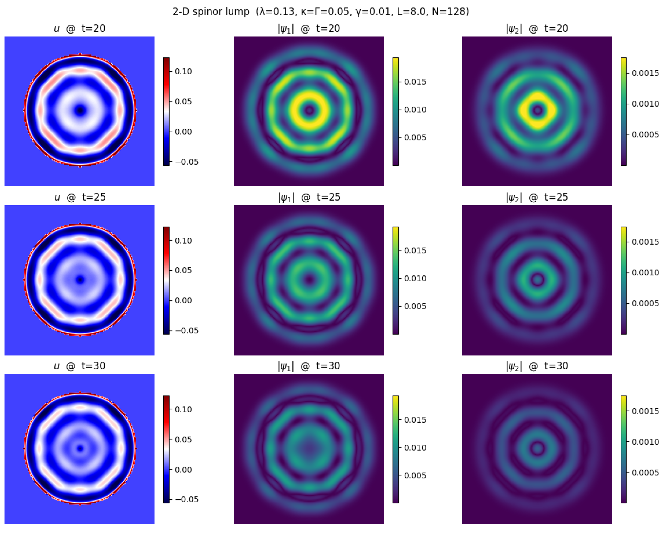
Figure 2.
Shrodinger undamped.
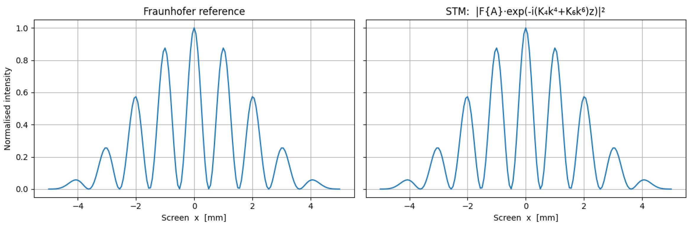
Figure 3.
Shrodinger damped.
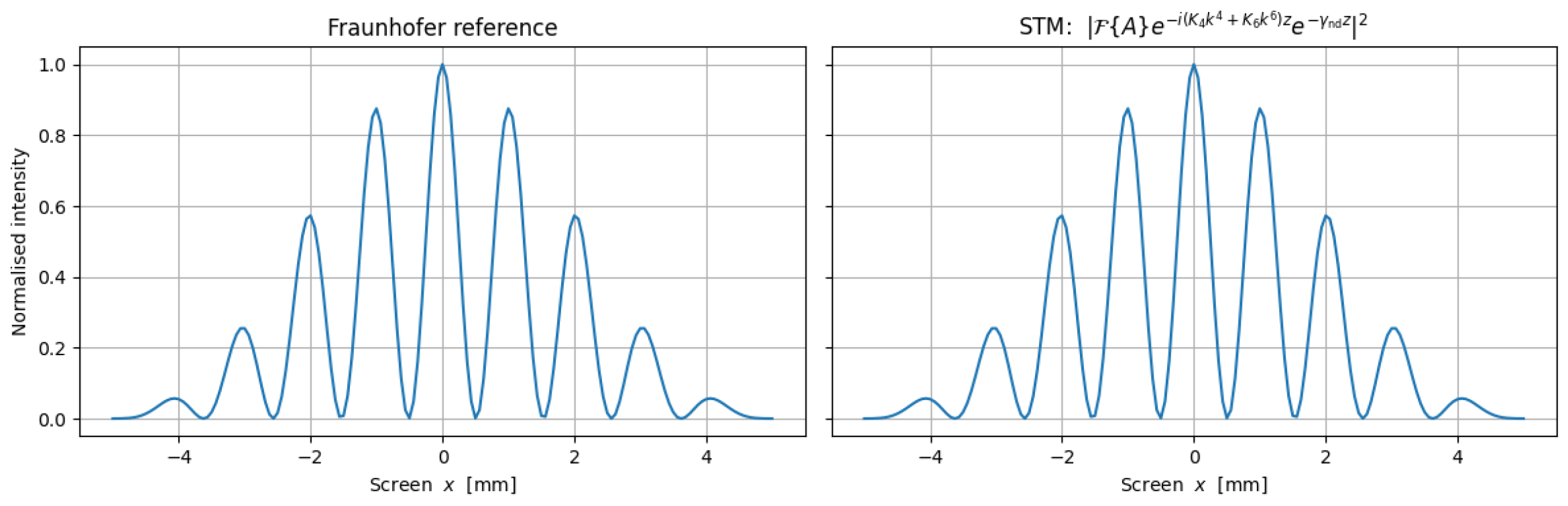
Figure 4.
Measurement.
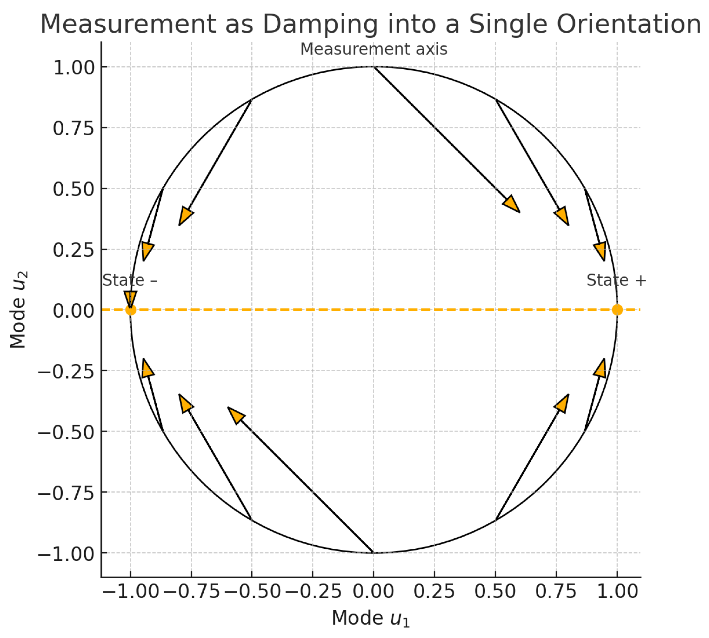
Figure 5.
STM vs PDG.
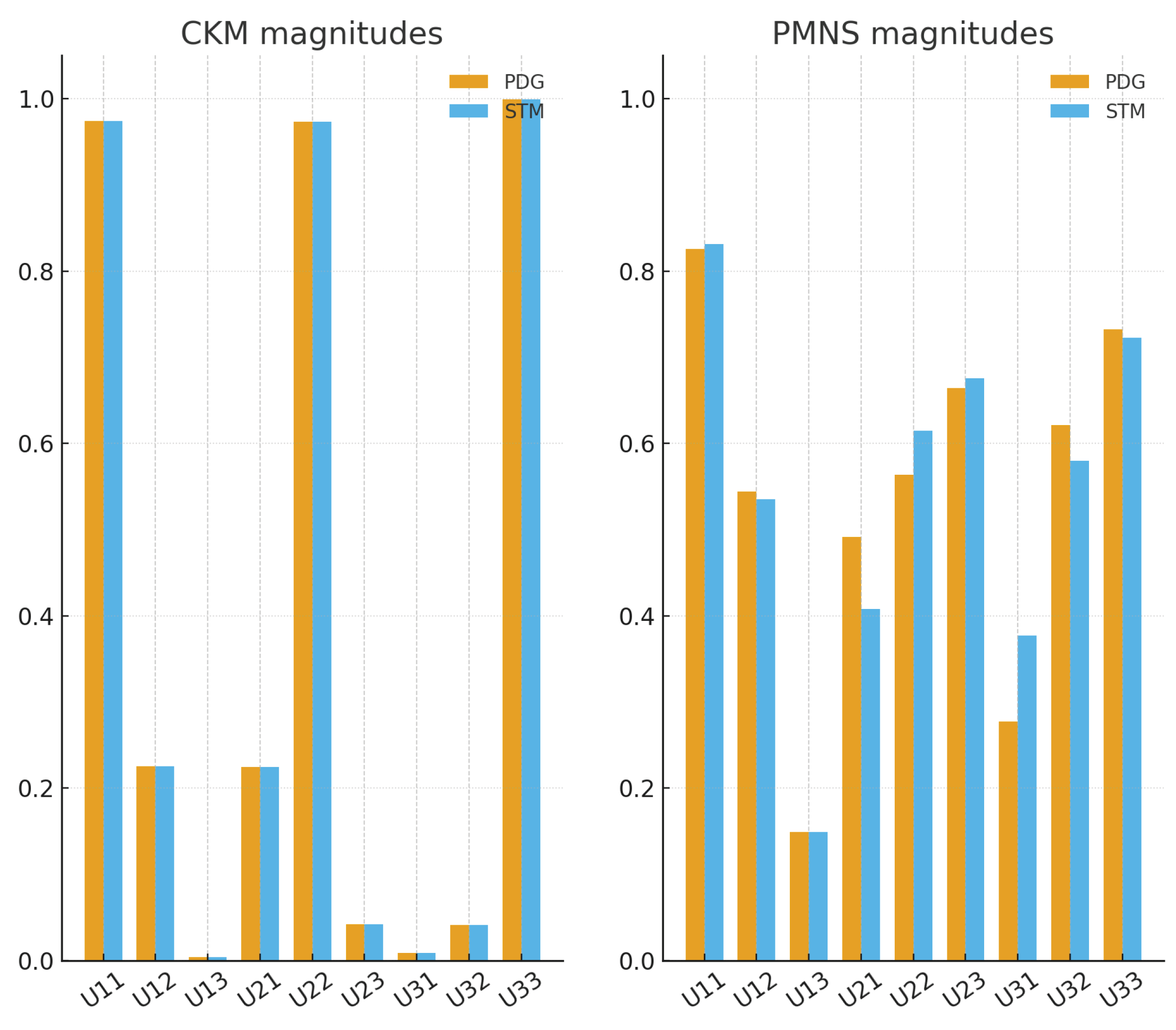
Disclaimer/Publisher’s Note: The statements, opinions and data contained in all publications are solely those of the individual author(s) and contributor(s) and not of MDPI and/or the editor(s). MDPI and/or the editor(s) disclaim responsibility for any injury to people or property resulting from any ideas, methods, instructions or products referred to in the content. |
© 2025 by the authors. Licensee MDPI, Basel, Switzerland. This article is an open access article distributed under the terms and conditions of the Creative Commons Attribution (CC BY) license (http://creativecommons.org/licenses/by/4.0/).
Copyright: This open access article is published under a Creative Commons CC BY 4.0 license, which permit the free download, distribution, and reuse, provided that the author and preprint are cited in any reuse.


