
Submitted:
06 March 2025
Posted:
07 March 2025
You are already at the latest version
Abstract
Quantum cryptography protocols offering unconditional protection open great rout to full information security in quantum era. Yet, implementing these protocols using the existing fiber networks remains challenging due to high signal losses reducing the efficiency of these protocols to zero. The recently proposed Quantum-protected Control-based Key Distribution (QCKD) addresses this issue by physically controlling interceptable losses and ensuring that leaked quantum states remain non-orthogonal. Here, we present the first in-field development and demonstration of the QCKD over an urban fiber link characterized by substantial losses. Using information-theoretic considerations, we configure the system ensuring security and investigate the interplay between line losses and secret key rates. Our results backed by the statistical analysis of the secret key, confirm QCKD’s robustness under real-world conditions, and establish it as a practical solution for quantum-safe communications over existing fiber infrastructures.
Keywords:
quantum cryptography
; quantum communication
; quantum-protected control-based key distribution
; QCKD
; loss control
; urban fiber link
; optical time-domain reflectometry
; OTDR
; quantum networks
; scalability of quantum protocols
; non-orthogonal quantum states
1. Introduction
With the rise of quantum computing, the widely used cryptographic algorithms relying on the computational complexity of certain mathematical problems—such as the RSA [1], ECC [2], and DSA [3]—face a significant threat. Namely, a sufficiently powerful quantum computer running Shor’s algorithm [4] promises to overcome these complicated mathematical problems in a short amount of time and, thus, to break the protocols’ security. Remarkably, the advances in quantum technologies offer a security–protecting counter measure: quantum cryptographic methods based on fundamental quantum properties, rather than on computational complexities [5,6,7,8,9,10,11,12,13,14,15,16,17,18] promise to guarantee secure communications. The central point of novel communication methods is quantum key distribution (QKD) [5,6,7,8,9,10,11], by which two users, commonly referred to as Alice and Bob, establish a shared random secret key through the exchange by quantum states. When used with symmetric encryption, this key guarantees full security even against the attacks with quantum computers.
Conceptually, the security of the QKD against the intrusions is based on the ability of the communicating users to detect the presence of an eavesdropper, Eve, using the fundamental laws of quantum mechanics. The eavesdropper disturbs the quantum states distributed between users in the process of their communications and, therefore, introduces measurable anomalies in the process, such as an increased bit error rate or loss of entanglement. By detecting and evaluating these anomalies in a way specific to each QKD protocol, the legitimate users determine the extent of the information breach. This allows them to take measures protecting secure key, so that none of transmitted bits becomes known to Eve.
However, when implementing these protocols in existing fiber-optic infrastructure, relying on such control mechanisms becomes problematic, as the telecommunication fiber lines have a high level of losses. Quantum signals, which usually consist of only a few photons, degrade rapidly in these lossy environments, making it not possible to rely on the state disturbances as on a direct indicator of eavesdropping. Even if the users manage to discover Eve’s presence, attributing to her all the channel losses, this will provide them little or even practically no informational advantage and, therefore, very limited achievable secret key rates.
To address these issues, recent works [19,20,21] introduced the concept of physical loss control in optical quantum communication. In this approach, users send high-intensity probe signals and analyze the transmitted and reflected components, which enables them to distinguish between localized losses exploitable by Eve and the naturally occurring, uniformly distributed scattering losses on quenched disorder that remain unusable for eavesdropping due to thermodynamic constraints [19]. By precisely determining the fraction of light which an eavesdropper could intercept, users precisely estimate Eve’s potential information gain and apply the optimal postprocessing techniques to the distributed bits to ensure key rates guaranteeing high-secrecy.
Physical loss control is a central component of the Quantum-protected Control-based Key Distribution (QCKD) [19], a prepare-and-measure protocol that encodes bits into the low-intensity coherent quantum states, and . Because these states are substantially non-orthogonal (), neither the legitimate receiver (Bob) nor an eavesdropper (Eve) can reliably distinguish them. To simplify the explanation of the QCKD, users measure the fraction of the stolen signal and verify that Eve, receiving and , cannot distinguish them better than Bob can distinguish the states he receives. Once users accurately determine their informational advantage over Eve, they postprocess their respective bit strings to produce a secure secret key about which Eve knows nothing (we note that in reality, even if Eve is better in distinguishing bits than Bob, users may still have an informational edge on account of postselection).
The QCKD has already been experimentally implemented over a 1,707 km optical fiber line in a controlled laboratory environment [22]. In this paper, we advance to the first real-world implementation of the protocol over a 4 km lossy urban fiber link within an operational fiber network. Unlike the fiber line in Ref. [22], where sections are joined through low-loss splices, the transmission line in our experiment includes multiple physical connectors that introduce significant losses, which represents the real-world fiber network conditions. We report the results of the physical loss control and the corresponding impact on key distribution rates, further verifying the quality of the resulting keys through comprehensive statistical analysis. Furthermore, we detail the physical-informational considerations defining the choice of both signal states and postprocessing parameters in our experimental setup, which itself represents a significant enhancement over the configuration in Ref. [22].
2. Protocol Description
Conceptually, the realized protocol is equivalent to that presented in Ref. [22] and follows the logic outlined in Ref. [19]. It is assumed that the users are connected via a quantum channel (optical fiber) and an authenticated classical communication channel. The procedure can be summarized as follows:
Scheme Adjustment
OTDR— Alice and Bob carry out Optical Time-Domain Reflectometry (OTDR) to identify local leakages that could be exploited by Eve and to measure the natural, homogeneous scattering losses which are considered non-interceptible [19]. Once this baseline is established, subsequent additional losses, determined at the later stage, will be attributed to Eve. The resulting reflectogram is shared over the classical channel. For details, see Section 7.1 in Methods.
Auto-tuning procedure— Alice transmits to Bob a series of phase-randomized pulses encoding a bit sequence (via their intensities), while the same bit sequence is sent over the classical channel. Bob’s detector produces a sequence of voltages, which he compares against the known bit sequence from Alice. Based on this comparison, Bob and Alice set the postselection parameters to optimize the trade-off between bit error ratio (BER) and bit loss ratio (BLR) (see Section 4).
Transmission & Control
Transmittometry— For the purpose of the loss control, Alice sends a sinusoidal signal through the quantum channel for loss estimation. The signal is modulated at a high frequency to suppress noise at Bob’s detection stage.
Quantum information transmission— Alice transmits a sequence of low-intensity pulses (633,600 pulses in one transmission). Each 33rd pulse serves as a synchronization marker. The 32 phase-randomized pulses between two consecutive synchronization pulses encode informational bits. Informational pulses are two times weaker than synchronization pulses.
Measurements— Bob measures all received signals. By analyzing the known baseline losses with the measured amplitude of the transmittometry signal, Bob estimates the exploitable leaked fraction photons of the bit-encoding signals. This estimate is sent to Alice over the classical channel. In turn, the synchronization pulses identify the start positions of each bit series, ensuring Bob that he has obtained the full series.
Postprocessing
Postselection— Bob reports to Alice via the classical channel the positions of inconclusive measurement outcomes as determined by the agreed postselection criteria. Then both parties remove these bits from their respective bit strings.
Error correction— Disclosing a small selection of bits through the classical channel, the users estimate the BER. If the error is above a certain level, see Section 4 for details, the users apply the advantage distillation procedure[23]. Once the effective BER is sufficiently reduced, low-density parity-check (LDPC) code correction is employed to remove the remaining errors. The protocol verifies that the collision probability remains below .
Privacy amplification— To ensure that Eve does not know any bits from the final key, privacy amplification is performed [24]. Knowing the observed channel losses and the amount of information revealed during error correction, the users evaluate the amount of information leaked to Eve. If the leaked information exceeds the users’ own shared information, they discard the entire bit sequence from that round. Otherwise, they apply a suitable hashing technique to compress the sequence into a shorter key, about which Eve holds no information. The compression factor is determined by the evaluated leaked information. The resulting key is added to the key storage.
The protocol leverages the non-orthogonality of bit-encoding states, implemented as phase-randomized low-intensity coherent states with different mean photon numbers. With that, the optimal strategy for both Bob and Eve to measure the transmitted bits is photon-number detection. However, because photon-number fluctuations scale as relative to the mean photon number N, there is a fundamental limit to how well bits 0 and 1 can be distinguished. For Eve, this is more problematic, since the signals she intercepts are weaker than Bob’s—which is verified by the protocol’s loss control—and therefore exhibit larger relative fluctuations. This limitation, combined with the consequent postselection, acts as the quantum protection mechanism, guaranteeing users’ information advantage over Eve.
In our experiment, Step i is repeated once every 500 cycles of Transmission & Control stage (Steps 1–3). During these 500 cycles, any interceptable local losses are updated via transmittometry, which remains reliable over this interval (see the next section for details). Step ii is executed every 20 cycles, at which point the postselection parameters are adjusted to optimize the precision of bit identification. Postprocessing (Steps 4–5) can, in turn, be applied to the raw bit sequence after the end of the active Transmisson & Control phase.
The advantage distillation used in Step 5 effectively amplifies the correlation between Alice’s and Bob’s bit sequences at the price of discarding part of the bits. In this procedure the users split their raw bit strings into blocks of length M. For each block a, Alice announces a pair of a and its inversion . If the corresponding Bob’s block matches with either-one, a now represents a “distilled” 0 bit, and “distilled” 1 bit. Otherwise, the corresponding block is discarded. As a result, the effective BER becomes , where is the BER before the distillation.
We note that the protocol’s security relies on additional assumptions regarding the used equipment, which makes it device-dependent. For more details on these assumptions and a comprehensive security analysis, we refer the reader to Ref. [19].
3. Experimental Setup
The experimental setup of the implemented QCKD is depicted in Figure 1. In Alice’s module, the laser-generated light undergoes phase randomization via a phase modulator (PM), which is driven by a random signal generator (RSG). The RSG relies on the avalanche breakdown mechanism, as detailed in Refs. [25,26]. The phase randomization [27,28,29,30] mitigates the potential of the eavesdropping attacks [31], while preserving the statistical distribution of Bob’s measurement results.
Following phase randomization, the light passes through an amplitude modulator (AM), which shapes it into optical signals—namely bit-carrying pulses, synchronization pulses and sinusoidal transmittometry signal. The AM is based on a Mach–Zehnder-type interferometer embedded in a lithium niobate crystal; applying a voltage across radio-frequency (RF) electrodes controls the optical path length. The AM’s operation is managed by a field-programmable gate array (FPGA) interfaced with a computer that hosts a quantum random number generator (QRNG). Specifically, the FPGA produces 2.5 ns- and 20 ns-long voltage pulses for bit-encoding and synchronization, respectively. These pulses are fine-tuned in amplitude by an additional electrical circuit—notated in the scheme as the bit-forming device (BFD)—before being amplified and applied to the AM’s RF ports.
A separate direct-current (DC) port on the AM is employed to stabilize the bias point and compensate for unwanted phase drifts caused by thermal fluctuations and inhomogeneities, photorefractive effects, and electrostatic charge accumulation, see Ref. [32]. This stabilization is achieved via a dedicated bias stabilizer, which provides an offset voltage determined from a power-level feedback loop, using a monitoring detector integrated into a bias control device.
Alice’s optical signals shaped by the AM are transmitted to Bob through the 4-km-long urban G.652.D single-mode optical fiber link, see Figure 1. Upon reaching Bob’s module, the incoming light first passes through a 50 GHz passband filter, is then amplified by a variable erbium-doped fiber amplifier (EDFA), and subsequently traverses a narrow-band optical filter with an 8.5 GHz bandwidth. The latter filter, employing the FBG [33], suppresses the amplified spontaneous emission (ASE) generated by the EDFA. Because the FBG is highly sensitive to temperature changes, we use a custom thermostat to maintain the filter within its specified bandwidth. The filtered optical signal is then detected by a photodetector converting it into a voltage, which is then digitized by an analog-to-digital converter (ADC), and finally processed by Bob’s computer.
The optical time-domain reflectometer is connected to the fiber line via an optical switch, as illustrated in Figure 1. In short, the OTDR involves sending a short and intense probing pulse down the line and monitoring the backscattered signal. By analyzing both the power of the returned light and its time of flight, one can determine the magnitude and precise locations of potential leakages (for more details see Ref. [19,34]).
Figure 2 presents the reflectogram obtained for the urban fiber link under study. Local losses are primarily attributed to connectors and splices. The feature highlighted in blue corresponds to the optical switch through which the reflectometer is connected on Bob’s side, while the events highlighted in pink are caused by the connectors on Alice’s side. Since these three connection points are located within controlled users’ environments, we assume that Eve cannot exploit the associated losses. From the trace in Figure 2, we estimate the total proportion of local losses intercepted by the adversary, , to be which corresponds to dB. The precision of the OTDR is dB. The utilized computational loss determination technique, which particularly implies identifying the start and end points of each local loss feature, is detailed in Section 7.1.
While the OTDR provides a detailed loss map every 500 sendings of bits (Steps 1–3 of the protocol), real-time loss monitoring is carried out via transmittometry. In this procedure, a sinusoidally modulated signal at frequency 25 MHz with duration 5 ms and power 200 nW is sent once per sending of bits. By comparing the spectral power at the modulation frequency at both the input (Alice’s side) and the output (Bob’s side), the users determine the total loss in the line. From the OTDR reflectogram, they already know the natural losses; subtracting these yields the interceptable loss . Modulating the signal helps mitigate noise. As detailed in Methods, transmittometry measurements remain accurate as long as system’s parameters, namely EDFA’s amplification coefficient, remain calibrated. Therefore, before the impact of parameters’ drift becomes comparable to the intrinsic power measurement uncertainty, the users must perform a new OTDR measurement and recalibrate transmittometry.
4. System Configuration
In this section, we explain the particular selection of these parameters in our setup based on how signal and postprocessing parameters affect the secret key generation rate. In the case where postselection yields the outcomes 0 and 1 with equal probability and postprocessing includes advantage distillation with block length M, the secret key rate (in bits per channel use) is given by the Devetak–Winter formula [35] as follows:
where is the binary entropy function, and are the BERs before and after advantage distillation, respectively, is the efficiency factor for the employed error-correcting code, and is mutual information between Alice and Eve after postselection and advantage distillation. In its explicit form, provided in Section 7.2 in Methods, depends on , the intensities and of the signals encoding bits 0 and 1, respectively, and the choice of M. A detailed derivation of Eq. (1) can be found in Ref. [22].
The resulting analytical expression defines the set of system parameters—namely, the intensities and , the advantage distillation block size M, and the privacy amplification compression factor—that ensure a positive secret key rate at the specified value of . In principle, all of these parameters could be adaptively selected to maximize R each time users update the value of . In the present experiment, however, we adopt a simpler strategy: we only adapt the privacy amplification compression factor when changes, while keeping the other parameters fixed throughout all protocol runs.
The signal intensities and are selected to ensure that, for of around 20 % (as observed in the experiment), the secret key rate R from Eq. (1) remains positive, which corresponds to an informational advantage over Eve. Specifically, using Eq. (1), for various and we calculate the critical value of that sets . Then, for the experiment, we choose and such that the corresponding critical is above 20 % with about 10 % overhead. If, at any point during the experiment, the measured exceeds the critical value, the corresponding bits are discarded. Conversely, if is below the critical value, the users evaluate the corresponding amount of Eve’s information, apply appropriate privacy amplification, and generate the corresponding amount of secret key as prescribed by Eq. (1).
Figure 3 shows the calculated critical as a function of and for the effective BER . Panel (a) covers a wider range of intensities, while panel (b) focuses on a narrower range with the critical near the experimentally observed with some overhead. The marked point in Figure 3(b) corresponds to our experimental choice of intensities photons and photons. The particular choice of is motivated by the constraints of the LDPC-based error correction realization utilized in our scheme, which is optimized for BER below 5 %. Under the experimental conditions—with the chosen and and using empirically picked postselection parameters—we observe a raw BER of . After advantage distillation with the block size , the effective BER close to 5 %, meeting the requirements of the LDPC procedure. An extended table of intensities and critical is provided in Section 7.3 in Methods.
Although in the experiment we perform advantage distillation with , choosing other value of M can also yield positive secret key rate R. The numerically calculated R as a function of for is plotted in Figure 4. Within the highlighted experimentally observed range of , ensures the best secret key rates, while and allow for less optimal results. Other choices of , not represented in the plot result in substantially worse R. Note that without advantage distillation () the amount of information disclosed with error correction is so high, that the users lose informational edge over Eve, and .
5. Results
Figure 5 shows the experimentally observed dynamics of the interceptable leakage and secret key rate R. The horizontal axis corresponds to the number of conducted cycles of Transmission & Control (Steps 1–3 of the protocol), N. Within the time interval reflected in Figure 5, the measured varies between 19 % and 22 %, while R correspondingly changes within the range from and bits per channel use. The average R is bits per channel use which translates into 490 bit/s given that the average rate at which Alice transmits bits is 614 kbit/s.
Due to the intrinsic transmittometry error, on a short scale of N, the measured value of fluctuates by . With that, the selected measurement time interval in Figure 5 is such that any systematic error due to the system’s detuning (see Section 7.1 in Methods for details) remains below the same threshold of . Both of these measurement uncertainties are accounted for during the Postprocessing phase by taking that Eve holds for every measured .
Note that the secret key rate R in Figure 5 appears constant over intervals of to 10 Transmission & Control cycles. This is because the used error correction implementation required users to have a minimum number of raw bits, which cannot be harvested within a single cycle. Consequently, secret keys are generated only after sufficient bits have been accumulated, typically over to 10 cycles, depending on the error rate. Although each cycle has its own measured , in privacy amplification of the combined data, we apply the maximum from the measured values to the entire accumulated sequence. Within each interval, the plotted R represents an average over those cycles, which looks like a constant.
The statistical quality of the generated key is demonstrated in Figure 6, where we plot (a) the mean and (b) the variance of the consecutive n bits of the key as function of n, and compare these values to those expected from an ideal equiprobable binomial distribution. Analyzing statistics within consecutive blocks of length n is beneficial since it fully reflects the quality of the key in respect to the potential noises of different frequencies. We find that the mean deviates from the ideal on average by a negligibly small value, in the order of one thousandth’s of a percent. Similarly, the variance discrepancy remains within two standard deviations (see Section 7.4 in Methods for details on their calculation) from the ideal . In this scope, it is important to note that these properties of the key lie within statistical error caused by a finite length of the samples across the full range of n observed in the experiment. In other words, the fidelity of the statistical model applied to experimental data is high, though it decreases slightly for a small fraction of block lengths. Additionally, in Figure 6 (c) we show the fluctuations of the mean along with its autocorrelation function for a fixed block length (). In support of this, the key passes the full suite of NIST statistical tests, as summarized in Table 1. Taken together, these results affirm the statistical quality of the secret key and absence of correlations.
6. Discussion
In this study, we have experimentally realized QCKD using the real-world fiber infrastructure. The security of the protocol is ensured by the appropriate system configuration based on the information theoretic analysis. The presented experimental results show that the precision of the loss control and the dynamics of losses within a real-life telecommunication line allow for the secret key rate of 490 bit/s on average. With that, the presented statistical analysis of the resulting key underscores its high quality for secure communication. Our results show the practical way of deploying quantum-resistant communications through adopting the existing fiber infrastructure.
The study shows that QCKD remains secure even in the presence of high-loss connectors within the transmission line. Thus, we expect that the system would tolerate the introduction of additional users through imperfect optical switches, as proposed in Ref. [22]. To this end, we further plan to demonstrate a multi-node implementation of the QCKD within a single telecommunication network. We also expect that several additional enhancements—such as high-frequency OTDR monitoring, expanding the bit ciphering bandwidth at Alice’s side, and improving the detection apparatus—will further increase the secret bit rate and overall efficiency of the protocol. These developments will be addressed in our subsequent publications.
7. Methods
7.1. OTDR and Transmittometry
The following is the method that we use to identify points of local losses and their magnitude from a reflectogram, namely in Figure 2. First, the raw trace is smoothed using a moving average filter. Then, we calculate the gradient of this smoothed signal at every point. In regions exhibiting only natural losses, the gradient remains within predefined threshold values; any gradient excursion beyond these thresholds is taken as evidence of a local loss event. The magnitude of the local loss is obtained from the power difference between the start and end points of the identified local feature.
Applying this method to our 4 km fiber link, we measure a total natural loss of approximately 0.635 dB (13.6 %), in agreement with the expected Rayleigh scattering for this distance. At the beginning of the link, the first peak in the trace corresponds to the light reflection on the input connector, followed by three localized losses measured at 0.543 dB (11.8 %), 0.010 dB (0.2 %), and 0.439 dB (9.6 %), respectively. At the opposite end, the final peak corresponds to the reflection on the isolator, while two additional connectors within Alice’s trusted zone give loss values of 0.708 dB (15.0 %) and 0.398 dB (8.8 %). Consequently, the total event loss—determined as the sum of all event losses outside Alice’s and Bob’s laboratories—amounts to 0.993 dB (20.4 %).
During transmittometry, Alice sends a signal with power nW, modulated at a frequency 25 MHz. Bob then receives this signal, performs a Fourier transform, and obtains its output spectral power . He communicates back to Alice through a classical channel. Because
where G is the amplification factor of Bob’s EDFA and is the loss on the connectors within Alice’s and Bob’s laboratories (corresponding to the blue and red regions in Figure 2), the users calculate using
Our OTDR measurements indicate that, over a 12-hour period, and remain constant within 0.2 %, while is preserved through the control of Alice’s laser. Detector’s dark noise and the amplified spontaneous emission (ASE) from the EDFA may contribute to the uncertainty in the transmittometry measurements. To eliminate potential systematic errors arising from possible drifts in G, or , we perform OTDR every two hours and recalibrate the parameters in Eq. (3). In principle, OTDR can be carried out more frequently if needed.
7.2. Eve’s Information
Let us derive an analytical expression for the mutual information between Alice and Eve after postselection and advantage distillation, , in the scenario where Eve intercepts a fraction of the signal intensity, and Alice and Bob apply advantage distillation with a block size M.
To encode the bit , Alice prepares phase-randomized coherent state with intensity , which density matrix is given by
Diverting the fraction of the signal, Eve obtains the corresponding state
Note that the postselection procedure employed by Alice and Bob does not change the overall probability distribution of the bits, and—as long as the transmission line contains no elements (e.g., optical amplifiers) that introduce additional correlations between Bob’s and Eve’s states—the state remains independent of postselection [19].
In the advantage distillation step, Alice groups her bits into blocks of length M and for each block publicly discloses, that its value is either or its bitwise complement . Therefore, Eve’s task is to distinguish two equiprobable product states: and . To quantify the maximum information that Eve can extract, we apply the Holevo theorem [36] and maximize over all pairs of opposing blocks. Thus, Eve’s information is expressed as
where is the von Neumann entropy. By substituting Eq. (5) into Eq. (6), one obtains an explicit form of Eve’s information. This expression is then incorporated into Eq. (1) to calculate the secret key rate.
7.3. Critical Leakage Data
By picking a particular pair of intensities for bit-encoding pulses, Alice and Bob determine the tolerance for an observed leakage value . Figure 7 shows an extended table of critical value as a function of signal intensities. The critical leakage achieves its maximum when the intensity values are close to each other.
7.4. Statistical Analysis
On par with the NIST Statistical Test, the results of which are presented in Table 1, we perform additional analysis of the central moments of the key distribution, that may provide better understanding of the key’s quality. Ideally, the secret bit sequence must follow the equiprobable Bernoulli distribution. To check this, we divide this array of bits into consecutive blocks of length n, and for each of these blocks, we calculate the sum of its bit values, producing a random variable . This division would result in a random sample of size , in which are taken from a population following binomial distribution with . Therefore, analyzing the central moments would allow us to know how far the initial distribution is from the ideal theoretical model. More precisely, if the central moment of the sample is too far from its theoretical prediction, the fidelity of the model would be questioned for this particular n.
This approach allows us to identify the frequency of the noise, should it worsen the quality of the key. In this way, by increasing the length of the blocks n, we shift our focus from higher to lower frequency noise, as small blocks fail to capture low frequency effects. For this reason, we test the final key on a wide range of n, tracing the deviation from the theoretical model.
The results for the first two central moments are presented in Figure 6 (a, b). The error bars in these plots reflect the finiteness of the sample size , and in our case can be easily found only for the first two moments. We first note that the binomial distribution tends to the Gaussian distribution in the limit . Therefore, our objective reduces to determining the variance of the random sample , where each is drawn from a Gaussian population with variance . For such an unbiased sample variance, it is known that has a chi-squared distribution with degrees of freedom. In our case, .
Therefore, we can determine that
where is the variance of the sample data. This result allows us to plot a confidence intervals in Figure 6 (b).
A similar result can be obtained for the sampling distribution of the sample mean. This result is called the central limit theorem, which in our case leads to the following result:
This analysis is shown in Figure 6 (a). Finally, in Figure 6 (c) we show the dynamics of the parameter p, fitting the experimental data to the theoretical model described above for a fixed value of n. A small deviation of the estimated value of p from the target value and small values of its autocorrelation confirm the high quality of the final key.
According to these results, the final key is well described by the model. In particular, the bits in the final key can be represented as random variables following a Bernoulli distribution with a parameter , within the limits of statistical precision. Consequently, we can conclude that any noise affecting the key statistics has been effectively mitigated by the postprocessing methods used.
Author Contributions
M.P. and V.V. conceptualized the work; V.St. and A.A. designed the experiment; V.St., V.Sem., D.K., and V.Z. assembled the experimental setup. V.St. and A.A. collected and processed data related to the distributed key. A.A. conducted a statistical analysis and quality assessment of the key. V.St., V.Sem., D.K., and V.Z. gathered and analyzed the OTDR experimental data. V.St. and V.Sem. wrote software; V.Sem., D.K., and V.Z. arranged hardware’s design and assembly. V.V., A.K. and V.P. developed the theory. All authors participated in writing the manuscript. All authors have read and agreed to the published version of the manuscript.
Funding
This work is supported by Terra Quantum AG.
Institutional Review Board Statement
Not applicable.
Informed Consent Statement
Not applicable.
Data Availability Statement
Additional information data may be obtained from the authors upon a request.
Acknowledgments
This work is supported by Terra Quantum AG.
Conflicts of Interest
The authors declare no conflicts of interest.
Abbreviations
The following abbreviations are used in this manuscript:
| ADC | Analog-to-digital converter |
| AM | Amplitude modulator |
| BER | Bit error ratio |
| BLR | Bit loss ratio |
| DFB | Distributed-feedback |
| DSA | Digital Signature Algorithm |
| ECC | Elliptic-curve cryptography |
| EDFA | Erbium-doped fiber amplifier |
| FBG | Fiber Bragg grating |
| FPGA | Field-programmable gate array |
| LDPC | Low-density parity-check |
| OTDR | Optical time-domain reflectometry |
| PM | Phase modulator |
| QCKD | Quantum-protected Control-based Key Distribution |
| QRNG | Quantum random number generator |
| RSG | Random signal generator |
| VOA | Variable optical attenuator |
References
- Rivest, R.L.; Shamir, A.; Adleman, L. A method for obtaining digital signatures and public-key cryptosystems. Commun. ACM 1978, 21, 120–126. [Google Scholar] [CrossRef]
- Koblitz, N. Elliptic curve cryptosystems. Mathematics of Computation 1987, 48, 203–209. [Google Scholar]
- Kravitz, D.W. Digital Signature Algorithm. US Patent No. US5231668A 1993. [Google Scholar]
- Shor, P. Algorithms for quantum computation: discrete logarithms and factoring. In Proceedings of the Proceedings 35th Annual Symposium on Foundations of Computer Science; 1994; pp. 124–134. [Google Scholar] [CrossRef]
- Bennett, C.H.; Brassard, G. Quantum cryptography: Public key distribution and coin tossing. Theoretical Computer Science 2014, 560, 7–11. [Google Scholar] [CrossRef]
- Ekert, A.K. Quantum cryptography based on Bell’s theorem. Phys. Rev. Lett. 1991, 67, 661–663. [Google Scholar]
- Bennett, C.H. Quantum cryptography using any two nonorthogonal states. Phys. Rev. Lett. 1992, 68, 3121–3124. [Google Scholar] [CrossRef]
- Bruß, D. Optimal Eavesdropping in Quantum Cryptography with Six States. Phys. Rev. Lett. 1998, 81, 3018–3021. [Google Scholar] [CrossRef]
- Pirandola, S.; Andersen, U.L.; Banchi, L.; Berta, M.; Bunandar, D.; Colbeck, R.; Englund, D.; Gehring, T.; Lupo, C.; Ottaviani, C.; et al. Advances in quantum cryptography. Advances in Optics and Photonics 2020, 12, 1012. [Google Scholar] [CrossRef]
- Gu, J.; Cao, X.Y.; Fu, Y.; He, Z.W.; Yin, Z.J.; Yin, H.L.; Chen, Z.B. Experimental measurement-device-independent type quantum key distribution with flawed and correlated sources. Science Bulletin 2022, 67, 2167–2175. [Google Scholar] [CrossRef]
- Xie, Y.M.; Lu, Y.S.; Weng, C.X.; Cao, X.Y.; Jia, Z.Y.; Bao, Y.; Wang, Y.; Fu, Y.; Yin, H.L.; Chen, Z.B. Breaking the Rate-Loss Bound of Quantum Key Distribution with Asynchronous Two-Photon Interference. PRX Quantum 2022, 3, 020315. [Google Scholar] [CrossRef]
- Hu, J.Y.; Yu, B.; Jing, M.Y.; Xiao, L.T.; Jia, S.T.; Qin, G.Q.; Long, G.L. Experimental quantum secure direct communication with single photons. Light Sci. Appl. 2016, 5, e16144. [Google Scholar] [CrossRef] [PubMed]
- Lucamarini, M.; Yuan, Z.L.; Dynes, J.F.; Shields, A.J.; All, A. Overcoming the rate–distance limit of quantum key distribution without quantum repeaters. Nature 2018, 557, 400–403. [Google Scholar] [CrossRef]
- Qi, Z.; Li, Y.; Huang, Y.; Feng, J.; Zheng, Y.; Chen, X. A 15-user quantum secure direct communication network. Light Sci. Appl. 2021, 10, 183. [Google Scholar] [CrossRef] [PubMed]
- Ma, X.; Qi, B.; Zhao, Y.; Lo, H.K. Practical decoy state for quantum key distribution. Physical Review A—Atomic, Molecular, and Optical Physics 2005, 72, 012326. [Google Scholar] [CrossRef]
- Scarani, V.; Acin, A.; Ribordy, G.; Gisin, N. Quantum Cryptography Protocols Robust against Photon Number Splitting Attacks for Weak Laser Pulse Implementations. Physical review letters 2004, 92, 057901. [Google Scholar] [CrossRef]
- Zhang, H.; Sun, Z.; Qi, R.; Yin, L.; Long, G.L.; Lu, J. Realization of quantum secure direct communication over 100 km fiber with time-bin and phase quantum states. Light Sci. Appl. 2022, 11, 83. [Google Scholar] [CrossRef]
- Long, G.L.; Pan, D.; Sheng, Y.B.; Xue, Q.; Lu, J.; Hanzo, L. An Evolutionary Pathway for the Quantum Internet Relying on Secure Classical Repeaters. IEEE Network 2022, 36, 82–88. [Google Scholar] [CrossRef]
- Kirsanov, N.S.; Pastushenko, V.A.; Kodukhov, A.D.; Yarovikov, M.V.; Sagingalieva, A.B.; Kronberg, D.A.; Pflitsch, M.; Vinokur, V.M. Forty thousand kilometers under quantum protection. Scientific Reports 2023, 13, 8756. [Google Scholar] [CrossRef]
- Smirnov, A.; Yarovikov, M.; Zhdanova, E.; Gutor, A.; Vyatkin, M. An Optical-Fiber-Based Key for Remote Authentication of Users and Optical Fiber Lines. Sensors 2023, 23, 6390. [Google Scholar] [CrossRef]
- Kodukhov, A.D.; Pastushenko, V.A.; Kirsanov, N.S.; Kronberg, D.A.; Pflitsch, M.; Vinokur, V.M. Boosting Quantum Key Distribution via the End-to-End Loss Control. Cryptography 2023, 7, 38. [Google Scholar] [CrossRef]
- Kirsanov, N.; Pastushenko, V.; Kodukhov, A.; Aliev, A.; Yarovikov, M.; Strizhak, D.; Zarubin, I.; Smirnov, A.; Pflitsch, M.; Vinokur, V. Loss Control-Based Key Distribution under Quantum Protection. Entropy 2024, 26. [Google Scholar] [CrossRef]
- Maurer, U. Secret key agreement by public discussion from common information. IEEE Transactions on Information Theory 1993, 39, 733–742. [Google Scholar] [CrossRef]
- Bennett, C.H.; Brassard, G.; Robert, J.M. Privacy Amplification by Public Discussion. SIAM Journal on Computing 1988, 17, 210–229. [Google Scholar] [CrossRef]
- McKay, K.G. Avalanche Breakdown in Silicon. Phys. Rev. 1954, 94, 877–884. [Google Scholar] [CrossRef]
- Lampert, B.; Wahby, R.S.; Leonard, S.; Levis, P.; All, A. Robust, low-cost, auditable random number generation for embedded system security. In Proceedings of the Proceedings of the 14th ACM Conference on Embedded Network Sensor Systems CD-ROM. [CrossRef]
- Mølmer, K. Optical coherence: A convenient fiction. Phys. Rev. A 1997, 55, 3195–3203. [Google Scholar] [CrossRef]
- Lütkenhaus, N. Security against individual attacks for realistic quantum key distribution. Phys. Rev. A 2000, 61, 052304. [Google Scholar] [CrossRef]
- van Enk, S.J.; Fuchs, C.A. Quantum State of an Ideal Propagating Laser Field. Phys. Rev. Lett. 2001, 88, 027902. [Google Scholar] [CrossRef]
- Zhao, Y.; Qi, B.; Lo, H.K. Experimental quantum key distribution with active phase randomization. Applied Physics Letters 2007, 90, 044106. [Google Scholar] [CrossRef]
- Preskill, J.; Lo, H. Phase randomization improves the security of quantum key distribution. arXiv preprint quant-ph/0504209.
- Sun, S.; He, M.; Xu, M.; Gao, S.; Chen, Z.; Zhang, X.; Ruan, Z.; Wu, X.; Zhou, L.; Liu, L.; et al. Bias-drift-free Mach–Zehnder modulators based on a heterogeneous silicon and lithium niobate platform. Photon. Res. 2020, 8, 1958–1963. [Google Scholar] [CrossRef]
- Hill, K.O.; Fujii, Y.; Johnson, D.C.; Kawasaki, B.S.; All, A. Photosensitivity in optical fiber waveguides: Application to reflection filter fabrication. Applied Physics Letters 1978, 32, 647–649. [Google Scholar] [CrossRef]
- Smirnov, A.; Yarovikov, M.; Zhdanova, E.; Gutor, A.; Vyatkin, M. An optical-fiber-based key for remote authentication of users and optical fiber lines. Sensors 2023, 23, 6390. [Google Scholar] [CrossRef] [PubMed]
- Devetak, I.; Winter, A. Distillation of secret key and entanglement from quantum states. Proceedings of the Royal Society A: Mathematical, Physical and engineering sciences 2005, 461, 207–235. [Google Scholar]
- Holevo, A.S. Bounds for the quantity of information transmitted by a quantum communication channel. Problems Inform. Transmission 1973, 9, 177–183. [Google Scholar]
Figure 1.
Schematics of the setup. On Alice’s side, a distributed-feedback (DFB) laser emits light at a wavelength of 1530.33 nm, with its phase randomized by a phase modulator (PM) connected to a random signal generator (RSG). The light is modulated into bit-carrying pulses, synchronization pulses, or a sinusoidal signal by an amplitude modulator (AM), which is controlled by Alice’s computational hardware. The modulated signal is attenuated by a variable optical attenuator (VOA) and passes through an isolator into a 4-km-long urban fiber link. At Bob’s side, the signal is first passed through a 50 GHz preliminary bandpass filter before entering an erbium-doped fiber amplifier (EDFA), then through a narrowband fiber Bragg grating (FBG) filter, and finally detected by a photodetector. The output from the photodetector is converted into digital data by an analog-to-digital converter (ADC) on Bob’s computer. Optical time-domain reflectometer (OTDR) is connected to the line via an optical switch on Bob’s side.
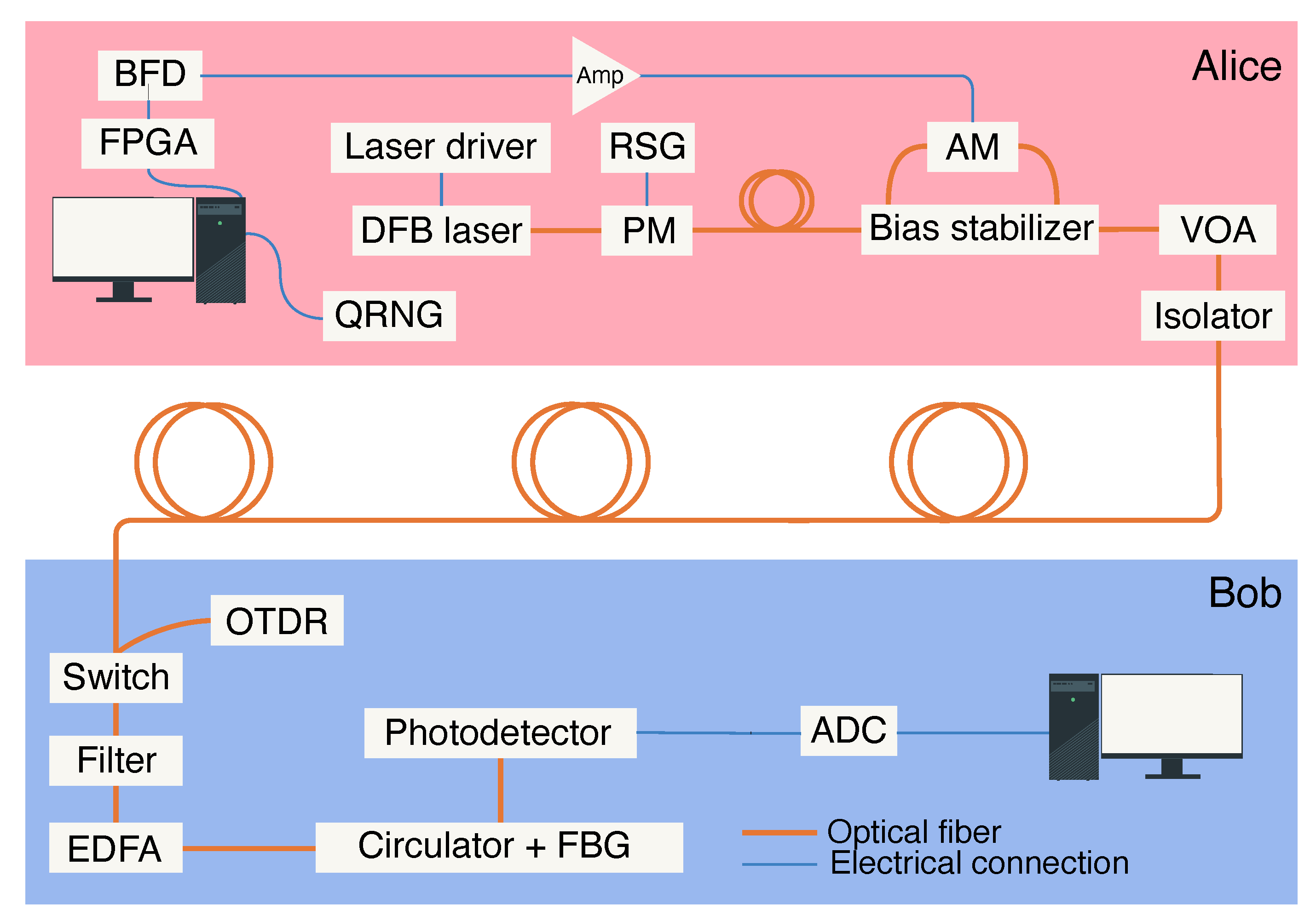
Figure 2.
OTDR trace of the transmission line. This reflectogram, plotting backscattered power as a function of distance, allows one to isolate localized leakages exploitable by Eve from the natural, uniformly distributed losses caused by Rayleigh scattering on density fluctuations in the fiber. The natural losses are responsible for the trace’s linear decay. The start and end points of the localized leaks are highlighted by the green markers. The blue and red regions of the plot lie within Bob’s and Alice’s respective controlled environments, making the respective leakages inaccessible to Eve. In total, the interceptible localized leakage amounts to 20.4 % (0.993 dB), while the natural losses account for 13.6 % (0.635 dB).
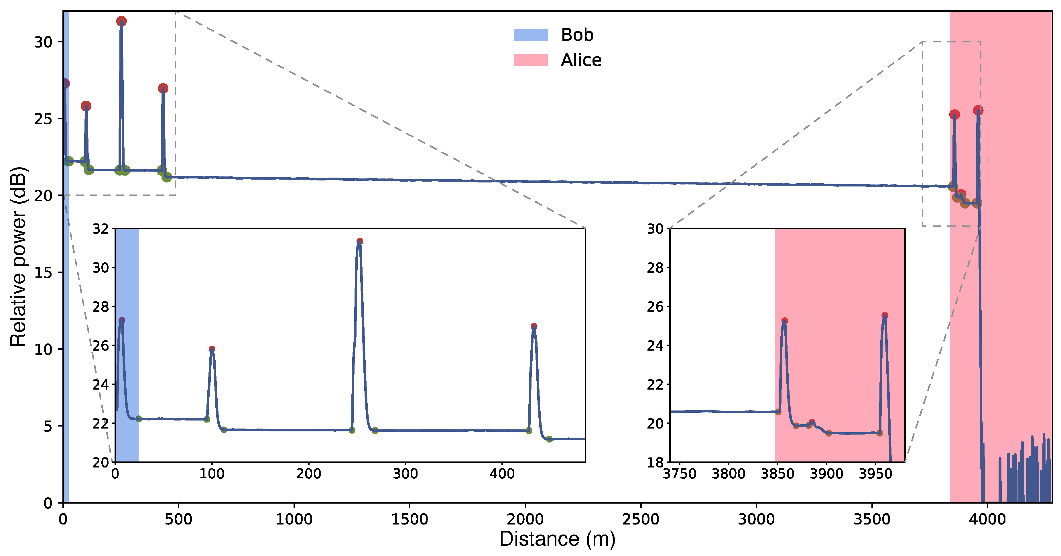
Figure 3.
Critical providing positive secret key generation rate for depicted as a function of signal intensities. Light yellow parts of the graphs correspond to the pairs of intensities for which every is acceptable, as long as the legitimate users can achieve after advantage distillation. (a) The signal intensities are sampled from sets with relatively wide boundaries: , . (b) The signal intensities are sampled from sets with more narrow boundaries: , .
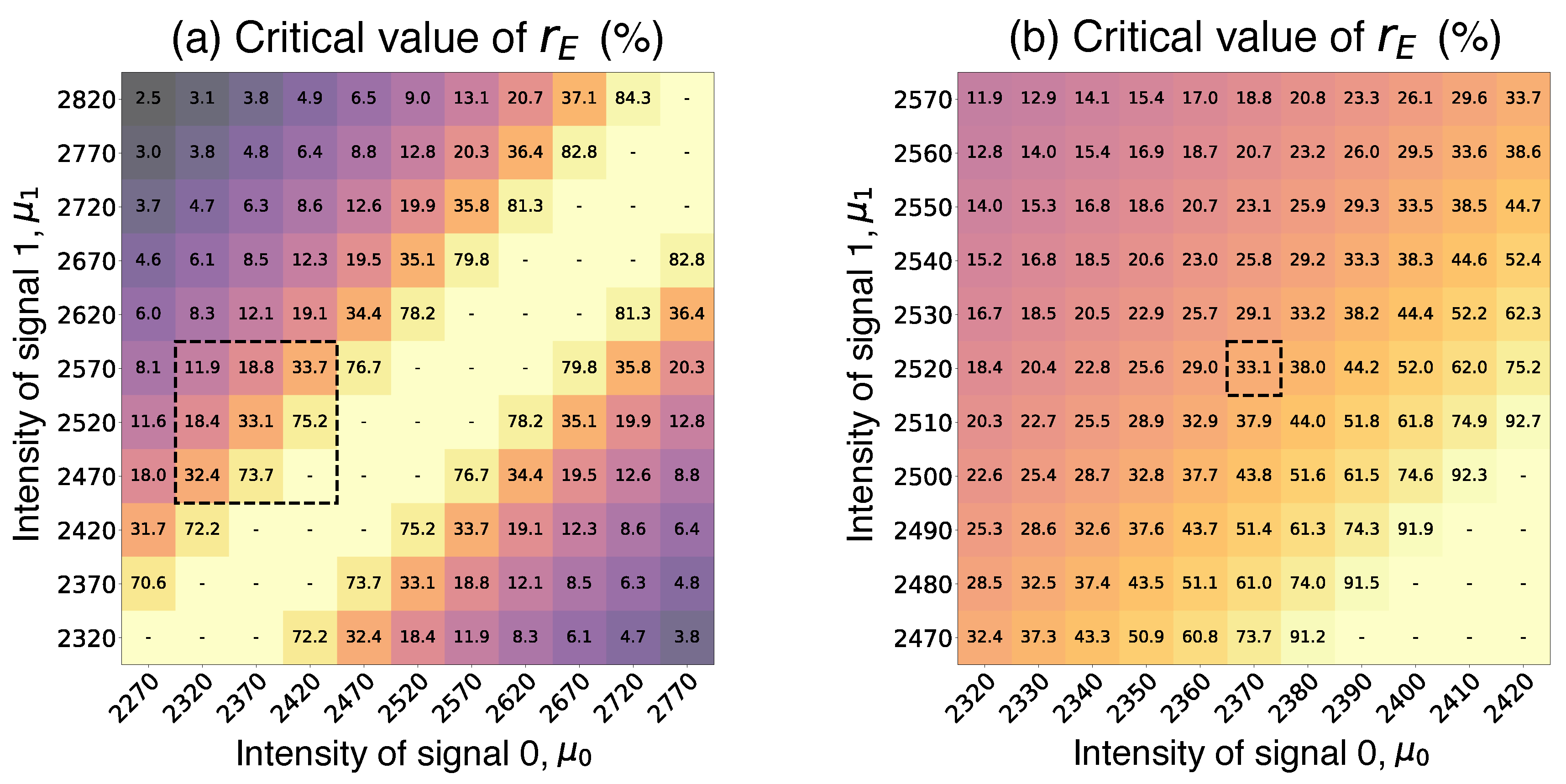
Figure 4.
Secret key rate R (in bits per channel use) as a function of interceptable leakage for different advantage distillation block lengths M. The white region indicates the range of observed in the experiment.
Figure 4.
Secret key rate R (in bits per channel use) as a function of interceptable leakage for different advantage distillation block lengths M. The white region indicates the range of observed in the experiment.
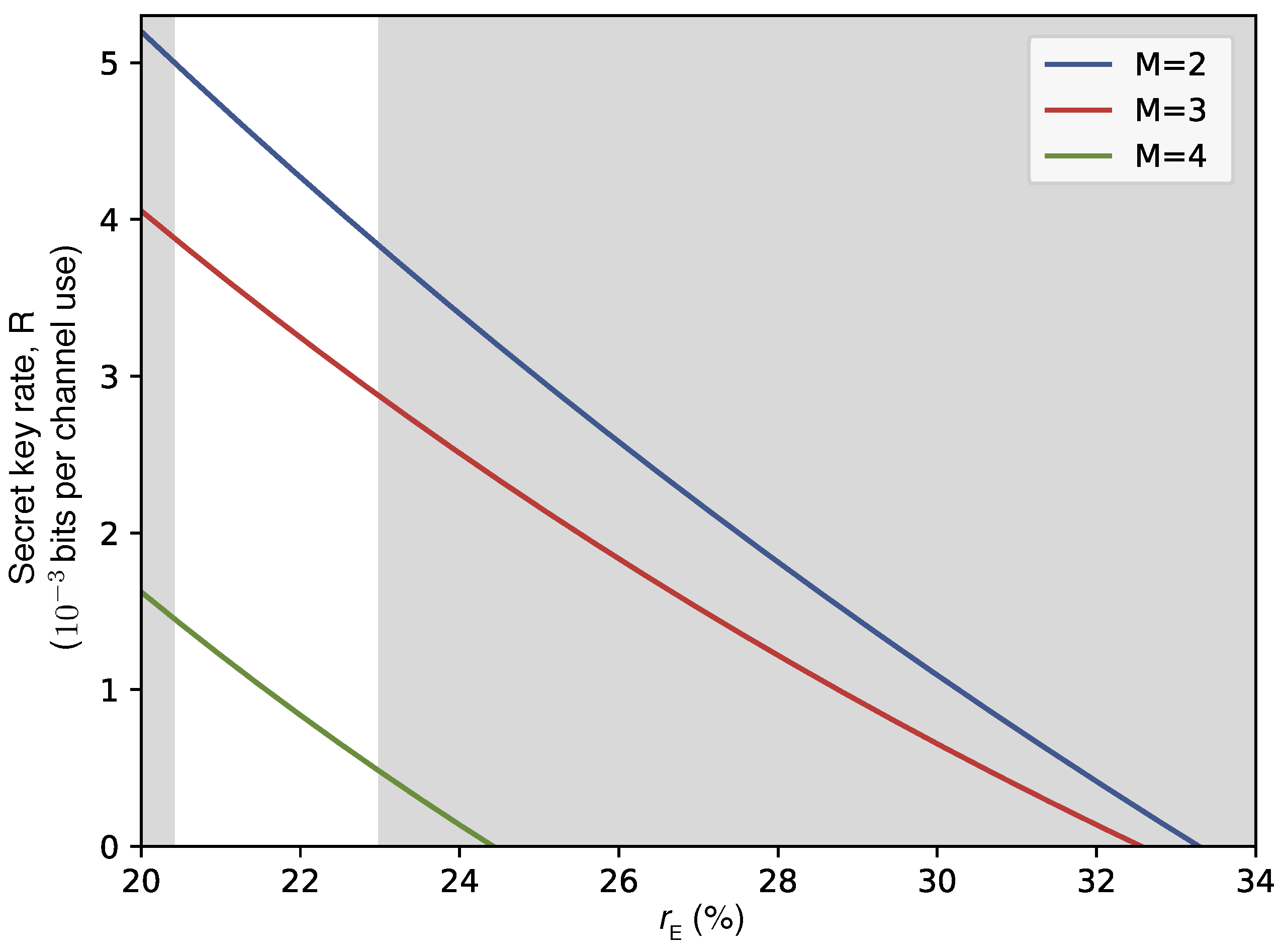
Figure 5.
Dynamics of the secret key rate and losses. The lower blue trace shows the secret key rate R (in bits per channel use) as a function of the number of Transmission & Control cycles N. The upper red trace displays the corresponding value of . Note that key postprocessing is performed after accumulating data over intervals of to 10 cycles. Consequently, the plotted R is an average computed over each interval, appearing as a constant value within that range. The dashed horizontal line indicates the global average of R.
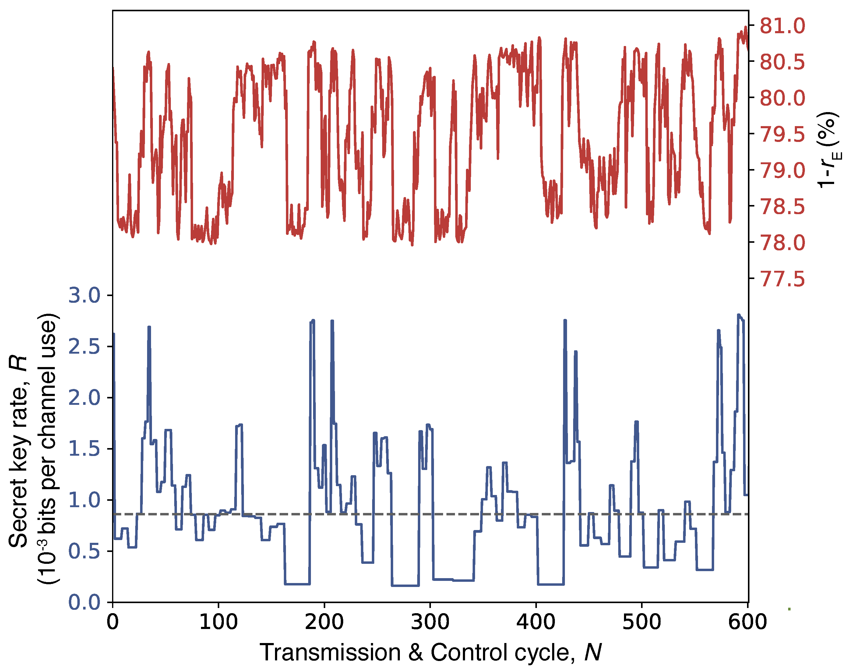
Figure 6.
Statistical analysis of the final key. The blue line represent to the final key statistic fitted to theoretical model. The mean (a) of the sum of bit values within blocks is compared to the theoretical prediction for a wide range of block lengths. Further, the variance (b) of this sum across the sample is compared to the theoretical model. Fidelity in these figures stands for the percentage of the lengths of the blocks for which experimental results fit with the experimental model within the confidence interval. The latter is represented by the error bars, and a fit to the population central moments as a function of n is depicted by a green line. Panel (c), which depicts the parameter p that provides the closest fit to the theoretical model (see Section 7.4 in Methods), shows how it changes throughout multiple Transmission & Control cycles, and its autocorrelation (black line). For this demonstration, the length of the blocks was taken as .
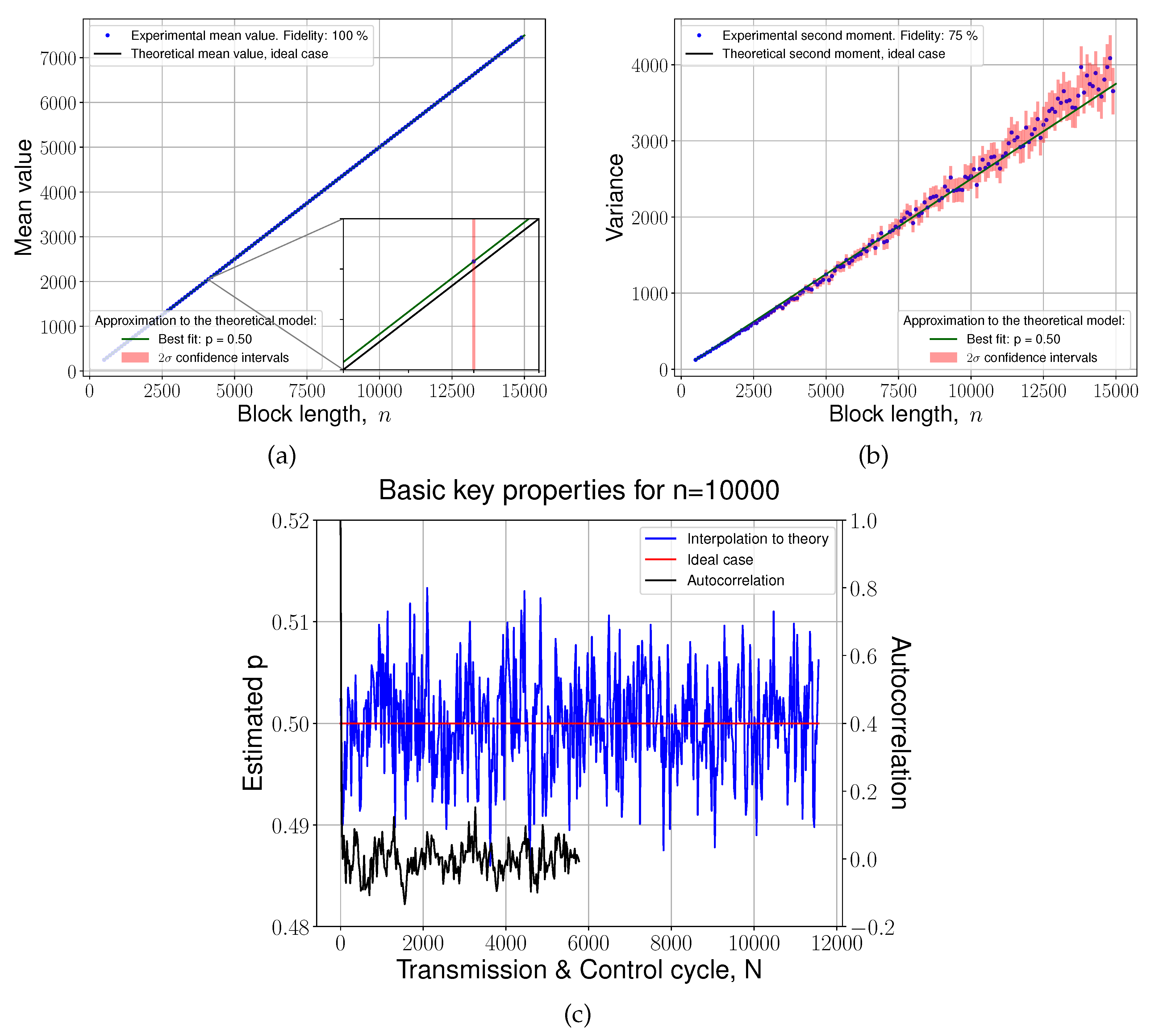
Figure 7.
Critical as a function of signal intensities and . The advantage distillation block length is . The BER value after advantage distillation does not exceed 5 %. Cells with a dash (light yellow parts) correspond to the pairs of intensities () for which every leakage value is acceptable. The signal intensities are sampled from sets with the boundaries: .
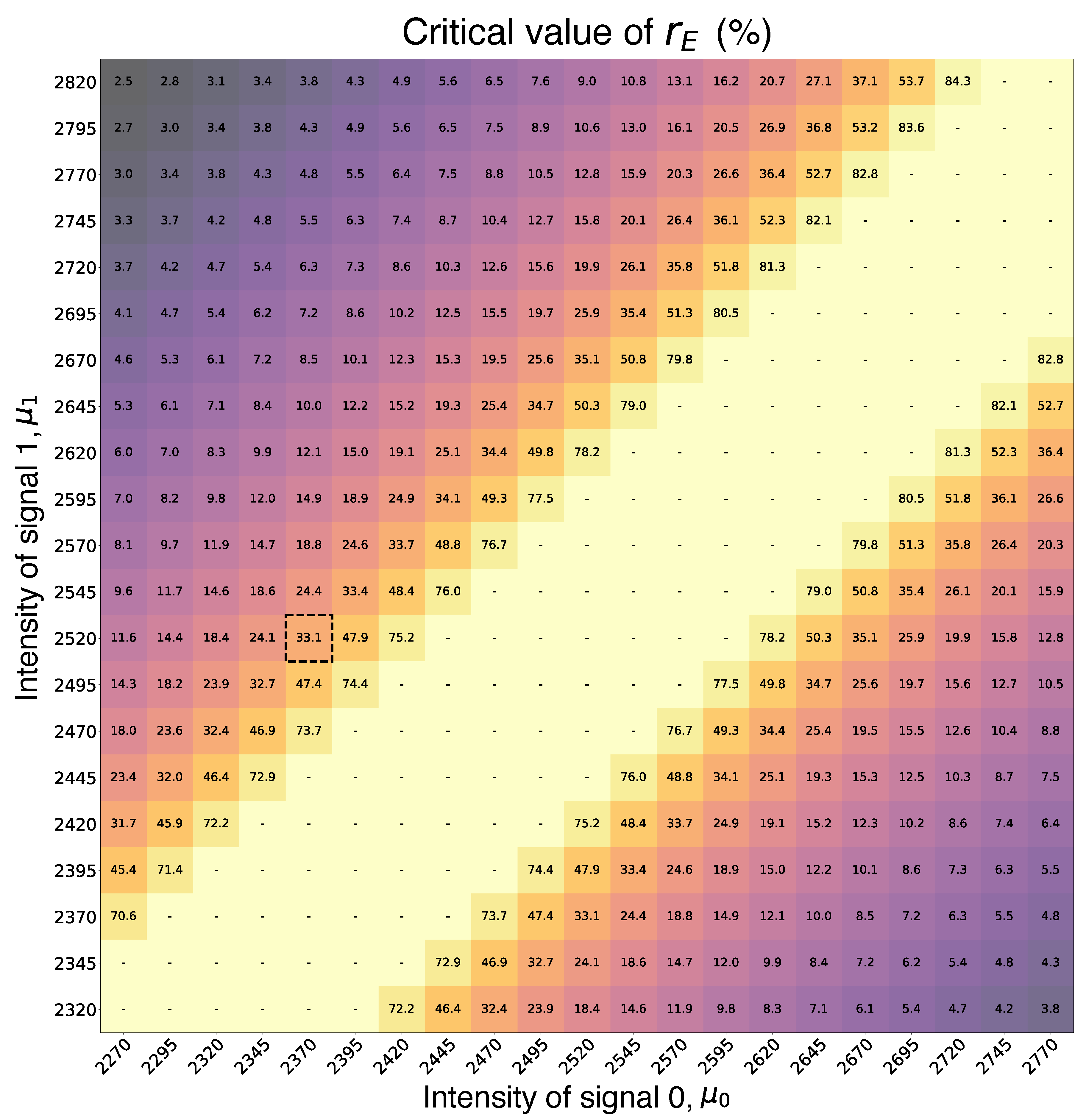

Table 1.
Results of NIST Statistical Tests for Randomness. For each test in the NIST Statistical Test Suite, the table reports the test name, the corresponding P-value, the proportion of sequences that passed (i.e., the fraction of sequences with P-values at or above the significance level), and the overall pass/fail verdict. The proportion is evaluated against an expected confidence interval—computed using a normal approximation to the binomial distribution for large sample sizes—to determine if the randomness criteria are met.
| Statistical Test | P-value | Proportion | Result |
|---|---|---|---|
| Frequency | 0.64 | 1.0 | SUCCESS |
| Block Frequency | 0.83 | 1.0 | SUCCESS |
| Cumulative Sums | 0.16 | 1.0 | SUCCESS |
| Runs | 0.44 | 1.0 | SUCCESS |
| Longest Run | 0.28 | 0.9 | SUCCESS |
| Rank | 0.83 | 1.0 | SUCCESS |
| FFT | 0.44 | 1.0 | SUCCESS |
| Non Overlapping Template | 0.06 ÷ 0.98 | 0.9 ÷ 1.0 | SUCCESS |
| Overlapping Template | 0.28 | 0.9 | SUCCESS |
| Universal | 0.16 | 1.0 | SUCCESS |
| Approximate Entropy | 0.16 | 1.0 | SUCCESS |
| Random Excursions | 0.14 ÷ 0.99 | 1.0 | SUCCESS |
| Random Excursions Variant | 0.06 ÷ 0.98 | 1.0 | SUCCESS |
| Serial | 0.83 ÷ 0.96 | 1.0 | SUCCESS |
| Linear Complexity | 0.96 | 1.0 | SUCCESS |
Disclaimer/Publisher’s Note: The statements, opinions and data contained in all publications are solely those of the individual author(s) and contributor(s) and not of MDPI and/or the editor(s). MDPI and/or the editor(s) disclaim responsibility for any injury to people or property resulting from any ideas, methods, instructions or products referred to in the content. |
© 2025 by the authors. Licensee MDPI, Basel, Switzerland. This article is an open access article distributed under the terms and conditions of the Creative Commons Attribution (CC BY) license (http://creativecommons.org/licenses/by/4.0/).
Copyright: This open access article is published under a Creative Commons CC BY 4.0 license, which permit the free download, distribution, and reuse, provided that the author and preprint are cited in any reuse.


