
Submitted:
06 March 2025
Posted:
07 March 2025
You are already at the latest version
Abstract
In this paper, based on the novel generalized Hamilton-real (GHR) calculus, we propose for the first time a quaternion Nesterov’s accelerated projected gradient algorithm for computing the dominant eigenvalue and eigenvector of quaternion Hermitian matrices. By introducing momentum terms and look-ahead updates, the algorithm achieves a faster convergence rate. We theoretically prove the convergence of the quaternion Nesterov’s accelerated projected gradient algorithm. Numerical experiments show that the proposed method outperforms the quaternion projected gradient ascent method and the traditional algebraic methods in terms of computational accuracy and runtime efficiency.
Keywords:
GHR calculus
; Principal eigenvalues
; Quaternion Hermitian matrix
; Nesterov’s accelerated gradient method
MSC: 15A18; 15B57; 65F10; 65F15
1. Introduction
In 1843, Sir William Rowan Hamilton [9] introduced quaternions in an effort to expand the concept of complex numbers into spaces of higher dimensions. Quaternions and quaternion matrices play a critical role in many applications, such as quantum mechanics, computer graphics, quaternion principal component analysis (QPCA) and image processing [2,11,23,24]. Due to the non-commutative property of quaternion multiplication, the eigenvalues of quaternion matrices are distinguished into left and right types, with the right eigenvalue problem having garnered widespread attention[4,6,14,16,25].
In recent years, a series of numerical methods have been developed to compute the eigenvalues of quaternion matrices, particularly focusing on the eigenvalue problems of Hermitian matrices. These numerical methods can be broadly categorized into three classes: The first class involves direct quaternion arithmetic operations. For instance, Bunse-Gerstner proposed a quaternion QR algorithm for solving the right eigenvalue problem of quaternion matrices [1]. However, due to the complexity of quaternion arithmetic, this algorithm requires significant computational effort. The second class is based on the real or complex counterparts of quaternion matrices. By studying the real or complex counterpart structures and properties of quaternion matrices, and leveraging stable orthogonal transformations, real or complex structure-preserving methods have been developed to solve the right eigenvalue problem of quaternion Hermitian matrices [8,10]. The third class is based on the real counterparts of quaternion matrices, leading to the development of numerous structure-preserving iterative algorithms. Examples include the explicitly restarted quaternion Arnoldi Method (ERQAM) [18], designed to compute standard right eigenpairs of general quaternion matrices, and a novel quaternion power method introduced in [13] for computing the dominant standard right eigenvalue and its corresponding eigenvector. Structure-preserving methods exhibit significant advantages in terms of storage space and computational efficiency.
In the field of quaternion optimization, significant progress has been made with the generalized HR calculus (GHR) [20,21,22]. GHR leverages quaternion rotations within a general orthogonal system, offering a way to compute the derivatives and gradients of functions with quaternion variables, thereby providing a solid theoretical foundation for the development of quaternion optimization methods. Subsequently, based on the generalized HR calculus (GHR), Diao et al. [3] proposed a gradient projection algorithm for maximizing the quaternion Rayleigh quotient under unit constraints. This algorithm demonstrated good performance and contributed to the development of quaternion optimization algorithms.
In this paper, we first equivalently transform the principal eigenvalue problem of quaternion Hermitian matrices into a maximization optimization problem over the quaternion skew field. Leveraging generalized HR calculus, we propose a quaternion Nesterov’s accelerated gradient projection algorithm to solve it. Subsequently, we conduct a convergence analysis of the quaternion Nesterov’s accelerated gradient projection algorithm, proving that a real differentiable function with Lipschitz continuous gradient possesses a quadratic upper bound. Furthermore, we demonstrate that the algorithm possesses a convergence rate of . Finally, we compare our algorithm with two other methods, and numerical experiments indicate that our algorithm exhibits superior performance in terms of both accuracy and time efficiency.
The rest of this paper is organized as follows. Section 2 introduces some basic notations and fundamental properties of quaternions, including definitions of quaternion modulus, similarity, and rotation, with a particular emphasis on reviewing the relevant definitions and properties of generalized HR integrals. In Section 3, we design a quaternion Nesterov accelerated gradient projection algorithm to solve the principal eigenvalue and corresponding eigenvector of quaternion Hermitian matrices. Section 4 provides a convergence analysis of the quaternion Nesterov accelerated gradient projection algorithm. In Section 5, we conduct numerical experiments to validate the proposed method. Finally, in Section 6, we summarize this paper.
2. Preliminaries
In this section, some quaternion notations and basic definitions are introduced, which will be used in the rest of the paper.
2.1. Notations
Throughout this paper, to distinguish scalars, vectors, real or complex matrices and quaternion matrices, scalars will be denoted by lower case Greek letters, e.g., , , quaternions will be denoted by lowercase letters, e.g., , and quaternion vectors are denoted by , real or complex matrices will be defined by uppercase letters, e.g., , and quaternion matrices will be denoted by bold uppercase letters, e.g., . denotes the identity quaternion matrix. The operators and represent transpose and conjugate transpose, respectively. The MATLAB function command will be denoted by typewriter letters, e.g., .
2.2. Quaternions and Quaternion Matrices
Denote the set of quaternions as
where are three imaginary units of quaternions, satisfying
The scalar (real) part of is denoted by . And the vector (imaginary) part of is denoted by . A quaternion is called imaginary when its real part is equal to zero. The multiplication of quaternions adheres to the distributive law but is noncommutative.
The zero element in is and the unit element is . For any , the conjugate of a quaternion is defined as
The magnitude of is , it follows that the inverse of a nonzero quaternion is given by .
Two quaternions and are said to be similar if there exists a nonzero quaternion such that , this is written as . Obviously, and are similar if and only if there is a unit quaternion such that , and two similar quaternions have the same norm. It is routine to check that ∼ is an equivalence relation on the quaternions. We denote by the equivalence class containing . If , then and are similar, namely, .
Quaternions can also be expressed in polar form as , where is a pure unit quaternion and denotes the angle (or argument) of the quaternion. Next, we will introduce the quaternion rotation and involution operators.
Definition 1
(Quaternion rotation[19]). For any quaternion , the transformation
geometrically describes a three-dimensional rotation of the vector part of by an angle about the vector part of μ, where is any nonzero quaternion.
Specifically, if in (2) is an imaginary unit, then the quaternion rotation (2) reduces to quaternion involution [5], defined by
where . Below, we will list some properties of quaternion rotation, including
and
Note that the representation in (1) can be extended to a general orthogonal basis , where the following properties hold [19]:
Denote the set of quaternion matrices as
The conjugate transpose of is . We say that a square quaternion matrix is normal if ; Hermitian if , i.e. and ; Unitary if , where is the identity matrix; Invertible (nonsingular) if there exists a matrix such that . In this case, we denote . We have if and are invertible, and if is invertible.
2.3. GHR calculus
We now introduce the generalized HR derivatives which comprise both the product and chain rules, see [20,22] for more details.
Definition 2
(real-differentiability [20]). Let , then a function is called real differentiable when and are differentiable with respect to the real variables and , respectively.
Definition 3
(GHR derivatives [20]). If is real differentiable, then the GHR derivatives of with respect to and are defined as
and
where , , and are the partial derivatives of f with respect to and , while the set is an orthogonal basis of .
Definition 4
(Quaternion gradient[20]). Let and , then the two quaternion gradients of f are defined as
and
Based on the definitions of GHR provided above, we consider a simple quadratic function , where and is a quaternion Hermitian matrix, then the gradient of this function f is given by
in which is the steepest ascent direction [22].
3. Quaternion Nesterov’s Accelerated Gradient (QNAG)
In this section, we will introduce the quaternion Nesterov accelerated projected gradient algorithm. To this end, we first review the definition related to the eigenvalue of quaternion Hermitian matrices.
Definition 5.
Let be a quaternion Hermitian matrix. Then is called an eigenvalue of if there exists a nonzero vector such that
Here is called the eigenvector corresponding to the eigenvalue λ.
Due to the non-commutativity of quaternion multiplication, general quaternion square matrices have distinct left and right eigenvalues. However, for a quaternion Hermitian matrix , if has a right eigenvalue and its corresponding eigenvector , it is straightforward to show that
by dividing both sides of the above equation by , we obtain
where (3) represents the Rayleigh quotient on the quaternion skew field. Therefore, the eigenvalues of quaternion Hermitian matrices are all real numbers, and thus there is no distinction between left and right eigenvalues.
Our goal is to compute the principal eigenvalue of a given quaternion Hermitian matrix. By defining the objective function as and imposing the normalization constraint , we can equivalently transform the problem of finding the principal eigenvalue of a given quaternion Hermitian matrix into the following maximization optimization problem on the quaternion skew-field
The above problem (4) can be addressed using the quaternion gradient projection algorithm. Since the introduction of the Nesterov’s Accelerated Gradient (NAG) method [15], the incorporation of momentum has become a conventional approach to overcome the shortsighted issue in gradient algorithms [7,12]. To tackle the problem (4), we propose a quaternion Nesterov’s accelerated gradient projection algorithm (QNAG). Given an initial point , and set , the QNAG method repeats, for ,
where and are the step-size and momentum parameters, respectively. When the momentum parameter , QNAG simplifies to standard gradient ascent (GA). When it is possible to achieve accelerated rates of convergence for certain combinations of and in the deterministic setting. The framework of the proposed algorithm is detailed below.
Remark 1.
After obtaining the principal eigenvalue and its corresponding eigenvector of the quaternion Hermitian matrix, we can employ a deflation technique by updating and continue to apply the QNAG algorithm. By repeating this process, all eigenvalues and their corresponding eigenvectors can be obtained.
4. Convergence Analysis of QNAG
In this section, we will theoretically prove the convergence properties of the quaternion Nesterov’s accelerated gradient projection algorithm. We begin our analysis with the following Lemma 1.
Lemma 1.
If is a real differentiable and gradient Lipschitz continuous function with constant ,
| Algorithm 1: Quaternion Nesterov’s Accelerated Gradient (QNAG). |
|
Then, f has the following quadratic upper bound
Proof.
For any , let . Define the parameterized path for . Then the difference in the function can be expressed as
Using the chain rule, the derivative corresponds to the directional derivative of f along . In terms of the quaternion gradient [22], this is given by
Thus, the function difference becomes
Subtracting the linear term from both sides
then using the absolute value inequality and the Cauchy-Schwarz inequality, we have
By the gradient Lipschitz condition, we have
substituting the above inequality into the integral (7), we get
Thus, for all , we have
This completes the proof of the quadratic upper bound.
□
Theorem 1.
Let is a real differentiable and gradient Lipschitz continuous function with constant . If the step size and momentum parameter , then
is true for any , where and C is a constant related to the initial conditions.
Proof.
From Lemma 1, for the update , we have
Substituting , we derive
Choosing , this simplifies to
After projecting onto the unit sphere, . Applying Lemma 1 again to and , we get
By the optimality condition of the projection, we have
which implies
Next, we consider the bound of the projection error
Combining and normalizing such that , we obtain
which implies that
Thus, the projection error in (9) is a higher-order term, we get
We then define the Lyapunov function as
where the auxiliary sequence satisfies , and follows the update rule
Our goal is to prove that . Compute , we obtain
For the term , we have
Thus we have
Suppose that
Substituting this into the Lyapunov difference and combining with (10), we arrive at
Using and , we simplify
After algebraic manipulation, we show that
From and , we have
Letting , we conclude
where is a constant related to the initial setup. Algorithm 1 achieves an convergence rate. This completes the proof.
□
5. Numerical Experiments
In this section, we provide numerical examples to demonstrate the feasibility and effectiveness of the quaternion Nesterov’s accelerated gradient projection algorithm for the eigenvalue problem of quaternion Hermitian matrices. In the specific implementation of Algorithm 1, we set the constant step size and momentum parameter to and , respectively.
All the experiments are performed under Windows 11 and MATLAB version 23.2.0.2365128 (R2023b) with an AMD Ryzen 7 5800H with Radeon Graphics CPU at 3.20 GHz and 16 GB of memory.
Example 1.
Given quaternion matrix with
and
In this experiment, we employ the quaternion Nesterov’s accelerated gradient (QNAG) method (Algorithm 1) to compute all eigenvalues of , which are , with their corresponding eigenvectors being
Additionally, we obtain the following three residuals:
It is evident that the residuals are controlled within an ideal range, demonstrating the feasibility and effectiveness of Algorithm 1 in computing the eigenvalues of quaternion Hermitian matrices.
Example 2.
In this experiment, we utilize MATLAB’s built-in functions to randomly generate three quaternion Hermitian matrices of different sizes and compare Algorithm 1 with the QPGA algorithm [3] and theeigfunction in the Quaternion Toolbox for MATLAB (QTFM)[17].
We first test the performance of Algorithm 1, QPGA, and the eig function in computing the principal eigenvalues of three different types and sizes of quaternion Hermitian matrices. The numerical experimental results are presented in Table 1, which includes three evaluation metrics: the number of iterations, residuals, and runtime. Superior results are highlighted in bold. It can be observed that Algorithm 1 outperforms the other algorithms in terms of the number of iterations, problem residuals, and runtime, demonstrating significant advantages when computing large-scale quaternion Hermitian matrices.
Subsequently, we plotted the variation curves of the objective function values for the first 50 iterations of Algorithm 1 and the QNGA algorithm, as shown in Figure 1. It is evident that our algorithm achieves a faster increase in the objective function, demonstrating higher efficiency in obtaining the maximum eigenvalue.
Figure 2 illustrates the residual variation curves generated by Algorithm 1 and the QNGA algorithm with respect to the number of iterations. Across the tested matrix dimensions, our algorithm consistently achieves higher accuracy and efficiency.
6. Conclusions
In this paper, leveraging the innovative generalized Hamilton-real (GHR) calculus, we have introduced a novel quaternion Nesterov’s accelerated projected gradient algorithm designed to compute the dominant eigenvalue and corresponding eigenvector of quaternion Hermitian matrices. The incorporation of momentum terms and look-ahead updates has enabled the algorithm to attain an accelerated convergence rate. Theoretical analysis has confirmed the convergence of the quaternion Nesterov’s accelerated projected gradient algorithm. Empirical results from numerical experiments indicate that the proposed method surpasses both the Quaternion Projected Gradient Ascent (QPGA) and conventional algebraic approaches in terms of both computational precision and efficiency in runtime.
Author Contributions
Shan-Qi Duan wrote the main manuscript text and performed the experiment. Qing-Wen Wang contributed to the conception of the study and helped to improve this manuscript with constructive suggestions. Xue-Feng Duan made a lot of useful suggestions. All authors reviewed the manuscript.
Funding
This work is supported by the National Natural Science Foundation of China under Grant 12371023.
Data Availability Statement
Data is contained within the article.
Conflicts of Interest
The authors declare no conflict of interest.
References
- Bunse-Gerstner, A. , Byers, R., Mehrmann, V. A quaternion QR algorithm. Numer. Math. 1989, 55, 83–95. [Google Scholar]
- De Leo, S. , Scolarici, G. Right eigenvalue equation in quaternionic quantum mechanics. J. Phys. A Math. Gen. 2000, 33, 2971. [Google Scholar] [CrossRef]
- Diao, Q. , Liu, J., Zhang, N., Xu, D. An iterative algorithm for quaternion eigenvalue problems in signal processing. IEEE Signal Process. Lett. 2024, 31, 2505–2509. [Google Scholar]
- Duan, S.Q. , Wang, Q.W., Duan, X.F. On Rayleigh quotient iteration for the dual quaternion Hermitian eigenvalue problem. Mathematics 2024, 12. [Google Scholar] [CrossRef]
- Ell, T.A. , Sangwine, S.J. Quaternion involutions and anti-involutions. Comput. Math. Appl. 2007, 53, 137–143. [Google Scholar] [CrossRef]
- Farid, F. , Wang, Q.W., Zhang, F. On the eigenvalues of quaternion matrices. Lin. Multilin. Alg. 2011, 59, 451–473. [Google Scholar]
- Ghadimi, S. , Lan, G. Accelerated gradient methods for nonconvex nonlinear and stochastic programming. Math. Program. 2016, 156, 59–99. [Google Scholar]
- Guo, Z. , Jiang, T., Vasil’ev, V., Wang, G. Complex structure-preserving method for schrödinger equations in quaternionic quantum mechanics. Numer. Algorithms 2024, 97, 271–287. [Google Scholar]
- Hamilton, W.R. Elements of Quaternions. Longmans, Green (1866).
- Jia, Z. , Wei, M., Ling, S. A new structure-preserving method for quaternion Hermitian eigenvalue problems. J. Comput. Appl. Math. 2013, 239, 12–24. [Google Scholar]
- Jiang, T. , Chen, L. An algebraic method for schrödinger equations in quaternionic quantum mechanics. Comput. Phys. Commun. 2008, 178, 795–799. [Google Scholar]
- Li, H. , Peng, Z., Pan, C., Zhao, D. Fast gradient method for low-rank matrix estimation. J. Sci. Comput. 2023, 96, 41. [Google Scholar]
- Li, Y. , Wei, M., Zhang, F., Zhao, J. On the power method for quaternion right eigenvalue problem. J. Comput. Appl. Math. 2019, 345, 59–69. [Google Scholar]
- Macías-Virgós, E. , Pereira-Sáez, M., Tarrío-Tobar, A.D. Rayleigh quotient and left eigenvalues of quaternionic matrices. Linear Multilinear Algebra 2023, 71, 2163–2179. [Google Scholar]
- Nesterov, Y. A method for unconstrained convex minimization problem with the rate of convergence O(1/k2). Dokl. Akad. Nauk. SSSR 1983, 269, 543. [Google Scholar]
- Rodman, L. Topics in quaternion linear algebra. Princeton University Press (2014).
- Sangwine, S.J., Bihan, N.L. Quaternion toolbox for matlab, version 2 with support for octonions. Software library available at: http: //qtfm.sourceforge.net/ (2013).
- Wang, Q.W. , Wang, X.X. Arnoldi method for large quaternion right eigenvalue problem. J. Sci. Comput. 2020, 82, 58. [Google Scholar]
- Ward, J.P. Quaternions and Cayley numbers: Algebra and applications, vol. 403. Springer Science & Business Media (2012).
- Xu, D. , Jahanchahi, C., Took, C.C., Mandic, D.P. Enabling quaternion derivatives: The generalized hr calculus. R. Soc. Open Sci. 2015, 2, 150255. [Google Scholar] [CrossRef]
- Xu, D. , Mandic, D.P. The theory of quaternion matrix derivatives. IEEE Trans. Signal Process. 2015, 63, 1543–1556. [Google Scholar]
- Xu, D. , Xia, Y., Mandic, D.P. Optimization in quaternion dynamic systems: Gradient, Hessian, and learning algorithms. IEEE Trans. Neural Netw. Learn. Syst. 2015, 27, 249–261. [Google Scholar]
- Yu, C.E. , Liu, X., Zhang, Y. A new complex structure-preserving method for QSVD. J. Sci. Comput. 2024, 99, 37. [Google Scholar]
- Zeng, R. , Wu, J., Shao, Z., Chen, Y., Chen, B., Senhadji, L., Shu, H. Color image classification via quaternion principal component analysis network. Neurocomputing 2016, 216, 416–428. [Google Scholar]
- Zhang, F. Quaternions and matrices of quaternions. Linear Algebra Its Appl. 1997, 251, 21–57. [Google Scholar] [CrossRef]
Figure 1.
Variation curve of the objective function value with respect to the number of iterations for Algorithm 1 on a 1000-order quaternion Hermitian matrix.
Figure 1.
Variation curve of the objective function value with respect to the number of iterations for Algorithm 1 on a 1000-order quaternion Hermitian matrix.
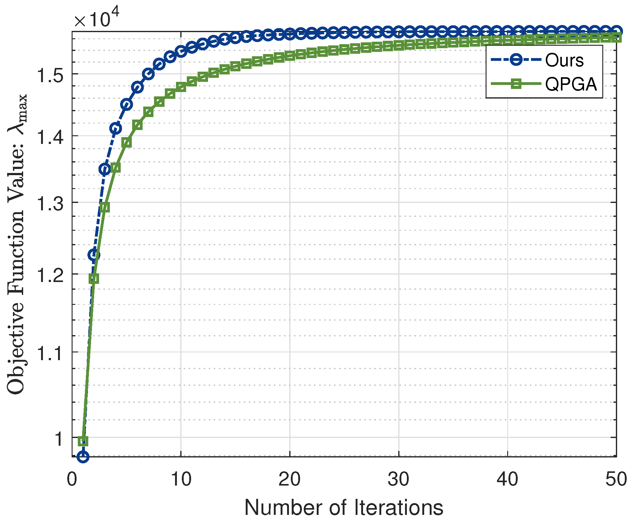
Figure 2.
Comparison of fixed iteration steps and residual variation curves between Algorithm 1 and QPGA for solving Problem (4), with quaternion Hermitian matrix sizes of order 300 and 1000 on the left and right, respectively.
Figure 2.
Comparison of fixed iteration steps and residual variation curves between Algorithm 1 and QPGA for solving Problem (4), with quaternion Hermitian matrix sizes of order 300 and 1000 on the left and right, respectively.
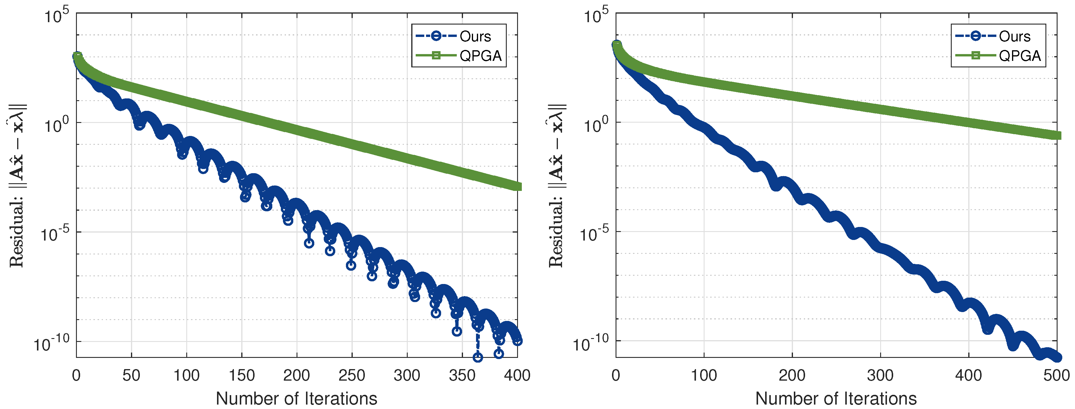

Table 1.
Numerical comparison results of the QNAG algorithm, QPGA algorithm, and eig function for computing the principal eigenvalue and its corresponding eigenvector of three types of quaternion Hermitian matrices.
Table 1.
Numerical comparison results of the QNAG algorithm, QPGA algorithm, and eig function for computing the principal eigenvalue and its corresponding eigenvector of three types of quaternion Hermitian matrices.
| Matrix type | n | Ours | QPGA [3] | eig [17] | |||||
| IT | Residual | CPU(s) | IT | Residual | CPU(s) | Residual | CPU(s) | ||
| General | 300 | 453 | 4.5453e-12 | 0.6667 | 1764 | 9.9457e-12 | 2.4857 | 9.6329e-12 | 3.4420 |
| Hermitian | 500 | 432 | 9.4172e-12 | 2.6465 | 1368 | 9.8076e-12 | 8.2786 | 3.3852e-11 | 24.6503 |
| 1000 | 461 | 8.2506e-12 | 10.4795 | 1592 | 9.8945e-12 | 36.1470 | 2.1115e-10 | 373.4246 | |
| Positive | 300 | 434 | 1.6844e-12 | 0.6420 | 1141 | 9.8121e-12 | 1.7283 | 1.5353e-11 | 3.3504 |
| Semi-definite | 500 | 454 | 9.2637e-12 | 2.6836 | 2020 | 9.9177e-12 | 11.7135 | 1.9891e-11 | 24.6779 |
| 1000 | 485 | 8.2055e-12 | 10.6467 | 1943 | 9.9733e-12 | 42.3868 | 1.7807e-10 | 362.1100 | |
| Positive | 300 | 419 | 1.5814e-12 | 0.6079 | 1615 | 9.8821e-12 | 2.2746 | 3.9411e-11 | 3.3670 |
| Definite | 500 | 457 | 9.9405e-12 | 2.7210 | 1530 | 9.5587e-12 | 9.1385 | 2.3945e-11 | 24.3842 |
| 1000 | 503 | 7.8888e-12 | 11.2300 | 2636 | 9.9721e-12 | 56.6146 | 7.2911e-11 | 379.0733 | |
Disclaimer/Publisher’s Note: The statements, opinions and data contained in all publications are solely those of the individual author(s) and contributor(s) and not of MDPI and/or the editor(s). MDPI and/or the editor(s) disclaim responsibility for any injury to people or property resulting from any ideas, methods, instructions or products referred to in the content. |
© 2025 by the authors. Licensee MDPI, Basel, Switzerland. This article is an open access article distributed under the terms and conditions of the Creative Commons Attribution (CC BY) license (http://creativecommons.org/licenses/by/4.0/).
Copyright: This open access article is published under a Creative Commons CC BY 4.0 license, which permit the free download, distribution, and reuse, provided that the author and preprint are cited in any reuse.


