1. Introduction
With urban populations rapidly increasing, cities are facing unprecedented challenges in managing waste efficiently. Effective waste management is crucial not only for public health and well-being but also for environmental sustainability and economic development. Traditional waste management systems often struggle with inefficiencies, leading to overflowing bins, increased operational costs, and higher greenhouse gas emissions. These issues underscore the need for innovative solutions to optimize waste collection and reduce environmental impact.
The way waste is managed has a direct impact on the quality of life in cities and also on compliance with global environmental commitments, such as the Sustainable Development Goals (SDGs) [
1] defined by the United Nations (UN). Among the most relevant SDGs are SDG 11 (Sustainable cities and communities) and SDG 12 (Responsible consumption and production), which encourage a more sustainable and efficient approach to waste management and resource use.
The European Commission has been reinforcing the importance of efficient and sustainable urban waste management, with various deliberations and strategies to promote the circular economy and reduce the environmental impact of cities. The “Circular Economy Package” [
2], one of the European Union’s main legislative initiatives, defines a set of targets and measures to improve waste management, including reducing the waste of resources, promoting recycling, and eliminating waste from landfills. This package encourages municipalities to adopt more effective waste management practices that not only improve environmental quality but also contribute to economic development and the creation of green jobs.
The “Strategy for Plastics in the Circular Economy” [
3] is another example of how the European Commission is promoting innovative solutions for waste management. This strategy focuses particularly on reducing the use of single-use plastics and improving plastic recycling. In addition, the European Commission has been promoting digitalization and technological innovation in the municipal waste management sector, encouraging municipalities to adopt smart technologies that can optimize waste collection and transport processes. The 2020 “Circular Economy Strategy” [
4], for example, highlights the role of technological innovation, including the Internet of Things (IoT), to improve efficiency in waste management, enabling more efficient collection and reducing the environmental impact of urban waste management systems.
The use of IoT technologies to monitor waste garbage cans in real-time represents one of the most innovative and effective solutions for urban waste management. Using fill-level sensors, bins can be monitored in real-time, allowing collection services to be notified as soon as bins are full. This intelligent management system makes it possible to optimize collection vehicle routes, scheduling collection only when the containers are full. Additionally, it can include an alert mechanism that notifies when bins are nearing capacity, allowing for proactive scheduling of future collection visits to prevent overflow and ensure timely waste management.
With this approach, the municipality can significantly reduce operating costs, such as vehicle fuel, and reduce greenhouse gas emissions, which contributes to the fight against climate change.
This strategy not only helps to optimize collection logistics but also positively impacts cities’ environmental sustainability. Reducing unnecessary journeys by collecting vehicles means reducing fuel consumption and carbon dioxide emissions, in line with global decarbonization objectives and the European Union’s climate targets. Furthermore the implementation of IoT systems contributes to greater control over waste management, allowing municipalities to make informed decisions about optimizing logistics and collection planning, which results in more efficient and sustainable management of municipal waste.
The relationship between smart municipal waste management and SDGs is clear. SDG 11, which promotes sustainable cities and communities, and SDG 12, which promotes responsible consumption and sustainable production, are directly benefited by the implementation of systems such as the one described. These systems promote more efficient waste management and encourage a more rational use of resources, avoiding waste and encouraging recycling. Besides, reducing the environmental impact of urban activities, namely by reducing emissions associated with waste transportation, contributes to the objectives of the Paris Agreement on climate change, which aims to limit global warming to 1.5 °C above pre-industrial levels.
Moreover, the implementation of IoT technologies in municipal waste management can also generate significant financial savings for municipalities. The efficient use of resources, including the optimization of collection routes and the reduction of operating costs, contributes to a more economical and efficient management of urban services. The integration of IoT sensors and networks into municipal waste management systems also allows for the development of more innovative and digital solutions that can be applied to other areas of municipal management, such as air, water, and energy quality control, contributing to the creation of smart cities.
The proposed system, which integrates ToF sensors, Raspberry Pi, and ESP32-S3, offers a comprehensive, reliable, and scalable approach to monitoring and data transmission. This solution is particularly suitable for smart city applications due to its cost-effectiveness, scalability, flexibility, real-time monitoring capabilities, reliability, portability, and compact design. The high precision of the ToF sensors ensures accurate measurements, which is vital for effective waste management.
In short, the adoption of IoT technologies for urban waste management represents a significant advance in the way municipalities can manage waste, reducing environmental impact, promoting sustainability, and contributing to the achievement of the UN’s Sustainable Development Goals. By integrating smart solutions into waste management, municipalities not only improve the quality of life of their citizens but also contribute to building greener, more efficient, and sustainable cities.
This study aims to demonstrate the possibility of using ToF sensors connected to an IoT network for real-time monitoring of waste bins, through their height (full or empty) and volume. When collection services are notified, via ToF sensors, that bins are full, collection can be scheduled accurately, avoiding unnecessary journeys. The experiment we carried out involved an modified garbage can, mapping it using the ToF sensor (supported by a microcontroller to acquire sensor data), then sending the data via WiFi to a gateway and subsequently to an Internet of Things (IoT) cloud. The results are recorded and displayed.
The article provides a theoretical background on ToF technology, discusses its current state, and references related works in
Section 2.
Section 3 outlines the materials and methods used in the research. The results obtained are presented in
Section 5. Finally, Section 6 concludes the article and offers insights into future work. The article provides a theoretical background on ToF technology, discusses its current state, and references related works in
Section 2.
Section 3 outlines the materials and methods used in the research. The results obtained are presented in
Section 5. Finally, Section 6 concludes the article and offers insights into future work.
2. Background Theory and State of the Art
This section explores the technology behind ToF cameras. Starting with an explanation of their structure and operating principles. Following this, we compare ToF cameras with other technologies to highlight their unique advantages. In
Section 2.2, we will provide an overview of the latest advancements in the field and delve into relevant research and studies that complement this discussion.
2.1. Background Theory
The ToF camera resembles a traditional digital camera, with a lens focusing light on an image sensor, which is a two-dimensional array of photosensitive pixels. However, unlike typical digital cameras, a ToF camera features an active light source to illuminate the scene. The camera captures reflected light from the scene, with each pixel in parallel calculating depth data to create a complete depth map. Light-emitting diodes (LEDs) are commonly used as the light source due to their rapid response time. Most commercial ToF sensors use Near-InfraRed (NIR) wavelengths, around 850 nm, which are invisible to the human eye and allow high reflectance across various materials without interfering with vision [
5].
Pixel implementations for image sensors vary according to the operational principle discussed further in the next section. Most current ToF systems are analog, using photodetectors and capacitors to collect and store charge from light pulses before converting it to a digital signal. Fully digital ToF cameras are also under development, using Single Photon Avalanche Diodes (SPADs) that can detect individual photons. Digital ToF systems help reduce noise linked to analog signals and the conversion process [
5]. SPADs are specialized photo detectors offering high sensitivity to low light, capable of detecting single photons. Operating in avalanche mode—biased above their breakdown voltage—SPADs amplify each detected photon into a cascade of charge carriers, creating a detectable current pulse. This amplification enables SPADs to sense extremely faint light levels, down to individual photons [
6].
The timing precision of SPADs is critical for applications like ToF sensors and Light Detection and Ranging (LiDAR), where accurate distance calculations depend on detecting light pulses. By measuring the time delay between a photon’s emission and its return after reflecting from an object, SPADs calculate distances with high temporal resolution. This capability is especially valuable in robotics, 3D scanning, and automotive sensing, where detailed depth information is crucial. However, SPADs have some limitations, such as after pulsing, where a SPAD remains sensitive after detecting a photon, potentially causing false counts, and dead time, which limits the detection rate, especially in high-light or rapid-detection environments [
5] [
6].
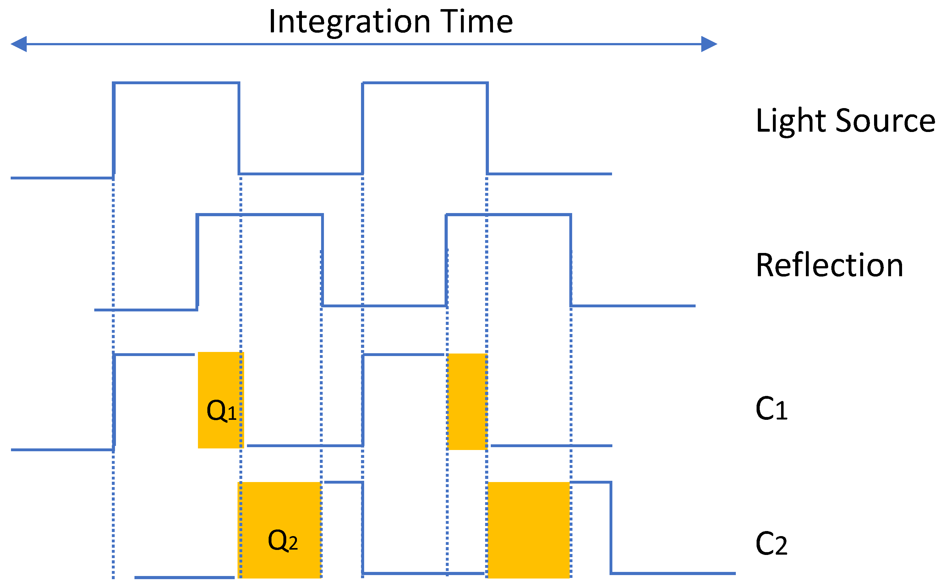
The fundamental operating principle of ToF cameras involves illuminating a scene with a modulated light source and measuring the light that reflects to the sensor. Since the speed of light is constant, the distance to the object from which the light was reflected can be determined by calculating the time difference between the emitted and returning light signals. ToF cameras use two primary illumination techniques: pulsed light and Continuous Wave (CW) modulation.
In pulsed light ToF, short bursts of light are emitted, and the time taken for the light to return is measured to calculate distance. In CW modulation, the light source emits a continuous, sinusoidally modulated wave, and the phase shift between the emitted and received light is used to compute the depth information.
In the pulsed method, depth measurement is straightforward. The illumination unit quickly switches on and off, creating short pulses of light. A timer is activated when the light pulse is emitted and stops when the reflected light is detected by the sensor. The distance,
d, to the object, is then calculated based on the elapsed time, as described in [
7].
where
∆t is the round-trip time of the light pulse and
c is the speed of light. However, the ambient illumination usually contains the same wavelengths as the light source of the ToF camera. The light captured by the camera consists of both emitted light and ambient light. This mixture can cause inaccuracies in calculating distances. To address this, a measurement is taken when the illumination unit is switched off, allowing the ambient background to be subtracted from the overall signal. This adjustment is managed by using the outgoing light signal as a control for the sensor detector.
Additionally, each short light pulse contains a relatively low amount of energy [
6], and due to imperfections in the system components [
8], the signal received is prone to noise. To improve the signal-to-noise ratio (SNR), multiple cycles of these pulses—often millions—are recorded over a specific period. The final depth information is derived from the average of these cycles. This recording period is known as the Integration Time (IT) [
9].
Figure 1 illustrates the concept of this pulsed modulation method. By using an integration time interval of
∆t and two sampling windows (C
1 and C
2) that are out of phase, the averaged distance can be calculated [
9].
where
Q1 and
Q2 are the accumulated electrical charges received over the integration time.
The depth resolution achievable with the pulsed method is constrained by the speed of the camera’s electronics. Based on equation (1), achieving a depth resolution of 1 mm would require a light pulse lasting approximately 6.6 picoseconds. However, the rise and fall times, as well as the repetition rates of current LEDs and laser diodes, impose practical limitations on generating such short pulses [
8]. Moreover, reaching these speeds in the receiver circuit is challenging with today’s silicon-based technology, especially at room temperature [
9].
In the Continuous-Wave (CW) method, instead of directly measuring the round-trip time of a light pulse, the CW modulation method determines the phase difference between sent and received signals. In this approach, the light source is modulated by adjusting its input current, creating a waveform signal [
8]. While various modulation shapes can be used, square or sinusoidal waves are the most common [
10]. The CW modulation technique reduces the requirements for the light source, enabling a finer depth resolution than is possible with pulsed light.
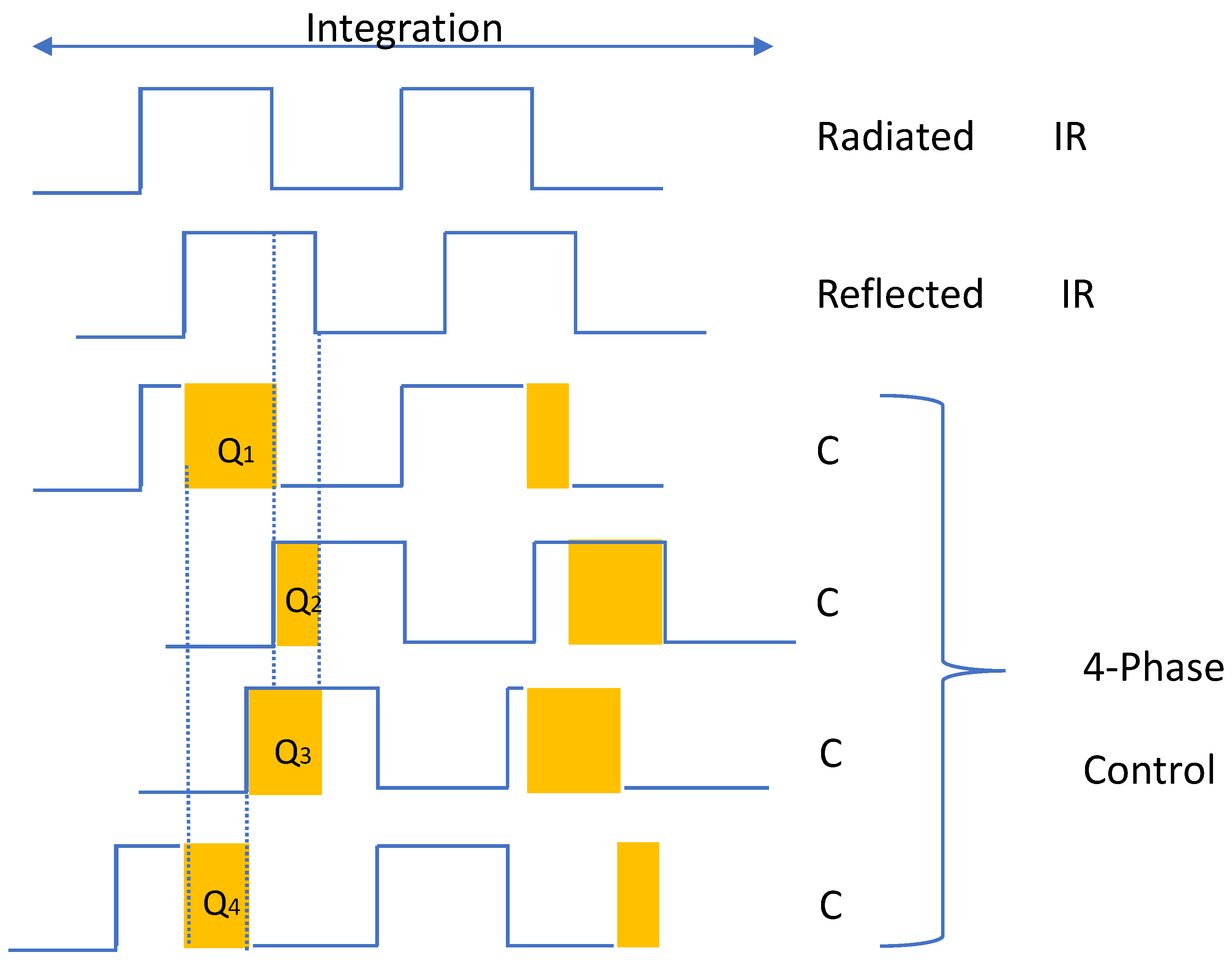
There are multiple ways to demodulate the received signal and extract its amplitude and phase information. A traditional approach involves calculating the cross-correlation function between the original modulation signal and the returned signal [
10]. This cross-correlation can be obtained by measuring the returned signal at specific phases, which can be implemented using mixers and low-pass filters in the detector. A more efficient alternative is synchronous sampling, where the modulated returned light is sampled simultaneously with a reference signal at four different phases (0°, 90°, 180°, and 270°), as shown in
Figure 2 [
10]. This synchronous sampling approach simplifies the circuit design and reduces pixel size, allowing for more pixels on a sensor and thus higher resolution.
Similar to the pulsed method, multiple samples are recorded and averaged to improve the signal-to-noise ratio (SNR). By using four equally spaced sampling windows (
Q1 to
Q4), time by the reference signal (see
Figure 2), the received signal is sampled at different phases over the integration time. Assuming a sinusoidal modulation signal with no harmonic frequencies, Discrete Fourier Transform (DFT) equations can be applied to calculate the phase
ϕ, amplitude A, and offset B as follows [
9] [
10]:
From the phase -, the distance can be finally calculated as [
9]:
The intensity, i.e., amplitude A of the light decreases proportionally to the traveled distance in a known way. Hence, the received amplitude value from (4) can be used as a confidence measure for the distance measurement. Additionally, the reflected signal is often superimposed with background illumination, which causes errors in the measurement. Thus, the offset (5) is used to distinguish the modulated light component from the background light [
10].
When calculating distances from the phase difference as in (6), one important thing has to be considered. Since the modulation signal is periodical, its phase wraps around every phase.
2.2. Relevant Research and Studies
The manuscript [
12] presents the development of a Wireless Sensor Network (WSN) prototype for monitoring solid waste containers, focusing on energy efficiency and reducing operating costs. The authors implemented a system of sensors installed in the containers, capable of measuring the fill level and transmitting the data to a base station via efficient communication. An energy-efficient monitoring algorithm is used to adjust the frequency of readings and transmissions based on changes in the waste level, maximizing battery life. Experimental results showed a significant reduction in energy consumption, with the proposed algorithm extending battery life by around 30% to 40% compared to traditional systems. In addition, the system demonstrated high accuracy in monitoring the fill level of the containers, with error rates of less than 5%. This performance was validated under experimental conditions, including different simulated filling rates. The proposed approach offers a viable solution for improving urban waste management, contributing to the creation of more sustainable and efficient cities.
The manuscript [
13] proposes an intelligent system for the recovery of solid urban waste, to optimize waste management and promote more sustainable practices. The system combines monitoring, data analysis, and decision-making technologies to improve the efficiency of waste collection, separation, and recycling processes. The system uses sensors to monitor container capacity, intelligent algorithms to prioritize collection routes, and analysis tools to promote the separation of higher-value waste. The architecture combines hardware and software devices, including wireless communication modules and interfaces for real-time data visualization.
Experimental results indicate that the implementation of the system has reduced waste management operating costs by around 15% while increasing the efficiency of the collection process by 20%. In addition, the system has contributed to a significant increase in the recycling rate, with improvements of over 25% in some areas. The solution presented demonstrates the potential of intelligent systems in urban solid waste management, contributing to more sustainable practices and greater recovery of recyclable materials.
This article [
14] presents a location-based waste management system using IoT for smart cities. The system was developed to optimize waste collection, reduce costs, and minimize environmental impacts. The proposed architecture uses level sensors installed in the containers to monitor filling capacity, communication modules to transmit the data collected, and a central system that processes this information. The system is complemented with geographical location functionalities, making it possible to prioritize the closest or fullest containers, optimizing collection routes. The experimental results show a significant reduction in fuel consumption and collection times, with an improvement in operational efficiency of between 20% and 25%. In addition, the system showed high accuracy in monitoring filling levels, with errors of less than 5%, and an increase in the overall efficiency of waste management, contributing to the reduction of carbon emissions. The integration of IoT and location-based systems proves to be a promising solution for waste management in smart cities, promoting more sustainable and efficient operations.
The article [
15] by Somu Dhana Satyamanikanta and M. Narayanan presents an innovative solution for urban waste management using sensor and IoT technologies. The proposed system equips waste containers with weight, infrared (IR), and photoelectric sensors, as well as an RFID reader. These devices make it possible to continuously monitor the level of waste, identify discarded objects, and send alerts to local authorities when bins reach maximum capacity. Weight sensors provide accurate information on the volume of waste, while photoelectric sensors identify specific materials, such as electronic components, allowing for quick and targeted interventions. Integration with RFID encourages user participation by sending appreciation messages and personalized data on discarded items. The data collected is transmitted in real-time to the authorities via IoT, ensuring continuous monitoring until the container is emptied. The experimental results showed an accuracy of over 95% in detecting levels and types of waste, as well as a 30% reduction in the authorities’ response time for cleaning the containers. The system also promoted a 20% increase in user participation due to the personalized interaction provided by RFID. It can be concluded that this intelligent solution not only improves waste management efficiency but also contributes to sustainability and quality of life in urban environments.
The article [
16] provides a comparative analysis of ToF and LiDAR sensors specifically for indoor mapping applications. The primary objective of the study is to assess the accuracy, efficiency, and suitability of ToF sensors in relation to conventional LiDAR systems for indoor use. The research methodology involved conducting a series of experimental tests within indoor settings, utilizing both sensor types to gather spatial data. Key parameters evaluated included the accuracy of distance measurements, spatial resolution, response time, and the capability to detect objects under varying environmental conditions. Findings indicated that LiDAR sensors deliver superior accuracy in distance measurement, with an average error margin of approximately 2 cm, whereas ToF sensors exhibited an average error of about 5 cm. Nonetheless, ToF sensors were noted for their cost-effectiveness and lower energy consumption, rendering them a viable option for applications where utmost precision is not essential. Furthermore, ToF sensors proved to be more effective in identifying objects in highly reflective environments, a scenario where LiDAR systems may encounter challenges due to signal saturation. In conclusion, the decision to utilize either ToF or LiDAR sensors for indoor mapping should consider the necessary accuracy, associated costs, and the specific characteristics of the application environment.
Table 1 summarizes the relevant research discussed previously.
In this study, we aim to demonstrate that while some of this solutions may offer accuracy comparable to our ToF sensor (e.g., LiDAR) or similar features and optimization capabilities (e.g., RFID or IoT-based systems), our ToF system provides a balanced combination of accuracy, cost-effectiveness, and ease of implementation. This makes ToF sensors a strong contender for waste bin monitoring applications.
While LiDAR offers the highest accuracy and range, it is more expensive and complex. In our opinion, it is not a good solution for this type of application. RFID and IoT-based systems provide advanced features and optimization capabilities (like our system) but tend to be more costly and complex to implement. ToF sensors, being inherently low-power (without the need for complex algorithms to achieve this), offer a practical and efficient solution for monitoring trash bins. Their high accuracy ensures precise fill level measurements, and their low power consumption makes them more autonomous, which is essential for this application, especially in scenarios where cost and simplicity are key considerations.
3. Materials and Methods
This section may be divided by subheadings. It should provide a concise and precise description of the experimental system, a description of the different scenarios, hardware integration and algorithms developed for gateway and node.
3.1. System Implementation and Hardware Setup
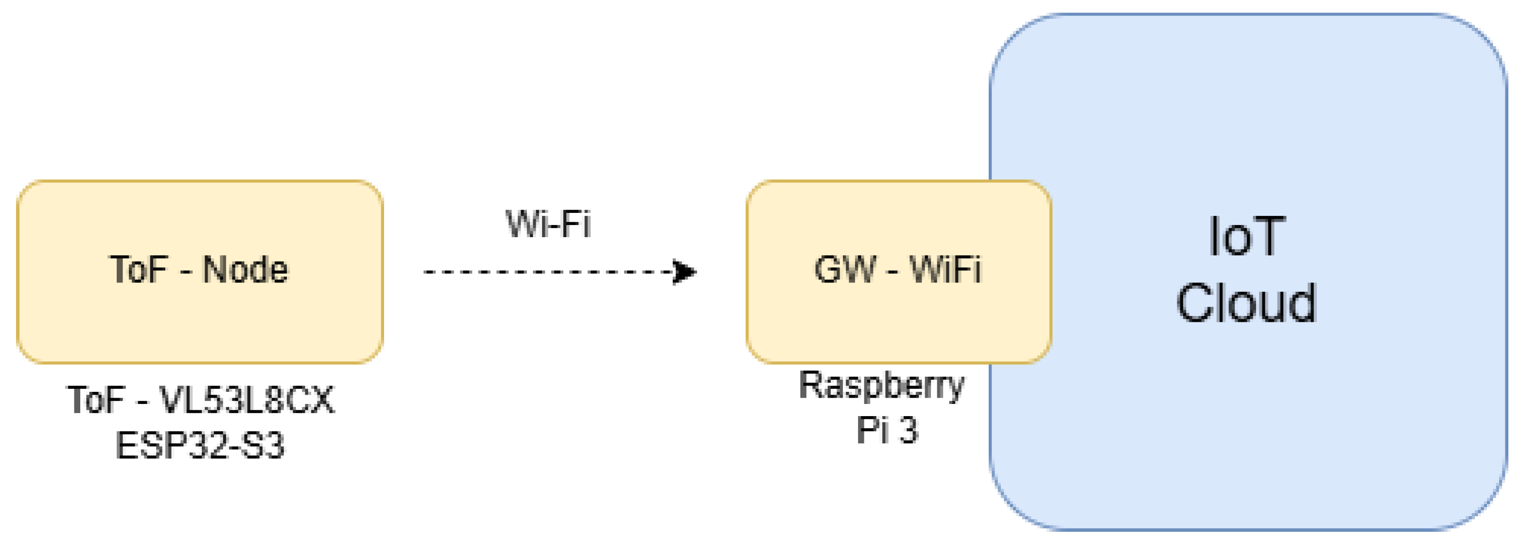
Figure 3 presents the system architecture for the experiment. System is composed of: ToF sensor – VL53L8CX [
17] and ESP32-S3 [
18], these two elements are the named ToF node, also included in the system Wi-Fi gateway based on Raspberry Pi3 – model B [
19] and a IoT Cloud [
20].
The VL53L8CX sensor, developed by STMicroelectronics [
17], is a distance measurement module that utilizes Time-of-Flight (ToF) technology, employing Continuous Wave (CW) modulation for high-precision distance measurements. This sensor is favored for its capability to measure distances across multiple zones concurrently and its durability in various environmental conditions. It incorporates a Vertical Cavity Surface Emitting Laser (VCSEL) that emits infrared light at a wavelength of 940 nm. This emitted light reflects off surrounding objects and returns to the sensor, where it is detected by an array of SPADs. The sensor calculates the time of flight of the light using CW modulation, which facilitates the measurement of the phase of the reflected light to ascertain distance. CW modulation allows the sensor to differentiate between various light paths (both direct and reflected), thereby minimizing errors induced by ambient light or multiple reflections. This technique enhances both accuracy and spatial resolution, enabling dependable measurements even in challenging environments.
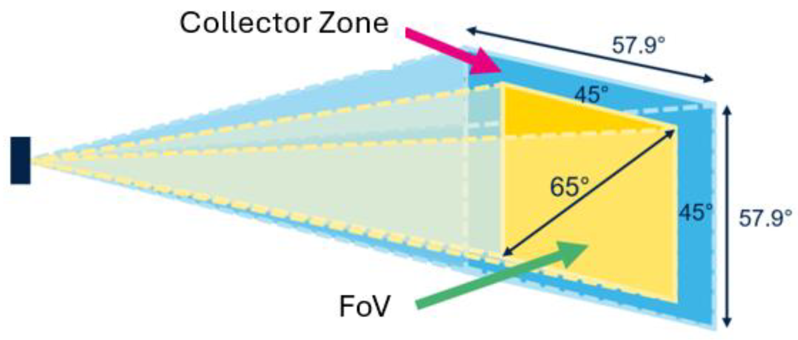
The VL53L8CX sensor features sophisticated processing capabilities to mitigate the effects of ambient light and interference. It supports multizone measurements, allowing for distance measurements in up to 64 simultaneous zones arranged in an 8x8 matrix, with adjustable spatial resolution ranging from 4x4 to 8x8 zones based on specific application needs. The sensor’s operational range extends up to 4 meters, contingent upon the object’s reflectivity, with a minimum measurable distance of 1 cm and an accuracy of ±1 cm. The Field of View (FoV) can be configured to a maximum of 63° x 63° (
Figure 4), and the update frequency can reach up to 60 Hz (for 8x8, frequency: 15 Hz and 4x4, frequency: 30 Hz). Communication with the microcontroller is facilitated via an I2C interface operating at a voltage of 3.3 V. The sensor’s dimensions are 4.4 mm x 2.4 mm x 1.9 mm.
In
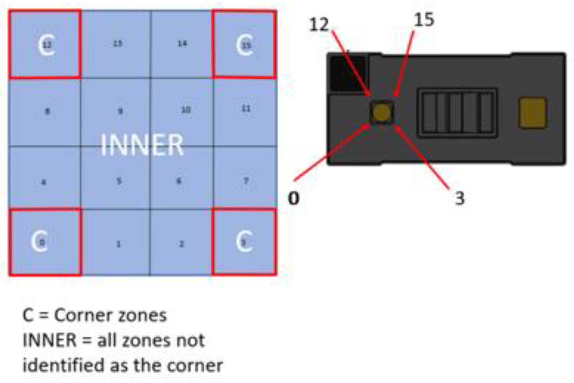
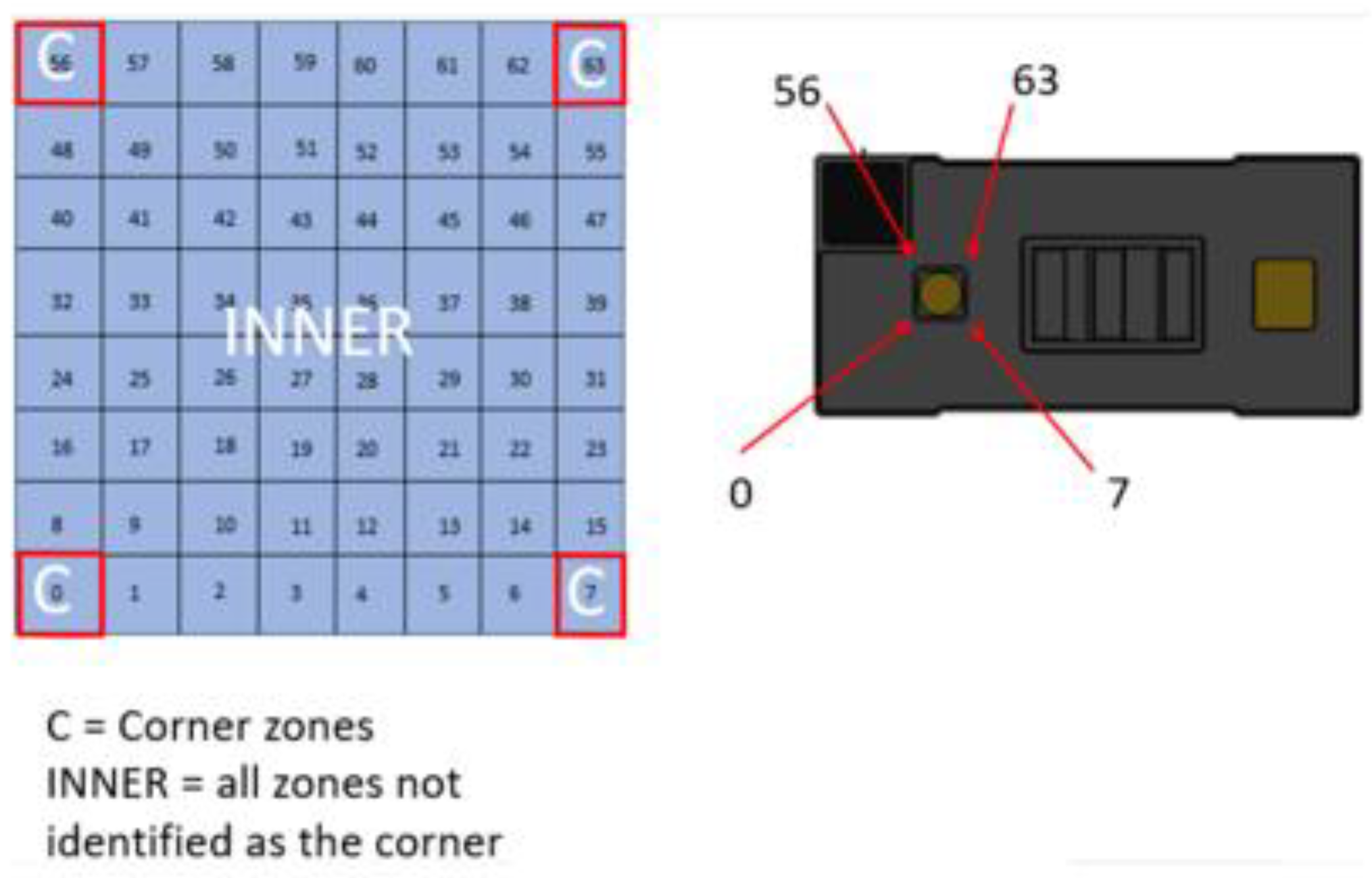
Figure 4, we have a 45° projection angle with a 65° diagonal FoV. There are potential problem (
Figure 5 and
Figure 6), the sensor has different resolutions as we know, and this is going to affect our values, for instance, the values of the corners are the most “unstabble”, being the inner ones the ones we want to work with, so, using the 4x4 resolution, we have around 12 points that we can work with, whilst the 8x8 resolution gives us 60 points.
When we combine this 2 topics (range and reflection) into a table to compare values (4x4 vc 8x8), we get a better understanding about what we are working with and possible problems that we might face. In [
9] it can be seen a table with: FoV, zone and ambiente ligth for the 8 x 8 resolution. We can now see the problems that we face once we step into long range readings, going from losing 5 centimeters to losing about 2050 centimeters (in the dark), and in the ambient light, the losses are almost 50%. And, of course we have tolerances, or better said, accuracy and what are the expected losses (assuming a perfect mounting of the set up).
The ESP32-S3 [
18] is a microcontroller with a dual-core processor running at up to 240 MHz, featuring an ultra-low-power RISC-V co-processor. It supports Wi-Fi (2.4 GHz) and Bluetooth 5 (including BLE and Mesh). The device includes 8 MB of internal flash, 8 MB of external PSRAM, 512 kB of SRAM, and 384 kB of ROM. It offers various power management features, USB functionalities (Native USB, Serial USB JTAG, USB OTG), and 27 GPIO pins with multiple peripheral interfaces (SPI, I2C, UART, I2S, ADC). Its compact size (23.5 mm x 18 mm) and integrated ceramic antenna make it ideal for space-constrained applications. In this setup, I2C pins are connected to a ToF sensor.
The Raspberry Pi 3 Model B [
19] is a single-board computer running Ubuntu Server 22.04.4 LTS on a 32 GB micro SDHC card. It features a 1.4 GHz Broadcom BCM2837B0 processor, 1 GB of LPDDR2 SDRAM, dual-band Wi-Fi (2.4 GHz and 5 GHz), Bluetooth 4.2, and Gigabit Ethernet via USB 2.0. The board includes a 40-pin GPIO header, HDMI port, four USB 2.0 ports, and CSI/DSI ports for camera and touchscreen interfaces. In this experiment, it acts as a gateway between the ToF-Node and the IoT cloud (Sensefinity cloud [
20]).
3.2. Test Scenarios
In this experiment, a hollow block was used to establish the basic reference height. This was crucial for the study as it provided an understanding of the initial depth at which we were working, serving as a useful starting point for analysis. Subsequently, a block was retained in the scenario to examine the effects of all the modifications under investigation.
This scenario was tested using the same blocks as a base (36 mm), with two additional blocks of 36 mm height placed on top of the original, central object. This setup aimed to observe the effect of adding structural elements on the measurements made by the sensor.
A more complex scenario involved combining multiple structure objects that were superimposed. This scenario focused on measuring heights in intricate ways finding exact locations of the holes and pinpointing high or low points. Factors such as color of the object, angle of slant, room lighting, and potential sensor errors were considered to enhance the accuracy and reliability of the measurements.
In the final scenario, the objective was to analyze the measurements taken based on a remote setup. Here the sensor collected data and transferred it to a cloud platform. The data processing from the sensor included dimensions of objects, depth measurements, hole locations, and surface variations. This data was processed and compared in a digitally designed environment to examine:
Dynamic analysis on these measurements once processed in the cloud to rapidly adapt, identify patterns, and draw conclusions.
Integration of the results with predictive models or algorithms within substructures, correlating factors with brightness.
3.3. Hardware Integration
Based on
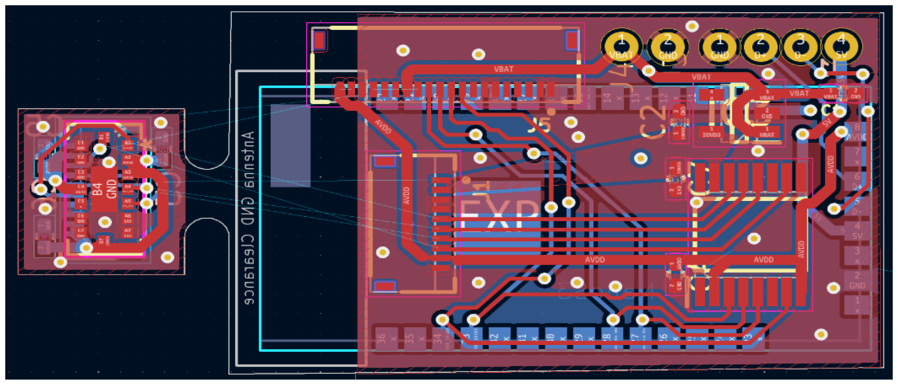
Figure 3, and for more facility during the experimental test, we design a schematic and after this a Printed Circuit Board (PCB) layout. In
Figure 7, it can be shown PCB layout that includes: ToF sensor and ESP32-S3. PCB has: 40 x 18 x 4 mm dimensions.
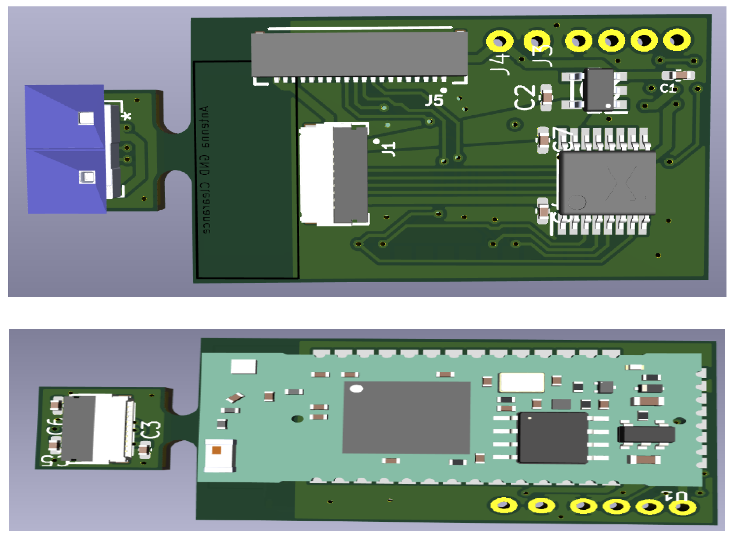
Figure 8 shows a 3D view (top and bottom).
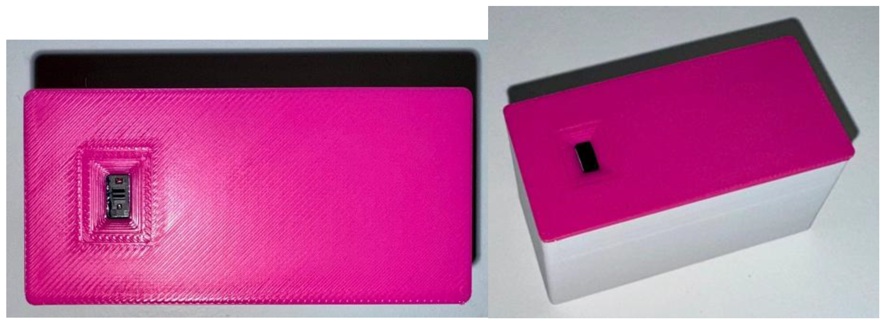
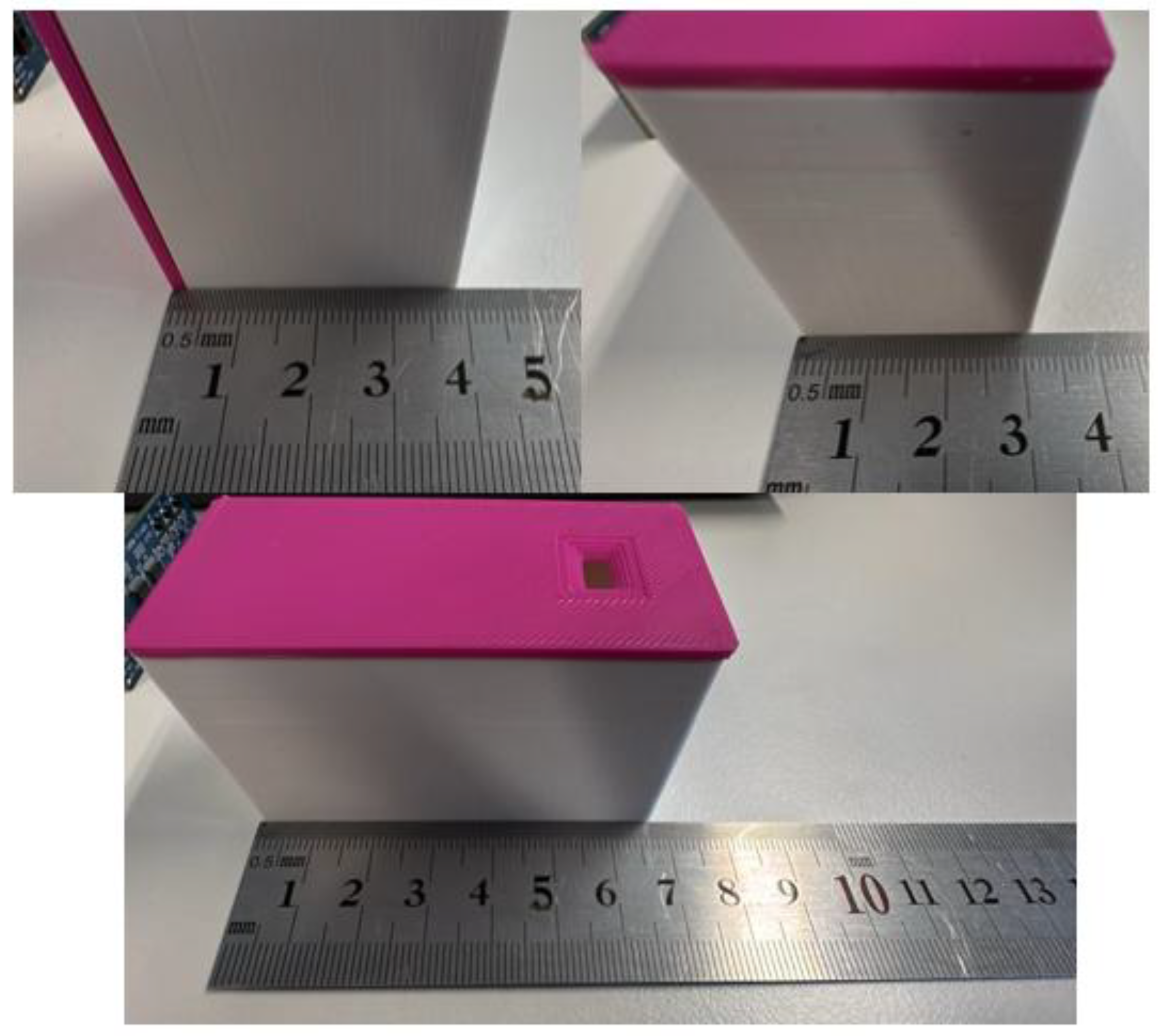
The final prototype for the experiment, with the components assembled inside a box and prepared for the use in the experiment,
Figure 9 and
Figure 10 (with dimensions).
3.4. Algorithms Developed
In ToF Node, a program is developed for ESP32-S3 board in C/C++, whose main function is to take the sensors reading and create a payload with these values to be sent to the Wi-Fi and show the values locally. The algorithm is shown in the next paragraph.
|
Algorithm: Integration of the ToF Node with Wi-Fi. |
1. System Setup
1.1. Initialize the I²C communication bus.
1.2. Initialize the wireless communication module (ESP32-S3).
1.3. Enable the power pin for the sensor, if available.
1.4. Configure the VL53L8CX sensor with the following parameters:
- Resolution: 8x8 zones, Set to VL53L8CX_RESOLUTION_8X8
- Metrics Enabled:
Signal Intensity (Signal): Disabled by default
Ambient Light (Ambient): Disabled by default
1.5. Start data acquisition from the sensor.
2. Main Operation Loop
While the system is running:
2.1. Check if new data is available from the sensor.
- If new data is ready:
a) Retrieve distance measurements for all 64 zones (8x8).
b) Retrieve additional metrics: signal intensity and ambient light.
c) Format the data for transmission.
d) Transmit the data to the remote device via Wi-Fi.
3. Data Display (only for monitoring ToF Node locally)
3.1. Organize and format measurement data.
3.2. Display the data by zones, including distance, signal intensity, and ambient light values. |
The Raspberry Pi was set up to connect to a Wi-Fi network, functioning as a gateway with cloud access. It was configured to operate as a Hypertext Transfer Protocol (HTTP) server, utilizing a Representational State Transfer (RESTful) API that facilitated communication with external devices. Through this API, the Raspberry Pi could receive data transmitted by the ESP32. Additionally, Raspberry Pi had internet access, which was essential for forwarding the received data to the cloud, thereby enabling communication between the local device (ESP32) and the remote cloud infrastructure.
The ESP32-S3 was also configured to connect to the same Wi-Fi network as the Raspberry Pi. It was programmed to gather local data, such as that from a ToF sensor, and to periodically transmit this data to Raspberry Pi over Wi-Fi. The transmission frequency was set so that the ESP32 would send information either at regular intervals or triggered by specific system events, such as sensor readings.
In this communication framework, the ESP32-S3 functioned as a Wi-Fi client, establishing a connection to the network already linked to the Raspberry Pi. The Raspberry Pi served as a server, awaiting connections from the ESP32-S3. To transmit data, the ESP32-S3 employed HTTP requests, leveraging a RESTful API for interaction with the Raspberry Pi. The data was sent via a GET request, with the information included as parameters in the request Uniform Resource Locator (URL). This method of GET request allowed for the efficient transmission of small data volumes, utilizing the URL to convey information as parameters.
Upon receipt of the data, the Raspberry Pi undertook the processing of the information. This process involved converting the received data into an appropriate format, such as JSON, to ensure ease of manipulation and compatibility with cloud systems. Once the data was processed, it was prepared for transmission to the cloud.
The data was sent to the cloud using the HTTPs protocol, which ensured the security of the data transmission. The Raspberry Pi initiated HTTPs requests to a RESTful API hosted in the Sensefinity cloud [
20].
4. Results
This section may be divided by subheadings. Firstly, apply ToF Node in different scenarios (with augmented complexity) and a cloud scenario. In section 4.3, we write about the energy consumption of the ToF Node.
4.1. Experiment Scenarios
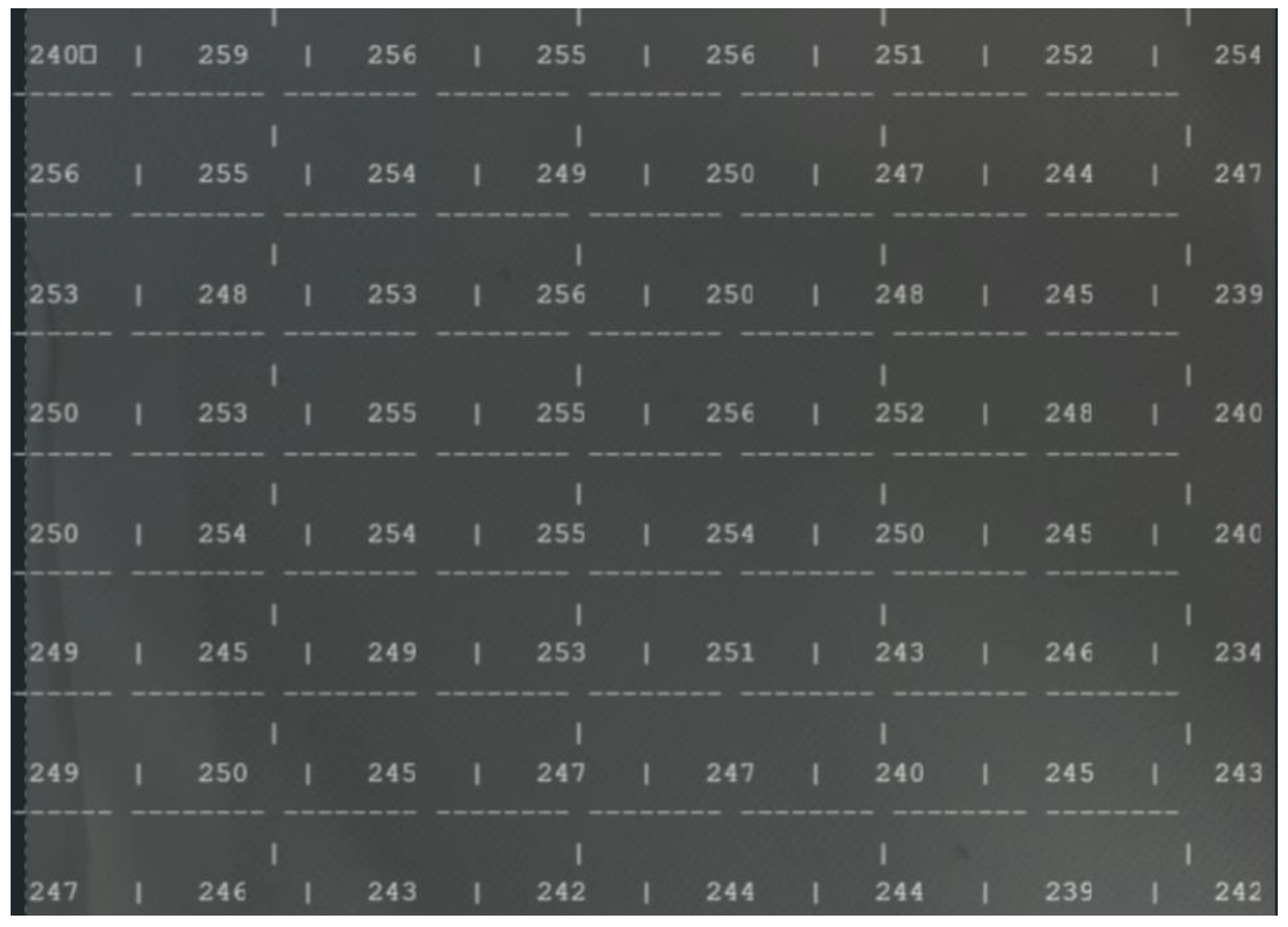
The following paragraphs explain the two first scenarios defined for the experiment, where the ToF-Node was at a height of 25 cm. All of the results presented in this section show that the matrix functions as a “depth map” of the scene in front of the sensor, with the numbers in the cells representing distances in millimeters; the 8x8 format indicates that the sensor is taking multiple measurements in a two-dimensional matrix, where the differences in values reflect the variation in depth, with smaller values indicating proximity and larger values representing longer distances.
-
- ◦
This experiment involves using the ToF sensor to measure the height of objects. It sets the foundation for understanding the sensor’s capabilities and accuracy.
- 2.
-
- ◦
In this scenario, a block is introduced to the setup. The goal is to observe how the sensor’s measurements are affected by the added structure.
- 3.
-
These scenarios collectively will provide a comprehensive understanding of the ToF sensor’s performance in various conditions and setups.
In the next sections we will provide the metrics of each block achieved with the help of the caliper.
Figure 12 presents the “view” of the ToF sensor.
4.1.1. Scenario: Measuring Height with ToF Sensor
In this experiment (
Figure 11), we have an empty photography block to understand the main height we will work with during this process. We will then add a block to observe its effect. The study follows this structure: description, demonstration of the physical scenario, and overlay of the scenario with the values of the results.
Initial Setup:
Analysing, the results shown in
Figure 12, is possible to observe an average of 250 mm (the ToF sensor measures in mm), that is, 25 cm from the top to the base of the office trash box, shown at the beginning (
Figure 11).
4.1.2. Adding a Block
Block Dimensions: A block with a height of approximately 25 mm is added to the base block of 52 mm inside the office trash box (
Figure 13). This block is smaller than the base block.
-
- ◦
-
Practical Measurement (base of the block): 250 mm- 202 mm = 48 mm
- ■
Difference: 52-48 mm= 4 mm
- ◦
-
Practical Measurement (Top of block): 250 mm - 176 mm = 74 mm
- ■
Difference: 77 (52+25)mm - 74 mm (real) = 3 mm
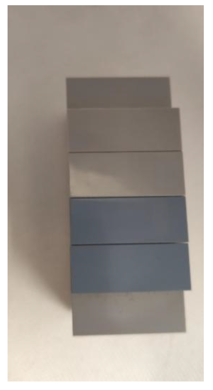
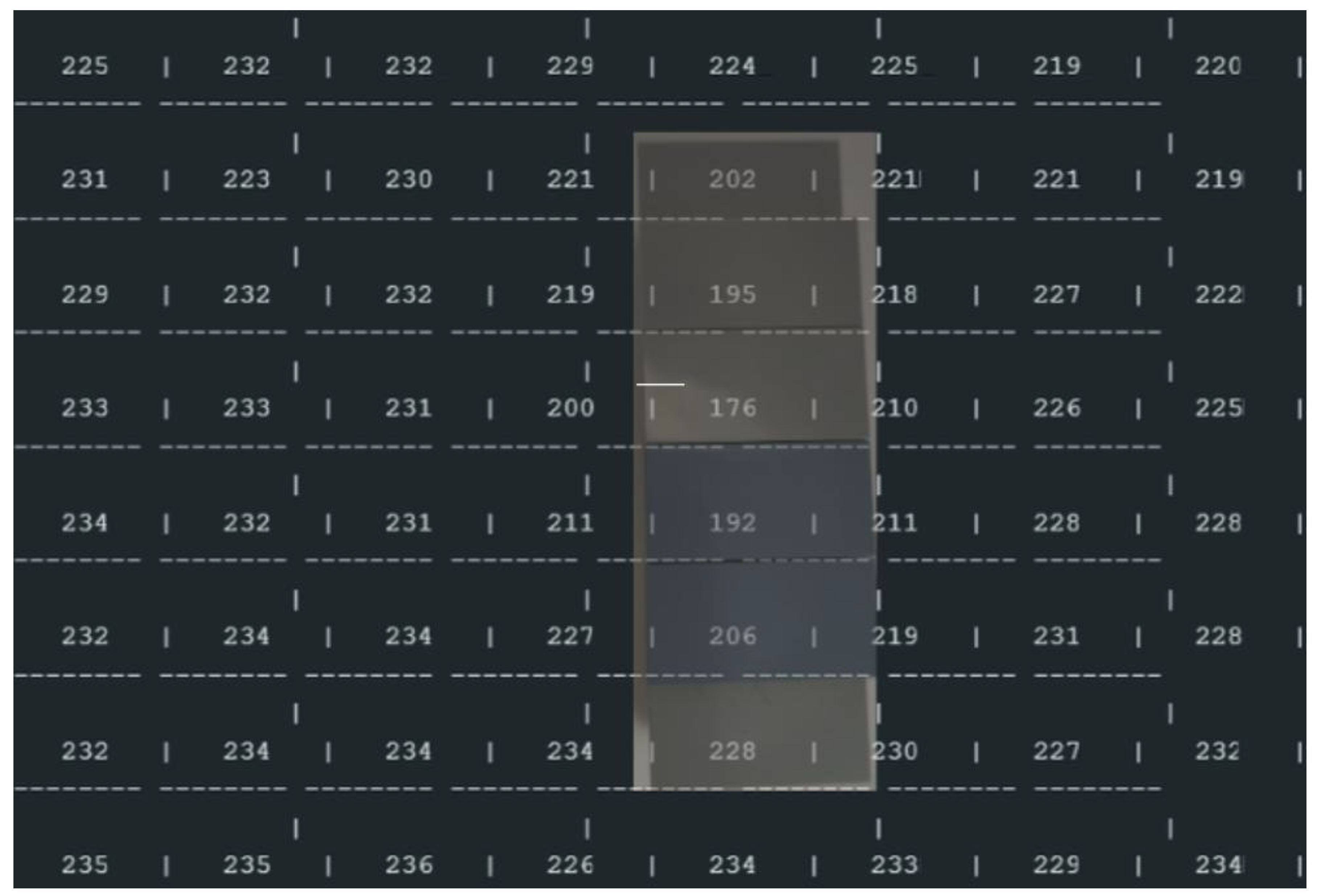
4.1.3. New Block Dimensions (two different blocks-Figure 15)
- ◦
Base to Top of Object: 36 mm
- ◦
Base to Hole: 20 mm
-
- ◦
-
Base to Top of Object: 250 mm−216 mm=34 mm
- ■
Difference: 36-34 mm= 2 mm
- ◦
-
Base to Hole: 250 mm−229 mm=21 mm
- ■
Difference: 20-21 mm= -1 mm
In order to evaluate and analyze the data collected, it was created a table (
Table 2) that sumarize the results. Note that:
Negative Measurements: Indicate the sensor perceives the object as lower than it actually is.
Positive Measurements: Indicate the sensor perceives the object as higher than it actually is.
Value 0: Does not exist in the measurements.
Reflections can sometimes cause discrepancies in measurements. However, these reflections generally do not significantly impact the overall precision of the system. Additionally, this system is not intended for use in garbage cans containing glass or metal, which helps mitigate potential issues from reflections.
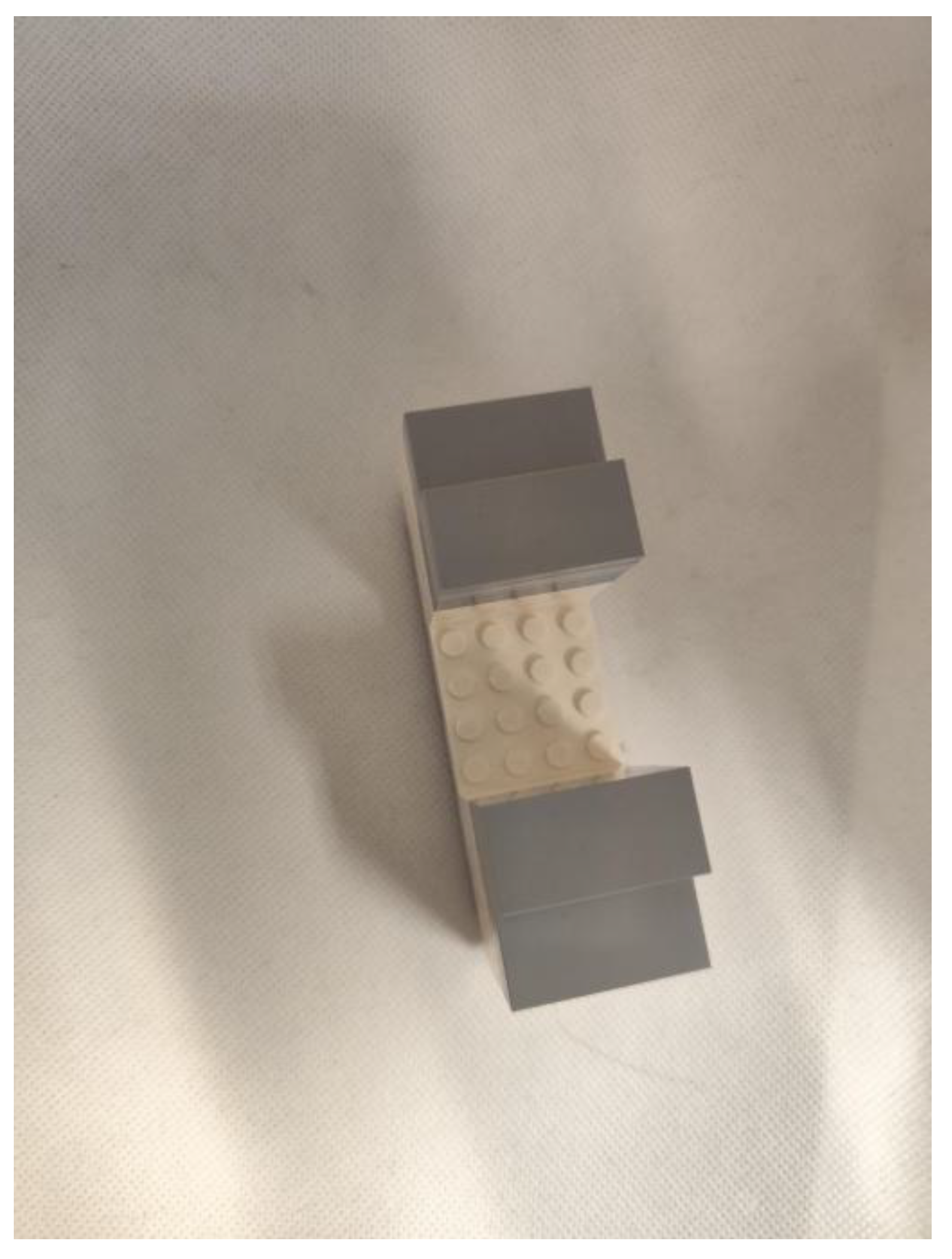
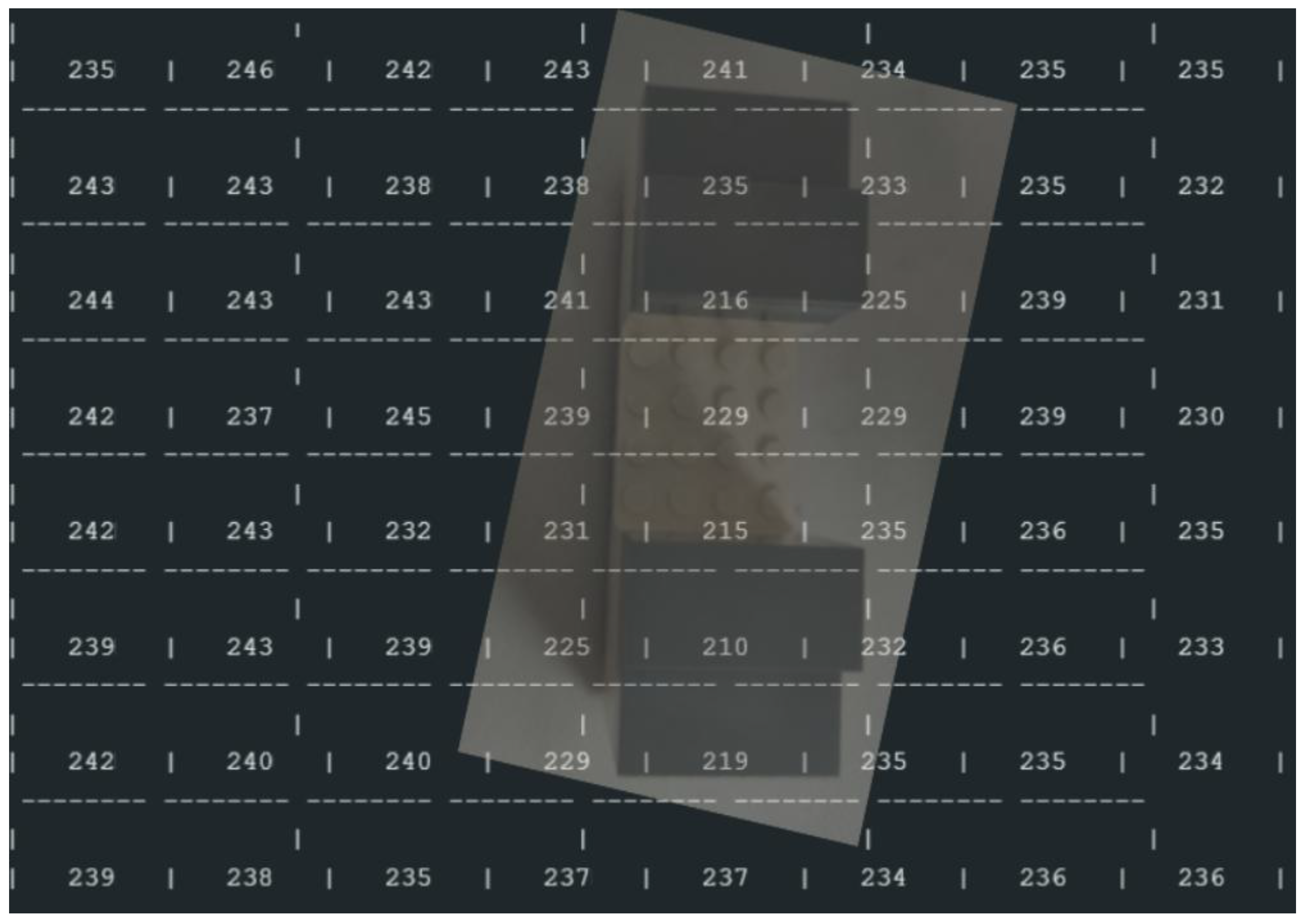
4.2. Scenario in a Closed Box
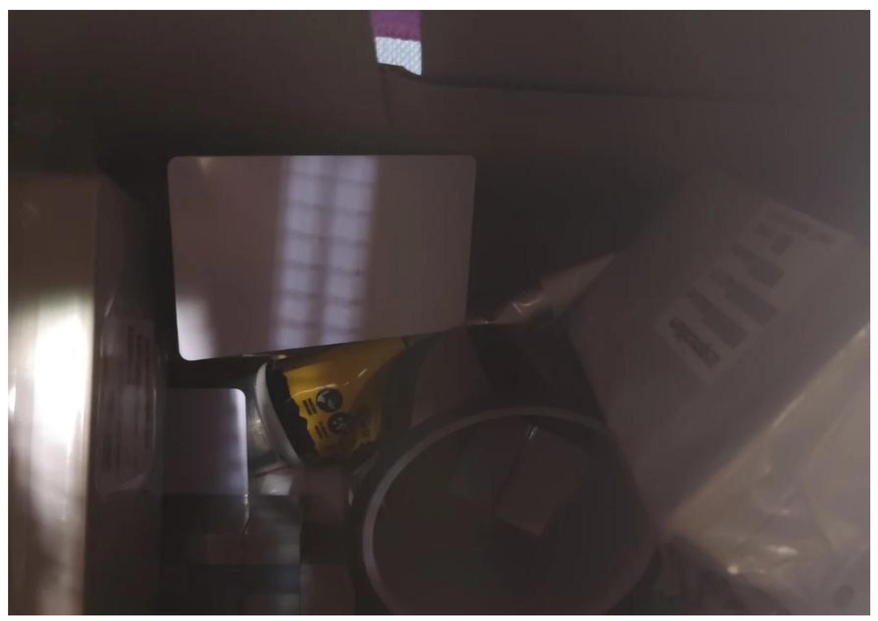
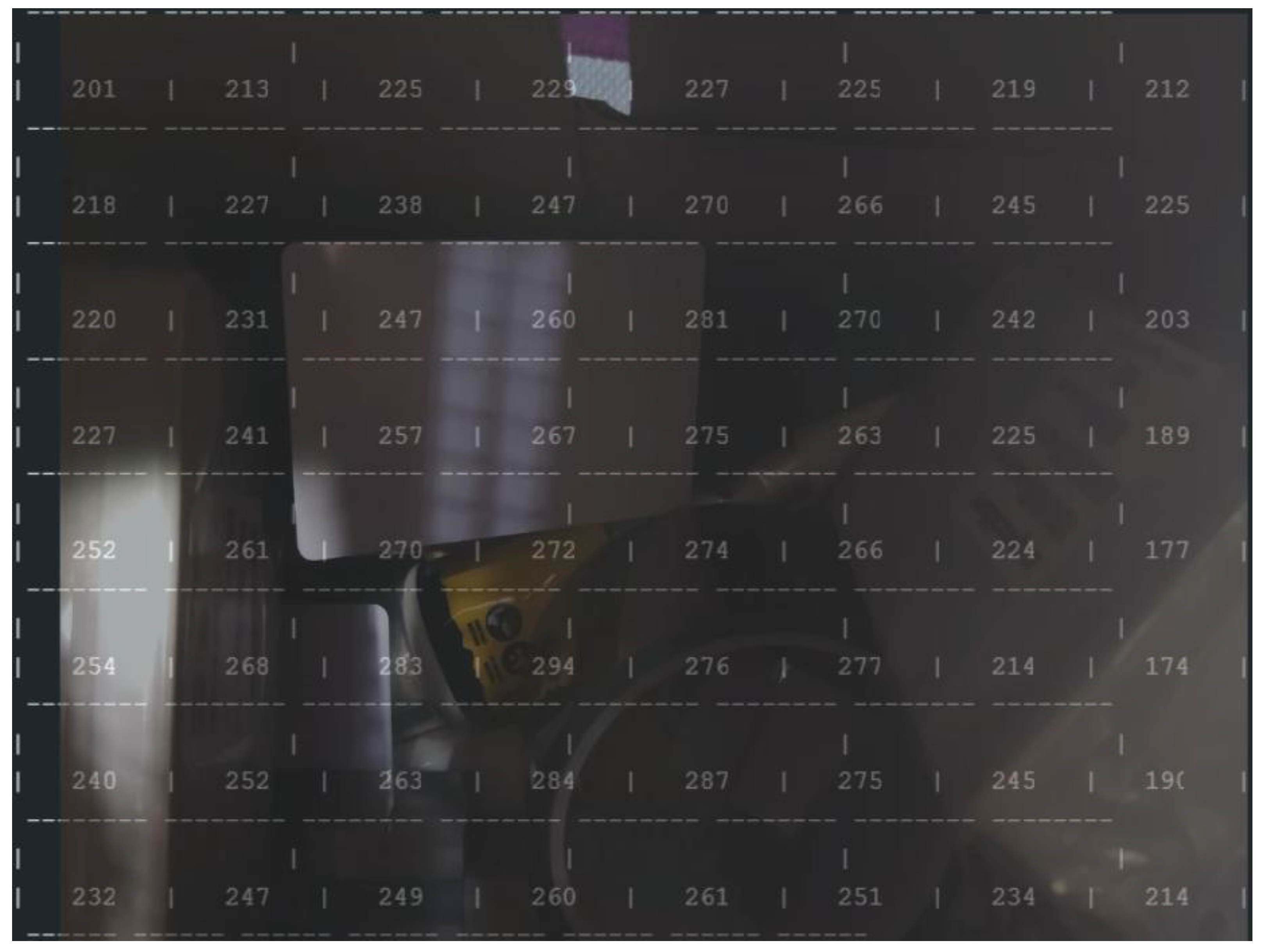
In this scenario (
Figure 17), multiple objects were stacked inside a closed box to simulate a confined environment and ToF-Node stands at a height of 25 cm. This setup allows for detecting the relative quantity of trash in a trash can, for example, testing the sensor’s ability to detect and analyze objects in a restricted space. It helps perceive inclinations and various possible reliefs through the values received, despite the irregular angles of the objects preventing exact measurements. The results are presented in
Figure 18.
The maximum values recorded are 294 mm (approximately 0.29 meters). The objects are closer to the sensor (200 to 300 mm) and closer together. (4) The arrangement of the values suggests that the sensor is measuring an uneven surface or an object with depth variations.
4.3. Cloud Scenario
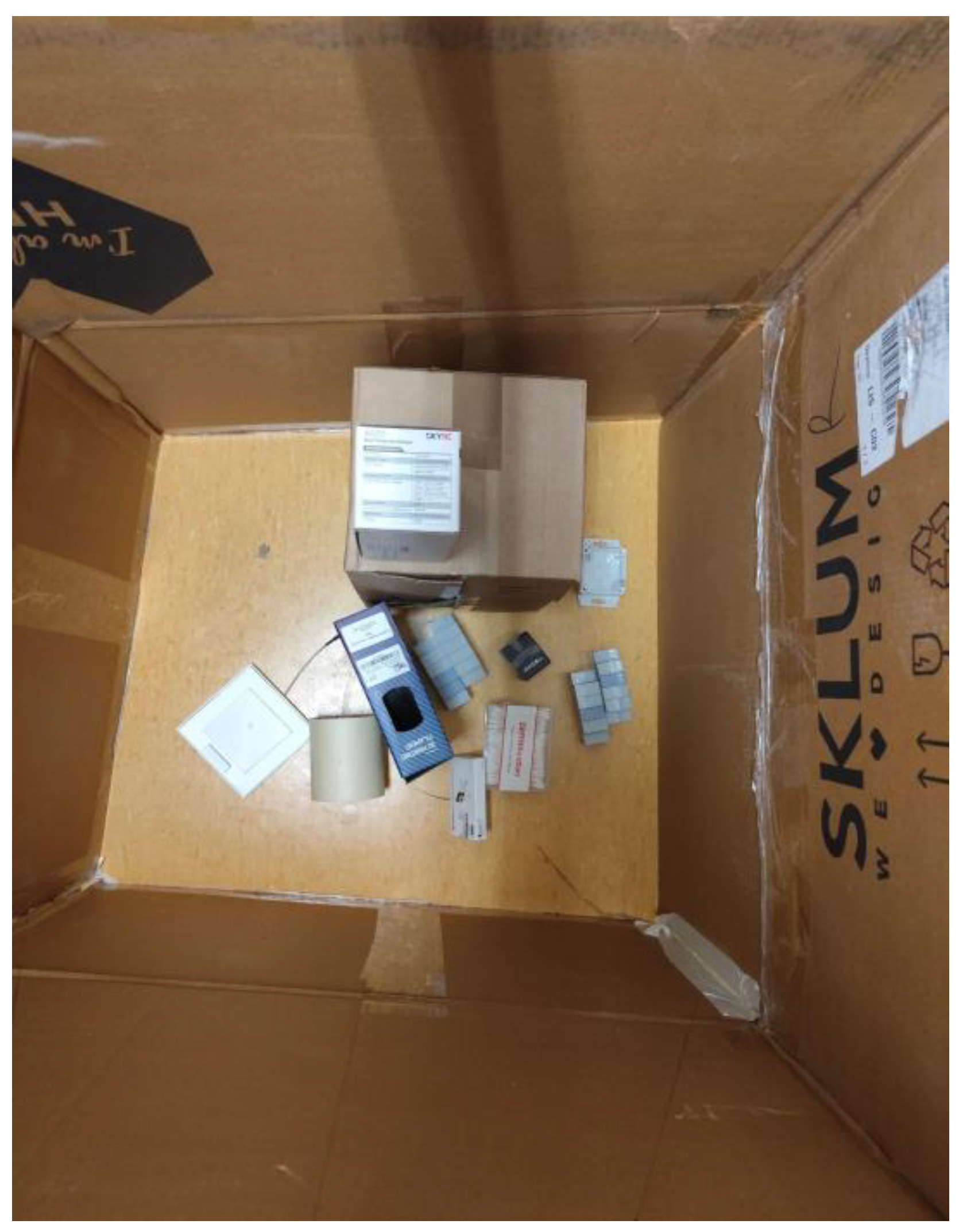
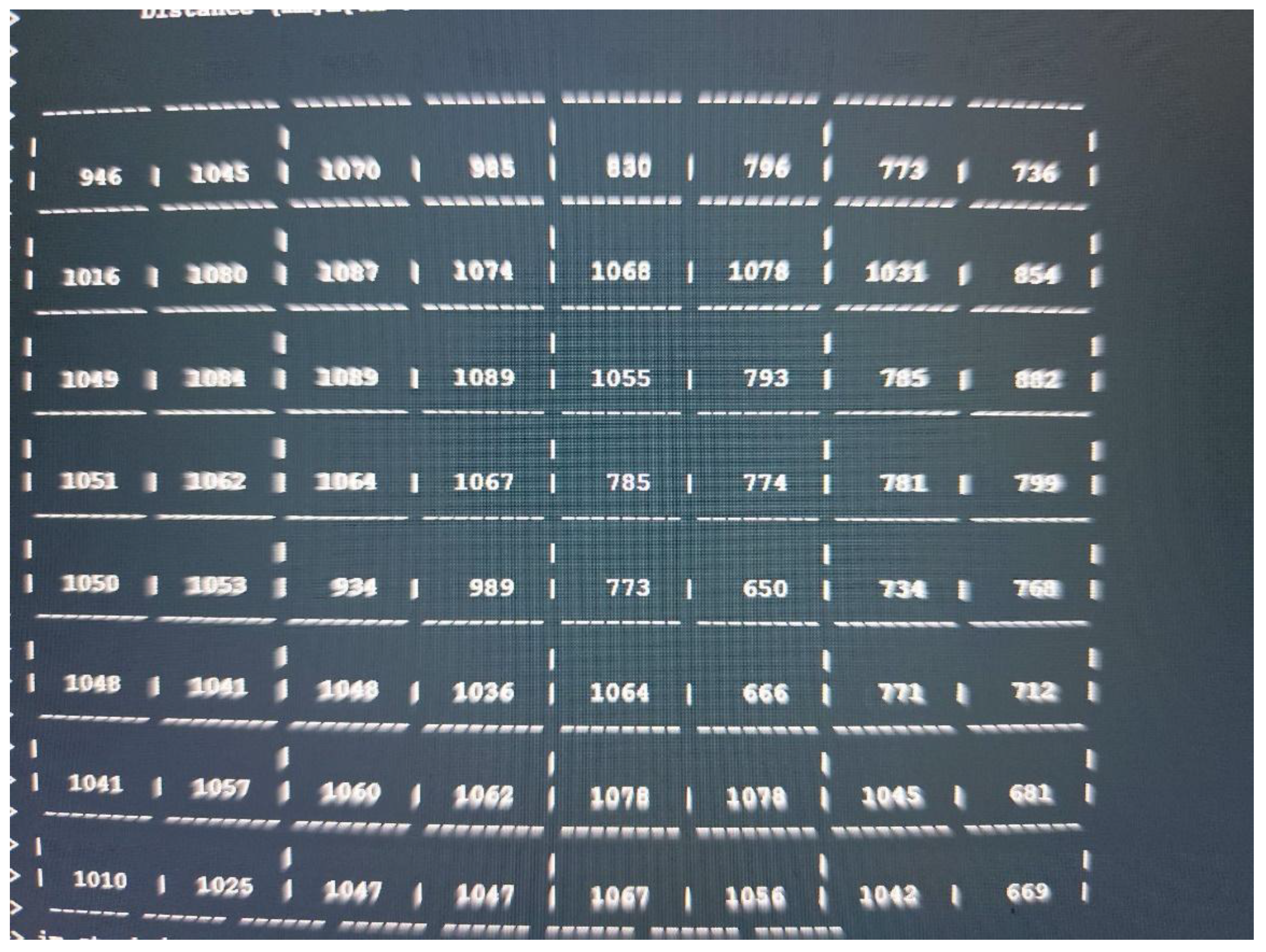
Finally, we try another experience to send data collected to IoT cloud. In
Figure 19, we present the trash inside the box with the biggest box. The ToF-Node stands at a height of 110 cm.
Smaller values (e.g., 650, 666, 681 mm) indicate the presence of a closer object in the area. The larger values (e.g., 1089, 1078, 1068 mm) represent more distant areas or flat surfaces. The arrangement of the values suggests that the sensor is measuring an uneven surface or an object with depth variations. The maximum values recorded in the 8x8 matrix were in the order of 1089 mm (approximately 1.09 meters). There was significant variation between different areas of the matrix.
In
Figure 21, we presente the data send to IoT gateway (RP3)
The API of Sensefinity IoT cloud, lets us access an IP address, and, through a certain “door”, we can access the values that we wish. It was also added the reliability of the values in a scale from 0 to 5, this makes us able to know if it is a good idea to use that value, or if that value is reliable for measurements or decisions to be made according to those same values. For instances, if the value has a reliability of “5”, then it means that it is a strong value, a strong signal that we can count with, while if it goes down to a 2, it means that the value might be inconsistent and that we shouldn’t really trust it. Once we introduce the IP address followed by the gate, (eg: xxx.xxx.x.xxx : yyyy) we get what the API is sending or representing,
Figure 22.
This is due to a possible idea and implementation of the API, we tend to use this in order to have a 3D representation through Sensefinity’s Cloud processment capability to get an idea of the container inside objects positions and heights (
Figure 23,
Figure 24,
Figure 25,
Figure 26). For exemple, with this API, we are able to export the data via Wi-Fi and get the 3D rendering of the values in the clouds storage, making us able to monitor the space.
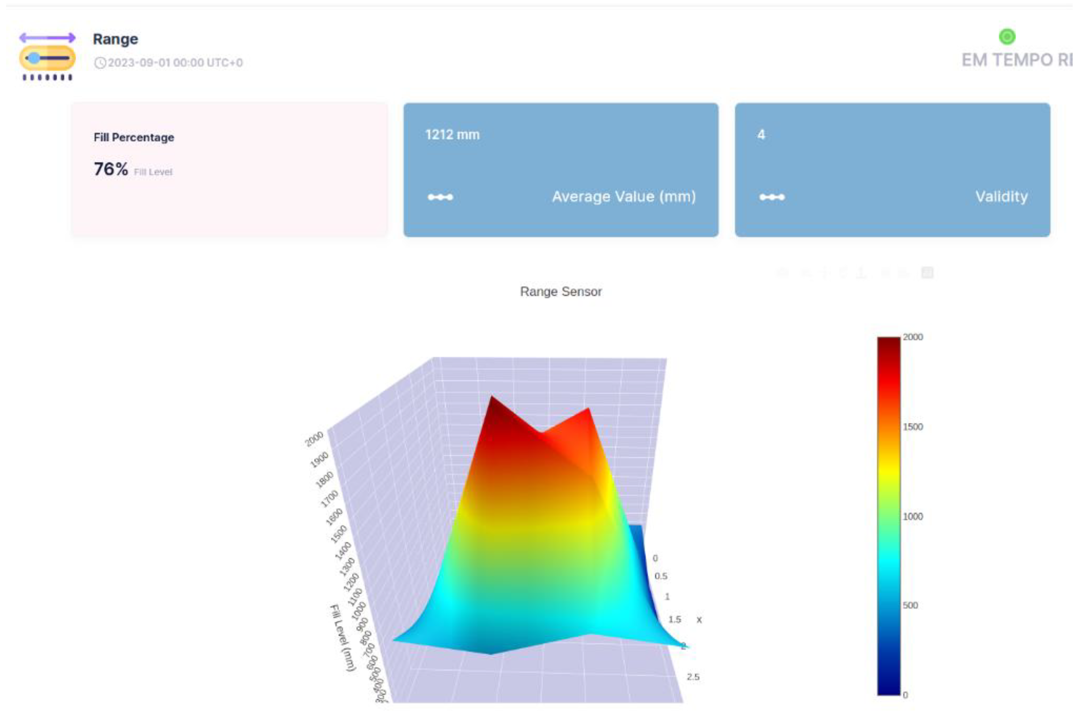
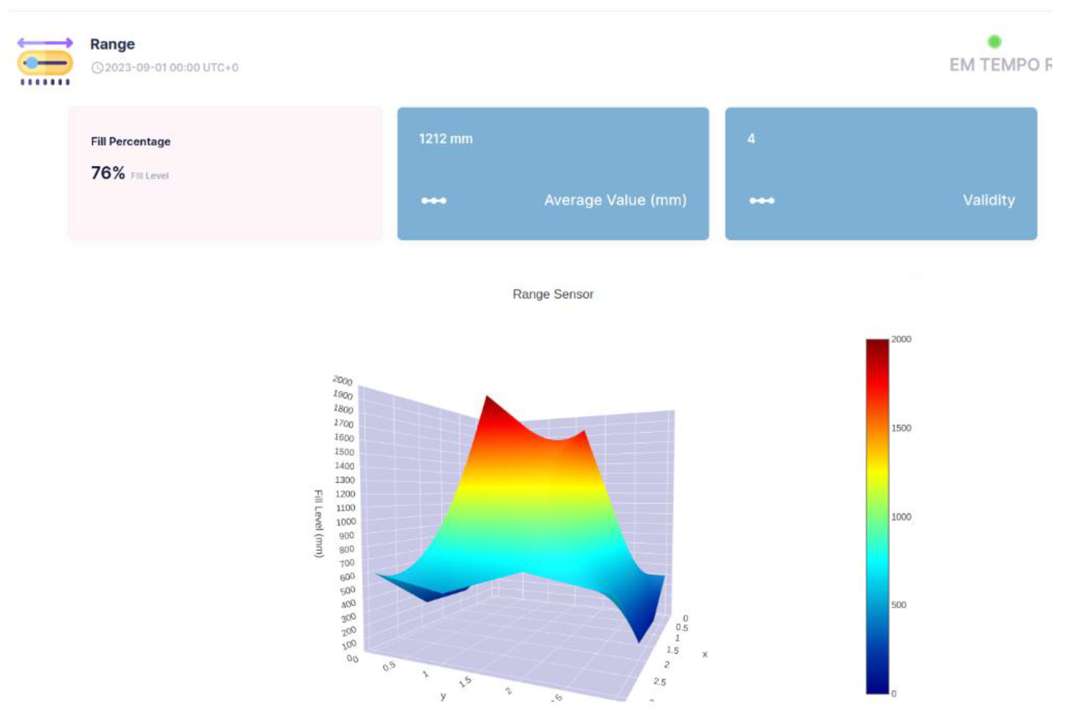
In Figures 23 to 26, the interface belongs to Sensefinity and displays data related to the volumetry of a tank or container.
Interface elements:
Fill (%) - Indicates an occupancy level of 76 %, referring to the fraction of the container’s total volume.
Average Value (mm) - The average of the measurements taken by the sensor is 1212 mm.
Validity - An indicator of data quality, in this case represented by the value 4.
3D Graph - Volumetric representation of the sensor data, showing a colored surface with a depth scale. The coloring varies from blue (low level) to red (high level), making it possible to visualize irregularities on the surface of the measured material.
Real-time update - The interface displays the information with continuous updates to allow dynamic monitoring of the values.
For example in
Figure 24, highlight in the 3D Graph - The volumetric graph now displays a specific point with the coordinates: X: 2; Y: 2; Z: 1500 mm
This represents a point in three-dimensional space where the sensor has measured a depth of 1500 mm.
Improved Visualization - The inclusion of black lines in the graph improves the segmentation and interpretation of the depth data.
Rest of Interface - The values displayed remain the same: 76% fill, 1212 mm average value and Validity of 4.
This type of detailed visualization helps to identify patterns, variations in the volumetry of the measured material, IoT applications that require volumetric monitoring, such as tank, silo or waste container management, enabling logistics optimization and decision-making based on real-time data.
4.3. Energy consumption
The VL53L8CX time-of-flight sensor and ESP32-S3 microcontroller communicate in different power consumption modes to maximize battery life. The VL53L8CX requires 10 mA in active mode and only 55 µA in low-power mode. The ESP32-S3 consumes 45 mA when not using Wi-Fi, 120 mA while transmitting data over Wi-Fi, and can achieve deep sleep with a current draw of just 100 µA.
Data transmission is split into two stages: 30 ms for communication from the ESP32-S3 to the gateway and 200 ms for the gateway to the cloud. One data acquisition cycle lasts 15 ms per frame, with each frame consisting of depth data measurements from 64 points to either rebuild the depth image or analyze the environment. The Joulescope was used to measure consumption accurately.
Every 3600 seconds, measuring and sending data consumes 130 mA for 45 ms (15 ms measurement + 30 ms Wi-Fi transmission), resulting in an energy expenditure of 5.85 mAh. During the remaining 3599.955 seconds, the system is in low-power mode, consuming 0.558 mAh, given by the combined consumption of the ESP32-S3 and ToF sensor at 155 µA.
Repeating this measuring and sending cycle every 3600 seconds results in 24 cycles per day, leading to a total daily consumption of approximately 153.8 mAh. Considering a 3.6V, 3350 mAh Li-Ion 18650 battery (LG INR18650 model), the system’s estimated autonomy is around 22 days
5. Conclusions
This study presents an integrated approach resulting in a prototype that offers a reliable and affordable solution for real-time monitoring of garbage levels using volumetric ToF sensors. Initially, the system was designed to connect to a Wi-Fi network, with the Raspberry Pi functioning as a gateway with cloud access and the ESP32-S3 gathering local data. The data was transmitted securely to the cloud using the HTTPs protocol, enabling efficient communication between the local device and the remote cloud infrastructure.
The findings are quite promising, as laboratory tests demonstrated a higher level of precision than would be necessary in real-world conditions. This suggests that the system is robust and effective even under less controlled environments. The decision to incorporate the ToF-Node has proven advantageous, enhancing usability and confirming its low power consumption, which underscores its portability.
The three-dimensional visualization of volume and level on the cloud IoT dashboard has demonstrated significant advantages, facilitating the prospective incorporation of additional ToF sensors. This advancement will reduce the importance of sensor placement within waste containers. Additionally, the reliability scale integrated into the API aids in evaluating the credibility of the data, ensuring that only precise and consistent information is utilized for essential decision-making. In the future, there is potential for data storage on a blockchain, such as an elastic blockchain platform, which would enable the monitoring of waste collection and delivery routes. This capability would support cloud-based tracking of the permanent location of waste collection vehicles, achievable through the straightforward integration of a geolocator and communication with the cloud.
The system proposed has several advantages:
Cost-Effectiveness: Utilizing affordable components like the ToF sensor and ESP32-S3 makes this solution accessible for various applications without significant financial investment. The total cost would be 22€.
Scalability: The system can be easily scaled by adding more sensors or devices, allowing for extensive monitoring and data collection.
Flexibility: The use of a RESTful API and HTTPs protocol ensures compatibility with various cloud platforms and services, providing flexibility in data handling and processing.
Real-Time Monitoring: The integration in a IoT cloud enables real-time data visualization and analysis, facilitating prompt decision-making.
Reliability: The reliability scale implemented in the API helps in assessing the trustworthiness of the data, ensuring that only accurate and consistent values are used for critical decisions.
Portability: The low power consumption of the ToF-Node highlights its complete portability, making it suitable for various environments and applications.
Compact Design: The small size of the ToF-Node (40 x 18 x 4 mm PCB) and its enclosure (65 x 40 x 30 mm) make it easy to deploy in various urban environments.
The ToF sensor’s high precision revealed itself to be essential for accurately measuring and detecting variations in object dimensions and positions. This ensures reliable data collection and analysis, which is fundamental for real-time monitoring and decision-making processes. In this experiment, the objects modeled a trash bin, demonstrating the sensor’s ability to detect the fill level, identify irregularities, and monitor the overall status of the bin. This capability enhances the system’s effectiveness in various environments, making it suitable for applications such as waste management, inventory control, and environmental monitoring.
Overall, this solution provides a comprehensive, reliable, and scalable approach to monitoring and data transmission, making it suitable for a wide range of applications that can be applied, particularly in the context of smart cities. The successful integration of ToF sensors in a connected device ecosystem, along with the effective use of cloud services, demonstrates its potential to enhance real-time monitoring and decision-making processes. Additionally, the system can be integrated into a multi-parameter monitoring setup, where not only fill levels but also humidity, temperature, and harmful gases can be monitored. This would be object of analysys in a future work. Conversely, it will be important to consider the management of various ToF-Nodes at the gateway level in the future, as well as conducting tests outside of laboratory settings, specifically in waste containers utilized in public residential areas.
Acknowledgments
The authors would like to express their gratitude to Sensefinity company for making the sensor used during the experiments, as well as the use of the Sensefinity IoT cloud.
Conflicts of Interest
The authors declare no conflicts of interest.
References
- United Nations, “Sustainable Development Goals (SDGs)”, 2023. Available online: https://sdgs.un.org/goals (accessed on 5 January 2025).
- European Commission, “Circular Economy Package”, 2015. Available online: https://ec.europa.eu/environment/circular-economy/ (accessed on 5 January 2025).
- European Commission, “Strategy for plastics in the circular economy”, 2018. Available online: https://ec.europa.eu/environment/waste/plastic_waste.htm (accessed on 5 January 2025).
- European Commission, “Strategy for the Circular Economy”, 2020. Available online: https://ec.europa.eu/environment/circular-economy/ (accessed on 5 January 2025).
- May, S.; Droeschel, D.; Holz, D.; Fuchs, S.; Malis, E.; Nüchter, A.; Hertzberg, J. Three-dimensional mapping with time-of-flight cameras. Journal of Field Robotics 2009, 26, 934–965. [Google Scholar]
- Niclas, C.; Favi, C.; Kluter, T.; Monnier, F.; Charbon, E. Single-Photon Synchronous Detection. IEEE Journal of Solid-State Circuits 2009, 44, 1977–1989. [Google Scholar]
- Foix, S.; Alenyà, G.; Torras, C. Lock-in Time-of-Flight (ToF) Cameras: A Survey. IEEE Sensors Journal 2011, 11, 1917–1926. [Google Scholar]
- Xuming Luan. Experimental investigation of photonic mixer device and development of TOF 3D ranging systems based on PMD technology. Diss., Department of Electrical Engineering and Computer Science, University of Siegen 2001.
- Larry, Li. Time-of-Flight Camera - An Introduction. Texas Instruments - Technical White Paper, 2014.
- Lange, R.; Seitz, P. Solid-State Time-of-Flight Range Camera. IEEE Journal of Quantum Electronics 2001, 37, 390–397. [Google Scholar]
- Miles Hansard, Seungkyu Lee, Ouk Choi and Radu Horaud. Time of Flight Cameras: Principles, Methods, and Applications. Springer, 2012. ISBN: 978-1-4471-4658-2.
- M. A. A. Mamun, M. A. Hannan, A. Hussain and H. Basri, “Wireless Sensor Network Prototype for Solid Waste Bin Monitoring with Energy Efficient Sensing Algorithm,” 2013 IEEE 16th International Conference on Computational Science and Engineering, Sydney, NSW, Australia, 2013, pp. 382–387. [CrossRef]
- P. Reis, R. Pitarma, C. Gonçalves and F. Caetano, “Intelligent system for valorizing solid urban waste,” 2014 9th Iberian Conference on Information Systems and Technologies (CISTI), Barcelona, Spain, 2014, pp. 1–4. [CrossRef]
- S. Lokuliyana, A. Jayakody, G. S. B. Dabarera, R. K. R. Ranaweera, P. G. D. M. Perera and P. A. D. V. R. Panangala, “Location Based Garbage Management System with IoT for Smart City,” 2018 13th International Conference on Computer Science & Education (ICCSE), Colombo, Sri Lanka, 2018, pp. 1–5. [CrossRef]
- S.Satyamanikanta, N. Madeshan, Smart garbage monitoring system using sensors with RFID over internet of things. Journal of Advanced Research in Dynamical and Control Systems. 9. 6-2017.
- Zhang, Y.; Chen, J.; Wang, Q. Time-of-Flight Sensors vs. LiDAR: A Comparative Study for Indoor Mapping Applications. MDPI Sensors 2022, 22, 1051. [Google Scholar] [CrossRef]
- STMicroelectronics, “VL53L8CX”, [Online]. Available online: https://www.st.com/en/imaging-and-photonics-solutions/vl53l8cx.html. (accessed on 22 January 2025).
- Espressif Systems, “ESP32-S3”, [Online]. Available online: https://www.espressif.com/en/products/socs/esp32-s3. (accessed on 22 January 2025).
- Raspberry Pi, “Raspbery Pi 3 - model B”, [Online]. Available online: https://www.raspberrypi.com/products/raspberry-pi-3-model-b/ (accessed on 22 January 2025).
- Sensefinity, [Online]. Available online: https://www.sensefinity.com/ (accessed on 22 January 2025).
Figure 1.
Pulsed ToF method: The received signal is sampled in two out-of-phase windows in parallel (adapted from [
9]).
Figure 1.
Pulsed ToF method: The received signal is sampled in two out-of-phase windows in parallel (adapted from [
9]).
Figure 2.
Demodulation principle of CW method: C1 to C4 are control signals with 90° phase delay from each other (adapted from [
9] [
11]).
Figure 2.
Demodulation principle of CW method: C1 to C4 are control signals with 90° phase delay from each other (adapted from [
9] [
11]).
Figure 3.
System architecture.
Figure 3.
System architecture.
Figure 4.
Projection angle and diagonal FoV (adapted from [
9]).
Figure 4.
Projection angle and diagonal FoV (adapted from [
9]).
Figure 5.
ToF sensor for 4x4 resolution (adapted from [
9]).
Figure 5.
ToF sensor for 4x4 resolution (adapted from [
9]).
Figure 6.
ToF sensor for 8x8 resolution (adapted from [
9]).
Figure 6.
ToF sensor for 8x8 resolution (adapted from [
9]).
Figure 7.
PCB layout of ToF Node: ToF sensor and ESP32-S3.
Figure 7.
PCB layout of ToF Node: ToF sensor and ESP32-S3.
Figure 8.
ToF Node 3D view: PCB with ToF sensor and ESP32-S3.
Figure 8.
ToF Node 3D view: PCB with ToF sensor and ESP32-S3.
Figure 9.
Final prototype (ToF Node) for use in the experiment.
Figure 9.
Final prototype (ToF Node) for use in the experiment.
Figure 10.
Final prototype (ToF Node), with dimensions.
Figure 10.
Final prototype (ToF Node), with dimensions.
Figure 11.
Office trash box – main “scene” for tests (perfil view).
Figure 11.
Office trash box – main “scene” for tests (perfil view).
Figure 12.
Results of the ToF sensor with empty office trash box.
Figure 12.
Results of the ToF sensor with empty office trash box.
Figure 13.
Fisrt block add inside the office trash box.
Figure 13.
Fisrt block add inside the office trash box.
Figure 14.
Results of the ToF sensor with the first block inside the office trash box (superposed images).
Figure 14.
Results of the ToF sensor with the first block inside the office trash box (superposed images).
Figure 15.
Add the second block (with new block dimensions) inside the office trash box.
Figure 15.
Add the second block (with new block dimensions) inside the office trash box.
Figure 16.
Results of the ToF sensor with the new dimensions block inside the office trash box.
Figure 16.
Results of the ToF sensor with the new dimensions block inside the office trash box.
Figure 17.
Different kind of blocks in the inside the office trash box.
Figure 17.
Different kind of blocks in the inside the office trash box.
Figure 18.
Results of different kind of blocks in the inside the office trash box.
Figure 18.
Results of different kind of blocks in the inside the office trash box.
Figure 19.
Biggest box: different kind of blocks in the inside the office trash box.
Figure 19.
Biggest box: different kind of blocks in the inside the office trash box.
Figure 20.
Results: biggest box: different kind of blocks in the inside the office trash box.
Figure 20.
Results: biggest box: different kind of blocks in the inside the office trash box.
Figure 21.
Data format send to IoT gateway cloud.
Figure 21.
Data format send to IoT gateway cloud.
Figure 22.
Data format present in the IoT cloud in a texto format.
Figure 22.
Data format present in the IoT cloud in a texto format.
Figure 23.
3D representation through Sensefinity’s Cloud – view 1.
Figure 23.
3D representation through Sensefinity’s Cloud – view 1.
Figure 24.
3D representation through Sensefinity’s Cloud – view 2.
Figure 24.
3D representation through Sensefinity’s Cloud – view 2.
Figure 25.
3D representation through Sensefinity’s Cloud – view 3.
Figure 25.
3D representation through Sensefinity’s Cloud – view 3.
Figure 26.
3D representation through Sensefinity’s Cloud – view 4.
Figure 26.
3D representation through Sensefinity’s Cloud – view 4.
Table 1.
Summary of the relevant research discussed.
Table 1.
Summary of the relevant research discussed.
| Article |
Technologies Used |
Focus |
Sensor Used |
| [12] |
ZigBee and GSM/GPRS |
Monitoring waste bins with energy efficiency. |
Ultrasonic |
| [13] |
RFID and ZigBee |
Valorizing urban solid waste and increasing recycling rates. |
Pressure |
| [14] |
Wi-Fi andIoT Cloud |
Optimizing routes and waste management in smart cities. |
Ultrasonic |
| [15] |
RFID |
Monitoring and optimizing urban waste management processes. |
IR, weight, and photoelectric |
| [16] |
LiDAR |
Experimental tests within indoor |
LiDAR |
| This work |
Wi-Fi and IoT Cloud |
Real-time monitoring system for urban garbage levels |
ToF |
Table 2.
Summary of the experiences.
Table 2.
Summary of the experiences.
| Scene |
Values Measured by caliper (mm) |
Practical Values (mm) |
Difference (mm) |
| Adding a Block (section 4.1.2 base of the block) |
52 |
48 |
4 |
| Adding a Block (section 4.1.2 Top of block) |
77 |
74 |
3 |
| New Block Dimensions (section 4.1.3 Top of Object) |
36 |
34 |
2 |
| New Block Dimensions (section 4.1.3 Base to Hole) |
20 |
21 |
-1 |
|
Disclaimer/Publisher’s Note: The statements, opinions and data contained in all publications are solely those of the individual author(s) and contributor(s) and not of MDPI and/or the editor(s). MDPI and/or the editor(s) disclaim responsibility for any injury to people or property resulting from any ideas, methods, instructions or products referred to in the content. |
© 2025 by the authors. Licensee MDPI, Basel, Switzerland. This article is an open access article distributed under the terms and conditions of the Creative Commons Attribution (CC BY) license (http://creativecommons.org/licenses/by/4.0/).